A fast exact simulation method for a class of Markov jump processes

Abstract.

A new method of the stochastic simulation algorithm (SSA), named the Hashing-Leaping method (HLM), for exact simulations of a class of Markov jump processes, is presented in this paper. The HLM has a conditional constant computational cost per event, which is independent of the number of exponential clocks in the Markov process. The main idea of the HLM is to repeatedly implement a hash-table-like bucket sort algorithm for all times of occurrence covered by a time step with length $\tau$. This paper serves as an introduction to this new SSA method. We introduce the method, demonstrate its implementation, analyze its properties, and compare its performance with three other commonly used SSA methods in four examples. Our performance tests and CPU operation statistics show certain advantage of the HLM for large scale problems.

1. Introduction

Since the late 1960s, much effort has been devoted to the simulation of Markov jump processes on high dimensional state spaces. Most of these Markov jump processes arise in two classes of problems. The first is usually called chemical reaction networks, which model a fixed number of chemical reactions under dilute, well-mixed conditions. It is well accepted that when the number of molecules is small, due to stochastic effects, a deterministic differential equation fails to model real-world chemical reactions accurately. Therefore, numerous chemical reaction systems within biological cells, such as gene networks, regulatory networks, and signaling pathway networks, are modeled by Markov jump processes. The second type of problems are related to the kinetic Monte Carlo (KMC) method [30], which essentially covers all stochastic evolution models that proceed as a sequence of infrequent transitions at heterogeneous, state-dependent exponential random times. The KMC was first introduced to simulate radiation damage [2]. Today, it is used to generate stochastic trajectories appearing in surface/crystal growth, chemical/physical vapor deposition, vacancy diffusion, communication networks, and factory scheduling [30, 25, 22, 1].

Markov jump processes coming from both the KMC and chemical reaction networks have some common features. They are all driven by finitely many independent exponential clocks. The state of the Markov process is updated when a clock rings, called an “event”. The rate of each clock depends on the current state of the process. Therefore, the update that follows an event may change the rate of other exponential clocks. In most applications, the update is a simple transformation, under which the rates of most clocks remain unchanged. A variety of Markov jump processes in statistical physics, such as the kinetic Ising model, the simple inclusion process (SIP), the simple exclusion process (SEP), and many of their variants like the TASEP, ASEP, etc. , can also be categorized into this family.

The scale of these Markov jump processes can be very large. For example, some chemical reaction networks have thousands of reactions, while the scale of some reaction-diffusion systems can be as large as several million. Therefore, it is important to design fast algorithms for those large scale problems. As a Markov jump process proceeds sequentially at a series of state-dependent random times, the fundamental rule of an exact simulation is always to identify the time and the index of the next occurring event, to update the state accordingly, and then to advance the time. Algorithms following this strategy are called Stochastic Simulation Algorithms (SSA). Early methods of the SSA like Gillespie’s direct method (DM) [18], the first reaction method (FRM) [17], and the BKL algorithm [5] for the KMC rely on a linear search of times of occurrence of events. More sophisticated methods, like the next reaction method (NRM) and the composition-rejection method (CRM), use a binary heap or other mechanisms to sample the next occurring event [16, 28]. The performance of a stochastic simulation algorithm is usually measured by computational cost per event. Let $M$ be the number of exponential clocks in the Markov jump process. Then the computational cost per event is $O(M)$ for early methods like the DM, the FRM, and the BKL, $O(\log M)$ for more recent methods like the NRM, and conditional $O(1)$ for the CRM. Besides various methods of SSA, there are also approximate algorithms such as the tau-leaping algorithm and its numerous variants [7, 9, 19].

A large family of enhanced methods of the SSA are also developed for more specific problems in different applications[8, 6, 26, 27, 31, 32, 10]. Important methods that are worth to mention include: the multi-scale stochastic simulation algorithm (MSSA) for chemical reaction networks with multiple time scales [6, 31], the optimized direct method (ODM) for exact simulations of chemical reaction networks with very heterogeneous reaction rates [8], and the next subvolume method (NSM) for stochastic reaction-diffusion systems [14].

The aim of the present paper is to introduce the Hashing-Leaping method (HLM), which is a novel method of the SSA with conditional $O(1)$ computational complexity per event. Motivated by the bucket sort algorithm, we repeatedly leap forward the time by a constant $\tau$, then use a hash-table-like algorithm to distribute random times covered by the leaping step into $Q$ buckets. Each bucket corresponds to a period of time with length $\tau/Q$. Under some general assumptions about the Markov process, the average number of events in each bucket is $O(1)$ for suitable $Q$ and $\tau$. Then we sequentially update all events in each bucket until the next leaping step. It is not difficult to check that the average computational cost per event is $O(1)$ when $\tau\sim O(1)$ and $Q\sim O(M)$. This is further confirmed by our numerical simulations.

The performance of the HLM is tested in four numerical examples and compared with that of the DM, the NRM, and the CRM. The number of clocks $M$ in the first three examples ranges from tens to millions. The last example is a chemical oscillator with five reactions called the “Oregonator”. Numerical simulation results show significant advantage of the HLM over the other tested SSA methods when $M$ is large. For small scale problems, the HLM remains competitive and is significantly faster than the CRM, which is the only other existing conditional $O(1)$ method to the best of our knowledge.

As a novel method of the SSA, there are many extensions that are beyond the scope of the present paper. Promising extensions include methods to adjust parameters during the simulation, the parallelization, extensions to multi-scale problems, and various applications of the HLM. These topics will be included in our subsequent works.

The organization of this paper is as follows. In Section 2, we will describe the family of Markov jump processes that we are interested in, which covers Markov processes derived from chemical reaction networks and the KMC. Section 3 presents a short review of mainstream SSA methods. The HLM is introduced and analyzed in Section 4. Section 5 focuses on performance tests of the HLM on various models. Section 6 is the conclusion.

2. Description of Markov jump process model

We first give a generic description of the Markov jump process to be studied in the present paper. Let $X_{t}=\{x^{t}_{i}\}_{i=1}^{N}$ be a Markov jump process on $\mathbb{R}^{N}$ that is determined by $M$ random times, which are generated by mutually independent exponential clocks. The rates of those clocks are state-dependent, denoted by $R_{1}(X_{t}),\cdots,R_{M}(X_{t})$, respectively, where $R_{i}:\mathbb{R}^{N}\rightarrow\mathbb{R}^{+}$ are called rate functions. Throughout this paper, all rate functions are assumed to be time independent. An update transformation $T_{i}^{\omega_{i}}:\mathbb{R}^{N}\rightarrow\mathbb{R}^{N}$ is associated with each exponential clock, where $\omega_{i}\in\Omega_{i}$ is a random parameter whose probability measure is $p_{i}(\mathrm{d}\omega_{i})$, and $\Omega_{i}$ is the sample space. When the $i$-th clock rings, called an “event”, $X_{t}$ is updated by the random transformation $T_{i}^{\omega_{i}}$. During the update, a random parameter $\omega_{i}$ is sampled from the probability measure $p_{i}$, independent of everything else. After the update, $X_{t}$ jumps to a new state $X_{t^{+}}=T_{i}^{\omega_{i}}(X_{t})$. Throughout the present paper, unless specified otherwise, $M$ means the number of exponential clocks, which is said to be the scale of the Markov jump process.

The dependency graph of $X_{t}$ is a directed graph $G=(V,E)$ with $M$ vertices representing $M$ exponential clocks. $\{i,j\}$ forms a directed edge if and only if $R_{j}\neq R_{j}\circ T_{i}$. In other words, $(i,j)$ is an edge if and only if the $i$-th clock affects the $j$-th clock.

It is easy to check that Markov jump processes arising in a very large family of applications, including statistical mechanics, chemical reaction networks and the KMC, fit the description of $X_{t}$. In those applications, $N$ and $M$ can be very large numbers, but $R_{i}$ only depends on a limited number of coordinates of $X_{t}$, and $T_{i}$ is the identity transformation on all but a limited number of coordinates. Therefore, the dependency graph is usually sparse, which means the maximum out degree of $G$ is independent of $M$. For example, for a stochastic chemical reaction network with $N$ chemical species and $M$ reactions, we have $X_{t}=\{x^{t}_{i}\}_{i=1}^{N}$, where $x^{t}_{i}$ represents the number of molecules of the $i$-th reactant species. The rates of reactions, denoted by $\{R_{1},\cdots,R_{M}\}$, are determined by the population of reactant species. The $j$-th transformation is $T_{j}(X_{t})=X_{t}+\mathbf{v}_{j}$, where the vector $\mathbf{v}_{j}\in\mathbb{R}^{N}$ is a sparse vector with all zero entries except those corresponding to reactant species that get changed in the $j$-th reaction.

3. A short review of existing SSA methods

3.1. Direct method and first reaction method

As explained in the introduction, when simulating $X_{t}$, it is important to note that those $M$ clocks are mutually independent on a time interval only if all rates $R_{i}$ remain unchanged. When one clock rings, the corresponding update transformation $T_{i}$ will change the rates of other clocks. With a small but positive probability, this will lead to a “chain reaction” of events and change the rates of all clocks in a short time frame. Therefore, to simulate $X_{t}$, the strategy of the SSA is to always identify the next event.

The first two popular methods of the SSA for Markov jump processes like $X_{t}$ were introduced by Gillespie [17, 18], called the direct method (DM) and the first reaction method (FRM), respectively. In the simulation of the kinetic Ising model, the DM is also called the BKL algorithm, which was developed independently [5]. In the DM, two random variables are generated to sample each event. The first random variable determines the time of occurrence of the next event, and the second one is used to sample the index of the next event together with a linear search. In the FRM, a linear search is used to sample both the time of occurrence and the index of the next event at the same time. Due to the linear search, the computational costs of both methods are $O(M)$ per event. These methods can be summarized as follow.

Direct Method

1. Initialize $R_{i}$s. Initialize $X_{0}$. Let $R_{sum}=\sum_{i=1}^{M}R_{i}$ and $t=0$.

2. Generate an exponential random variable with rate $R_{sum}$, denoted by $\Delta t$

3. Let $t=t+\Delta t$. Generate a uniform random variable on $[0,1]$, denoted by $u$

4. Find the minimum $l$ such that $uR_{sum}<\sum_{i=1}^{l}R_{i}$

5. Update the state according to $T_{l}$: $X_{t^{+}}=T_{l}(X_{t})$

6. Recalculate all rate functions and $R_{sum}$

7. Return to 2 or quit

First Reaction Method

1. Initialize $R_{i}$s. Initialize $X_{0}$. Let $t=0$

2. Generate $M$ exponential random variables $t_{1},\cdots,t_{M}$ with rates $R_{1},\cdots,R_{M}$, respectively.

3. Use linear search to find the minimum, denoted by $t_{l}$. Let $t=t+t_{l}$

4. Update the state according to $T_{l}$: $X_{t^{+}}=T_{l}(X_{t})$

5. Recalculate all rate functions

6. Return to 2 or quit

It is a standard exercise to show that these two methods are equivalent. The DM has many variants, such as the optimized direct method (ODM) introduced by Cao et al [8].

3.2. Next reaction method

The FRM was significantly optimized by Gibson and Bruck [16], called the next reaction method (NRM). Main improvements of the NRM include

• Introducing the concept of the dependency graph. Only rate functions affected by an event will be updated

• Reusing times of occurrence of events without regenerating random variables

• Using a minimum binary heap to reduce the search time to $O(1)$ and the update time to $O(\log M)$

The NRM reduces the average computational cost per event to $O(\log M)$. Currently, this method is widely used in stochastic simulation packages and commercial software. We will also compare the performance of our new method with that of the NRM.

The NRM can be summarized as follows

1. Initialization:

   • Initialize $R_{i}$s. Initialize $X_{0}$.

   • Construct the dependency graph $G$

   • Generate $M$ exponential random variables $t_{1},\cdots,t_{M}$ with rates $R_{1},\cdots,R_{M}$, respectively

   • Store times of occurrence into a minimum binary heap

2. Find the event on the top of the minimum binary heap, denoted by $t_{l}$

3. Update the state according to $T_{l}$: $X_{t^{+}}=T_{l}(X_{t})$

4. Follow the dependency graph to update all affected rate function $R_{i}$s

5. Update times of occurrence of all affected events as

   (3.1) $$t^{new}_{i}=(t^{old}_{i}-t_{l})\cdot\frac{R^{old}_{i}}{R^{new}_{i}}+t_{l}\,,$$

   and maintain the binary heap

6. Advance $t_{l}$ by an exponential random number with rate $R_{l}$ and maintain the binary heap

7. Return to 2 or quit.

Equation (3.1) is also adopted by the CRM [28] and the HLM introduced in this paper. As will be explained in Section 4.2, equation (3.1) comes from the property of the exponential distribution. We remark that this transformation formula only applies to time independent rate functions. Equation (3.1) will be different if some $R_{i}$s are time varying, see [16] for the detail.

3.3. Composition-Rejection method

The idea of the composition-rejection method (CRM) [28] comes from a simple probabilistic fact implicit in Gillespie’s direct method. Suppose we have $M$ mutually independent exponential random variables $Y_{1},\cdots,Y_{M}$ with rates $R_{1},\cdots,R_{M}$, respectively. Let $Y_{min}$ be the minimum of the $M$ random variables and $R_{sum}$ be the sum of the $M$ rates. Then $Y_{min}$ is an exponential random variable with rate $R_{sum}$. In addition,

$$\mathbb{P}[Y_{min}=Y_{i}]=\frac{R_{i}}{R_{sum}}\,.$$

Therefore, sampling $Y_{i}=Y_{min}$ is equivalent to sampling a weighted distribution over $\{1,\cdots,M\}$ with weights $R_{1}/R_{sum},\cdots,R_{M}/R_{sum}$, respectively. Instead of the linear search used in the DM or the FRM, this sampling can also be done by the following rejection-based method. Let $R_{max}=\max\{R_{1},\cdots,R_{M}\}$. Two random numbers $Z_{1}$ and $Z_{2}$ are repeatedly generated until $Y_{min}$ is selected, where $Z_{1}$ is uniformly distributed on $[0,R_{max}]$, and $Z_{2}$ is an integer that is uniformly distributed over $\{1,\cdots,M\}$. The rule of the rejection is that: if $Z_{1}>R_{Z_{2}}$, then the pair $(Z_{1},Z_{2})$ is rejected. Otherwise it is accepted and we have $Y_{min}=Y_{Z_{2}}$.

The rejection-based sampling method has constant computational complexity independent of $M$. However, the constant can be very large if $R_{max}$ is much larger than all the other $R_{i}$s. This is partially solved by the CRM. The CRM relies on the maximal and minimal rates $R_{min}$ and $R_{max}$. To reduce the expected number of rejections, $R_{1},\cdots,R_{M}$ are distributed into $g\geq\left\lceil\log_{2}(R_{max}/R_{min})\right\rceil$ groups. The first group contains rates ranging from $R_{min}$ to $2R_{min}$, the second group from $2R_{min}$ to $4R_{min}$, and so on. According to [28], $g\leq 30$ is sufficient for most applications. Sums of rates in each groups are calculated, denoted by $p_{1},\cdots,p_{g}$, and stored. The CRM uses Gillespie’s direct method to sample the group (composition), and uses the rejection-based sampling technique introduced above to select the event (rejection) within the sampled group. After updating an event, $R_{sum}$, $R_{max}$, $R_{min}$ and all affected groups will be maintained.

The CRM reduces the computational cost per event to conditional $O(1)$ when $M$ is sufficiently large. See the performance test in Section 5.2. The requirement of the $O(1)$ complexity is (i) the dependency graph $G$ is sparse and (ii) the ratio $R_{max}/R_{min}$ is $O(1)$.

The CRM can be summarized as follows:

1. Initialization:

   • Initialize $R_{i}$s. Initialize $X_{0}$. Let $t=0$

   • Construct the dependency graph $G$

   • Distribute $M$ clock rates into $g$ groups and compute $p_{1},\cdots,p_{g}$, the sum of rates in each groups

   • Calculate $R_{sum}=\sum_{i=1}^{M}R_{i}$

2. Generate an exponential random variable with rate $R_{sum}$, denoted by $\Delta t$

3. Let $t=t+\Delta t$. Generate a uniform random variable on $[0,1]$, denoted by $u$

4. Find the minimum $k$ such that $uR_{sum}<\sum_{i=1}^{k}p_{i}$

5. Use the rejection-based sampling method to select an event $R_{l}$ from group $p_{k}$

6. Update the state according to $T_{l}$: $X_{t^{+}}=T_{l}(X_{t})$

7. Follow the dependency graph to update all affected rate function $R_{i}$s

8. Update times of occurrence of all affected events as (3.1)

9. Maintain the groups, update $R_{sum}$ , $R_{max}$, and $R_{min}$ and affected $p_{i}$s

10. Return to 2 or quit.

4. Hashing-Leaping method (HLM)

4.1. Introduction to the method

In this section, we introduce a conditional $O(1)$ per-event SSA method for the exact simulation of $X_{t}$. As reviewed in the previous section, the main bottleneck of simulating $X_{t}$ is sampling the “next event”. Instead of a linear search or a heap sort, the HLM is motivated by the bucket sort algorithm, which is a linear complexity sorting algorithm in most practical settings. To simulate $X_{t}$, two parameters $\tau$ and $Q$ are chosen by either observing rate function $R_{i}$s or performing a smaller scale simulation, where $\tau>0$ is the step size and the positive integer $Q$ is the number of buckets.

The HLM runs in the following way: Same as in the NRM, times of occurrence of events associated with $M$ clocks, denoted by $t_{1},\cdots,t_{M}$, are stored and maintained. The algorithm makes a major update in the beginning of every time step with length $\tau$, called a bucket redistribution. In the $n$-th bucket redistribution, $t_{1},\cdots,t_{M}$ are distributed into $Q+1$ buckets, denoted by $B_{1},\cdots,B_{Q},B_{L}$, that represent time intervals

$$B_{1} = [(n-1)\tau\,,\,(n-1)\tau+\tau/Q)$$

$$B_{2} = [(n-1)\tau+\tau/Q\,,\,(n-1)\tau+2\tau/Q)$$

$$\vdots$$

$$B_{Q} = [(n-1)\tau+(Q-1)\tau/Q\,,\,n\tau)$$

$$B_{L} = [n\tau\,,\,+\infty)\,,$$

respectively. Then we start from the first non-empty bucket $B_{n_{1}}$ to find the minimum time of occurrence, say $t_{l}$, by a linear search, and make update according to $T_{l}$. During the update, the following two operations will be carried out: (i) The dependency graph is followed to update the new clock rates of all affected clocks, as well as the corresponding times of occurrence. (ii) An exponential random variable with rate $R_{l}$ will then be generated and added to $t_{l}$, which is the time of occurrence of the next event associated with $R_{l}$. $t_{l}$ will then be placed into the proper bucket. We repeat this step until $B_{n_{1}}$ is emptied.

Then we move to the next nonempty bucket and carry out the same series of operations. This procedure continues until all buckets $B_{1},\cdots,B_{Q}$ are emptied. At that time, times of occurrence of all events are stored in $B_{L}$, which will be used to perform the next bucket redistribution. We call it the Hashing-Leaping method because the bucket redistribution step resembles the Hash algorithm, while the whole algorithm can be seen as an exact version of the tau-leaping algorithm.

The HLM should be implemented with the proper data structure to improve the efficiency. The simplest way we find is to construct an array of $N$ structs, named the TimeArray. Each struct, of the type ST, has three elements: a floating point number that indicates the time of occurrence of the event associated with the exponential clock, and two ST pointers pointing to its left and right neighbors, respectively. In addition we need an array of $Q+1$ ST pointers, called the BucketArray, that represents the heads of the $Q+1$ buckets. A floating point number array RateArray is also needed to store the rate of each clock.

After a bucket redistribution, each bucket is formed by a doubly linked list whose head is pointed to by an element in the BucketArray, as shown in Figure 1. When updating each bucket, a linear search is performed to find the minimum time of occurrence within this bucket. Every update after an event requires two operations: (i) remove the corresponding ST struct from its old bucket, i.e., set its left and right pointers to NULL and maintain the doubly linked list; and (ii) push the struct into the front of the new bucket, i.e., relink its left and right pointers. To increase the efficiency, if an ST struct remains in the same bucket after an update, only its time of occurrence will be changed. It is a simple practice to implement the HLM in C/C++.

We remark that according to our test, it seems to be less efficient to implement buckets as linear arrays than to implement them as linked lists. Although linear arrays are more cache friendly than linked lists, we have to frequently move structs from one bucket to the other instead of just relinking pointers. In addition, to maintain the linear array data structure, when removing one element from the bucket, the last element has to be moved to fill the empty slot. As a result, we observed $\sim 10\%$ decrease of the performance when implementing buckets as linear arrays.

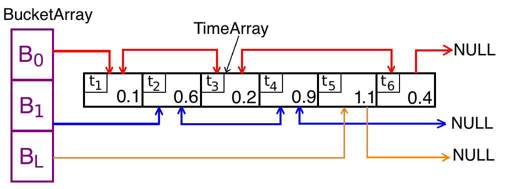
Figure 1. TimeArray and BucketArray for $M=6$, $Q=2$ and $\tau=1$. The TimeArray stores times of occurrence of all $6$ clocks, labeled $t_{1}$ to $t_{6}$. Three buckets stored in the BucketArray, labeled $B_{0}$, $B_{1}$, and $B_{L}$, contain times of occurrence between $0$ and $0.5$, between $0.5$ and $1.0$, and greater than $1.0$, respectively. Arrows represent the direction of pointers

The HLM can be summarized as follows

1. Initialization:

   • Initialize $R_{i}$s. Initialize $X_{0}$. Let $t=0$.

   • Generate the dependency graph $G$.

   • Generate times of occurrence $t_{1},\cdots,t_{M}$.

   • Initialize TimeArray, RateArray, and BucketArray

2. Choose proper parameters $\tau$ and $Q$.

3. Distribute times of occurrence to corresponding buckets BucketArray[0] $\sim$ BucketArray[Q].

4. For $i=0$ to $Q-1$

   While BucketArray[i] is nonempty:

   • Find the least time of occurrence $t_{l}$ within this bucket

   • Make update according to $T_{l}$

   • Follow the dependency graph $G$ to update all affected rate functions in RateArray

   • Update time of occurrence of all affected events as (3.1) and move affected elements in TimeArray to the corresponding buckets.

   • Advance $t_{l}$ by an exponential random number with rate $R_{l}$ and move TimeArray[l] to the corresponding bucket

5. Update the time intervals of each bucket and return to 3, or quit.

4.2. Analysis of algorithm

It is important to demonstrate the correctness of the HLM before further investigations. In fact, the HLM is mathematically equivalent to the NRM. This can be checked by using the following three steps.

1. Sampling events Sampling the next time of occurrence is the core step of the SSA. In the HLM, the next time of occurrence is chosen as the minimum of $M$ random times, which is equivalent to the NRM and the FRM.

2. Reusing random times. After initialization, a sample of the time of occurrence of each clock is taken from the corresponding exponential distribution. If an event occurs at time $t$ without changing the rate of this clock, this sample can be reused due to the time-invariant nature of the exponential distribution. More precisely, if $Z$ is an exponentially distributed random variable, then for any $t>0$, the “overshoot”, i.e., $Z|_{Z>t}$, has the same exponential distribution. We refer Theorem 1 in [16] for the full mathematical detail.

3. Changing clock rates. The update transformation in an event may change the rate of other clocks. Therefore the affected times of occurrence need to be updated accordingly.

   Assume after an event at time $t$, the rate of the $i$-th clock changes from $R^{old}_{i}$ to $R^{new}_{i}$. By step 2, the “overshoot” $t_{i}-t$ has an exponential distribution with rate $R^{old}_{i}$. In addition, it is a simple probabilistic fact that for any constant $a>0$ and any exponential random variable $Z$ with rate $r$, $aZ$ is exponentially distributed with rate $r/a$. Hence the transformation in equation (3.1) maps an exponential distribution with rate $R^{old}_{i}$ to an exponential distribution with rate $R^{new}_{i}$. For further reference regarding the proof, see Theorem 2 in [16].

4.3. Analysis of complexity

1. Average computational cost.

   Assume

   • There exists a constant $K$ independent of $M$ such that

     $$\mathbb{E}[\mbox{Number of events occurring on }[t\,,t+\Delta]]\leq KM\Delta$$

     for any $t$ and any $\Delta>0$; and

   • The dependence graph is sparse such that the maximum out degree is $O(1)$.

   Then if $\tau\sim O(1)$, $O(M)$ events occur in each time step with length $\tau$. The computational cost of a bucket redistribution is $M$. If we choose $Q\sim O(M)$, then the number of events in each bucket can be (very) roughly approximated by a Poisson distribution with $O(1)$ mean. Since the dependency graph is sparse, the average cost of updating each bucket is $O(1)$. Therefore the total computational cost in one step is $O(M)+Q\times O(1)=O(M)$. This makes the average complexity of the HLM be $O(1)$ per event.

   If the dependency graph is not sparse in a way that the average out degree of vertices is $D$, which is possibly dependent of $M$, then the average cost of updating each bucket is $O(D)$. This brings the total computational cost in one step to $O(DM)$ and the average complexity per event to $O(D)$.

   We remark that assumptions (a) and (b) are satisfied by a large class of models in practice. In particular, if $R_{max}\sim O(1)$ and $R_{max}/R_{min}\sim O(1)$, then (a) is satisfied.

2. Worst case analysis. In the worst case, which means all events are distributed into the same bucket, the HLM is equivalent to the FRM. Therefore, the computational cost per event in the worst case is $O(M)$. However, we remark that in most practical cases, this worst situation occurs with an extremely low probability. If $R_{max}\sim O(1)$ and $R_{max}/R_{min}\sim O(1)$, when letting $Q\sim O(M)$ and $\tau\sim O(1)$, the probability that all $M$ events are placed into a single bucket is $\sim O(M^{-M})$.

4.4. Discussion of issues

1. Choice of parameters.

   Finding optimal parameters for the HLM is a challenging job. We make some idealized calculations to shed some light on this problem. Assume (a) and (b) in Section 4.3 hold. Then the average computational cost per event, denoted by $\mathcal{C}$, on this time step satisfies

   $$\mathcal{C} = \frac{1}{\#events}\bigg{\{}search\,\,cost+update\,\,cost$$

   $$+bucket\,\,iteration\,\,cost+bucket\,\,redistribution\,\,cost\bigg{\}}$$

   $$= \frac{O(1)}{\alpha M\tau}\bigg{\{}C_{s}Q\cdot\frac{1}{2}\left[(\frac{\alpha M\tau}{Q})^{2}+2\frac{\alpha M\tau}{Q}\right]+C_{u}\alpha M\tau$$

   $$+C_{i}Q+C_{r}M\bigg{\}}\,,$$

   where $C_{s}$, $C_{u}$, $C_{i}$, and $C_{r}$ represent the average cost of searching, updating events, bucket iteration, and bucket redistribution. Therefore, it is easy to check that for each fixed $\tau$, the optimal $Q$ satisfies

   $$Q_{opt}=\alpha M\tau\cdot\sqrt{\frac{C_{s}}{2C_{i}}}\,.$$

   When $Q$ is optimal, we have

   $$\mathcal{C}=\sqrt{2C_{s}C_{i}}+C_{s}+C_{u}+\frac{C_{r}}{\alpha\tau}\,.$$

   It is reasonable to assume $C_{s}$, $C_{i}$, and $C_{r}$ are constants. But $C_{u}$ depends on $\tau$ because we do not relink pointers if an update does not move the affected event to a new bucket. For smaller $\tau$, larger proportion of events will remain in the bucket $B_{L}$ throughout the step. Hence a more precise model of $C_{u}$ is

   $$C_{u}=C_{u}(\tau)=C^{\prime}_{u}+C^{\prime\prime}_{u}(1-e^{-\alpha\tau})\,,$$

   where $C^{\prime}_{u}$ and $C^{\prime\prime}_{u}$ are constants that represent the cost of update without relinking pointers and the cost of relinking pointers.

   Therefore, we conclude that the optimal number of buckets $Q$ is in proportion to both $\tau$ and $M$, and the optimal value of $\tau$ depends on constants $C^{\prime\prime}_{u}$, $C_{r}$, and $\alpha$.

   One important remark is that the empirical performance of the HLM is not sensitive with respect to small change of parameters. The reason is that updating an event, which includes calculating new rate functions, modifying times of occurrence, and relinking pointers, is much more expensive than the other operations. Hence $C_{u}$ is significantly greater than the other three constants. Similarly, $C^{\prime}_{u}$ is greater than $C^{\prime\prime}_{u}$. According to our test, the performance of the HLM is stable as long as $Q\sim O(M)$ and $\tau\sim O(1)$. For example, for the generalized KMP model introduced in Section 5.1, the CPU time with $\tau=1,Q=M$ and that with $\tau=1,Q=M/10$ have only less than $10\%$ difference.

   When simulating models in Section 5, we choose smaller $\tau$ such that about half of events are placed into $B_{L}$, then make $Q$ be in proportion to $\tau$ and $M$. We admit that these parameters may not be optimal. To obtain the optimal parameters, all constants introduced above should be estimated empirically. In other words, the algorithm needs to be enhanced such that $\tau$ and $Q$ can be properly adjusted as the simulation proceeds. We will make this extension in our subsequent works.

2. Possible improvements.

   There are two places to further improve the HLM. The first potential improvement is at the level of implementation. One can replace the linear search in each bucket with a binary search. Under our assumption, the expectation of the largest number of events stored in a bucket is $O(\log M)$. Therefore, a binary search could potentially increase the performance of the algorithm. As mentioned before, it is slightly less efficient to implement buckets as linear arrays than to implement them as linked lists. However, we expect some improvement if buckets are implemented as linear arrays, with binary heaps constructed on them. ( It is standard knowledge that implementing a binary heap as a linked list is significantly more complicated than implementing that as a linear array. ) We did not present this improvement in the present paper because it does not change the $O(1)$ computational complexity per event of the HLM. Plus due to the overhead of constructing the binary heap, we expect the improvement can only be observed for very large scale problems.

   The second improvement is for Markov jump processes with sparse dependency graphs. Assuming $R_{max}/R_{min}\sim O(1)$, when the dependency graph is sparse, times of occurrence stored in each bucket will not affect each other with high probability ($\sim 1-O(1/M)$). Therefore, in most situations we can update times of occurrence in each bucket sequentially from the head of the list without searching for the minimum. Since in average a bucket only contains $O(1)$ events, this improvement does not change the computational complexity of the algorithm either. In fact, we only observed a minor increase of simulation speed at the cost of much more complicated programming code. However, this idea can be used in the parallelization of our algorithm, as explained in (3).

3. Parallelization.

   Although the fact that events in one bucket are “almost independent” does not significantly improve the performance of the HLM when running on a single CPU, it can be used to parallelize this algorithm. In fact, the HLM is very compatible with parallel programming if the dependency graph is sparse. The idea is to make the number of buckets $Q\sim O(M/p)$, where $p$ is the number of CPUs, and divide one bucket into $p$ sub-buckets. During the bucket redistribution, we can evenly distribute events into sub-buckets that are maintained by different CPUs. Suppose the dependency graph is sparse, then events placed in each bucket will not affect each other with high probability. Therefore in most of the running time, different CPUs can update events in their own sub-buckets independently.

   The principle of the parallelization is straightforward. However, there are lots of details remaining to be studied. With a low but strictly positive probability, an event in one bucket can affect events in the same bucket (but probably different sub-bucket), which will cause intensive communication between CPUs. Therefore, it is crucial to design algorithms that can identify and deal with these small probability events with the lowest overall overhead. We will study the parallel HLM and its applications intensively in our subsequent works.

5. Numerical Examples

5.1. Introduction to models

We chose the following four models to test the performance of the HLM.

(i). Generalized KMP model. There are numerous stochastic processes in the field of statistical mechanics that fit the generic description of $X_{t}$ in Section 2, such as the simple inclusion process (SIP), the simple exclusion process (SEP) and its variants [3, 12, 11], and many stochastic processes that models the microscopic heat conduction [13, 24, 4]. We chose the following generalized KMP model as a test case of our simulation. The KMP model is a stochastic model proposed in [21] that models the microscopic energy transport, from which a microscopic derivation of Fourier’s law was carried out. The main feature of the generalized KMP model ( See [23, 20] for details ) here is its energy dependent clock rates, which makes the simulation non-trivial.

The KMP model models the energy transport in a 1D chain of $M$ oscillators coupled with two heat baths whose temperatures are $\mathcal{T}_{L}$ and $\mathcal{T}_{R}$, respectively. We only take note of energy carried by each oscillator, denoted by $x_{1},\cdots,x_{M}$, respectively. The Markov chain generated by the KMP model can be described as follows. An exponential clock with rate $R(x_{i},x_{i+1}),i=0\sim M$ is associated with each pair of adjacent oscillators (let $x_{0}=\mathcal{T}_{L}$ and $x_{M+1}=\mathcal{T}_{R}$). When the clock rings, the energy stored in the corresponding pair of oscillators is pooled together, repartitioned randomly, and redistributed back to the oscillators. The energy redistribution satisfies

$$(x_{i}^{\prime},x^{\prime}_{i+1})=\left(p(x_{i}+x_{i+1}),(1-p)(x_{i}+x_{i+1})\right)\,,$$

where $p$ is a uniform random variable on $(0,1)$ that is independent of everything else, and $x_{i}^{\prime}$ is the energy carried by oscillator $i$ after the update. If clock $0$ (resp. clock $M$) rings, the energy of the first (resp. last) oscillator exchanges energy with an exponential random variable with mean $\mathcal{T}_{L}$ (resp. $\mathcal{T}_{R}$) in the same way.

We let $\mathcal{T}_{L}=1.0$, $\mathcal{T}_{R}=2.0$, and $R(x_{i},x_{i+1})=\sqrt{x_{i}+x_{i+1}}$ and simulate the generalized KMP model with varying $M$s.

Markov jump processes arising in other statistical mechanics models may not satisfy the generic description of $X_{t}$ in Section 2. However, they can still be simulated by the HLM efficiently. One example is the random halves model proposed in [13] and its modification in [24], in which the number of clocks varies randomly with time instead of being a constant. When the number of exponential clocks changes by one, the cost of maintaining the bucket data structure is $O(1)$. In contrast, in the NRM, the computational cost of maintaining the binary heap after adding/removing one exponential clock is $O(\log M)$.

(ii). Chemical reaction network The second example we chose is a chemical reaction network. Stochastic chemical reaction networks are a very important class of Markov jump process. It is well known that most SSA methods were originally developed for the stochastic simulation of chemical reactions. To simplify the implementation, we use the same example in [28] with minor modification.

Consider a large chemical reaction network with $M$ reactions. For the sake of simplicity we only take note of rate functions, or the propensity. The initial propensities are uniformly distributed over $[0,\,2]$. The dependency graph is randomly generated in a way that each reaction affects $m$ other reactions, where $m$ is a random integer uniformly distributed over $\{1,\cdots,30\}$. After the occurrence of each reaction, all affected reactions are updated in a way that the propensity is replaced by a new random number uniformly distributed on $[0,\,2]$. We note that this example is different from real-world chemical reaction networks, and is used only for the purpose of testing algorithms.

The main difference between our example and the example presented in [28] is that we do not bound the ratio of $R_{max}$ to $R_{min}$. In the example used by [28], the ratio of $R_{max}$ to $R_{min}$ is bounded by $1\times 10^{6}$ at the initial state and has minor changes when the simulation proceeds.

(iii). Reaction-diffusion system The third example we chose is the Gray-Scott model, which is a reaction-diffusion system in 2D. Since the purpose of this simulation is to compare the performance of algorithms, we simplify some details. The Gray-Scott model is well known as its pattern formation phenomenon [29], as seen in Fig 2. The reaction part of the model involves two species $U$ and $V$ and four reactions

$$U+2V \xrightarrow{K_{1}(\Omega)} 3V$$

$$U \xrightarrow{K_{f}} \emptyset$$

$$V \xrightarrow{K_{2}} \emptyset$$

$$\emptyset \xrightarrow{K_{f}u_{0}(\Omega)} U$$

where $\Omega$ is a parameter that indicates the scale of the system per subvolume. $\Omega$ is determined by both the molecular population level and the edge length of subvolumes, which are assumed to be constants throughout this example. Parameters $k_{1}(\Omega)=\hat{k}_{1}\Omega^{-2}$ and $u_{0}(\Omega)=\hat{u}_{0}\Omega$ depend on $\Omega$. $\hat{k}_{1},K_{f},K_{2},\hat{u}_{0}$ are constants. Molecules are assumed to be well-mixed in each subvolume. Besides reactions, $U$ and $V$ molecules can jump to neighbor subvolumes at certain diffusion rates, denoted by constants $D_{U}$ and $D_{V}$, respectively. $D_{U}$ and $D_{V}$ also depend on the edge length of subvolumes.

In the simulation, we study domains that are consist of $K\times K$ subvolumes for $K$ ranging from $3$ to $1200$. Numbers of molecules of species $U$ and $V$ in each subvolume are denoted by $U_{i,j}$ and $V_{i,j}$, respectively, where $i,j$ ranges from $1$ to $K$. There are six exponential clocks associated with each subvolume with rates $U_{i,j}V_{i,j}^{2}K_{1}(\Omega)$, $U_{i,j}K_{f}$, $V_{i,j}K_{f}$, $K_{f}u_{0}(\Omega)$, $U_{i,j}D_{U}$, and $V_{i,j}D_{V}$, respectively. When the diffusion clock rings, one corresponding molecule in the subvolume moves to one of its nearest neighbors with equal probability. A molecule exits from the system if it moves out of the domain. Hence the scale of this system is $M=6K^{2}$. The values of parameters are taken as $\Omega=250$, $K_{f}=0.0055$, $K_{2}=0.0205$, $D_{V}=0.002$, $D_{U}=0.001$, and $\hat{k}_{1}=\hat{u}_{0}=1$.

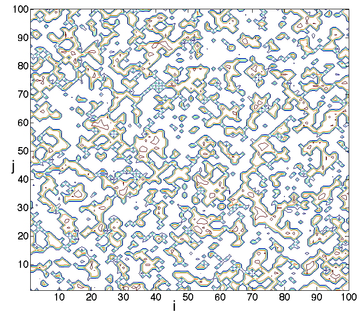
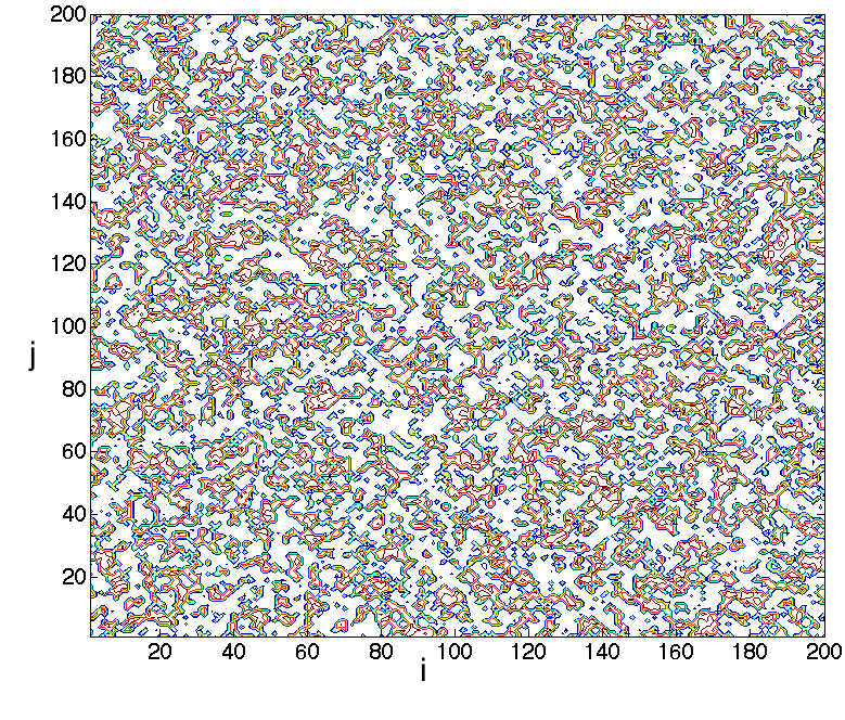
Figure 2. Pattern formation of the Gray-Scott model. Figure 2 (a): Contour plots of numbers of $U$ molecules on $100\times 100$ subvolumes at $t=1500.0$. Figure 2(b): Contour plots of numbers of $U$ molecules on $200\times 200$ subvolumes at $t=1500.0$

(iv). Chemical oscillator system.

To examine the performance of the HLM for small scale problems, we consider the following chemical oscillator system called the “Oregonator”, which was originally introduced in [15]. The “Oregonator” is a chemical reaction system with five reactions

$$\bar{X}_{1}+Y_{2} \xrightarrow{c_{1}} Y_{1}$$

$$Y_{1}+Y_{2} \xrightarrow{c_{2}} Z_{1}$$

$$\bar{X}_{2}+Y_{1} \xrightarrow{c_{3}} 2Y_{1}+Y_{3}$$

$$2Y_{1} \xrightarrow{c_{4}} Z_{2}$$

$$\bar{X}_{3}+Y_{3} \xrightarrow{c_{5}} Y_{2}\,,$$

where the molecular population level of species $\bar{X}_{1},\bar{X}_{2}$, and $\bar{X}_{3}$ are assumed to be constants. The parameters are taken to be $c_{1}\bar{X}_{1}=2$, $c_{2}=0.1$, $c_{3}\bar{X}_{2}=104$, $c_{4}=0.016$, and $c_{2}\bar{X}_{3}=26$, which are consistent with [18].

5.2. Performance test of HLM

(i). Speed of simulation

The first set of numerical simulations concern the speed of algorithm. We implement each of the four models introduced in the previous subsection using four different methods: the CRM, the DM, the HLM, and the NRM. All SSA methods are implemented in C, with C++ I/O for the sake of simplicity of coding. Implementations of all algorithms are optimized to the best of our ability. For example, in the implementation of the CRM, instead of dynamic group bounds varying with $R_{min}$, pre-assigned group bounds are used to reduce the overhead of maintaining groups. All performance tests are run on a 2012 Macbook Pro laptop with an Intel Core I7-3615QM CPU and $8$ GB memory.

Instead of stopping after simulating a fixed number of events, we chose to simulate all examples up to $t=10$, as simulating Markov processes up to different times may bias the result. The performance of four SSA methods is measured in seconds per million events and compared. The scales of the generalized KMP model, the chemical reaction network, and the reaction-diffusion system ranges from $M=10\sim 10^{7}$, $M=50\sim 5\times 10^{6}$, and $M=54\sim 8.64\times 10^{6}$, respectively.

The parameters of the HLM are chosen as $\tau=0.2$, $Q=M/10$ for the generalized KMP model, $\tau=0.1$, $Q=M/20$ for the chemical reaction network, $\tau=0.5$, $Q=M/2$ for the reaction-diffusion system, and $\tau=0.01$, $Q=5$ for the “Oregonator”. The parameter of the CRM is chosen as $g=30$ for all models.

In examples 5.1 (i) – (iii) , CPU times ( seconds per million events) vs. $M$ of all four SSA methods are plotted in linear-log plots and presented in Figure 3, 4, and 5. In these figures, each plot represents the mean CPU times of $10$ runs. The error bars indicate one standard deviation of the mean. The CPU times ( seconds per million events) of four SSA methods over $10$ runs of the “Oregonator” are presented in Figure 6. The error bars also represent one standard deviation.

As shown in these figures, for large scale models, the HLM is superior to the other SSA methods in all tested examples. Although having the same computational complexity, we find that the HLM is slightly faster than the CRM in all examples and all system sizes. One possible reason is that maintaining groups in the CRM is more expensive than maintaining buckets in the HLM. The CRM also generates more random numbers than the HLM. For small scale models, we find that the performance of the HLM is slower than the DM (and sometimes the NRM) but remains competitive.

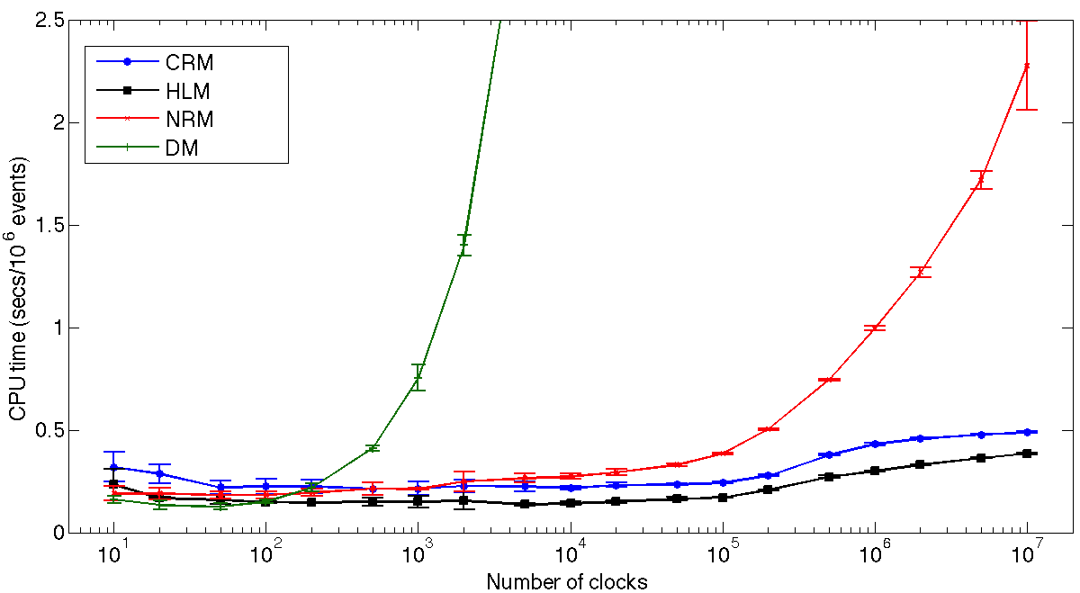
Figure 3. CPU times in seconds per $10^{6}$ events vs. number of exponential clocks for the generalized KMP model. Blue, black, red, and green plots represent the mean CPU times of the CRM, the HLM, the NRM, and the DM over $10$ runs, respectively. The error bars indicate one standard deviation of the mean.

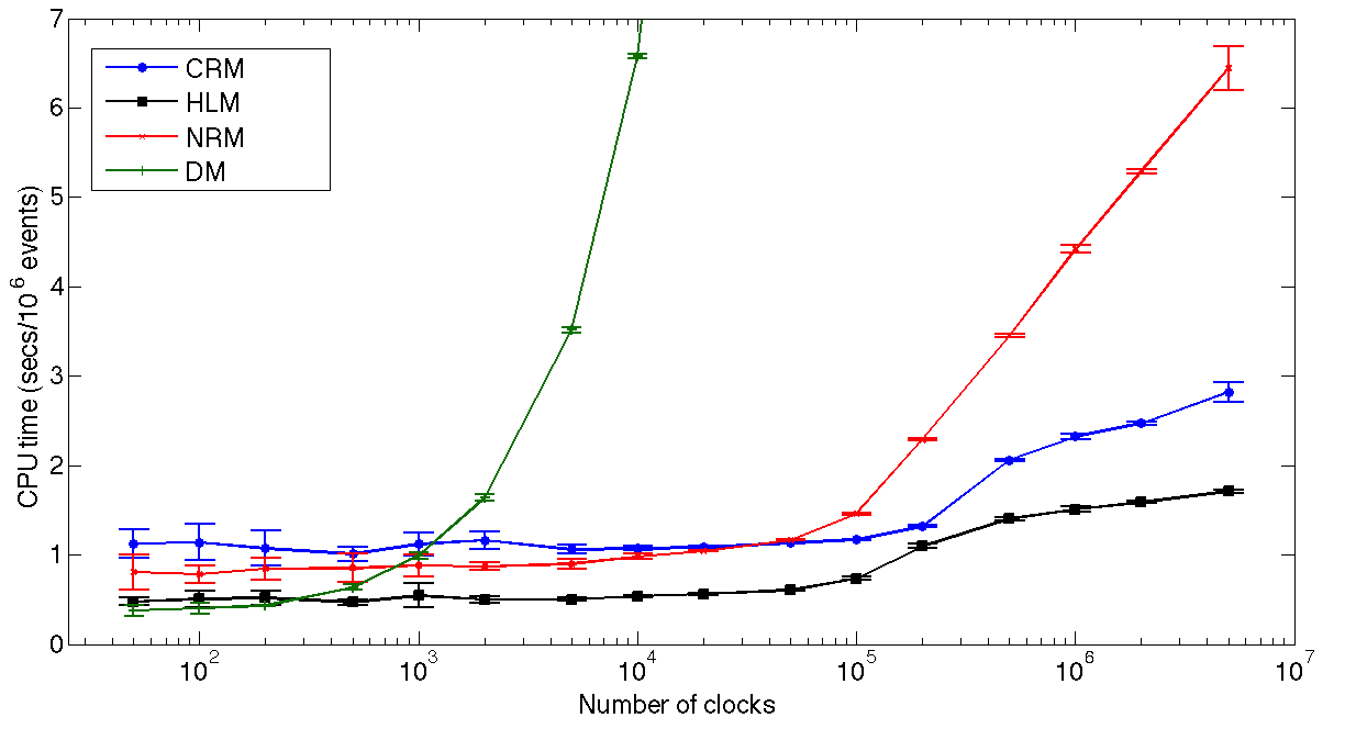
Figure 4. CPU time in seconds per $10^{6}$ events vs. number of exponential clocks for the chemical reaction network. Blue, black, red, and green plots represent the mean CPU times of the CRM, the HLM, the NRM, and the DM over $10$ runs, respectively. The error bars indicate one standard deviation of the mean.

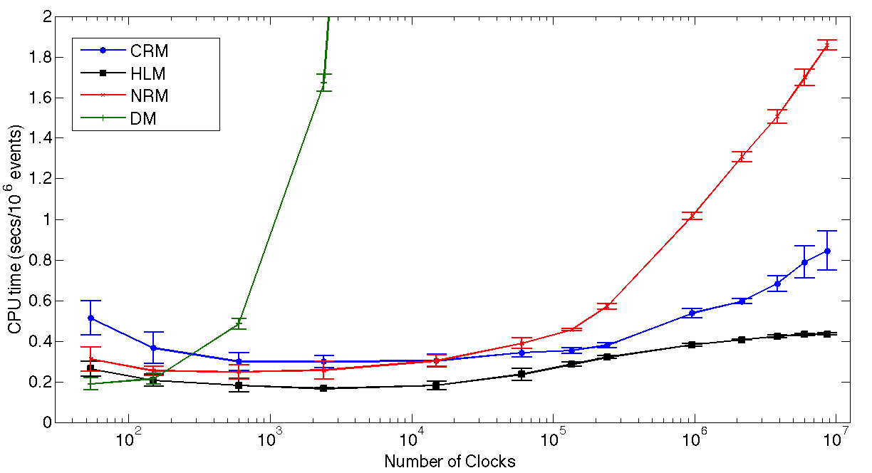
Figure 5. CPU time in seconds per $10^{6}$ events vs. number of exponential clocks for the reaction-diffusion model. Blue, black, red, and green plots represent the mean CPU times of the CRM, the HLM, the NRM, and the DM over $10$ runs, respectively. The error bars indicate one standard deviation of the mean.

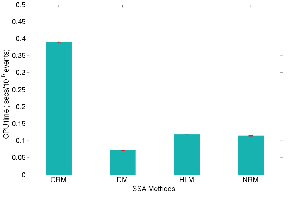
Figure 6. CPU time in seconds per $10^{6}$ events vs. number of exponential clocks for the “Oregonator” model. Heights of bars represent the mean CPU times of the CRM, the HLM, the NRM, and the DM over $10$ runs, respectively. The red error bars indicate one standard deviation of the mean.

(ii). Statistics of computer operations

The running time of an algorithm depends on many things beyond the efficiency of algorithms. Details of implementation, the compiler, the operating system, and the size of CPU cache can significantly change the empirical CPU times. Therefore, it is important to study the average number of operations per event of the HLM.

We collect data of computer operations of examples 5.1 (i) – (iii) . The number of comparisons when linearly searching a bucket and the number of moves of events between buckets are recorded. Our results confirm that, in all three examples, the HLM has constant computational cost per event. The total numbers of comparisons plus moves per event are $\approx 5.0$ for the generalized KMP model, $\approx 10.5$ for the reaction diffusion system, and $\approx 27.5$ for the chemical reaction network, respectively. As an example of $O(1)$ algorithm vs. $O(\log M)$ algorithm, the statistics of computer operations of the HLM vs. the NRM for the generalized KMP model are demonstrated in Figure 7, in which the number of moves of events are further broken down into moves with relinking pointers and moves without relinking pointers (i.e. within the same bucket). The number of operations of the NRM shown in the figure is the number of swaps in the binary heap. We find that the HLM is more efficient than the NRM when $M$ is greater than $10^{2}$.

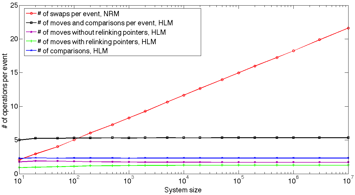
Figure 7. Number of operations per event of the generalized KMP model. Red: number of swaps per event of the NRM. Black: number of moves and comparisons per event of the HLM. Purple: number of moves (without relinking pointers) per event of the HLM. Green: number of moves (with relinking pointers) per event of the HLM. Blue: number of comparisons per event of the HLM. Parameters are same as in Section 5.2 (i).

6. Conclusion

In the present paper, we introduced a fast method for the stochastic simulation algorithm (SSA), namely the Hashing-Leaping Method (HLM), for a class of Markov jump processes arising in many scientific fields. The common feature of these Markov jump processes is that they are driven by many heterogeneous, state-dependent exponential clocks. The number of exponential clocks, or the scale of the system, is denoted by $M$. As the Markov jump process proceeds at a sequence of random times, the main strategy of the SSA is to identify the next time of occurrence among many exponential random times. To do so, the HLM uses a hash-table-like data structure to distribute times of occurrence covered by a certain time step with length $\tau$ into $Q$ evenly divided buckets, updates all buckets sequentially, and leaps forward by $\tau$. Under assumptions (a) and (b) in Section 4.3, the average computational cost per event of the HLM is $O(1)$, independent of the number of exponential clocks.

For large scale Markov jump processes, the HLM has the desired performance. The speed of the HLM is tested with three large-scale models: a generalized KMP model, a chemical reaction network, and a stochastic reaction-diffusion system. Our simulation results showed advantages of the HLM over the DM, the NRM, and the CRM when $M$ is greater than $\sim 10^{2}$. In addition, we verified numerically that the average number of computer operations per event of the HLM is $O(1)$.

It is well accepted that no SSA method is unconditionally superior to the rest. For small-scale problems, Gillespie’s direct method (DM) usually has the best efficiency. This is confirmed by our simulation result of a chemical oscillator model called the “Oregonator”. For this small-scale model (in which $M=5$), the performance of the HLM remains competitive. While possibly due to the overhead of maintaining many groups, as the only other existing conditional $O(1)$ per-event SSA method to the best of our knowledge, the CRM is slower than the rest SSA methods when the scale of the Markov process is sufficiently small.

We do not claim that the HLM is a perfect algorithm. One drawback is that the performance of the HLM depends on the choice of parameters. According to our analysis in Section 4.4, the optimal parameters depend on some constants that should be estimated empirically. Although the performance of the HLM is not sensitive with respect to change of parameters as long as $\tau\sim O(1)$ and $Q\sim O(M)$, to reach the full efficiency of the HLM, some empirical estimations or small scale CPU time tests are be needed at the current stage. To partially solve this problem, in future, we will develop algorithms that can adjust parameters as the simulation proceeds.

Overall, our analysis and numerical simulations show that the HLM is a promising SSA method, especially for large scale Markov processes. The performance of the HLM can be potentially improved in several aspects, from more efficient implementations to parallelizations. It is also useful to trim the HLM for specific problems, such as multiple time scale systems and systems with varying number of exponential clocks. Those issues will be studied in our subsequent works.

References

- [1] Farid F Abraham and George M White, Computer simulation of vapor deposition on two-dimensional lattices, Journal of Applied Physics 41 (1970), no. 4, 1841–1849.
- [2] JR Beeler Jr, Displacement spikes in cubic metals. i. -iron, copper, and tungsten, Physical Review 150 (1966), no. 2, 470.
- [3] C Boldrighini, G Cosimi, S Frigio, and M Grasso Nunes, Computer simulation of shock waves in the completely asymmetric simple exclusion process, Journal of Statistical Physics 55 (1989), no. 3-4, 611–623.
- [4] Federico Bonetto, Joel L Lebowitz, and Luc Rey-Bellet, Fourier’s law: A challenge for theorists, arXiv preprint math-ph/0002052 (2000).
- [5] Alfred B Bortz, Malvin H Kalos, and Joel L Lebowitz, A new algorithm for monte carlo simulation of ising spin systems, Journal of Computational Physics 17 (1975), no. 1, 10–18.
- [6] Yang Cao, Dan Gillespie, and Linda Petzold, Multiscale stochastic simulation algorithm with stochastic partial equilibrium assumption for chemically reacting systems, Journal of Computational Physics 206 (2005), no. 2, 395–411.
- [7] Yang Cao, Daniel T Gillespie, and Linda R Petzold, Efficient step size selection for the tau-leaping simulation method, The Journal of chemical physics 124 (2006), no. 4, 044109.
- [8] Yang Cao, Hong Li, and Linda Petzold, Efficient formulation of the stochastic simulation algorithm for chemically reacting systems, The journal of chemical physics 121 (2004), no. 9, 4059–4067.
- [9] Yang Cao and Linda Petzold, Slow-scale tau-leaping method, Computer methods in applied mechanics and engineering 197 (2008), no. 43, 3472–3479.
- [10] Vincent Danos, Jérôme Feret, Walter Fontana, and Jean Krivine, Scalable simulation of cellular signaling networks, Programming Languages and Systems, Springer, 2007, pp. 139–157.
- [11] Bernard Derrida, An exactly soluble non-equilibrium system: the asymmetric simple exclusion process, Physics Reports 301 (1998), no. 1, 65–83.
- [12] Bernard Derrida, Steven A Janowsky, Joel L Lebowitz, and Eugene R Speer, Exact solution of the totally asymmetric simple exclusion process: shock profiles, Journal of statistical physics 73 (1993), no. 5-6, 813–842.
- [13] J-P Eckmann and L-S Young, Nonequilibrium energy profiles for a class of 1-d models, Communications in Mathematical Physics 262 (2006), no. 1, 237–267.
- [14] Johan Elf and Måns Ehrenberg, Spontaneous separation of bi-stable biochemical systems into spatial domains of opposite phases, Systems biology 1 (2004), no. 2, 230–236.
- [15] Richard J Field and Richard M Noyes, Oscillations in chemical systems. iv. limit cycle behavior in a model of a real chemical reaction, The Journal of Chemical Physics 60 (1974), no. 5, 1877–1884.
- [16] Michael A Gibson and Jehoshua Bruck, Efficient exact stochastic simulation of chemical systems with many species and many channels, The journal of physical chemistry A 104 (2000), no. 9, 1876–1889.
- [17] Daniel T Gillespie, A general method for numerically simulating the stochastic time evolution of coupled chemical reactions, Journal of computational physics 22 (1976), no. 4, 403–434.
- [18] by same author, Exact stochastic simulation of coupled chemical reactions, The journal of physical chemistry 81 (1977), no. 25, 2340–2361.
- [19] by same author, Approximate accelerated stochastic simulation of chemically reacting systems, The Journal of Chemical Physics 115 (2001), no. 4, 1716–1733.
- [20] Alexander Grigo, Konstantin Khanin, and Domokos Szasz, Mixing rates of particle systems with energy exchange, Nonlinearity 25 (2012), no. 8, 2349.
- [21] C Kipnis, C Marchioro, and E Presutti, Heat flow in an exactly solvable model, Journal of Statistical Physics 27 (1982), no. 1, 65–74.
- [22] M Kotrla, Numerical simulations in the theory of crystal growth, Computer Physics Communications 97 (1996), no. 1, 82–100.
- [23] Yao Li and Lai-Sang Young, Existence of nonequilibrium steady state for a simple model of heat conduction, Journal of Statistical Physics 152 (2013), no. 6, 1170–1193.
- [24] by same author, Nonequilibrium steady states for a class of particle systems, Nonlinearity 27 (2014), no. 3, 607.
- [25] Carl Adam Petri, Kommunikation mit automaten, Ph.D. thesis, University of Bonn, 1962.
- [26] Rajesh Ramaswamy, Nélido González-Segredo, and Ivo F Sbalzarini, A new class of highly efficient exact stochastic simulation algorithms for chemical reaction networks, The Journal of chemical physics 130 (2009), no. 24, 244104.
- [27] Rajesh Ramaswamy and Ivo F Sbalzarini, A partial-propensity variant of the composition-rejection stochastic simulation algorithm for chemical reaction networks, The Journal of chemical physics 132 (2010), no. 4, 044102.
- [28] Alexander Slepoy, Aidan P Thompson, and Steven J Plimpton, A constant-time kinetic monte carlo algorithm for simulation of large biochemical reaction networks, The journal of chemical physics 128 (2008), no. 20, 205101.
- [29] Matthias Vigelius and Bernd Meyer, Stochastic simulations of pattern formation in excitable media, PloS one 7 (2012), no. 8, e42508.
- [30] Arthur F Voter, Introduction to the kinetic monte carlo method, Radiation Effects in Solids, Springer, 2007, pp. 1–23.
- [31] E Weinan, Di Liu, and Eric Vanden-Eijnden, Nested stochastic simulation algorithm for chemical kinetic systems with disparate rates, The Journal of chemical physics 123 (2005), no. 19, 194107.
- [32] Jin Yang, Michael I Monine, James R Faeder, and William S Hlavacek, Kinetic monte carlo method for rule-based modeling of biochemical networks, Physical Review E 78 (2008), no. 3, 031910.