Power Systems Without Fuel

Abstract

The finiteness of fossil fuels implies that future electric power systems may predominantly source energy from fuel-free renewable resources like wind and solar. Evidently, these power systems without fuel will be environmentally benign, sustainable, and subject to milder failure scenarios. Many of these advantages were projected decades ago with the definition of the soft energy path, which describes a future where all energy is provided by numerous small, simple, and diverse renewable sources. Here we provide a thorough investigation of power systems without fuel from technical and economic standpoints. The paper is organized by timescale and covers issues like the irrelevance of unit commitment in networks without large, fuel-based generators, the dubiousness of nodal pricing without fuel costs, and the need for new system-level models and control methods for semiconductor-based energy-conversion interfaces.

I Introduction

Eventually, whether from a deliberate shift to renewables or the depletion of planetary fossil fuel sources, major portions of power systems will run without fossil fuels. There is now extensive literature on this subject, see, e.g., [1, 2], most of which focuses on the advantages and disadvantages of renewable energy sources. Here we also consider this scenario, but focus on the combined consequences of using renewables and eliminating fuel-based generators; we fully define our scope in Section I-B. We believe that it is important to discuss these issues both for the limiting case of exclusively renewable power production and also under mostly renewable power production, in which case planning and operational practices should reflect the large majority of renewables instead of a small minority of fuel-based generators.

Much of the salient physics of present-day power systems are attributable to fuel-based generators, which are most cost-effective at large unit sizes; for example, thermal limits constrain power production schedules, and synchronous machine rotor inertias dominate transient stability. While the addition of intermittent and distributed renewables will change the form of power systems, so will removing the fuel-based generators that account for much of its current character. Many of the consequences of removing fuel-based generators are well studied, for example the loss of system inertia and the need to replace generator reserves with storage and demand response. However, it is our perception that many important issues have not been thoroughly discussed, such as the need for new optimal power flow objectives to replace fuel costs and the attendant need for alternative economic mechanisms to nodal pricing. In some cases, removing fuel-based generators can result in significant benefits like the elimination of the unit commitment problem and the viability of transitioning to a predominantly DC infrastructure. We address such issues in a unified fashion by surveying existing discussions, identifying challenges, and suggesting new directions where appropriate.

Two key motifs of this paper are that (see Fig. 1)

• all timescales are shrinking, and

• a few large components will be replaced by numerous small components.

These changes have a number of salient consequences. For instance, renewables can be installed and maintained more quickly than fuel-based generators, bulk generation need not be scheduled days in advance to accommodate stringent startup and shutdown constraints, and the loss of mechanical inertia implies that transients will be dominated by the dynamic behaviors of many small, fast power-electronic energy-conversion interfaces. We partially structure our discussions around timescales by first considering long-term planning, then steady-state operation, and then transient dynamics. While so doing, we additionally highlight the emergence and disappearance of new and old couplings. For example, renewable intermittency couples hourly steady-state dispatch decisions to regulation requirements. Similarly, wind and solar power sources consume negligible quantities of water compared to the cooling needs of fuel-based generators, drastically reducing the power system’s dependency on the water infrastructure.

I-A The soft energy path and the status quo

The rationale for a fully renewable energy infrastructure has long been well established; we now briefly summarize its beginnings and provide a few modern examples. In 1976, Lovins described the soft energy path as a future in which societal energy needs are met by numerous small, simple, diverse technologies that rely on renewable energy sources [3, 4]. The soft energy path stands in contrast to the hard energy path, wherein energy is provided by a few large, resource intensive, complex technologies which inevitably induce caustic political dependencies and are prone to expensive physical failures. The case for the soft energy path—which we note, does not include nuclear power—has been restated and reaffirmed in many ways over the past four decades; for instance, the capability of wind and solar to fulfill all of our energy needs is addressed in [5]. Distributed generation [6] and microgrids [7] are two related architectural paradigms where small, renewable technologies meet energy needs locally. Another compelling argument for the soft energy path is that unused wind and solar energy are lost while fossil fuels may be indefinitely “… [left] … in the ground for emergency use only” [3].

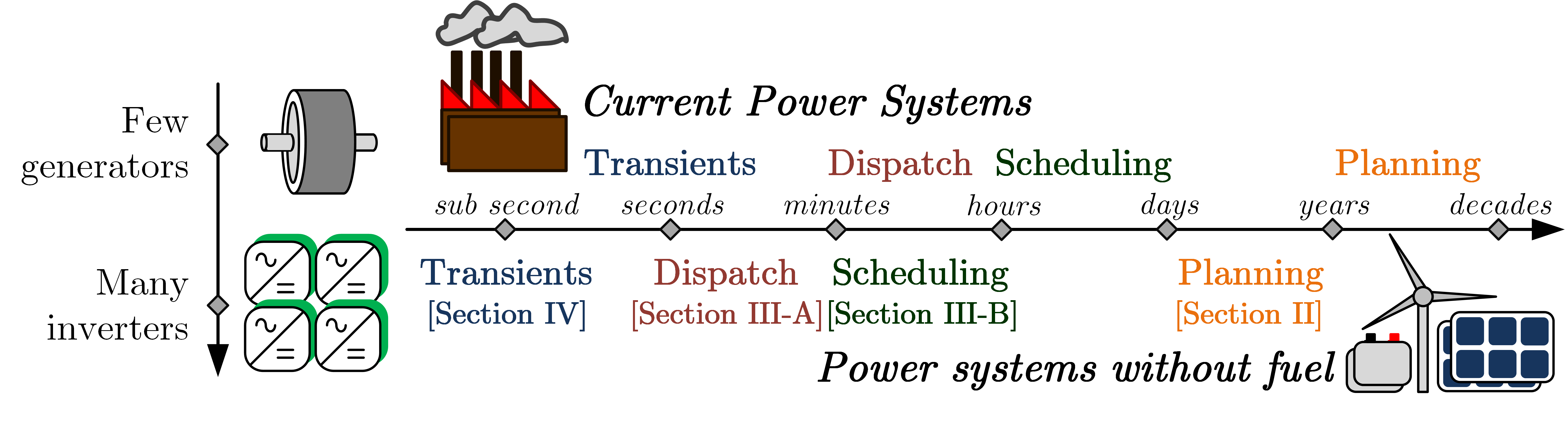
Figure 1: No-fuel power systems will have fundamentally different spatio-temporal characteristics. Time scales governing operations and control will shrink, and energy-conversion interfaces will be distributed in form and function.

It may well be some time before continental-scale portions of power systems are fully on the soft energy path. However, there are a number of encouraging small-scale examples, a few of which we list below:

• Scotland exceeded its target of 31% renewable electricity production by 2011, and has established targets of 50% and 100% by 2015 and 2020, respectively [8].

• Following a destructive fire, the Caribbean island of Bonaire now aims to generate all of its electricity from renewables [9], about 45% of which will be wind and the remainder biofuel or biomass. Geographical remoteness makes local renewable production highly pragmatic for small island power systems [10].

• Following a nuclear disaster in 2011, the Fukushima prefecture in Japan established 100% renewable electricity production as their target for 2040 [11].

• Portugal, which has no established companies in fossil or nuclear fuel production [12], aims to have 60% renewable electricity production by 2020 [13].

I-B Setup and organization

In this paper, we attempt to broadly discuss the implications of fully transitioning electric power systems to a no-fuel future. We implicitly take the virtues of the soft energy path as given and assume almost $100\%$ renewable power production to be a viable future for a large share of power systems. In this regard, our main objective is to better understand power systems without fuel as a limiting case to help plan for an energy future that is potentially very different from the present.

By renewable, we primarily connote wind, solar, wave, and hydroelectric power production, but also allow for sustainable low-fuel, low-pollution resources like geothermal energy and fuel cells. Because we are interested in both all-renewable and almost all-renewable power production, we allow for occasional instances of these resources that contradict our setup. For example, pumped hydro and concentrating solar power plants often use synchronous generators and can be in the hundreds of MW, which is much larger than most renewables; however, both technologies still have very low marginal costs and are amenable to direct current configurations. Note that the scope of the paper does not encompass nuclear generation or biomass and biofuels, the latter of which may remain useful for some non-grid connected types of energy consumers like long-distance air travel [1, 14, 15].

Throughout our discussion, we implicitly assume the existence of large stores of flexibility, by which we mean the ability to match supply and demand on all timescales and maintain stable voltages throughout the power system. The central challenge in replacing conventional fuel-based generators with renewables is finding inexpensive sources of flexibility. Presently, flexibility is achieved via reserves and regulation. Reserves balance supply and demand in the face of unpredicted load variations and contingencies, i.e., component failures. Regulation, which includes automatic generation control, automatic voltage regulation, and droop control, balances supply and demand on faster timescales and maintains stable voltage frequencies and magnitudes throughout the power system. The reader is referred to [16, 17] for comprehensive coverage of these topics. Presently, most of these services are provided by fuel-based generators. Replacing these generators with renewables simultaneously increases the need for flexibility and removes the main source of flexibility. A core obstacle is that most new sources of flexibility are still quite expensive.

Because we are taking a long-term view in this paper, we neglect the challenge of financing the procurement of new sources of flexibility, and rather assume that sufficient flexibility can be provided by the following non-fuel-based mechanisms.

• Energy storage devices like batteries, flywheels, and pumped hydro [18]. A generic model of storage is given by equations (2)–(4) in Section III-A2.

• Flexible loads enrolled in demand response programs [19, 20]. Several recent studies have shown that flexible load aggregations can provide similar services to (and are well-modeled by) storage [21, 22, 23]. For this reason, we will generically use the term storage to refer to devices like batteries and flywheels and to virtual storage from aggregations of flexible loads.

• Spilling renewable power by operating below capacity limits. The maximum power output of a wind or solar power producer depends on prevailing ambient conditions which are inherently random. Renewables are largely dispatchable up to their maximum power outputs [24, 25].

• Power electronic devices. Converter interfaces for renewables, storage [26], and direct current systems [27, 28] and FACTS devices [29, 30] can provide voltage support and regulation on fast timescales.

The remainder of the paper is organized as follows. In Section II, we discuss planning and some broader issues like couplings to other infrastructures and DC systems. We move to the steady-state timescale in Section III, where we discuss the scheduling problems of unit commitment and load-shifting, real-time dispatch, and the economics of power systems without fuel. We discuss dynamics and transient stability in Section IV. Figure 1 illustrates the paper’s organization within the motif of evolving spatiotemporal characteristics.

II Long-term planning and broader issues

In this section, we discuss planning with renewables and the broader issues of direct versus alternating current and couplings with other infrastructures.

II-A Economies of scale and geographic constraints

This section focuses on basic differences between planning with fuel-based generators and with renewables and storage. We structure our discussion around the following generic optimal planning problem.

$$\begin{array}[]{rl}\underset{x,y}{\mathrm{minimize}}&\underset{\sigma}{\mathbb{E}}\left[\displaystyle\sum_{i\in\mathcal{C}}c_{i}(x_{i},\sigma)+f(x,y,\sigma)\right]\\ \mathrm{such\,\,that}&0\leq x_{i}\leq\overline{x}_{i},\quad x_{i}\in\mathbb{Z},\\ &y\in\mathcal{P}(x).\end{array}$$ (1)

Here, $x_{i}$ represents the decision to install component $i\in\mathcal{C}$, where $\mathcal{C}$ is the set of candidate components, and $y$ is the vector of operational variables, for example, real and reactive power flows and voltage. The first constraint on $x_{i}$ represents the quantity installed, and the second constraint introduces a discrete requirement, e.g., that the number of wind turbines must be integer valued. The feasible set of operational variables depends on the installed components via $\mathcal{P}(x)$. The first term in the objective is the sum of installation costs, and the latter, the total operating cost. Because installation can span weeks to decades, the expectation of the cost is taken over $\sigma$, a vector of random variables representing uncertain future information like load growth and material and fuel costs.

Economies of scale reduce fuel-based generator costs as installed capacity increases. On the contrary, wind turbines and PV inverters are typically available at smaller ratings, often one to two orders of magnitude less than fuel-based generators in terms of watts per facility. For example, in 2013, the average U.S. coal, gas, and nuclear plant capacities were approximately $272\,\mathrm{MW}$, $85\,\mathrm{MW}$, and $104\,\mathrm{MW}$, respectively [31]. On the other hand, the Vestas V164 has the largest capacity of any individual wind turbine at $8\,\mathrm{MW}$ [32], and the average installed residential-scale PV system was $6.2\,\mathrm{kW}$ in 2012 [33]. While constructing a fuel-based generator takes around five years, wind turbines typically take a few months, and photovoltaic systems and many storage technologies need only be interconnected. Fuel-based generators are built to operate for several decades. Wind turbines are typically designed for a twenty-year lifetime [34], while PV panel components can be expected to last anywhere from five years to two decades [35, 36]. PV can be incrementally installed on daily timescales, which should be reflected in scheduling and dispatch routines.

Renewables are subject to different geographical constraints than fuel-based generators. Typical generation planning constraints may include minimal distance from population centers and proximity to water sources for cooling. On the other hand, renewables are geographically constrained by weather characteristics such as in the cases of offshore wind and desert solar power plants, which may entail significant new transmission investment [37, 38]. Similarly, accommodating rooftop PV systems in existing distribution networks calls for an upgrade in distribution-system infrastructure. In the short-term, this implies that renewables may require more transmission expansion than fuel-based generators. In the long-term, this may incentivize large power consumers to locate in energy dense regions. There are few (if any) geographical constraints on non-hydroelectric storage.

In economic terms, the above-described smaller unit sizes make planning renewable energy installations considerably less lumpy than fuel-based generators; rather than infrequently building large generators over long intervals, wind turbines and solar panels can be installed incrementally over shorter time periods. We summarize the resulting differences in the context of the optimization problem in (1) below.

• Planning renewables has lower computational complexity than fuel-based generators. For instance, because wind turbines and solar panels come in finer size increments than fuel-based generators, the sets of possible farm sizes are better approximated by continuous intervals. In (1), this means increasing the number of sizes a candidate component can take on, $\overline{x}_{i}$, and decreasing the sensitivity of the cost, $\sum c_{i}(x_{i},\sigma)+f(x,y,\sigma)$, and feasible operating range, $\mathcal{P}(x)$, on the installation variable $x_{i}$. This improves the quality of continuous approximations, and in turn, the performance of integer programming techniques like branch-and-bound [39, 40], making optimal plans easier to obtain.

• Renewables need shorter planning horizons than fuel-based generators. This leaves less time for predictions at the start of the project to deviate from reality once completed, for example due to unexpected load growth. In (1), this means reducing the variance of the random variable $\sigma$. While this may not affect the expectation of the objective, it decreases the risk by reducing the likelihood of the expected cost diverging from the realized cost. Consequently, there is less uncertainty from long planning horizons with renewables, decreasing the risk of wasted investments.

• In power systems that conduct generation expansion through market mechanisms rather than the centralized solution of mixed-integer programs (see, e.g., [41, 42]), having more numerous, smaller market participants more nearly satisfies the underlying theoretical assumptions of competitive markets [43]. In particular, renewable producers will be closer to price-takers, thus enhancing competition and easing market entry for new firms.

• On the other hand, power systems that rely on market signals to incentivize capacity expansion will likely rely increasingly on capacity payments, i.e., payments for generators to be available to deliver power in the future, and less on coordinated spot markets for energy, which currently compensate producers at the marginal cost of the highest accepted bid. “Energy only” wholesale markets (i.e., markets with only spot energy prices and without capacity payments) such as those in Texas and Alberta will probably need to be re-designed to ensure that capacity expansion continues to meet reliability requirements in the face of potentially reduced energy market revenues.

II-B Coupling to other infrastructures

In this section, we address dependencies on other infrastructures. Removing fuel-based generators decouples power systems from other infrastructures because in the envisioned no-fuel future:

• fuel does not need to be mined and transported via ship, rail, road, or pipe;

• significantly less waste (e.g., ash from coal power plants) needs to be disposed of; and

• water is not necessary for cooling, as it currently is for thermal power plants.

These decouplings further reduce planning complexity by removing considerations such as collocating fuel-based generators and desalinization plants.

Power systems without fuel will however be more coupled to the transportation and communication infrastructures. Coupling power systems to transportation through electric vehicles and trains will increase complexity, but at the benefit of decoupling transportation from the fuel infrastructure. Leveraging smart meters and employing more real-time control [45] enhances the achievable performance of power systems while introducing security and privacy vulnerabilities [46].

II-C AC versus DC and the relevance of frequency

Since the so-called “War of the Currents” of the 1880s, AC has been a core feature of power systems around the world; [47] provides an excellent historical account. Since then, the question of which would be better today has often been posed, cf. [48]. We now do so again for power systems without fuel. For cohesion, we contain our entire discussion of this issue to this section despite certain aspects like stability informing faster timescales discussed elsewhere in the paper.

First, recall the two main reasons for using AC instead of DC.

• Transformers only work with AC and until recently were the only practical solution for long-distance transmission.

• Synchronous machines can directly synchronize with AC power systems.

Today, power electronics offer alternative mechanisms for varying current to voltage ratios that are compatible with both AC and DC [49], negating the first point above. Absent synchronous generators, synchronous and induction motors are the only remaining major classes of devices that are sinusoidally excited. Electric motors make up approximately 45% of global electric power consumption, 23% of which are synchronous for a total of approximately 10% of the global load, a clear minority [50]. Almost all other loads merely tolerate AC because the unwanted effects of 60Hz oscillations are imperceptible (e.g., lighting) or because they are equipped with adaptors that locally covert to DC (e.g., computing).

The major shortcoming of DC relative to AC is at the protection level; AC faults are easily cleared because the current crosses zero 120 times per second, but DC current is constantly nonzero, leading to potentially dangerous arcing when circuits are opened. Viable protection schemes exist, especially for low-voltage settings [51], but they are more expensive than their AC counterparts. In high-voltage settings, new technologies like multi-level voltage source converters offer promising solutions [52, 53]. Since conceptual solutions already exist, we regard DC protection as a surmountable obstacle that will become more economical with future research.

The features that made AC indispensable for the power systems of the last century, voltage conversion via transformers and machine synchronization, respectively can be achieved by other means (power electronics) or serve little purpose in power systems without fuel. We list several distinct differences between AC and DC transmission systems below.

First, high-voltage DC transmission is an established technology [27, 54, 28] that is superior to AC in terms of

• only needing one rather than three phases,

• more efficient wire utilization because the RMS and peak currents are approximately the same,

• providing enhanced stability via additional controllability and physical decoupling [55, 56, 57],

• and requiring reduced communication due to amenability to decentralization [58, 59].

DC is also viewed as a conceptually superior option for small power systems such as industrial sites [60, 51] and microgrids [61, 62] because of

• improved efficiency due to decreased losses between DC sources and loads,

• absence of synchronization and reactive power considerations,

• and improved isolation from faults and failures on the main grid.

Finally, operating DC systems in steady-state is mathematically simpler than AC systems. This was part of the reason behind Edison’s opposition to AC. The modern pragmatic implication is that DC systems lend themselves to easier computations, further reducing the operational complexity of power systems. In particular, convex relaxations of DC power flow [63] are exact under more general conditions than convex relaxations of AC power flow [64, 65]. This means that solving the standard nonconvex optimal power flow is tractable in the DC case for a wider range of systems than the AC case.

Main points.

Planning renewables introduces new transmission requirements. However, planning renewables is an easier problem than planning fuel-based generators because

• renewables and storage devices come in smaller units, improving the accuracy of continuous approximations to planning problems and hence decreasing the difficulty of the associated integer programs; and

• they can be installed over shorter time periods, decreasing uncertainty from long planning horizons.

The following two considerations suggest that power systems without fuel can attain superior performance to that of current power systems.

• Power electronics and the absence of synchronous generators make DC a viable paradigm.

• With the exception of communications, power systems without fuel will be less coupled to other infrastructures, reducing complexity and enhancing robustness.

III Steady-state Operation

In this section, we discuss the effects of removing fuel-based generators on steady-state operations where bulk supply is matched to demand.

III-A Scheduling

The two main scheduling problems in power system operations are

• unit commitment, the problem of selecting when fuel-based generators are online and offline, and

• load shifting, the problem of moving energy in time via storage.

Eliminating fuel-based generators and adding renewables and storage eliminates unit commitment and increases the system’s load-shifting capability. Impacts of renewable intermittency are more pronounced on real-time dispatch, which we address in Section III-B.

III-A1 Unit commitment

Unit commitment has long been a central part of power system operations [66, 67, 17]. Unit commitment is challenging because a fuel-based generator can take hours to a day to switch between on and off states. Consequently, the attendant scheduling problem requires binary variables to indicate when fuel-based generators are on and off, and unit commitment solutions must be obtained hours to days in advance of real time. The resulting combinatorial problems are often posed as mixed-integer programs [68], which, despite the development of powerful heuristics, are NP-hard and hence difficult to solve [39, 40]. Generator reserves—idling generators kept online as insurance against failures—must also be scheduled in advance, and are usually incorporated into unit commitment routines [69, 17].

Unlike fuel-based generators, wind turbines and hydroelectric generators can go from off to maximum output in minutes due to the absence of thermal constraints [70]. Solar panels and distributed energy-storage devices that are interconnected through power electronics can engage and disengage almost instantaneously [25]. Without fuel-based generators, the most stringent of these startup and shutdown constraints amounts to a few minutes, which is essentially real-time with respect to current power system operational practices. Therefore, a major perk of eliminating fuel-based generators is the elimination of the unit commitment problem and the concomitant need to procure reserves long in advance, which in turn has the following benefits:

• The computational complexity of power system operations decreases because combinatorial scheduling problems, i.e., integer programs, do not need to be solved.

• The uncertainty resulting from scheduling fuel-based generators hours to days in advance disappears. Instead, renewables and storage can be brought online with lead times on the order of minutes. This reduces the time for predictions to deviate from reality, hence reducing the risk of inefficient decisions.

Without fuel-based generators, reserves must be supplied by storage to ensure power balance in the face of contingencies, load variations, and renewable intermittency. However, holding slack storage capacity does not incur costs in the way that fuel-based generator reserves do.

• Assuming the storage’s leakage is low (which is realistic for technologies like batteries and pumped hydro [18]), keeping a storage device on standby is essentially free. On the other hand, fuel-based generators are expensive to keep on standby due to fuel consumption and other operating expenses.

• Fuel-based generators incur opportunity costs because providing reserves limits the base-load power they can sell in energy markets. Storage incurs no such opportunity cost since it does not provide base-load power.

III-A2 Load-shifting

Load-shifting refers to using storage to extract power from the system (typically at times of low net demand) and inject power later (typically at times of high net demand).

$$s_{t+1}=\alpha s_{t}+\Delta\left(\eta_{\textrm{in}}\max\{u_{t},0\}+\eta_{\textrm{ex}}\min\{u_{t},0\}\right),$$ (2)

where $s_{t}$ and $u_{t}$ are respectively the state of charge and power injection/extraction in time period $t$, $\alpha\in[0,1]$ is the leakage over one time period, and $\eta_{\textrm{in}}\in[0,1]$ and $\eta_{\textrm{ex}}\in[1,\infty)$ are the injection and extraction losses, and $\Delta$ is the length of each time period. Typically, the state of charge, injection, and extraction are subject to energy and power capacity constraints of the form

$$0\leq s_{t}\leq C,\quad\left|u_{t}\right|\leq R,$$ (3)

Observe that the above model only contains linear constraints. If the storage has a power-electronic grid interface and is to be used for voltage support, reactive power can be included via the convex quadratic constraint

$$u_{t}^{2}+q_{t}^{2}\leq R^{2},$$ (4)

where $q_{t}$ is the reactive power into or out of the storage device. Since this model only contains convex constraints, load shifting is a fairly tractable problem that can be addressed via dynamic programming [71] or multiperiod optimal power flow  [72]; we discuss this further in Section III-B.

With the storage and power-electronics models outlined above, we can now dwell on the following generic optimal load-shifting problem.

$$\begin{array}[]{rl}\underset{p,u}{\mathrm{minimize}}&\displaystyle\sum_{t=1}^{T}\sum_{i\in\mathcal{G}}f_{i,t}(p_{i,t})\\ \mathrm{such\,\,that}&u_{i}\;\textrm{satisfies~{}\eqref{eq:storage0}--\eqref{eq:storage2}, }i\in\mathcal{S},\\ &\underline{p}_{i,t}\leq p_{i,t}-u_{i,t}\leq\overline{p}_{i,t},\;i\in\mathcal{S},\\ &p\in\mathcal{P}.\end{array}$$ (5)

The objective is the sum of production costs for all generators over the time period of interest. Load-shifting schedules can span hours ($T\approx 10$) to a few days ($T\approx 100$). A subset of nodes, $\mathcal{S}$, have storage. The second constraint represents the offset to the net supply and demand resulting from storage injections and extractions. The last constraint requires that all power quantities, $p$, be physically feasible; for example, $\mathcal{P}$ could represent the set of feasible power injections under linearized power flow and line flow limits. Note that uncertainty does not factor into our discussion of load-shifting, and is addressed later when we discuss dispatch with multiperiod optimal power flow in Section III-B.

We distinguish between three functions of load-shifting.

• Storage can flatten the net load seen by power producers. This leads to more efficient power production because the functions $f_{i,t}(p_{i,t})$, $i\in\mathcal{G}$ in (5) are approximately convex and increasing [17]. Storage profits from this practice by arbitraging price differences over time. Without fuel-based generators, system efficiency is far less dependent on output levels, and thus the price of power may not change in time; we discuss this further in Section III-C. As such, we see little benefit from load-shifting for efficiency in power systems without fuel.

• Load shifting can move power to accommodate production capacities. This makes the second constraint in (5) easier to satisfy, thus enlarging the feasible range of operation. Much of present-day load-shifting of this type accommodates the startup and shutdown constraints of fuel-based generators. For example, flattening load makes nuclear power plants more economical by enabling them to continuously operate near their capacity limit and avoid going offline [73]. In power systems with high dependence on non-dispatchable resources like wind and solar, more load-shifting is needed to match supply and demand [74].

• Load-shifting can be used to reduce peak consumption levels, in turn reducing system capacity requirements. In (5), this means attaining feasibility without changing each $\overline{p}_{i,t}$, hence reducing component installation costs in (1). This sort of load-shifting, also known as peak-shaving, is useful with and without fuel-based generators.

Much of the storage necessitated by renewables provides services other than load-shifting such as power balancing and regulation, which are discussed in Sections III-B and IV.

Finally, a key difference between load shifting and unit commitment is that the load-shifting decisions can be implemented in near real time. This is because storage needs only a few seconds to change its power output while a fuel-based generator may take half of a day to turn on or off. Consequently, although load-shifting schedules can span more than a day, the attendant computations and decisions can be made just prior to real-time. For instance, future schedules could be continually updated in the fashion of model predictive or receding horizon control [75] by solving (5) every five minutes.

Main points.

Unit commitment and advance procurement of reserves are not necessary without fuel-based generators. Load-shifting is critical to accommodating non-dispatchable supply and reduce capacity requirements. Although load-shifting schedules can span days, load-shifting actions can be implemented in near real-time. Consequently, there is little (if any) need for day-ahead scheduling in power systems without fuel.

III-B Dispatch

Power system operators continually update device settings such as transformer tap positions, the reactive power outputs of FACTS devices, and, most importantly, the real power outputs of power producers. These dispatch decisions are made by solving an optimal power flow, which minimizes instantaneous operating costs subject to the resulting power flow satisfying various network constraints. Optimal power flow can be solved at higher physical resolutions than unit commitment because the continuous nonconvexities arising from power flow constraints admit accurate linear and convex conic approximations [64, 65, 76]. As mentioned in Section II-C, DC is a viable basic paradigm of power systems without fuel, which would lead to more power transfers and slightly more tractable optimal power flow computations [63].

A generic multi-period optimal power flow routine can be written in the form

$$\begin{array}[]{rl}\underset{p,q,u,v}{\mathrm{min}}&\underset{\sigma}{\mathbb{E}}\left[\displaystyle\sum_{t=1}^{T}\sum_{i\in\mathcal{G}}f_{i,t}(p_{i,t},\sigma)-\sum_{i\in\mathcal{L}}d_{i,t}(p_{i,t},\sigma)\right]\\ \mathrm{s.t.}&\{p,q,u,v\}\in\mathcal{P}.\end{array}$$ (6)

Here, $p$ is real power, $q$ reactive power, $v$ voltage, and $u$ represents storage as in (5); $T$ is the total number of time periods, e.g., 48 hours would be appropriate if multi-day wind events were an issue. The function $f_{i,t}(p_{i,t},\sigma)$ is the cost of producing $p_{i,t}$ at time $t$ if $i$ is in the set of generators, $\mathcal{G}$; and $d_{i,t}(p_{i,t},\sigma)$ is the utility of consuming $p_{i,t}$ at time $t$ if $i$ is in the set of loads, $\mathcal{L}$. The expectation is over $\sigma$, a random variable that captures, e.g., uncertainty in demand or renewable output. The constraint represents all of the system physics, including power flow and storage constraints. We remark that (6) is a generalization of the load-shifting problem (5), and that load-shifting schedules can be computed alongside other dispatch decisions within multi-period optimal power flow. Within the planning problem (1), the optimization problem (6) would be embedded in $d(x,y,\sigma)$ and $\mathcal{P}(x)$, albeit in a simplified form for tractability.

The dominant portion of the generator cost curves, $f_{i,t}(p_{i,t},\sigma)$, $i\in\mathcal{G}$, are the fuel costs. These functions are approximately convex and increasing because generators tend to burn fuel less efficiently at higher power output levels [17]. In North America, the $f_{i}(p_{i})$ are usually based on supply functions associating prices with output-power levels, which are declared by generators prior to dispatch. Currently, the load utility curves, $d_{i}(p_{i})$, $i\in\mathcal{L}$, are often only present in unit commitment and not optimal power flow because loads have little real-time elasticity. This is changing with the advent of demand response [77, 78].

System operators will seek to optimally dispatch power systems without fuel, for instance, by setting storage charging and discharging schedules, choosing the set-points of power electronic devices, and adjusting the power captured from renewables, e.g., by adjusting wind turbine blade pitch and the incidence angle of PV arrays. To accommodate large-scale production by renewables, (6) must be modified in the following four ways:

• Uncertainty from forecast errors due to renewable intermittency must be included.

• Dynamic constraints from storage, e.g., (2)–(4), and serial correlations in renewable intermittency must be included.

• The presence of numerous dispatchable resources like inverters and storage in low-voltage distribution systems may necessitate decentralization.

• New objectives are needed to replace fuel costs.

We discuss these four issues in the order listed.

III-B1 Uncertainty

Renewable intermittency adds significant uncertainty to dispatch decisions in the form of forecast errors. Of course, lower levels of uncertainty from loads and contingencies (e.g., line outages) have always been present in power system operations, cf. [79]. As mentioned in Section I-B, wind and solar power plants can be operated such that they are dispatchable up to their maximum power outputs, which are determined by random factors like wind speed and solar intensity.

The following are a few well-known, contemporary approaches to incorporating uncertainty into optimal power flow routines. Each approach would be implemented in the context of (6) by suitably modifying $\sigma$ and its distribution and in the feasible set $\mathcal{P}$.

• The chance constraint is a tool from stochastic programming [80, 81] that requires the probability of an event to be above or below a certain level, for example, that the probability a collection of renewables satisfies the net load is greater than $0.99$. While generally nonconvex, some chance constraints can be cast as linear [80] and second-order cone constraints [82], the latter of which have been used as a tractable basis for chance-constrained optimal power flow [83].

• The scenario approach is an alternative approximation to stochastic programming in which scenarios are sampled from probability distributions and used to estimate the feasibility of chance constraints. The scenario approach has also seen wide application in power systems [84], particularly in unit commitment routines [85].

• Robust optimization is a more tractable, less descriptive approach to uncertainty modeling compared to stochastic programming, which specifies uncertain sets without probability distributions [86]. Robust optimization has also proven useful in power systems [87], again particularly with unit commitment [88].

We remark that from a computational perspective, replacing fuel-based generators with renewables entails replacing intractable discrete constraints with uncertainty. While significant theoretical and empirical work is needed to quantify this tradeoff, this hypothesis appears to be reasonable for the following reasons:

• Renewable uncertainty admits more modeling choices than discrete unit commitment constraints, which essentially must always be modeled as integer variables.

• Models of uncertainty are more amenable to tractable (convex) approximations. Most approaches to combinatorial optimization retain discrete modeling.

III-B2 Dynamic constraints

Flexibility from storage and demand response is necessary to accommodate renewable intermittency. Because both resources have finite energy capacity, dynamic modeling is necessary to describe the evolution of its state of charge. This includes both load-shifting as discussed in Section III-A and power balancing to match supply and demand on sub-minute timescales. Because the basic storage constraints, (2)–(4), are linear and convex quadratic, optimal storage decisions can be obtained alongside standard dispatch decisions via multiperiod optimal power flow [72]. A multiperiod optimal power flow routine like (6) is a sequence of single-period optimal power flow routines that are coupled period-to-period by storage dynamics like (2)–(4) and other constraints such as ramp limits on power production. Multiperiod optimal power flow has approximately $NT$ variables and $MT$ constraints, where $N$ and $M$ are the number of variables and constraints in each individual period, and $T$ is the number of periods. Despite the increased number of variables and constraints, fundamentally, multiperiod optimal power flow is no more complex than ordinary optimal power flow, e.g., a multiperiod version of a second-order cone optimal power flow is still a second-order cone program [76]. A useful implication of this is that stochastic and robust optimal power flow models can be extended to the multiperiod case to accommodate serial correlations in wind speeds and incident solar irradiance.

A recent alternative to multiperiod optimal power flow is risk-limiting dispatch [90, 91], which is based on dynamic programming rather than convex optimization. Risk-limiting dispatch offers less modeling versatility than multiperiod optimal power flow, but in return produces policies instead of trajectories, which better accommodate uncertainty by specifying a decision for any realization of the system state [92].

III-B3 Decentralization

We now briefly discuss decentralization. For many years, only generators and other transmission level devices could actively change their set points in response to commands. Now, components in low-voltage distribution systems like PV inverters and small energy storage devices must actively change their set points to accommodate uncertainty from distributed renewable generation; note that this largely overlaps with the paradigm of distributed generation [6, 93]. Computational and communication-based limitations will likely prohibit system operators from centrally operating these devices. In this case, decentralized optimal power flow algorithms will be needed to dispatch devices with limited communications. Numerous approaches already exist, including consensus-based approaches [94] and the alternating direction method of multipliers [95, 96]. While decentralization must always entail a performance loss relative to the centralized case and has long been a mathematically challenging topic, the online computational requirements of practical decentralized algorithms are generally lower than their centralized counterparts simply because they involve breaking a large problem into smaller pieces. We revisit decentralization from the perspective of real-time control on faster timescales in Section IV.

III-B4 Dispatch criteria

Lastly in this section, we address the fact that renewables operate at zero marginal cost, i.e., once they are built, the power they produce costs very little [97]. We discuss the economic implications of this feature in Section III-C. After removing fuel-based generators from power systems, only the load utilities remain in the objective of multiperiod optimal power flow, (6), which are often not present in real-time dispatch routines. Because current power system operations are almost entirely centered around minimizing fuel consumption, alternative objectives are needed for power systems without fuel; a few possibilities are listed below. Note that we do not consider resistive losses to be a valid objective due to the low marginal cost of the power itself.

• Maintenance is the next most significant monetary cost that explicitly depends on how the system is dispatched. Maintenance and health monitoring in power systems are well-studied topics, e.g., for pumped hydro storage [98], wind turbines [99, 100], PV and storage systems [101, 102, 103], and transmission lines [104, 105]. There is also a well-developed literature on maintenance theory [106].

• Reliability-based objectives minimize the risk of component failures and instability [79]. We classify reliability as a non-monetary objective because it is difficult to ascribe explicit costs to potential failures. A reliability objective might include nuanced considerations such as probabilistic failures, or could be as simple as minimizing the maximum current-to-capacity ratios across the network [107]. The latter can be written as

  $$\sum_{i}w_{i}\left(\frac{x_{i}}{X_{i}}\right)^{2},$$ (7)

  where $x_{i}$ and $X_{i}$ are the usage and capacity of component $i$, e.g., the apparent power flow through and thermal capacity limit of a transmission line or power electronic converter, and $w_{i}$ a positive weighting factor.

• Power quality refers to keeping the system voltage close to its nominal profile on steady-state and transient timescales [108]. Power quality affects the performance and lifetime of grid-connected devices. We also classify power quality as non-monetary because the costs of voltage fluctuations are difficult to quantify.

• Presently, most real-time dispatch routines take the loads across the system as a fixed set of parameters. Demand response enables loads to modify their aggregate consumption in real-time in response to the system’s state and needs. An aggregation of active loads could submit a bid curve to the system operator associating its range of power consumptions with varying utility levels. This could be a monetary bid, cf. [109].

The first three objectives overlap significantly. For example, improved reliability should improve power quality and vice versa while reducing maintenance costs. These objectives are also closely tied to transient behaviors; for example, increasing the real power output from a solar power plant will cause more disturbances in that part of the network, in turn impacting the transient stability of the system. We further discuss this coupling in Section IV. As a general rule, we suggest that the objective not introduce complexities beyond the constraints needed to accurately represent the physics, e.g., an objective that must be evaluated by Monte Carlo integration would compromise the tractability of the overall dispatch routine.

Main points.

Dispatching power systems without fuel will differ in four ways from current practices.

• Forecast errors from renewable intermittency must be accounted for with uncertainty modeling.

• Multiperiod optimal power flow must be used to model the dynamics of storage and serial correlations in renewable inputs.

• In some cases, distributed resources will need to be operated in a decentralized fashion.

• New objectives are required to replace fuel costs in dispatch routines.

III-C Economics

In this section, we discuss the economics of supplying power with only renewables. A large and growing body of literature addresses the assimilation of renewables into the current market framework, see e.g. [97]. The reader is referred to [110, 111] for thorough expositions of power system economics. While these techniques are effective when some of the total power is produced by fuel-based generators, we believe that there is room for new perspectives when all of the power is from renewables.

Presently, most producers in North America have several revenue streams.

• A bilateral contract is low risk, long-term mechanism for a producer to sell a fixed quantity of power to a consumer at a price agreed upon ahead of time.

• Producers can sell power in spot markets at nodal prices that are the dual variables of optimal power flow with a fuel cost objective. This approach was pioneered in [112] and is a conceptual application of the Fundamental Theorems of Welfare Economics [43]. An attractive quality of nodal prices is that they are outputted by optimal power flow routines and represent the sensitivity of the objective to incremental changes in power levels. Spot markets provide competitive venues for buying and selling power, which fill the essential roles of adding liquidity and driving down prices of bilateral contracts.

• Producers are paid for providing flexibility under the names reserves and regulation. Reserve providers are often paid through call options in which they receive capacity payments for holding idle capacity on standby and energy payments if they are actually called on [113, 114, 115]. Resources are also paid for providing regulation; the form of these payments has been a topic of recent debate [116, 117].

• System operators or load serving entities sometimes make long-term capacity payments to power producers for being present to bid in markets and provide power over periods of years. These payments encourage construction of new generation. As discussed at the end of Section II-A, capacity payments could play a large role in power systems without fuel. Note, however, that their implementation would likely require a redefinition of the notion of capacity to accommodate the random maximum outputs of renewable power sources.

Bilateral contracts and spot markets are core features of today’s power systems and should be present in some form if power systems without fuel are to be competitive. Flexibility is costly and essential to the reliability of power systems without fuel and hence should also be represented in markets.

Here, we focus on spot markets because they are at the foundations of current power markets but are questionable in their current form for power systems without fuel. The core challenge lies in the fact that power systems without fuel have high fixed costs and low marginal costs, much like the internet, software, and digital media [118, 119]. We discuss the economics of regulation further in Section IV-D2.

Because there are no fuel costs, employing nodal pricing as is would simply result in all prices being equal to zero. The fuel cost objective in (6) could hypothetically be replaced with one or a combination of the objectives discussed in Section III-B such as maintenance costs, and nodal prices could be defined as usual. In this case, any new objective in (6) must be monetary for the dual multipliers to have valid price interpretations; if the objective is not monetary, then the dual multipliers are simply the sensitivities of the optimal objective and not marginal cost-based prices. We must, however, ask whether this is appropriate for power systems without fuel. The following are three fundamental issues.

• Time-varying nodal prices reflect the instantaneous physical efficiency and hence marginal cost of operating the power system, which currently varies on a minute-to-minute basis. This results in generators being paid according to their efficiency, and, under dynamic pricing [122], incentivizes efficient power consumption over time. Although demand and system capacity will vary in time, it is not clear that the marginal cost of operating power systems without fuel varies on a minute-to-minute or even hourly basis.

• It is straightforward to map generation levels to the cost of fuel consumption, making it relatively easy to audit bidding by fuel-based generators. The costs of maintenance, reliability, and power quality are harder to quantify and hence harder to audit. Bidding mechanisms based on these costs may consequently be more susceptible to market power and gaming.

• Demand-side bidding alone cannot account for the cost of supplying power, but rather only what consumers are willing to pay, hence removing producer input from the price-setting process. Such an arrangement can lead to excessively small payments to producers. For example, if we model such demand-side bidding with supply function competition [123, 124], it is trivially a pure strategy Nash equilibrium for all bids to be zero, thus rendering zero payments.

Due to the above issues, it is our stance that replacing fuel-based generators with renewables warrants a rethinking of power markets.

Main points.

The low marginal and high fixed costs of renewable power production makes the current nodal pricing framework dubious for power systems without fuel. The development of new market mechanisms will rely on accurately quantifying the cost of operating power systems without fuel on all timescales. Since these costs may be based on a number of complex and hard to audit factors, market power and gaming are important considerations.

IV Transient behavior

Several challenges will need to be addressed from modeling, analysis, and control perspectives as we embrace the transition from electromechanical energy-conversion interfaces (synchronous machines) delivering power from thermal sources (coal, nuclear, gas) to semiconductor-based energy conversion interfaces (power-electronic converters) delivering power from renewable resources (wind and solar). The main challenges in this context are the following.

• The system dynamics in the envisioned power systems without fuel are not dominated by mechanical generator rotor inertias. Apart from electrochemical and electromechanical energy storage devices (batteries and flywheels, respectively) power-electronic energy conversion interfaces offer limited inertia innately.

• Steady-state dispatch decisions now have greater effect on transient stability. For instance, procuring a large amount of power from a PV power plant also increases the magnitude of the disturbances it contributes.

• Dynamics of fast-switching power converters present imposing analysis challenges. Quasi-stationary phasor representations of electrical-network voltages and currents that are commonly used in bulk power systems lack the required modeling fidelity in power systems without fuel.

While one could argue that with the reduced mechanical inertia, a no-fuel power system is likely to be more sensitive to disturbances, conceivably, there is also more control flexibility since power-electronic interfaces can act on much faster timescales compared to synchronous generators. Next, we offer perspectives on how modeling, analysis, and control frameworks will need to be revised in a no-fuel future.

IV-A Modeling

Problems related to stability in power systems dominated by synchronous generators have received significant attention over the years. A classification of different stability notions and links to reliability and security is available in the report [125]. From the generation perspective, stability issues are typically studied for a networked collection of synchronous generators, with nodal dynamics modeled by the ubiquitous swing equations. Adopting a standard one-axis model for synchronous generators in the power system [126], the swing equations are given by

$$\frac{\mathrm{d}\delta}{\mathrm{d}t} =\omega-\omega_{\mathrm{synch}},$$

$$\frac{\mathrm{d}\omega}{\mathrm{d}t} =\frac{1}{M}\left(P_{\mathrm{mech}}-P_{\mathrm{elec}}-D(\omega-\omega_{\mathrm{synch}})\right),$$ (8)

where $\delta$ and $\omega$ are the rotor angle and speed, $\omega_{\mathrm{synch}}$ is the synchronous speed, $M$ and $D$ are the inertia constant and damping coefficients, $P_{\mathrm{mech}}$ is the mechanical-input power, and $P_{\mathrm{elec}}$ is the electrical power that flows into the network.

Dynamic models for power-electronic inverters are (circuit) topology and application dependent, and difficult to abstract in a convenient analytical form akin to the ubiquitous swing equations. This is particularly due to the following reasons:

• digital control methods that are typically employed in power-electronics circuits involve state-machine-type or look-up-table-based algorithms that are difficult to encode as dynamical systems;

• the utilization of switching power semiconductor devices in power electronic systems implies that switching-time-scale behavior is only well modeled by hybrid automata for which scalable simulation platforms are lacking;

• characteristics of renewable power sources and energy storage devices are nonlinear, technology specific, and use proprietary control algorithms that are not readily accessible in the literature.

The challenges mentioned above have been tackled with modeling strategies that include: virtual prototyping [127], reachability analysis [128], and sampled data modeling and control for power-electronics circuits [129, 130, 131].

IV-B Analysis

In their original form, dynamical models that capture the electromechanical behaviors of synchronous generators in a power network are described by differential algebraic equations. Algebraic equations are introduced from real- and reactive-power-balance conditions for nodes in the electrical network. Given the lack of numerical-simulation, stability-analysis, and controller-design methods for DAE models, it is common to resort to reduced models of the electrical network when analyzing a collection of synchronous generators. These reduced models are typically composed of nonlinear ODEs and are recovered by eliminating the algebraic power-flow equations. A variety of electrical-network model reduction methods have been developed for bulk power systems [132]. To illustrate the limitations of existing approaches and outline future directions, we focus the subsequent discussion (without loss of generality) on Kron reduction.

Given an electrical network with a set of pre-specified terminals, Kron reduction recovers an electrically equivalent circuit retaining terminal nodes and eliminating non-terminal nodes [133, 134]. Kron reduction is accomplished by taking the Schur complement of the admittance matrix. In general, encoding network interactions through the admittance matrix is only possible when we rely on quasi-stationary sinusoidal-steady-state representations for the electrical network variables [135, 136, 137, 138, 139]. However, such quasistationary models admittedly lack the fidelity required to capture network transient behaviors at faster than AC-cycle time scales. Therefore, with regard to analysis of large networks of interconnected inverters, there is a pressing need to develop scalable model-reduction methods that can be applied across a wide spectrum of time scales. Noteworthy efforts in this direction are time-domain Kron reduction methods [140, 141].

IV-C Feedback Control

Frequency across the bulk power system is, to the first order, backed up by the mechanical inertia on offer from the synchronous generators. In particular, notice from (IV-A) that variations of frequency to load fluctuations, i.e., $P_{\mathrm{elec}}$ are inversely related to the generator mechanical rotor inertia. As such, power imbalances in synchronous generators directly translate to variations in electrical frequency. This fundamental relationship underlies turbine-governor control (at the generator level) and load frequency control (at the system level). In a future power system dominated by power-electronics interfaces, mechanical inertias will no longer be direct proxies for nodal frequency dynamics across the electrical network. The limited inertia on offer in power-electronics inverters is that provided by inductive and capacitive filter elements; and therefore without fuel-based generators, electrical physics can be expected to dominate at even faster timescales. The role of feedback control in this setting is magnified, and next-generation distributed-control algorithms will play an important role of maintaining stable voltages and frequencies in a network of interconnected power electronic inverters.

In the present generation of power-electronics inverters intended for grid-tied operation, controllers are designed with the implicit assumption of the existence of a stiff voltage source. The main role of inverters in this setting is to regulate the delivery of real and reactive power. This is the so-called grid-following control paradigm. Recognizing the inevitable transition to a network with a high penetration of power-electronics inverters, there has been resurgent interest in control methods that seek to regulate terminal voltages and frequencies in the absence of a stiff grid voltage. These approaches have been referred to as grid-forming controls. Efforts in this direction are largely based on the so-called droop control [142]. Inspired by the operation of synchronous generators in bulk power systems, the premise of droop control is to linearly trade off terminal voltage and frequency versus active and reactive power. To leverage the increased control capabilities offered in fast-acting power-electronics inverters, recently there has been some interest in the development of time-domain control methods that directly act on time-domain waveforms and do not assume sinusoidal steady-state operation as is done in droop control. System-theoretic methods have outlined conditions under which frequency-synchronized electrical variables can be maintained across the network with droop control [142] and time-domain approaches [143, 144]. Extending these analytical methods to accommodate a variety of energy-conversion interfaces as well as fuel-based synchronous generators is, albeit challenging, critical to understand the implications of high penetrations of power-electronics inverters.

IV-D Coupling between the transient and steady-state timescales

The spatiotemporal characteristics of power systems without fuel are fundamentally different from present bulk power systems. In particular, the generation and load are closely collocated, largely intermittent, and vary at faster timescales. This aspect motivates the development of new approaches to system management: hierarchical operational practices that enforce a strict time-scale separation between energy management and real-time control are incompatible with the form and function of no-fuel power systems.

Traditionally, network-wide energy management, e.g., optimal power flow and load-shifting, has been designed independently from feedback control mechanisms which track set-points from energy management systems, e.g., automatic generation control and droop control. This approach is based on the separation between steady-state (seconds to minutes) and transient (sub-cycle to seconds) timescales. In power systems without fuel, adopting this time-scale separation to guide optimization and control is questionable for the following reasons:

• Timescale separation is merely a simplifying approximation; designing energy management and feedback mechanisms with regard to both timescales will result in better performance [145]. Moreover, increasing the frequency at which energy management is executed will also improve performance. Improved computational capabilities make such unified designs viable.

• The dispatch of variable wind and solar power sources strongly influences the location and magnitude of disturbances, in turn influencing the system’s transient behaviors and regulation needs. Hence, decisions at the steady-state timescale strongly influence performance at the transient timescale.

In this section, we discuss the implications of jointly addressing the steady-state and transient timescales.

IV-D1 Feedback control and energy management

The goal of feedback control is to maintain stable AC waveforms (uniform voltages and frequency) across the network in spite of variations in sources, loads, and exogenous disturbances. The objective of energy management is to provide set-points to the real-time inverter controllers such that in steady-state, power losses and voltage deviations are minimized and economic benefits to end users are maximized.

Several approaches can therefore be adopted to steer the operating point of a power system without fuel to an energy management routine’s solution. One solution strategy that has received significant attention in the literature is to synthesize controllers that seek saddle points of Lagrangian functions corresponding to the network-optimization problems, and then integrating these optimization-based controllers with existing real-time controllers. The general strategy of synthesizing dynamical systems to solve convex optimization problems goes back to the seminal work of [146], and in recent years, it has received increased attention in the control systems community in light of several motivating applications [147, 148, 149, 150, 151, 152, 153, 154]. While many synthesis approaches have been put forth, one that is conceptually straightforward is to formulate dynamical systems (the states of which are proxies for Lagrange multipliers) which evolve in a gradient-ascent-like fashion towards the optimal dual solution [151]. Reference inputs for the physical-layer system are then derived from these optimization-based dynamical states. Since these controllers are formulated to dynamically seek the Karush-Kuhn-Tucker (KKT) conditions for optimality, they have been referred to as dynamic KKT controllers [150, 151].

IV-D2 Economics

Steady-state dispatch influences the location of disturbances in power systems without fuel, which in turn influences which resources will be tapped for regulation. The fast adjustments involved in providing regulation, e.g., rapidly cycling the state of charge of a battery, factor significantly into maintenance costs. As discussed in Sections III-B4 and III-C, these maintenance costs may play a significant role in the steady-state dispatch and economics of power systems without fuel. Hence, not only must energy management and feedback control mechanisms be jointly designed, but economic mechanisms must also take into account costs incurred on transient time scales.

We now comment on who should bear the cost of regulation. Historically, most disturbances have been the result of natural load variations and component failures. Load-following handles the first type of disturbance and should be paid for by the loads. Failures, however, are the result of machine breakdowns and exogenous factors like trees and lightning. Failures are only problematic on fast timescales because loads require uninterrupted power. Consequently, it is the responsibility of both the component owner and loads to pay the cost of failures, cf. [155, 156]. Such costs are often termed negative externalities because they are not clearly attributable to the actions of a specific market participant. In his seminal work, Coase identified such scenarios as problems of social cost and concluded that an appropriate division of costs can be obtained by negotiation between all affected market participants [157]. Disturbances from variable renewable power production are also negative externalities because the incurred cost would be zero either if renewables did not create disturbances or if loads did not require steady power. Hence, the cost of disturbances from renewables should be borne by both renewables and the loads they serve. The design of such cost allocation mechanisms is an important research topic in power system economics.

Main points.

Adoption of semiconductor-based power-electronics interfaces in power systems without fuel will necessitate development of new modeling, analysis, and control schemes. The following are some specific challenges.

• Inverter controllers will evolve to realize grid-forming controllable voltage sources as compared to grid-following current sources.

• Management schemes that bridge the temporal gap between real-time control and energy management are necessary to realize the full potential of responsive power-electronics interfaces.

• Maintenance of resources providing fast regulation may represent a major operational cost in power systems without fuel. New economic mechanisms may be necessary to represent these costs in markets on slower timescales.

V Summary

Climate change and the finiteness of fossil fuels make it viable that many future power systems could run entirely without fuel. Considerable technical and economic challenges lie between present-day power systems and power systems without fuel. Foremost, the intermittency of renewables entails that new sources of flexibility like storage and demand response must become more cost-effective for removing all fuel-based generation to be feasible. A new array of optimization and control algorithms must then be developed to ensure the safe and efficient operation of power systems without fuel. Complementary economic mechanisms that incentivize proper behavior and investment and which are robust to market abuse must also be developed. While daunting, we regard these challenges to be surmountable through research, technological development, and policy.

We believe that power systems without fuel will differ substantially from fuel-based power systems beyond environmental benevolence and sustainability. Many of these differences stem from the facts that all timescales are shrinking, and that there will be numerous small components instead of a few large components. Some of these differences translate to genuine advantages, including closer to real-time decision-making with more accurate information and the viability of a predominantly DC infrastructure, to name a few.

References

- [1] D. MacKay, Sustainable Energy - without the hot air. Cambridge University Press, 2008. [Online]. Available: http://www.withouthotair.com/
- [2] J. Tester, E. Drake, M. Driscoll, M. Golay, and W. Peters, Sustainable Energy: Choosing Among Options. MIT Press, 2012.
- [3] A. B. Lovins, “Energy strategy: the road not taken,” Foreign Affairs, vol. 55, p. 65, 1976.
- [4] A. Lovins, Reinventing fire: Bold business solutions for the new energy era. Chelsea Green Publishing, 2013.
- [5] M. Z. Jacobson and M. A. Delucchi, “Providing all global energy with wind, water, and solar power, part i: Technologies, energy resources, quantities and areas of infrastructure, and materials,” Energy Policy, vol. 39, no. 3, pp. 1154 – 1169, 2011.
- [6] T. Ackermann, G. Andersson, and L. Soder, “Distributed generation: a definition,” Electric Power Systems Research, vol. 57, no. 3, pp. 195 – 204, 2001.
- [7] R. Lasseter, “Microgrids,” in Power Engineering Society Winter Meeting, 2002, vol. 1, 2002, pp. 305 – 308.
- [8] T. Scottish Government, “2020 routemap for renewable energy in Scotland – update,” 2013. [Online]. Available: http://www.scotland.gov.uk/Resource/0044/00441628.pdf
- [9] “Caribbean island ditching diesel in favor of renewable energy,” 2015. [Online]. Available: http://cleantechnica.com/2015/01/09/caribbean-island-ditching-diesel-favor-renewable-energy/
- [10] M. Ilic, L. Xie, and Q. Liu, Engineering IT-Enabled Sustainable Electricity Services: The Tale of Two Low-Cost Green Azores Islands. Springer Science & Business, 2013, vol. 30.
- [11] T. D. Couture and A. Leidreiter, “How to achieve 100% renewable energy,” 2014. [Online]. Available: http://worldfuturecouncil.org/fileadmin/user_upload/Climate_and_Energy/Cities/Policy_Handbook_Online_Version.pdf
- [12] D. Reiche and M. Bechberger, “Policy differences in the promotion of renewable energies in the EU member states,” Energy Policy, vol. 32, no. 7, pp. 843 – 849, 2004.
- [13] G. Krajačić, N. Duić, and M. da Graça Carvalho, “How to achieve a 100% RES electricity supply for Portugal?” Applied Energy, vol. 88, no. 2, pp. 508 – 517, 2011. [Online]. Available: http://www.sciencedirect.com/science/article/pii/S0306261910003703
- [14] T. Searchinger, R. Heimlich, R. A. Houghton, F. Dong, A. Elobeid, J. Fabiosa, S. Tokgoz, D. Hayes, and T.-H. Yu, “Use of u.s. croplands for biofuels increases greenhouse gases through emissions from land-use change,” Science, vol. 319, no. 5867, pp. 1238–1240, 2008.
- [15] P. S. Nigam and A. Singh, “Production of liquid biofuels from renewable resources,” Progress in Energy and Combustion Science, vol. 37, no. 1, pp. 52 – 68, 2011.
- [16] P. Kundur, Power system stability and control. McGraw-Hill Professional, 1994.
- [17] A. J. Wood and B. F. Wollenberg, Power generation, operation, and control, 3rd ed. Wiley, 2013.
- [18] A. Castillo and D. F. Gayme, “Grid-scale energy storage applications in renewable energy integration: A survey,” Energy Conversion and Management, vol. 87, no. 0, pp. 885 – 894, 2014.
- [19] D. Callaway and I. A. Hiskens, “Achieving controllability of electric loads,” Proceedings of the IEEE, vol. 99, no. 1, pp. 184–199, Jan. 2011.
- [20] P. Palensky and D. Dietrich, “Demand side management: Demand response, intelligent energy systems, and smart loads,” Industrial Informatics, IEEE Transactions on, vol. 7, no. 3, pp. 381–388, 2011.
- [21] J. Mathieu, S. Koch, and D. Callaway, “State estimation and control of electric loads to manage real-time energy imbalance,” Power Systems, IEEE Transactions on, vol. 28, no. 1, pp. 430–440, 2013.
- [22] A. Nayyar, J. A. Taylor, A. Subramanian, D. S. Callaway, and K. Poolla, “Aggregate flexibility of collections of loads,” in Decision and Control (CDC), IEEE 52nd Annual Conference on, Dec. 2013, pp. 5600–5607, invited.
- [23] H. Hao, B. Sanandaji, K. Poolla, and T. Vincent, “Aggregate flexibility of thermostatically controlled loads,” Power Systems, IEEE Transactions on, 2014.
- [24] F. D. Bianchi, H. De Battista, and R. J. Mantz, Wind turbine control systems: principles, modelling and gain scheduling design. Springer Science & Business Media, 2006.
- [25] M. R. Patel, Wind and solar power systems: design, analysis, and operation. CRC Press, 2006.
- [26] J. Carrasco, L. Franquelo, J. Bialasiewicz, E. Galvan, R. Guisado, M. Prats, J. Leon, and N. Moreno-Alfonso, “Power-electronic systems for the grid integration of renewable energy sources: A survey,” Industrial Electronics, IEEE Transactions on, vol. 53, no. 4, pp. 1002 –1016, Jun. 2006.
- [27] J. Arrillaga, High voltage direct current transmission, 2nd ed. The Institute of Electrical Engineers, London, UK, 1998.
- [28] N. Flourentzou, V. Agelidis, and G. Demetriades, “VSC-based HVDC power transmission systems: An overview,” Power Electronics, IEEE Transactions on, vol. 24, no. 3, pp. 592–602, March 2009.
- [29] N. G. Hingorani and L. Gyugyi, Understanding FACTS: Concepts and technology of flexible AC transmission systems. Institute of Electrical and Electronics Engineers (New York), 1999.
- [30] E. Acha, C. R. Fuerte-Esquivel, H. Ambriz-Perez, and C. Angeles-Camacho, FACTS: Modelling and Simulation in Power Networks. John Wiley and Sons, 2004.
- [31] Energy Information Administration, “Existing capacity by energy source,” 2012. [Online]. Available: http://www.eia.gov/electricity/annual/html/epa\_04\_03.html
- [32] M. V. O. Wind, “The v164-8.0 mw turbine.” [Online]. Available: http://www.mhivestasoffshore.com/Products-and-services/The-Turbines/V164
- [33] L. Sherwood, “U.S. solar market trends 2012,” July 2013, [Online] Available at http://www.irecusa.org.
- [34] E. Martínez, F. Sanz, S. Pellegrini, E. Jiménez, and J. Blanco, “Life cycle assessment of a multi-megawatt wind turbine,” Renewable Energy, vol. 34, no. 3, pp. 667 – 673, 2009. [Online]. Available: http://www.sciencedirect.com/science/article/pii/S0960148108002218
- [35] C. Rodriguez and G. Amaratunga, “Long-lifetime power inverter for photovoltaic ac modules,” Industrial Electronics, IEEE Transactions on, vol. 55, no. 7, pp. 2593–2601, July 2008.
- [36] E. Voroshazi, B. Verreet, T. Aernouts, and P. Heremans, “Long-term operational lifetime and degradation analysis of p3ht:pcbm photovoltaic cells,” Solar Energy Materials and Solar Cells, vol. 95, no. 5, pp. 1303 – 1307, 2011, special Issue : 3rd International Summit on {OPV} Stability.
- [37] H. L. Willis, Distributed Power Generation: Planning and Evaluation. CRC Press, 2000.
- [38] R. Piwko, D. Osborn, R. Gramlich, G. Jordan, D. Hawkins, and K. Porter, “Wind energy delivery issues – transmission planning and competitive electricity market operation,” Power and Energy Magazine, IEEE, vol. 3, no. 6, pp. 47–56, Nov 2005.
- [39] L. A. Wolsey, Integer programming. Wiley-Interscience, 1998.
- [40] A. Schrijver, Theory of Linear and Integer Programming. John Wiley & Sons, June 1998.
- [41] F. H. Murphy and Y. Smeers, “Generation capacity expansion in imperfectly competitive restructured electricity markets,” Operations Research, vol. 53, no. 4, pp. 646–661, 2005.
- [42] J. H. Roh, M. Shahidehpour, and Y. Fu, “Market-based coordination of transmission and generation capacity planning,” Power Systems, IEEE Transactions on, vol. 22, no. 4, pp. 1406–1419, Nov 2007.
- [43] A. Mas-Colell, M. Whinston, and J. Green, Microeconomic theory. Oxford University Press, 1995.
- [44] J. Macknick, R. Newmark, G. Heath, and K. Hallett, “A review of operational water consumption and withdrawal factors for electricity generating technologies,” National Renewable Energy Laboratory, Tech. Rep., 2011.
- [45] V. Gungor, D. Sahin, T. Kocak, S. Ergut, C. Buccella, C. Cecati, and G. Hancke, “Smart grid technologies: Communication technologies and standards,” Industrial Informatics, IEEE Transactions on, vol. 7, no. 4, pp. 529–539, Nov 2011.
- [46] P. McDaniel and S. McLaughlin, “Security and privacy challenges in the smart grid,” Security Privacy, IEEE, vol. 7, no. 3, pp. 75–77, May 2009.
- [47] R. Munson, From Edison to Enron: the business of power and what it means for the future of electricity. Praeger Publishers, 2005.
- [48] D. Hammerstrom, “AC versus DC distribution systems: Did we get it right?” in Power Engineering Society General Meeting, June 2007, pp. 1–5.
- [49] R. Erickson and D. Maksimovic, Fundamentals of Power Electronics. Springer, 2001.
- [50] P. Waide and C. U. Brunner, “Energy-efficiency policy opportunities for electric motor-driven systems,” International Energy Agency, Tech. Rep., 2011.
- [51] D. Salomonsson and A. Sannino, “Low-voltage DC distribution system for commercial power systems with sensitive electronic loads,” Power Delivery, IEEE Transactions on, vol. 22, no. 3, pp. 1620–1627, July 2007.
- [52] A. Yazdani and R. Iravani, Voltage-Sourced Converters in Power Systems. Wiley - IEEE Press, 2010.
- [53] M. Merlin, T. Green, P. Mitcheson, D. Trainer, R. Critchley, W. Crookes, and F. Hassan, “The alternate arm converter: A new hybrid multilevel converter with DC-fault blocking capability,” Power Delivery, IEEE Transactions on, vol. 29, no. 1, pp. 310–317, Feb 2014.
- [54] M. Bahrman and B. Johnson, “The ABCs of HVDC transmission technologies,” Power and Energy Magazine, IEEE, vol. 5, no. 2, pp. 32–44, March 2007.
- [55] T. Smed and G. Andersson, “Utilizing HVDC to damp power oscillations,” Power Delivery, IEEE Transactions on, vol. 8, no. 2, pp. 620–627, Apr 1993.
- [56] Y. Li, C. Rehtanz, S. Ruberg, L. Luo, and Y. Cao, “Wide-area robust coordination approach of hvdc and facts controllers for damping multiple interarea oscillations,” Power Delivery, IEEE Transactions on, vol. 27, no. 3, pp. 1096–1105, July 2012.
- [57] S. Azad, R. Iravani, and J. Tate, “Damping inter-area oscillations based on a model predictive control (MPC) HVDC supplementary controller,” Power Systems, IEEE Transactions on, vol. 28, no. 3, pp. 3174–3183, Aug 2013.
- [58] J. A. Taylor and L. Scardovi, “Decentralized control of DC-segmented power systems,” in 52nd Annual Allerton Conference on Communication, Control, and Computing, 2014, invited. [Online]. Available: http://www.ele.utoronto.ca/~jtaylor/ACDC.pdf
- [59] S. Pirooz Azad, J. Taylor, and R. Iravani, “Decentralized supplementary control of multiple LCC-HVDC links,” Power Systems, IEEE Transactions on, 2015.
- [60] M. Baran and N. Mahajan, “DC distribution for industrial systems: opportunities and challenges,” Industry Applications, IEEE Transactions on, vol. 39, no. 6, pp. 1596 – 1601, Dec. 2003.
- [61] H. Kakigano, Y. Miura, and T. Ise, “Low-voltage bipolar-type dc microgrid for super high quality distribution,” Power Electronics, IEEE Transactions on, vol. 25, no. 12, pp. 3066–3075, Dec 2010.
- [62] J. Guerrero, J. Vasquez, J. Matas, L. de Vicuña, and M. Castilla, “Hierarchical control of droop-controlled AC and DC microgrids - a general approach toward standardization,” Industrial Electronics, IEEE Transactions on, vol. 58, no. 1, pp. 158–172, 2011.
- [63] L. Gan and S. Low, “Optimal power flow in direct current networks,” Power Systems, IEEE Transactions on, vol. 29, no. 6, pp. 2892–2904, Nov. 2014.
- [64] S. Low, “Convex relaxation of optimal power flow – Part I: Formulations and equivalence,” Control of Network Systems, IEEE Transactions on, vol. 1, no. 1, pp. 15–27, March 2014.
- [65] ——, “Convex relaxation of optimal power flow – Part II: Exactness,” Control of Network Systems, IEEE Transactions on, pp. 15–27, June 2014.
- [66] G. Sheble and G. Fahd, “Unit commitment literature synopsis,” Power Systems, IEEE Transactions on, vol. 9, no. 1, pp. 128 –135, Feb. 1994.
- [67] N. Padhy, “Unit commitment–a bibliographical survey,” Power Systems, IEEE Transactions on, vol. 19, no. 2, pp. 1196–1205, 2004.
- [68] M. Carrion and J. Arroyo, “A computationally efficient mixed-integer linear formulation for the thermal unit commitment problem,” Power Systems, IEEE Transactions on, vol. 21, no. 3, pp. 1371 –1378, Aug. 2006.
- [69] F. Galiana, F. Bouffard, J. Arroyo, and J. Restrepo, “Scheduling and pricing of coupled energy and primary, secondary, and tertiary reserves,” Proceedings of the IEEE, vol. 93, no. 11, pp. 1970–1983, 2005.
- [70] T. Ackermann, Wind Power in Power Systems, 2nd ed. John Wiley & Sons, 2012.
- [71] J. A. Taylor, D. S. Callaway, and K. Poolla, “Competitive energy storage in the presence of renewables,” Power Systems, IEEE Transactions on, vol. 28, no. 2, pp. 985–996, 2013.
- [72] D. Gayme and U. Topcu, “Optimal power flow with large-scale storage integration,” Power Systems, IEEE Transactions on, vol. 28, no. 2, pp. 709–717, 2013.
- [73] H. Chen, T. N. Cong, W. Yang, C. Tan, Y. Li, and Y. Ding, “Progress in electrical energy storage system: A critical review,” Progress in Natural Science, vol. 19, no. 3, pp. 291 – 312, 2009.
- [74] P. Denholm and M. Hand, “Grid flexibility and storage required to achieve very high penetration of variable renewable electricity,” Energy Policy, vol. 39, no. 3, pp. 1817–1830, 2011.
- [75] E. F. Camacho, C. Bordons, E. F. Camacho, and C. Bordons, Model predictive control, 2nd ed. Springer, 2013.
- [76] J. A. Taylor, Convex optimization of power systems. Cambridge University Press, 2015.
- [77] D. Kirschen, “Demand-side view of electricity markets,” Power Systems, IEEE Transactions on, vol. 18, no. 2, pp. 520–527, 2003.
- [78] C.-L. Su and D. Kirschen, “Quantifying the effect of demand response on electricity markets,” Power Systems, IEEE Transactions on, vol. 24, no. 3, pp. 1199–1207, Aug. 2009.
- [79] R. Billinton and R. N. Allan, Reliability evaluation of power systems, 2nd ed. Springer, 1996.
- [80] P. Kall and S. W. Wallace, Stochastic programming. Chichester: John Wiley & Sons, 1994.
- [81] J. R. Birge and F. V. Louveaux, Introduction to stochastic programming. Springer, 1997.
- [82] M. S. Lobo, L. Vandenberghe, S. Boyd, and H. Lebret, “Applications of second-order cone programming,” Linear Algebra and its Applications, vol. 284, pp. 193–228, Nov. 1998.
- [83] D. Bienstock, M. Chertkov, and S. Harnett, “Chance constrained optimal power flow: Risk-aware network control under uncertainty,” SIAM Review, vol. 56, no. 3, pp. 461–495, 2014.
- [84] M. Vrakopoulou, K. Margellos, J. Lygeros, and G. Andersson, “A probabilistic framework for reserve scheduling and n-1 security assessment of systems with high wind power penetration,” Power Systems, IEEE Transactions on, vol. 28, no. 4, pp. 3885–3896, Nov 2013.
- [85] A. Papavasiliou, S. Oren, and R. O’Neill, “Reserve requirements for wind power integration: A scenario-based stochastic programming framework,” Power Systems, IEEE Transactions on, vol. 26, no. 4, pp. 2197–2206, 2011.
- [86] A. Ben-Tal, L. Ghaoui, and A. Nemirovski, Robust Optimization, ser. Princeton Series in Applied Mathematics. Princeton University Press, 2009.
- [87] J. Warrington, P. Goulart, S. Mariethoz, and M. Morari, “Policy-based reserves for power systems,” Power Systems, IEEE Transactions on, vol. 28, no. 4, pp. 4427–4437, 2013.
- [88] D. Bertsimas, E. Litvinov, X. Sun, J. Zhao, and T. Zheng, “Adaptive robust optimization for the security constrained unit commitment problem,” Power Systems, IEEE Transactions on, vol. 28, no. 1, pp. 52–63, 2013.
- [89] K. Margellos, P. Goulart, and J. Lygeros, “On the road between robust optimization and the scenario approach for chance constrained optimization problems,” Automatic Control, IEEE Transactions on, vol. 59, no. 8, pp. 2258–2263, Aug. 2014.
- [90] P. Varaiya, F. Wu, and J. Bialek, “Smart operation of smart grid: Risk-limiting dispatch,” Proceedings of the IEEE, vol. 99, no. 1, pp. 40–57, 2011.
- [91] R. Rajagopal, E. Bitar, P. Varaiya, and F. Wu, “Risk-limiting dispatch for integrating renewable power,” International Journal of Electrical Power & Energy Systems, vol. 44, no. 1, pp. 615 – 628, 2013.
- [92] D. P. Bertsekas, Dynamic Programming and Optimal Control. Athena Scientific, 2005.
- [93] G. Pepermans, J. Driesen, D. Haeseldonckx, R. Belmans, and W. D haeseleer, “Distributed generation: definition, benefits and issues,” Energy policy, vol. 33, no. 6, pp. 787–798, 2005.
- [94] B. Zhang, A. Lam, A. Dominguez-Garcia, and D. Tse, “An optimal and distributed method for voltage regulation in power distribution systems,” Power Systems, IEEE Transactions on, 2014, to appear.
- [95] M. Kraning, E. Chu, J. Lavaei, and S. Boyd, “Dynamic network energy management via proximal message passing,” Optimization, vol. 1, no. 2, pp. 70–122, 2013.
- [96] E. Dall’Anese, S. V. Dhople, B. B. Johnson, and G. B. Giannakis, “Decentralized Optimal Dispatch of Photovoltaic Inverters in Residential Distribution Systems,” IEEE Transactions on Energy Conversion, vol. 29, no. 4, pp. 957–967, December 2014.
- [97] J. M. Morales González, A. J. Conejo, H. Madsen, P. Pinson, and M. Zugno, Integrating Renewables in Electricity Markets: Operational Problems. Springer, 2014.
- [98] J. Deane, B. O. Gallachóir, and E. McKeogh, “Techno-economic review of existing and new pumped hydro energy storage plant,” Renewable and Sustainable Energy Reviews, vol. 14, no. 4, pp. 1293 – 1302, 2010.
- [99] C. A. Walford, “Wind turbine reliability: Understanding and minimizing wind turbine operation and maintenance costs,” Sandia National Laboratories, Tech. Rep., 2006.
- [100] Z. Hameed, Y. Hong, Y. Cho, S. Ahn, and C. Song, “Condition monitoring and fault detection of wind turbines and related algorithms: A review,” Renewable and Sustainable Energy Reviews, vol. 13, no. 1, pp. 1 – 39, 2009.
- [101] D. Nelson, M. Nehrir, and C. Wang, “Unit sizing and cost analysis of stand-alone hybrid wind/pv/fuel cell power generation systems,” Renewable Energy, vol. 31, no. 10, pp. 1641 – 1656, 2006.
- [102] S. Diaf, M. Belhamel, M. Haddadi, and A. Louche, “Technical and economic assessment of hybrid photovoltaic/wind system with battery storage in corsica island,” Energy Policy, vol. 36, no. 2, pp. 743 – 754, 2008.
- [103] S. V. Dhople and A. D. Domínguez-García, “Estimation of Photovoltaic System Reliability and Performance Metrics,” IEEE Transactions on Power Systems, vol. 27, no. 1, pp. 554–563, Feb. 2012.
- [104] M. Marwali and S. Shahidehpour, “Integrated generation and transmission maintenance scheduling with network constraints,” Power Systems, IEEE Transactions on, vol. 13, no. 3, pp. 1063–1068, Aug. 1998.
- [105] Y. Fu, M. Shahidehpour, and Z. Li, “Security-constrained optimal coordination of generation and transmission maintenance outage scheduling,” Power Systems, IEEE Transactions on, vol. 22, no. 3, pp. 1302–1313, Aug 2007.
- [106] A. K. Jardine and A. H. Tsang, Maintenance, replacement, and reliability: theory and applications, 2nd ed. CRC Press, 2013.
- [107] J. A. Taylor and F. S. Hover, “Convex models of distribution system reconfiguration,” Power Systems, IEEE Transactions on, vol. 27, no. 3, pp. 1407–1413, Aug. 2012.
- [108] M. Bollen, Understanding power quality problems: voltage sags and interruptions. IEEE Press, 2000.
- [109] M. Albadi and E. El-Saadany, “Demand response in electricity markets: An overview,” in Power Engineering Society General Meeting, 2007. IEEE, June 2007, pp. 1–5.
- [110] S. Stoft, Power System Economics: Designing Markets for Electricity. Wiley-IEEE Press, 2002.
- [111] D. Kirschen and G. Strbac, Fundamentals of Power System Economics. Wiley, 2004.
- [112] F. C. Schweppe, M. C. Caramanis, R. D. Tabors, and R. E. Bohn, Spot pricing of electricity. Kluwer Academic Publishers, Boston, MA, 1988.
- [113] J. Arroyo and F. Galiana, “Energy and reserve pricing in security and network-constrained electricity markets,” Power Systems, IEEE Transactions on, vol. 20, no. 2, pp. 634–643, 2005.
- [114] P. Cramton and S. Stoft, “A capacity market that makes sense,” The Electricity Journal, vol. 18, no. 7, pp. 43 – 54, 2005.
- [115] P. Cramton, A. Ockenfels, and S. Stoft, “Capacity market fundamentals,” Economics of Energy & Environmental Policy, vol. 2, no. 2, pp. 27–46, 2013.
- [116] FERC, “Order no. 755: Frequency regulation compensation in the organized wholesale power markets,” Oct. 2011.
- [117] J. A. Taylor, A. Nayyar, D. S. Callaway, and K. Poolla, “Consolidated dynamic pricing of power system regulation,” Power Systems, IEEE Transactions on, vol. 28, no. 4, pp. 4692–4700, 2013.
- [118] C. Shapiro and H. R. Varian, Information rules: a strategic guide to the network economy. Harvard Business Press, 1999.
- [119] H. R. Varian and J. V. Farrell, The economics of information technology: An introduction. Cambridge University Press, 2004.
- [120] W. A. Gamson and A. Modigliani, “Media discourse and public opinion on nuclear power: A constructionist approach,” American Journal of Sociology, vol. 95, no. 1, pp. 1–37, 1989.
- [121] D. W. Cai, S. Adlakha, S. H. Low, P. D. Martini, and K. M. Chandy, “Impact of residential PV adoption on retail electricity rates,” Energy Policy, vol. 62, no. 0, pp. 830 – 843, 2013.
- [122] S. Borenstein, M. Jaske, and A. Rosenfeld, “Dynamic pricing, advanced metering, and demand response in electricity markets,” UC Berkeley: Center for the Study of Energy Markets, Tech. Rep., 2002.
- [123] P. D. Klemperer and M. A. Meyer, “Supply function equilibria in oligopoly under uncertainty,” Econometrica, vol. 57, no. 6, pp. 1243–1277, 1989.
- [124] R. J. Green and D. M. Newbery, “Competition in the British electricity spot market,” Journal of Political Economy, vol. 100, no. 5, pp. 929–953, 1992.
- [125] P. Kundur, J. Paserba, V. Ajjarapu, G. Andersson, A. Bose, C. Canizares, N. Hatziargyriou, D. Hill, A. Stankovic, C. Taylor, T. Van Cutsem, and V. Vittal, “Definition and classification of power system stability ieee/cigre joint task force on stability terms and definitions,” IEEE Transactions on Power Systems, vol. 19, no. 3, pp. 1387–1401, August 2004.
- [126] P. Sauer and M. A. Pai, Power System Dynamics and Stability. Upper Saddle River, NJ: Prentice Hall, 1998.
- [127] L. V. Nguyen, H.-D. Tran, and T. T. Johnson, “Virtual prototyping for distributed control of a fault-tolerant modular multilevel inverter for photovoltaics,” IEEE Transactions on Energy Conversion, vol. 29, pp. 841–850, Dec. 2014.
- [128] E. M. Hope, X. Jiang, and A. D. Domínguez-García, “A Reachability-Based Method for Large-Signal Behavior Verification of DC-DC Converters,” IEEE Transactions on Circuits and Systems I: Regular Papers, vol. 58, no. 12, pp. 2944–2955, December 2011.
- [129] J. Kikuchi, C. Wolf, and M. Degner, “Comparison of latch-based and switch-based, sampled-data, three-phase, PWM, voltage-source inverter models for dynamic analysis,” in IEEE Energy Conversion Congress and Exposition, September 2012, pp. 4619–4626.
- [130] S. Almer, S. Mariethoz, and M. Morari, “Sampled data model predictive control of a voltage source inverter for reduced harmonic distortion,” Control Systems Technology, IEEE Transactions on, vol. 21, no. 5, pp. 1907–1915, September 2013.
- [131] G. Goodwin, J. Aguero, M. Cea Garridos, M. Salgado, and J. Yuz, “Sampling and sampled-data models: The interface between the continuous world and digital algorithms,” IEEE Control Systems, vol. 33, no. 5, pp. 34–53, October 2013.
- [132] J. Chow, Power System Coherency and Model Reduction. New York, NY: Springer, 2013.
- [133] G. Kron, Tensor Analysis on Networks. Wiley, 1939.
- [134] F. Dörfler and F. Bullo, “Kron reduction of graphs with applications to electrical networks,” IEEE Transactions on Circuits and Systems I: Regular Papers, vol. 60, no. 1, pp. 150–163, January 2013.
- [135] J. Schiffer, D. Goldin, J. Raisch, and T. Sezi, “Synchronization of droop-controlled microgrids with distributed rotational and electronic generation,” in IEEE Annual Conference on Decision and Control, 2013, pp. 2334–2339.
- [136] J. Schiffer, R. Ortega, A. Astolfi, J. Raisch, and T. Sezi, “Stability of synchronized motions of inverter–based microgrids under droop control,” in Submitted to IFAC World Congress, Cape Town, South Africa, 2013.
- [137] B. Gentile, J. W. Simpson-Porco, F. Dörfler, S. Zampieri, and F. Bullo, “On reactive power flow and voltage stability in microgrids,” in American Control Conference, 2014.
- [138] J. W. Simpson-Porco, F. Dörfler, and F. Bullo, “Droop-controlled inverters are Kuramoto oscillators,” in IFAC Workshop on Distributed Estimation and Control in Networked Systems, Santa Barbara, CA, USA, September 2012, pp. 264–269.
- [139] ——, “Synchronization and power sharing for droop-controlled inverters in islanded microgrids,” Automatica, vol. 49, no. 9, pp. 2603–2611, 2013.
- [140] S. Y. Caliskan and P. Tabuada, “Kron reduction of generalized electrical networks,” 2012, [Online] Available at: http://arxiv.org/abs/1207.0563.
- [141] ——, “Kron reduction of power networks with lossy and dynamic transmission lines,” in IEEE 51st Annual Conference on Decision and Control, December 2012, pp. 5554–5559.
- [142] M. C. Chandorkar, D. M. Divan, and R. Adapa, “Control of parallel connected inverters in standalone AC supply systems,” IEEE Trans. Ind. Appl., vol. 29, no. 1, pp. 136–143, Jan. 1993.
- [143] L. A. B. Tôrres, J. P. Hespanha, and J. Moehlis, “Power supplies dynamical synchronization without communication,” in Proc. of the Power & Energy Society 2012 General Meeting, July 2012.
- [144] B. B. Johnson, S. V. Dhople, A. O. Hamadeh, and P. T. Krein, “Synchronization of parallel single-phase inverters with virtual oscillator control,” IEEE Trans. Power Electron., vol. 29, no. 11, pp. 6124–6138, Nov. 2014.
- [145] F. Dörfler, J. W. Simpson-Porco, and F. Bullo, “Breaking the Hierarchy: Distributed Control & Economic Optimality in Microgrids,” IEEE Transactions on Control of Network Systems, January 2014, submitted. Available at http://arxiv.org/pdf/1401.1767v1.pdf.
- [146] K. J. Arrow, L. Hurwicz, and H. Uzawa, Studies in Linear and Nonlinear Programming. Stanford, CA: Stanford University Press, 1958.
- [147] K. Hirata, J. P. Hespanha, and K. Uchida, “Real-time pricing leading to optimal operation under distributed decision makings,” June 2014, presented at ACC’14.
- [148] H.-B. Durr, E. Saka, and C. Ebenbauer, “A smooth vector field for quadratic programming,” in IEEE 51st Annual Conference on Decision and Control (CDC), December 2012, pp. 2515–2520.
- [149] F. Brunner, H.-B. Durr, and C. Ebenbauer, “Feedback design for multi-agent systems: A saddle point approach,” in IEEE 51st Annual Conference on Decision and Control (CDC), December 2012, pp. 3783–3789.
- [150] A. Jokic, M. Lazar, and P. P. J. Van den Bosch, “On constrained steady-state optimal control: Dynamic KKT controllers,” in American Control Conference, 2008, June 2008, pp. 4474–4479.
- [151] ——, “On Constrained Steady-State Regulation: Dynamic KKT Controllers,” IEEE Transactions on Automatic Control, vol. 54, no. 9, pp. 2250–2254, September 2009.
- [152] D. DeHaan and M. Guay, “Extremum-seeking control of state-constrained nonlinear systems,” Automatica, vol. 41, no. 9, pp. 1567–1574, 2005.
- [153] N. Li, L. Chen, C. Zhao, and S. Low, “Connecting automatic generation control and economic dispatch from an optimization view,” in American Control Conference, 2014, in press.
- [154] S. You and L. Chen, “Reverse and forward engineering of frequency control in power networks,” Submitted, 2014.
- [155] G. Strbac and D. S. Kirschen, “Who should pay for reserve?” The Electricity Journal, vol. 13, no. 8, pp. 32 – 37, 2000. [Online]. Available: http://www.sciencedirect.com/science/article/pii/S1040619000001445
- [156] B. Kirby and E. Hirst, “Customer-specific metrics for the regulation and load-following ancillary services,” Oak Ridge National Laboratory, Tech. Rep. ORNL/CON-474, 2000.
- [157] R. H. Coase, “The problem of social cost,” Journal of Law & Econonics, vol. 3, pp. 1–44, 1960.