The Overlooked Potential of Generalized Linear Models in Astronomy-III: Bayesian Negative Binomial Regression and Globular Cluster Populations

Abstract

In this paper, the third in a series illustrating the power of generalized linear models (GLMs) for the astronomical community, we elucidate the potential of the class of GLMs which handles count data. The size of a galaxy’s globular cluster population ($N_{\mathrm{GC}}$) is a prolonged puzzle in the astronomical literature. It falls in the category of count data analysis, yet it is usually modelled as if it were a continuous response variable. We have developed a Bayesian negative binomial regression model to study the connection between $N_{\mathrm{GC}}$ and the following galaxy properties: central black hole mass, dynamical bulge mass, bulge velocity dispersion, and absolute visual magnitude. The methodology introduced herein naturally accounts for heteroscedasticity, intrinsic scatter, errors in measurements in both axes (either discrete or continuous), and allows modelling the population of globular clusters on their natural scale as a non-negative integer variable. Prediction intervals of 99 per cent around the trend for expected $N_{\mathrm{GC}}$ comfortably envelope the data, notably including the Milky Way, which has hitherto been considered a problematic outlier. Finally, we demonstrate how random intercept models can incorporate information of each particular galaxy morphological type. Bayesian variable selection methodology allows for automatically identifying galaxy types with different productions of GCs, suggesting that on average S0 galaxies have a GC population 35 per cent smaller than other types with similar brightness.

1 Introduction

The current era of astronomy marks the transition from a data-deprived field to a data-driven science, for which statistical methods play a central role. An efficacious data exploration requires astronomers to go beyond the traditional Gaussian-based models which are ubiquitous in the field. Gaussian distributional assumptions fail to hold when the data to be modelled come from exponential family distributions other than the Normal/Gaussian (Hardin & Hilbe, 2012; Hilbe, 2014). For non-Gaussian regression problems there exist powerful solutions already widely used in medical research (e.g., Lindsey, 1999), finance (e.g., Jong & Heller, 2008), healthcare (e.g., Griswold et al., 2004) and biostatistics (e.g., Marschner & Gillett, 2012), but vastly under-utilized to-date in astronomy. These solutions are known as generalized linear models (GLMs). Despite the ubiquitous implementation of GLMs in general statistical applications, there have been only a handful of astronomical studies applying GLM techniques such as logistic regression (e.g. Raichoor & Andreon 2012, 2014; Lansbury et al. 2014; De Souza et al. 2015), Poisson regression (e.g. Andreon & Hurn 2010), gamma regression (Elliott et al., 2015) and negative binomial (NB) regression (Ata et al., 2015). The methodology discussed herein focuses on Bayesian count response models (Poisson and NB), suited to handle discrete, count-based data sets applied to a catalogue of globular clusters (GCs).

Globular clusters are among the oldest stellar systems in the Universe (formed at $z>2$, Kruijssen 2014), are pervasive in nearby massive galaxies, (Brodie & Strader 2006) and can be found in massive galaxy clusters not necessarily associated to one of its galaxies (e.g., Durrell et al. 2014). Hence, understanding their properties is of utmost importance for drawing a complete picture of galaxy evolution. The past few decades have seen considerable interest in the apparent correlation between the mass of the black hole at the centre of a galaxy, $M_{\mathrm{BH}}$, and the velocity dispersion of the central stellar bulge, $\sigma$ (e.g., Gebhardt et al., 2000). As part of the process of understanding the nature and origin of the so-called $M_{\mathrm{BH}}$–$\sigma$ relation, astronomers have investigated links between other properties of the host galaxy. In particular, the correlation between the size of globular cluster populations, $N_{\mathrm{GC}}$, and $M_{\mathrm{BH}}$ is tight, possibly more so than the $M_{\mathrm{BH}}$–$\sigma$ relation, and may reflect an underlying connection to the bulge mass, binding energy, host galaxy stellar mass and total luminosity (Burkert & Tremaine, 2010; Harris & Harris, 2011; Snyder et al., 2011; Rhode, 2012; Harris et al., 2013, 2014). This may go some way to explaining the huge range in scales of the regions involved. One notorious outlier is our own Milky Way galaxy, for which there are far too many globular clusters given the mass of its central supermassive black hole, despite the fact that both are accurately measured. Nevertheless, the otherwise small scatter found in such relations deserves a closer look since it cannot be easily explained by simple scaling relation arguments.

The connection between $N_{\mathrm{GC}}$ and the global properties of their host galaxies is an extant astronomical puzzle involving count models, but is treated as a continuous one. Such correlation studies are commonly based on taking pairs of parameters (x,y) in log-log space and searching for solutions in the normal form $y=\alpha+\beta x$, despite the fact that this regression technique assumes continuous variables and a Gaussian error distribution, e.g. $\chi^{2}$–minimisation (Tremaine et al., 2002).

Our method surpasses the previous $\chi^{2}$-minimisation approach in several ways. The most obvious being the ability to handle count data without the need of logarithmic transformations of a discrete variable. Hence, we can take into account the cases with zero counts, instead of removing them to accommodate the logarithm transformation, or adding an arbitrary data shift in the form log(x+$\epsilon$), with $\epsilon$ commonly taken as unity. Our method naturally handles errors in variables in both the $x$ and $y$ axes accommodating the heteroscedasticity of the errors in $N_{\mathrm{GC}}$ . As a further analysis, we introduce one of the most important extensions of GLMs known as generalized linear mixed models (GLMMs). This is done to include in the model information about each galaxy morphological type, allowing discrimination among classes of objects requiring additional adjustments in their regression coefficients.

The outline of this paper is as follows. In section 2 we provide a brief introduction of generalized linear models in the context of exponential family distributions. An overview of count data along with Poisson and NB GLMs are presented in section 3. The dataset used in our analysis is summarized in section 4. In section 5 we discuss the necessary steps to build our Bayesian model. In section 6, we discuss GLMMs in the context of random intercepts models. Finally in section 7, we present our conclusions.

2 Generalized Linear Models

Classical response-with-covariates models, that is, general (not generalized) linear models, assume that the response variable and the residual errors, following a normal distribution, are linear in the model parameters and have constant variance. This allows model parameter estimation with ordinary least squares (OLS) methods. As described above, many data sets have response variables that violate one or more of these assumptions. While remedial measures such as transformations on the response variable or the covariates may be applied, these measures may fall short of satisfying the OLS requirements. For data sets for which classical models are ill-suited, the extended class of models, GLMs, are used with model parameters often estimated using maximum likelihood methods (for a brief overview of GLMs in an astronomical context, see e.g., De Souza et al., 2015; Elliott et al., 2015).

Nelder & Wedderburn (1972) introduced an unification of models characterised by being linear on the systematic component (model predictors). For example logistic and probit analysis for binomial variates, contingency tables for multinomial variates, and regression for Poisson- and gamma- distributed variates, each a form of the GLM. The random response variable, $Y_{i},~{}i=1,2,\ldots,n$, may be represented as

$$Y_{i}\sim f(\mu_{i},a(\phi)V(\mu_{i})),$$

$$g(\mu_{i})=\eta_{i},$$ (1)

$$\eta_{i}\equiv\bm{x}_{i}^{T}\bm{\beta}=\beta_{0}+\beta_{1}x_{1}+\cdots+\beta_{p}x_{p}.$$

In equation (2), $f$ denotes a response variable distribution from the exponential family (EF), $\mu_{i}$ is the response variable mean, $\phi$ is the EF dispersion parameter in the dispersion function $a(\cdot)$, $V(\mu_{i})$ is the response variable variance function, $\eta_{i}$ is the linear predictor, the $\bm{x}_{i}^{T}=\{x_{{i}1},~{}x_{{i}2},\ \ldots,~{}x_{{i}p}\}^{T}$ is the vector of explanatory variables (covariates or predictors), $\bm{\beta}=\{\beta_{1},~{}\beta_{2},\ \ldots,~{}\beta_{p}\}$ is the vector of covariates coefficients, and $g(\cdot)$ is the link function, which connects the mean to the predictor. If $V(\mu_{i})$ is a constant for all $\mu_{i}$, then the mean and variance of the response are independent, which allows using a Gaussian response variable. If the response is Gaussian, then $g(\mu)=\mu$. The general form of the GLM thus allows Gaussian family, $\mathcal{N}$, linear regression as a subset, taking the form:

$$Y_{i}\sim\mathcal{N}(\mu_{i},\sigma^{2}),$$

$$\mu_{i}=\beta_{0}+\beta_{1}x_{1}+\cdots+\beta_{p}x_{p}.$$ (2)

The subset of GLMs for count data are the Poisson regression models and the several incarnations of the NB regressions. Poisson regression models assume the count response variable follows a Poisson probability distribution function. Similarly, the NB regression models assume the count response variable follows a NB probability distribution function. Descriptions of the Poisson and NB models follow.

Table 1: Main assumptions of each regression model family.

	Normal	Log-normal	Poisson	Negative binomial
Response variable	Real	Positive	Non-negative integer	Non-negative integer
Null values	✓	✗	✓	✓
Sample variance	Homoscedastic	Homoscedastic	Heteroscedastic	Heteroscedastic
Overdispersion	✗	✗	✗	✓

3 Modelling count data

Astronomical quantities can be measured on different scales: nominal (e.g., classes of objects: Type Ia/II supernovae, elliptical/spiral galaxies); ordinal, (e.g., ordering planets according to their size or distance to the star); and metric (e.g., galaxy mass, stellar temperature). Observations that have only right-skewed, non-negative integer values belong to a subclass of the metric scale known as count data. Distances between counts are meaningful, hence the counts are metric, but they are not continuous and must be treated as such. Astronomical count data are often log-transformed to satisfy Gaussian parametric test assumptions rather than modelled on the basis of a count distribution. Despite the fact that GLMs are better suited to describe count data, a log-transformation of counts has the additional problem of dealing with zeros as observations. With just one observation with value zero, the entire data set needs to be shifted by adding an arbitrary value before transformation. It is well known that such transformations perform poorly, leading to bias in the estimated parameters (O’Hara & Kotze, 2010).

We begin our discussion of regression models for count data with the subset of GLMs known as Poisson regression. A common condition accompanying count data is overdisperson, it occurs when the variance exceeds the mean. This condition in Poisson regression suggests that remedial measures, such as the use of NB regression, may be appropriate.

3.1 Poisson Regression

Poisson regression was the first model specifically used to deal with count data and still stands as basis for many types of analyses. It assumes a discrete response described by a single parameter distribution which represents the mean or rate, $\mu$; i.e., the expected number of times an event occurs within a fixed time-interval. Another important feature is the assumption of equidispersion which implies the equality of mean and variance, and can be quantified by the Pearson $\chi^{2}$ dispersion statistic (see § 3.2.). The Poisson distribution function is typically displayed as

$$f(y;\mu)=\frac{\mu^{y}\mathrm{e}^{-\mu}}{y!},$$ (3)

where the mean and variance are given by

$$\rm{Mean}=\mu,\qquad\rm{Variance}=\mu,$$ (4)

representing a particular case of equation (2) with $V(\mu)=\mu$ and $a(\phi)=1$. Thus, a regression equation derived from equation (2) may be used as a GLM for a count response, $y$. The usual link function, $g(\mu)$, is the natural log function such that $\mu=e^{\eta}$ (see e.g., Hardin & Hilbe, 2012). It is worth noting that GLMs are not simple log transforms of the response variable, but rather, the expected counts from a Poisson regression is an exponentiated linear function of $\eta$, thereby keeping the response variable on its original scale. Often, count data do not enjoy the Poisson assumption of equidispersion resulting in a Poisson dispersion statistic (see section 3.2) with a value greater than one.

3.2 Overdispersion

Overdispersion in Poisson models occurs when the response variance is greater than the mean. It may arise when there are violations in the distributional assumptions of the data such as when the data are clustered, thereby violating the likelihood requirement of the independence of observations. Overdispersion may cause standard errors of the estimates to be deflated or underestimated, i.e. a variable may appear to be a significant predictor when it is in fact not. A key approach for checking overdispersion is by means of the dispersion statistic, $\mathcal{D}$,

$$\mathcal{D}=\frac{\chi^{2}}{N-N_{p}},$$ (5)

where $N$ is the number of observations and $N_{p}$ is the number of parameters in the model. Then $N-N_{p}$ represents the residual degrees of freedom. For a Poisson GLM, the Pearson $\chi^{2}$ value is

$$\chi^{2}=\sum_{i=1}^{N}\frac{(Y_{i}-\mu_{i})^{2}}{\mu_{i}},$$ (6)

where $Y_{i}$ represents the observed values, and $\mu_{i}$ is the mean and variance of $Y_{i}$. Poisson overdispersion occurs when the variation in the data exceeds the expected variability based on the Poisson distribution, resulting in $\mathcal{D}$ being greater than 1. Small amounts of overdispersion are of little concern; a rule of thumb is: if $\mathcal{D}>1.25$, then a correction may be warranted (Hilbe, 2014).

If overdispersion is observed, then there are several corrective measures in common practice. Options are adjusting the standard errors by scaling, applying sandwich or robust standard errors, or bootstrapping standard errors for the model. However, only the standard errors will be adjusted and not the regression coefficients, $\mathbf{\beta}$, which often can be affected by overdispersion as well (e.g., Hilbe, 2011). This paper examines the efficacy of using Bayesian estimation methods on a more general discrete distribution known as the NB. The NB distribution contains a second parameter called the dispersion or heterogeneity parameter which is used to accommodate Poisson overdispersion as described below.

3.3 Negative Binomial Regression

The NB distribution has long been recognized as a full member of the exponential family, originally representing the probability of observing $y$ failures before the $rth$ success in a series of Bernoulli trials. It can also be formulated as a Poisson model with gamma heterogeneity (Hilbe, 2011). The NB model, as a Poisson–gamma mixture model, is appropriate to use when the overdispersion in an otherwise Poisson model is thought to take the form of a gamma shape or distribution, i.e., $a(\phi)=1/k$, with $k>0$. The NB probability distribution function is then given by:

$$f(y;k,\mu)=\frac{\Gamma(y+k)}{\Gamma(k)\Gamma(y+1)}\left(\frac{k}{\mu+k}\right)^{k}\left(1-\frac{k}{\mu+k}\right)^{y}.$$ (7)

The distribution function has two parameters, $\mu$ and $k$, allowing more flexible models than the Poisson distribution. The symbol $\Gamma$ represents the gamma function. The mean and variance are given by

$$\rm{Mean}=\mu;\qquad\rm{Variance}=\mu+\frac{\mu^{2}}{k}=\mu+\alpha\mu^{2}.$$ (8)

The NB distribution has distributional assumptions similar to the Poisson distribution with the exception that it has a dispersion parameter $\alpha=1/k$ to accommodate wider count distribution shapes than allowed by the Poisson model. As the dispersion parameter, $\alpha$, approaches 0, $\displaystyle\lim_{\alpha\to 0}\alpha\mu^{2}=0$ or $\displaystyle\lim_{k\to\infty}\mu^{2}/k=0$, then the variance equals the mean which recovers the Poisson distribution.

It should be noted that if different clusters of counts have different gamma shapes, indicating differing degrees of correlation within data, and if the NB Pearson $\chi^{2}$ dispersion statistic is greater than one, then the NB model may itself be overdispersed; i.e the data may be both Poisson and NB overdispersed. Random effects and mixed effects Poisson and NB models are then reasonable alternatives (Hilbe, 2014).

An additional situation should also be mentioned. If the Poisson dispersion statistic is less than one, this is evidence of Poisson under-dispersed data. The NB model is not appropriate for handling Poisson under-dispersion; however, the generalized Poisson model is. We do not discuss under-dispersed data in this article, but the subject warrants future study as to how it applies to astrophysical data. To guide the reader, Table 1 displays the main assumptions of the OLS, OLS with a log-transformed response variable, Poisson, and NB regression models discussed in the previous sections.

4 Dataset

As a study case, we use the catalogue of globular clusters presented in Harris et al. (2013) (see also Harris et al. 2014). The data are composed of 422 galaxies with published measurements of their globular cluster populations. There is a range of galaxy morphologies from which we indexed 247 as elliptical (E), 94 as lenticular (S0), 55 as spirals (S) and 26 as irregulars (Irr) galaxies for illustrative purposes. Note that the original catalogue presents 69 different subcategories of morphological classifications which will be discussed in section 6. This is a compilation of literature data from a variety of sources obtained with the Hubble Space Telescope as well as a wide range of other ground based facilities. Beyond $N_{\mathrm{GC}}$, we select the following properties for our analysis: central black hole mass, dynamical bulge mass, bulge velocity dispersion, and absolute visual magnitude as described in Table 2.

Table 2: Summary of the parameters used in this work from the catalogue of globular clusters compiled by Harris et al..

Parameter	Definition
$N_{\mathrm{GC}}$	Number of globular clusters
$M_{V}$	Absolute visual magnitude
$\sigma$	Bulge velocity dispersion
$M_{\mathrm{BH}}$	Central black hole mass
$M_{\rm dyn}$	Dynamical mass
$\epsilon_{N_{\mathrm{GC}}}$	Uncertainty in $N_{\mathrm{GC}}$
$\epsilon_{M_{V}}$	Uncertainty in $M_{V}$
$\epsilon_{\sigma}$	Uncertainty in $\sigma$
$\epsilon_{M_{\mathrm{BH}}}$	Uncertainty in $M_{\mathrm{BH}}$

5 Modelling the population size of globular clusters

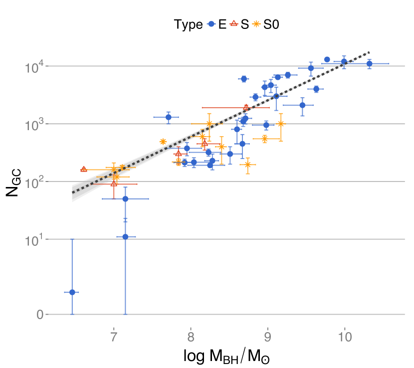
Figure 1: Total number of globular clusters, $N_{\mathrm{GC}}$, plotted versus the central black hole mass, $M_{\mathrm{BH}}$. The dashed line represents the expected value of $N_{\mathrm{GC}}$ for each value of $M_{\mathrm{BH}}$ using Poisson GLM regression, while the shaded areas depicts 50%, 95%, and 99% prediction intervals. Galaxy types are coded by shape and colour as follows: Ellipticals (E; blue solid circles), spirals (S; red open triangles), and lenticulars (S0; orange asterisks). An ArcSinh transformation is applied in the y-axis for better visualization of the whole range of $N_{\mathrm{GC}}$ values, including the null ones.

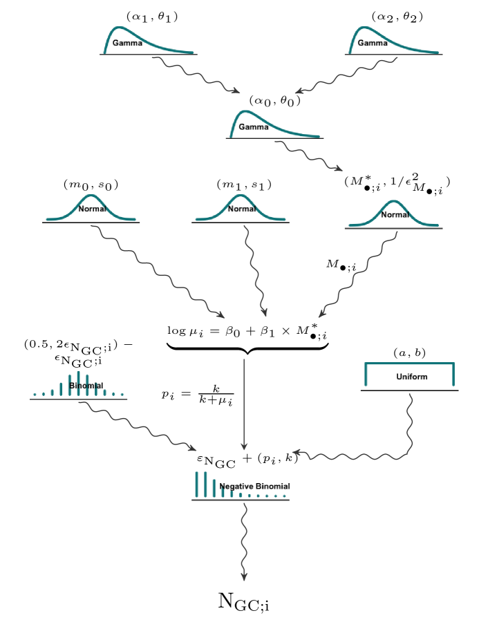
Figure 2: A graphical model of equation (5) representing the hierarchy of dependencies for a data set of galaxies indexed by the subscript $i$. The sinusoidal curves represent stochastic dependencies, while straight arrows a deterministic ones. To save space, we replace $M_{\mathrm{BH}}$ by $M_{\bullet}$ in the diagram.

Within this section we demonstrate the application of Bayesian GLM regression for modelling the relationship between $N_{\mathrm{GC}}$ and the following galaxy properties: $M_{\mathrm{BH}}$, $\sigma$, $M_{V}$ and $M_{\rm dyn}$. Hereafter, unless otherwise stated, the analysis is made using a sub-sample of 45 objects from which we have observations for all the property predictors. In section 5.4 an additional analysis uses the entirety of the available data.

A few common terms in statistical modelling need to be reviewed to facilitate our model applications. The analysis focus is the prediction of $N_{\mathrm{GC}}$ as a function of the global galaxy properties. Therefore, $N_{\mathrm{GC}}$ represents the count (i.e., a non-negative integer) response variable, while $M_{V}$, $M_{\mathrm{BH}}$ and $M_{\rm dyn}$ are interchangeably called covariates, explanatory variables or predictors. If included in the model, the galaxy morphological type is also considered a nominal categorical predictor (see section 3). The whole analysis is performed using JAGS (Just Another Gibbs Sampler), a program for analysis of Bayesian hierarchical models using a Markov Chain Monte Carlo (MCMC) framework. For each regression case, we initiate three Markov chains by starting the Gibbs samples at different initial values sampled from a normal distribution with zero mean and standard deviation of 10. The initial adapting and burning phases were set to 22,000 steps followed subsequently by 50,000 steps, which was sufficient to guarantee convergence of each chain for all studied cases.

We now use the relationship between $M_{\mathrm{BH}}$ and $N_{\mathrm{GC}}$ as an example to illustrate how the statistical model is built. To motivate the use of the more general NB distribution, we start the analysis assuming a GLM Poisson regression model neglecting the uncertainties in measurements at this stage for simplicity. This leads to the following model:

$$N_{\mathrm{GC};i}\sim\rm Poisson(\mu_{i});$$

$$\mu_{i}=e^{\eta_{i}};$$

$$\eta_{i}=\beta_{0}+\beta_{1}\times M_{\mathrm{BH};i};$$ (9)

$$\beta_{0}\sim N(0,10^{6});$$

$$\beta_{1}\sim N(0,10^{6});$$

$$i=1,\cdots,N.$$

This set of equations reads as follows: each galaxy in the dataset, composed of $N$ objects, has its globular cluster population sampled from a Poisson distribution whose expected value, $\mu$, relates to the central black hole mass through a linear relation expressed by $\eta$. Since we don’t have previous information about the values of the coefficients $\beta_{0}$ and $\beta_{1}$, we assigned non-informative Gaussian priors with zero mean and standard deviation equal to $10^{6}$. We refer the reader to appendix A for an example of how to implement a Poisson GLM in JAGS. The fitted curve for this model is displayed in Fig. 1. The grey shaded areas represent 50%, 95%, and 99% prediction intervals, which are the regions where a future observation will fall with these given probabilities. Note that the areas in the plot are too narrow to be visually discriminated. A visual inspection clearly indicates that the Poisson model isn’t adequate to explain the data variability since most of the data fall outside the three prediction intervals. Also, the dispersion statistic for this model is $\mathcal{D}=1039$, which is a strong indication of an inadequate model. All other covariates, $\sigma$, and $M_{V}$ and $M_{\rm dyn}$, lead to models with similarly high levels of Poisson overdispersion. Hence, hereafter we discuss construction of the full model based on the NB family to mitigate overdispersion and to include the uncertainties in the observational quantities. Unlike the Poisson model, by employing a NB distribution we allow the incidence rate of globular clusters to be itself a random variable.

Continuing with our working example, we keep the discussion using the relationship between $N_{\mathrm{GC}}$ and $M_{\mathrm{BH}}$, but see appendix B for descriptions of the other models. The first step is to understand how to include information about the uncertainties in the measurements (see e.g., Andreon & Hurn, 2013, for a review of measurement errors in astronomy). Measurement errors in the response count variable are the trickiest part to be modelled. The classical model with an additive error term $y=y^{*}\pm\varepsilon$ is inappropriate since it does not ensure that the observed value $y$ is non-negative. The appropriate model is described below and its graphical representations are displayed in Fig. 2:

$$N_{\mathrm{GC};i}\sim\rm NB(p_{i},k);$$

$$p_{i}=\frac{k}{k+\mu_{i}};$$

$$\mu_{i}=e^{\eta_{i}}+\epsilon_{N_{GC};i};$$

$$\eta_{i}=\beta_{0}+\beta_{1}\times M_{\mathrm{BH};i}^{*};$$

$$k\sim\mathcal{U}(0,5);$$

$$M_{\mathrm{BH};i}\sim\mathcal{N}(M_{\mathrm{BH};i}^{*},e_{\mathrm{BH};i}^{2});$$

$$\epsilon_{N_{\mathrm{GC}};i}\sim\mathcal{B}(0.5,2e_{N_{GC};i})-e_{N_{\mathrm{GC}};i};$$ (10)

$$\beta_{0}\sim\mathcal{N}(0,10^{6});$$

$$\beta_{1}\sim\mathcal{N}(0,10^{6});$$

$$M_{\mathrm{BH};i}^{*}\sim\Gamma(\alpha_{0},\theta_{0});$$

$$\alpha_{0}\sim\Gamma(0.01,0.01);$$

$$\theta_{0}\sim\Gamma(0.01,0.01);$$

$$i=1,\cdots,N.$$

The above is slightly more complex than the model displayed in equation (5) and reads as follows. Each galaxy in the dataset with $N$ objects, has its globular cluster population sampled from a NB distribution whose expected value, $\mu$, relates to the central black hole mass through the linear predictor $\eta$. The additional transformation $p_{i}=k/(k+\mu_{i})$ is required due to how the NB distribution is parametrized in JAGS. The uncertainties related to the counts, $\epsilon_{N_{\mathrm{GC}};i}$, are taken to be associated with the mean, $\mu$, of the NB distribution and are modelled using a shifted binomial distribution, $\mathcal{B}$, with zero mean and taking on integer values in the range $[-e_{N_{GC};i},+e_{N_{GC};i}]$ (see e.g., Chapter 13 from Cameron & Trivedi, 2013, from which this approach is loosely based.). Uncertainties associated with the observed predictor $M_{BH;i}$ are modelled using a Gaussian distribution with unobserved mean given by the “true black hole mass”, $M_{BH;i}^{*}$, and standard deviations given by the reported uncertainties in the observed black hole mass, $e_{M_{BH};i}$. Since $M_{BH;i}^{*}$ is itself an unobserved variable, we add a non-informative $\Gamma$ prior on top of which we added non-informative hyperpriors for the shape, $\alpha_{0}$, and rate, $\theta_{0}$, parameters of the $\Gamma$ distribution. The choice of a $\Gamma$ prior is motivated by the fact that the black hole mass is a continuous, but non-negative quantity which makes $\Gamma$ a more suitable distribution. For the shape parameter $k$, we assigned a non-informative uniform prior, $\mathcal{U}$, as suggested in Zuur et al. (2013). For the coefficients $\beta_{0}$ and $\beta_{1}$ we assigned non-informative Gaussian priors with zero mean and standard deviation equal to $10^{6}$.

Adapting the model above for each combination of $N_{\mathrm{GC}}$ and a given galaxy property generates the fitted curves displayed in Fig. 3. The grey shaded area represents 50%, 95%, and 99% prediction intervals, while the dashed line represents the expected value of $N_{\mathrm{GC}}$ for each value of the covariate. Note the remarkable agreement between the model and the observed values with prediction intervals enclosing the entirety of the data, including objects that have been previously declared outliers and even removed from analysis, such as our own Milky Way (e.g., Burkert & Tremaine, 2010; Harris & Harris, 2011; Harris et al., 2014).

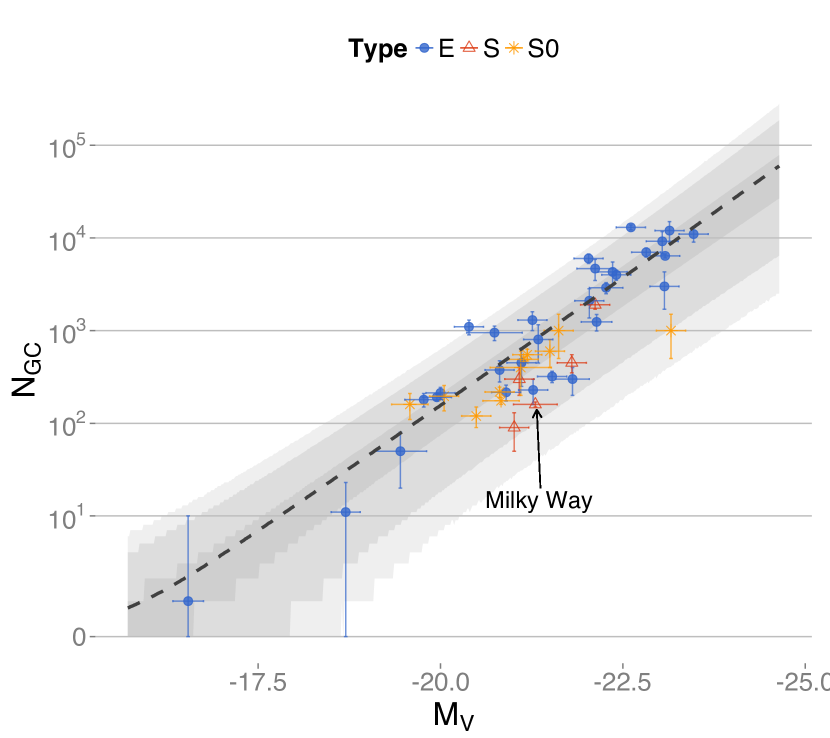
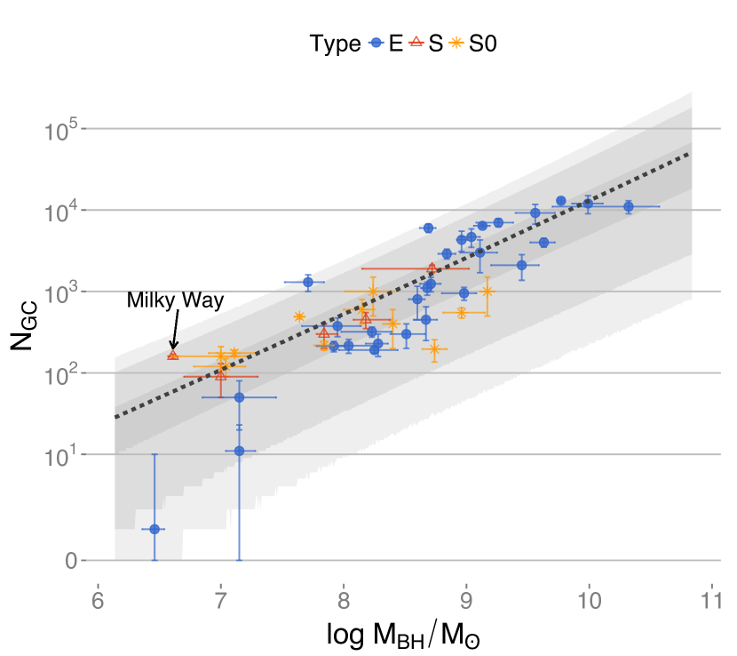
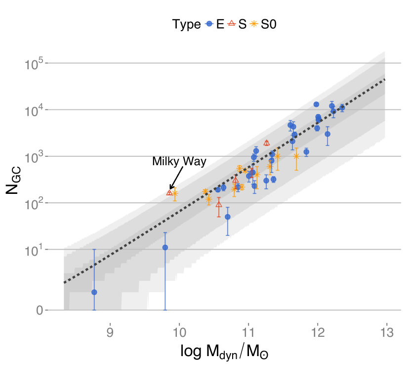
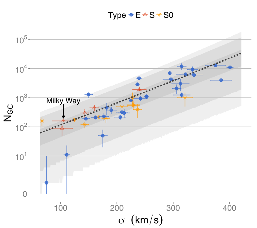
Figure 3: Globular cluster population, $N_{\mathrm{GC}}$ plotted against visual absolute magnitude ($M_{V}$; top left panel), black hole mass ($M_{\mathrm{BH}}$; top right panel), dynamical mass ($M_{\rm dyn}$; bottom left panel), and bulge velocity dispersion ($\sigma$; bottom right panel). In each panel the dashed line represents the expected value of $N_{\mathrm{GC}}$ for each value of the covariate using negative binomial GLM regression, while the shaded areas depicts 50%, 95% , and 99% prediction intervals. Galaxy types are coded by shape and colour as follows: Ellipticals (E; blue solid circles), spirals (S; red open triangles), and lenticulars (S0; orange asterisks). An ArcSinh transformation is applied in the y-axis for better visualization of the whole range of $N_{\mathrm{GC}}$ values, including the null ones.

5.1 Fit diagnostics

If the Markov chains are all representative of the posterior distribution of the fitted parameters, they should overlap each other. Traceplots, Fig. 4, and density plots, Fig. 5 are two useful visual diagnostics that are commonly used to test for chain convergence. We can see that the chains do mix well after the burn-in period, suggesting that the chains are producing representative values from the posterior distribution for $\beta_{0}$, $\beta_{1}$ and $k$. Additionally, we used a more quantitative check, viz., the so-called Gelman-Rubin statistic (Gelman & Rubin, 1992). The underlying idea is that if the chains have reached convergence, the average difference between the chains should be similar to the average difference across steps within the chains. The statistic equals unity if the chains are fully converged. As a rule, values above 1.1 indicate that the chains have failed to properly converge. The Gelman-Rubin statistic fell below 1.05 for all estimated parameters in our analysis. Hence, once we convince ourselves that the model is working properly, the next step in the analysis is to add interpretations to the fitted coefficients as we discuss now.

5.2 Interpretation of the coefficients

The exponentiated coefficients $e^{\beta_{i}}$ of Poisson and NB regressions are also known as rate ratios, or incidence rate ratios, which quantify how an increase of unity in the predictor variable affects the number of occurrences of the response variable. From Table 3, displaying the means and respective 95% credible intervals of the posterior distribution for each parameter, the exponentiated coefficient $\beta_{1}=1.59$ of the $M_{\mathrm{BH}}$ predictor gives a rate ratio of $e^{1.59}=4.9$. Therefore, according to the model, a galaxy whose central black hole has a mass of, e.g., $\approx 10^{8}M_{\bigodot}$ has on average approximately five times more globular clusters than a galaxy whose $M_{\mathrm{BH}}\approx 10^{7}M_{\bigodot}$. In other words, one dex variation increase in the $M_{\mathrm{BH}}$ leads to an approximately five times increase in the incidence of globular clusters in a given galaxy. Likewise, an increase of one dex in $M_{dyn}$ leads to an increase of $e^{2.19}=8.9$ times in the population size of globular clusters. Another way to state this is, given two galaxies with a difference in dynamical mass of one dex, the more massive one has a production rate of globular clusters 8.9 times more efficient on average. Similar interpretation can be made on the other parameters. Another question of interest is how to determine the best predictor of $N_{\mathrm{GC}}$. In the following, we discuss how to address this problem from a Bayesian perspective.

Table 3: $\beta_{i}$ coefficients and scale parameter, $k$, from Bayesian negative binomial regression analysis with $N_{\mathrm{GC}}$ as the response variable and $M_{\mathrm{BH}}$, $M_{\rm dyn}$, $\sigma$ and $M_{V}$ as predictors. The upper and lower limits encloses 95% of the credible intervals around the posterior means.

Predictor	$\beta_{0}$	$\beta_{1}$	k
$M_{\mathrm{BH}}$	$-6.49\pm 2.6$	$1.59\pm 0.30$	$1.53\pm 0.60$
$M_{\rm dyn}$	$-17.72\pm 2.75$	$2.19\pm 0.24$	$2.46\pm 0.97$
$\sigma$	$2.99\pm 0.78$	$0.02\pm 0.003$	$1.52\pm 0.59$
$M_{V}$	$-20.50\pm 3.9$	$-1.28\pm 0.17$	$2.23\pm 1.1$

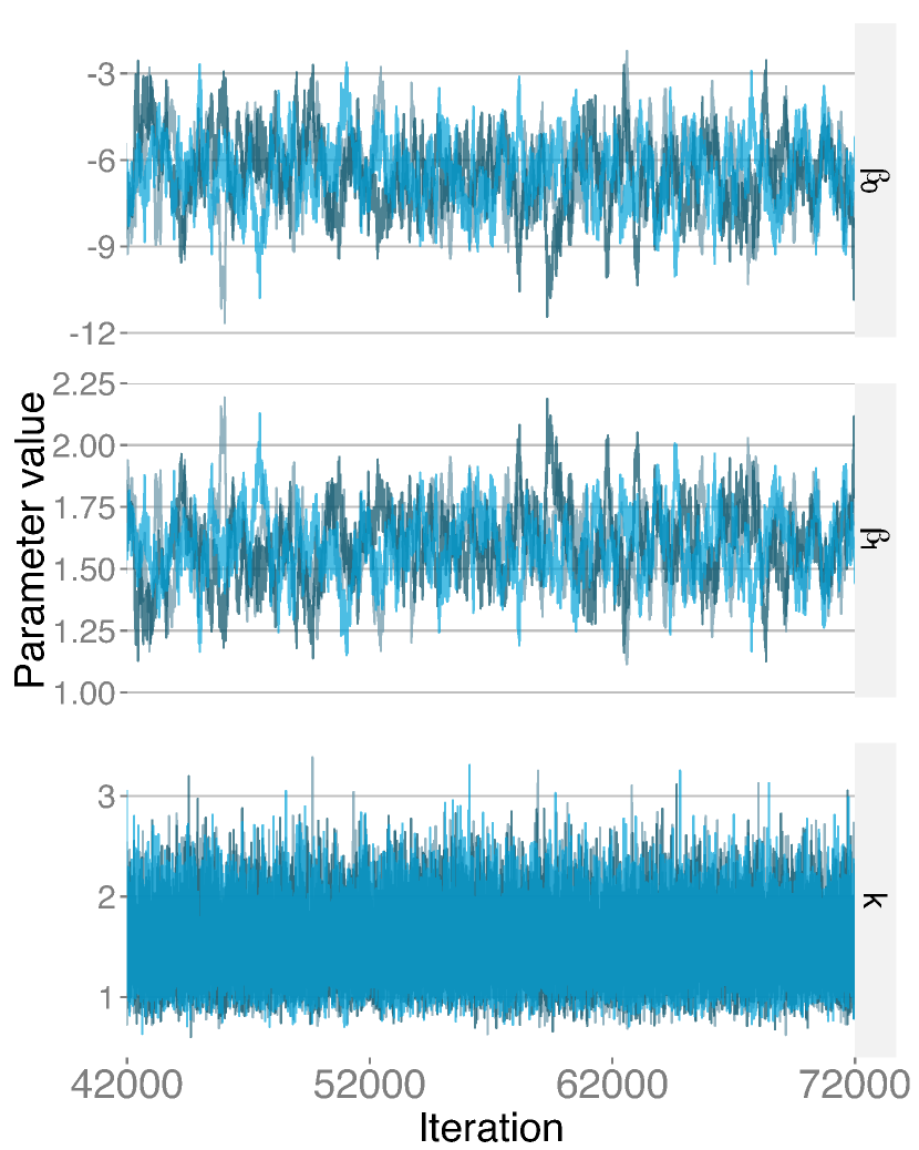
Figure 4: Illustration of MCMC diagnostics. Three chains were generated by starting the Gibbs algorithm at different initial values sampled from a normal distribution with zero mean and standard deviation 10. Steps 42,000-72,000 are shown here. The figure displays the results for the model $N_{\mathrm{GC}}$ vs $M_{\rm BH}$, with the traceplots for $\beta_{0}$, $\beta_{1}$ and $k$ displayed from top to bottom.

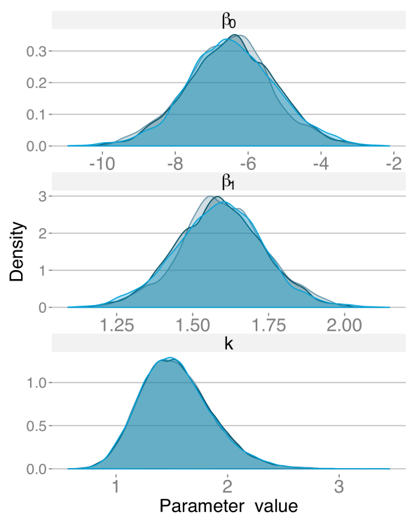
Figure 5: Overlapped density plots with different colors by chain. The plot is a comparison of the target distribution by each chain, representing a visual test for convergence. The figure displays the results for the model $N_{\mathrm{GC}}$ vs $M_{\rm BH}$, with the posteriors for $\beta_{0}$, $\beta_{1}$ and $k$ displayed from top to bottom.

5.3 Model Comparison

To find the best predictors for the globular cluster population, we compare the models using the dispersion statistics $\mathcal{D}$ defined in section 3.2, and the deviance information criterion (DIC; Spiegelhalter et al., 2002). The latter represents a compromise between the goodness of fit and model complexity. It is defined as:

$$DIC=\overline{Dev}+p_{D},$$ (11)

where the $\overline{Dev}$ is the average of the deviance $Dev(\mathbf{\theta})$ defined as $Dev(\mathbf{\theta})=-2\log\mathcal{L}(\rm{data}|\mathbf{\theta})$, with $\mathcal{L}$ representing the likelihood function. The effective number of parameters, $p_{D}$, is calculated as:

$$p_{D}=\overline{Dev}-Dev(\mathbf{\theta}),$$ (12)

where $\mathbf{\theta}$ is the vector of model parameters (${\beta_{0},\beta_{1},k}$ for the case in study here). The preferred model has the smallest value for the DIC statistic. Figs. 6 and 7 depict the results for the model comparison using the same dataset. The black hole mass displays the lowest values for $\mathcal{D}$ and DIC, with dispersion statistics as low as $\mathcal{D}=1.05$. Although derived from an independent analysis, these findings corroborate previous claims about the tight connection between the central black hole mass and globular cluster population (Burkert & Tremaine, 2010). Nevertheless, it’s worth noting that this is not in agreement with a previous analysis performed by Harris et al. (2013) using the same catalogue, where they found $M_{\rm dyn}$ as a better predictor for $N_{\mathrm{GC}}$ than $M_{\rm BH}$.

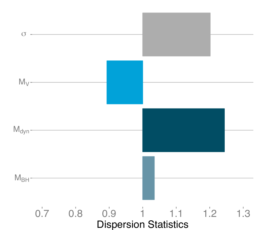
Figure 6: Dispersion statistics, $\mathcal{D}$, for each model. Values above 1 represent overdispersion, while values below 1 indicate underdispersion.

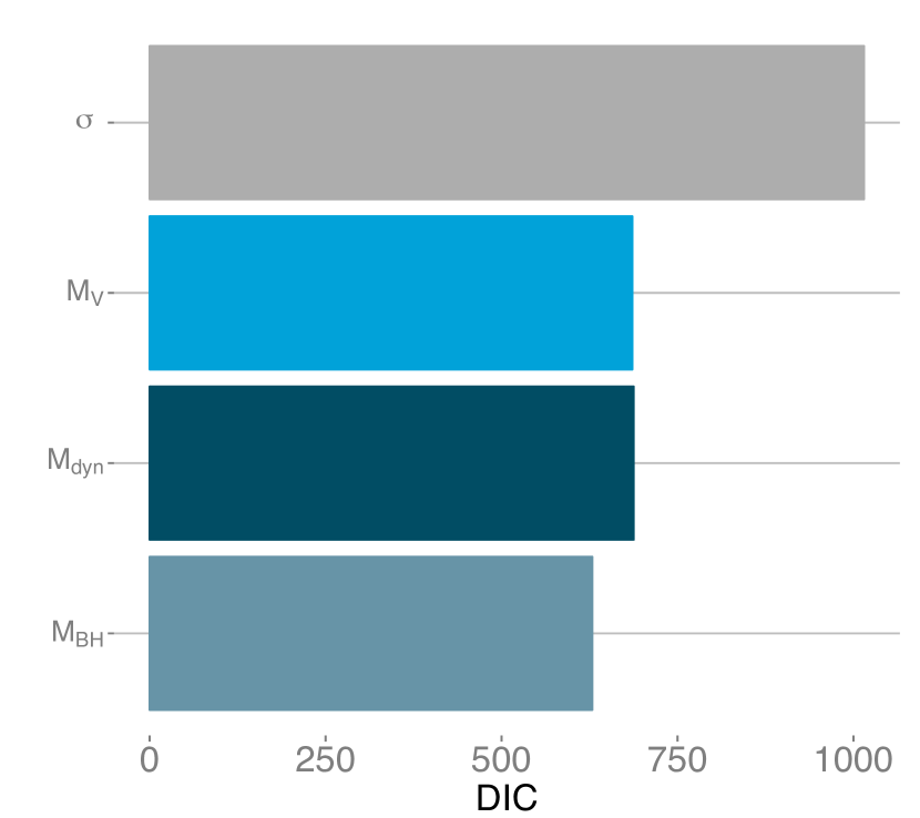
Figure 7: Deviance information criterion, DIC, for each model. Smaller DIC values correspond to preferred models.

5.4 Further analysis with the entire data set

Hereafter, we provide a more extensive analysis using the entire catalogue of 422 galaxies. The only quantities available for all objects are the $N_{\mathrm{GC}}$, galaxy morphological type and $M_{V}$ (Harris et al., 2013). The advantage of using count models for this type of analysis is apparent from the six galaxies for which no globular clusters were detected. Such a scenario is naturally accommodated by discrete likelihoods while avoiding the failings of logarithmic transformations to the response. The statistical model we use is the same as that discussed in the beginning of this section and can be described as:

$$N_{\mathrm{GC};i}\sim\rm NB(p_{i},k);$$

$$p_{i}=\frac{k}{k+\mu_{i}};$$

$$\mu_{i}=e^{\eta_{i}}+\epsilon_{N_{GC};i};$$

$$\eta_{i}=\beta_{0}+\beta_{1}\times M_{V;i}^{*};$$

$$k\sim\mathcal{U}(0,5);$$

$$M_{V;i}\sim\mathcal{N}(M_{V;i}^{*},e_{M_{V};i}^{2});$$

$$\epsilon_{N_{GC};i}\sim\mathcal{B}(0.5,2e_{N_{GC};i})-e_{N_{GC};i};$$ (13)

$$\beta_{0}\sim\mathcal{N}(0,10^{6});$$

$$\beta_{1}\sim\mathcal{N}(0,10^{6});$$

$$M_{V;i}^{*}\sim\mathcal{U}(-26,-10);$$

$$i=1,\cdots,N.$$

Overall, the model is similar to the one described in equation (5). The difference is in the prior for the unobserved true absolute visual magnitude, $M_{V;i}^{*}$, to which we assigned a uniform prior over the range of magnitudes covered by the catalogue. The fitted model shows remarkable agreement with the data as displayed in Fig. 8. Very few objects fall outside the prediction intervals over a wide range of galaxy brightnesses. The dispersion statistics for this model is $\mathcal{D}=1.15$, and the credible intervals for the fitted $\beta$ coefficients and scaling parameter, $k$, are shown in Fig. 9. Likewise, as in the previous section, we can interpret the $\beta$ coefficient as follows. The mean value of $\beta_{1}$ exponentiated is $\approx 0.4$, which implies that a galaxy whose absolute visual magnitude is one unit greater than another reference galaxy has on average 0.4 times less globular clusters; i.e., a galaxy brighter by one magnitude over another has on average 2.5 times more globular clusters. Likewise, a galaxy with $M_{V}=-20$ has on average $2.5^{5}\approx 100$ times more globular clusters than a galaxy with $M_{V}=-15$, which is consistent with a visual inspection of Fig. 8. Another advantage of our approach is the possibility to extrapolate the regression solution without making non-physical predictions. The fitted model predicts a nearly zero occurrence of globular clusters for galaxies with $M_{V}\geqslant-11$. Considering the total galaxy luminosity, $L=10^{0.4(M_{V_{\bigodot}}-M_{V})}L_{\bigodot}$, with $M_{V_{\bigodot}}=4.83$, the model suggests that galaxies with $L\leqslant 2\times 10^{6}~{}L_{\bigodot}$ are unlikely to host populations of globular clusters, thus agreeing with the literature (e.g., Harris et al., 2013). The use of Bayesian prediction intervals allow us to make some interesting predictions: for instance from Fig. 8, we can state that galaxies with luminosities $L\leqslant 8.5\times 10^{7}~{}L_{\bigodot}$ (or $M_{V_{\bigodot}}\geqslant-15$) should not contain more than 10 globular clusters with 99% probability.

The analysis performed so far did not account for information regarding different galaxy morphological types. Therefore, we are implicitly assuming a pooled estimate (e.g., Gelman & Hill, 2007): all different galaxy types are sampled from the same common distribution ignoring any possible variation among them. On the other extreme, performing an independent analysis for each class would mean making the assumption that each morphological type is sampled from independent distributions and that variations between them cannot be combined. In the next section we discuss a more flexible approach together with a brief overview of generalized linear mixed models.

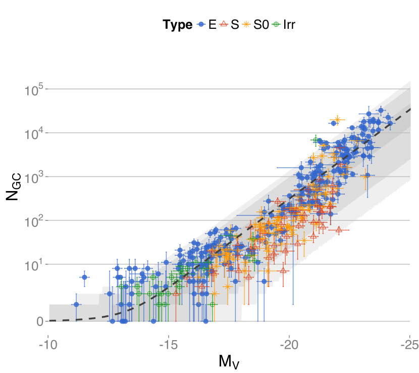
Figure 8: Globular cluster population, $N_{\rm GC}$ plotted against visual absolute magnitude $M_{V}$. The dashed line represents the expected value of $N_{\mathrm{GC}}$ for each value of $M_{V}$, while the shaded areas depicts 50%, 95%, and 99% prediction intervals. Galaxy types are coded by shape and colour as follows: Ellipticals (E; blue solid circles), spirals (S; red open triangles), lenticulars (S0; orange asterisks), and irregulars (Irr; green open circles). An ArcSinh transformation is applied in the y-axis for better visualization of the whole range of $N_{\rm GC}$ values, including the null ones.

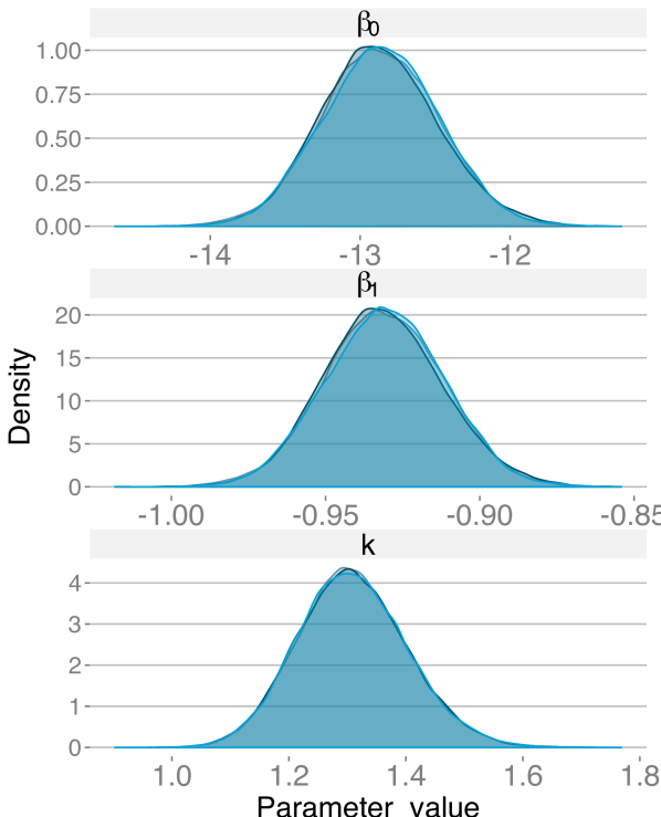
Figure 9: Overlapped density plots with different colors by chain. The plot is a comparison of the target distribution by each chain, representing a visual test for convergence. The figure displays the results for the model $N_{\rm GC}$ vs $M_{V}$, with the posteriors for $\beta_{0}$, $\beta_{1}$ and $k$ displayed from top to bottom.

6 Generalized Linear Mixed Models

As our final analysis, we introduce one of the most important extensions of the GLM methodology known as generalized linear mixed models (GLMMs). In particular, we focus on one of the simplest GLMM incarnations known as the random intercepts model. The random intercepts model, in our context, includes an additional term $\zeta_{j}$ to account for a class (galaxy type) specific deviation from the common intercept $\beta_{0}$:

$$\eta_{ij}=\beta_{0}+\beta_{1}\times M_{V;i}+\zeta_{j},$$ (14)

where the index $j$ runs from 1 to 69 representing each of the different galaxy subtypes reported in Harris et al.. A standard approach to modelling $\zeta_{j}$ in a standard linear mixed regression model is to assume the conditional normality of the random intercepts with $\zeta_{j}\sim\mathcal{N}(0,1/\tau)$, and $\tau\sim\Gamma(0.01,0.01)$. Our intention in incorporating this extra term into the model is not to simply adjust the data, but rather the aim is to identify any particular galaxy sub-type which deviates from the overall population mean. For this purpose, we employed a popular method for variable selection from a Bayesian perspective known as least absolute shrinkage and selection operator (LASSO) which is discussed in the following section.

6.1 Bayesian LASSO

The original LASSO regression was proposed by Tibshirani (1996) to automatically select a relevant subset of predictors in a regression problem by shrinking some coefficients towards zero (see also Uemura et al., 2015, for a recent application of LASSO for modelling Type Ia supernovae light curves). For a typical linear regression problem:

$$y_{i}=\beta_{0}+\beta_{1}x_{1}+\cdots+\beta_{p}x_{p}+\epsilon,$$ (15)

with $\epsilon$ denoting Gaussian noise, LASSO estimates linear regression coefficients $\mathbf{\beta}=\beta_{0}+\beta_{1}x_{1}+\cdots+\beta_{p}x_{p}$ by imposing a $L_{1}$-norm penalty in the form:

$$\arg\!\min_{\beta}\left\{\sum_{i=1}^{N}\left(y_{i}-\sum_{j=1}^{p}\beta_{j}x_{ij}\right)^{2}+\kappa\sum_{j=1}^{p}|\beta_{j}|\right\},$$ (16)

where $\kappa\geq 0$ is a tunable constant that controls the level of sparseness of the solution. The number of zero coefficients thereby increases as $\kappa$ increase. Tibshirani also noted that the LASSO estimate has a Bayesian counterpart when the $\mathbf{\beta}$ coefficients have a double-exponential prior (i.e., a Laplace prior) distribution,

$$f(\mathbf{\zeta};\tau)=\frac{1}{2\tau}\exp\left(-\frac{|\zeta_{j}|}{\tau}\right),$$ (17)

where $\tau=1/\kappa$. The idea was further developed and is known as Bayesian LASSO (see e.g., Park et al., 2008). Hereafter, we use the LASSO formulation for a slightly different purpose, viz., variable selection for random intercept models (see e.g., Bernardo et al., 2011, pg. 165). The underlying idea is to discriminate between galaxy types that follow the overall population mean, i.e. $\zeta_{1}=0$, and galaxies that require an additional adjustment in the intercept, i.e. $\zeta_{i}\neq 0$. In order to include this information, we replace the linear predictor $\eta$ by equation (14) and add the following equations in the model described by equation (5.4):

$$\zeta_{j}\sim Laplace\left(0,\tau\right);$$

$$\tau=1/\kappa;$$ (18)

$$\kappa\sim\Gamma(0.01,0.01);$$

$$j=1,\cdots,69.$$

The role of the Laplace prior is to assign more weight to regions either near to zero or in the distribution tails as compared to a normal prior. A visual inspection on Fig. 10 confirms this notion. For the parameter $\kappa$, we assigned a diffuse (non-informative) gamma hyperprior in the form $\kappa\sim\Gamma(0.01,0.01)$, which avoids the need of an ad hoc choice of $\kappa$. Note that other possibilities exist such as, e.g., iteratively finding $\kappa$ via cross-validation to maximize predictive power.

Analysis results are displayed on Fig. 11. Overall, it suggests that we do not need to add an additional intercept for predicting $N_{\mathrm{GC}}$ from $M_{V}$. This is consistent with the fact that prediction intervals in Fig. 8 enclose $\sim 98.8\%$ of the data set without any need of a random intercept. Nevertheless, the following galaxy types require systematic adjustments: spirals galaxies with moderate size of nuclear bulge (Sb), barred lenticulars (SB0), lenticulars (S0) and dwarf elliptical galaxies (dE0N and dE1N). MG represents one single object. Also, UGC 3274 is the brightest galaxy of the galaxy cluster ACO 539 (Lin & Mohr, 2004). Fig. 12 shows that the dE0N and dE1N objects have a large number of GCs on average when compared to other galaxy types with similar luminosities, while the lenticulars have systematically fewer GCs than expected for the overall galaxy population. This can be quantified by looking at the mean value of $\zeta$ in Fig. 11. For S0 galaxies the mean value of $\zeta$ is -0.42 indicating that, on average, S0 galaxies have 34% ($1-e^{-0.42}$) fewer GCs than other galaxy types in the same range of luminosities. Generally speaking, galaxy types with 95% credible intervals falling on the right side of the dashed grey vertical line in Fig. 11 have more GCs than the overall population mean, while galaxy types on the left side have fewer GCs than the population mean. While a detailed investigation of the causes of this behaviour is beyond the scope of this work, it is important to stress the ability of hierarchical Bayesian models to explore the multilevel statistical properties of the objects under study in an unified way.

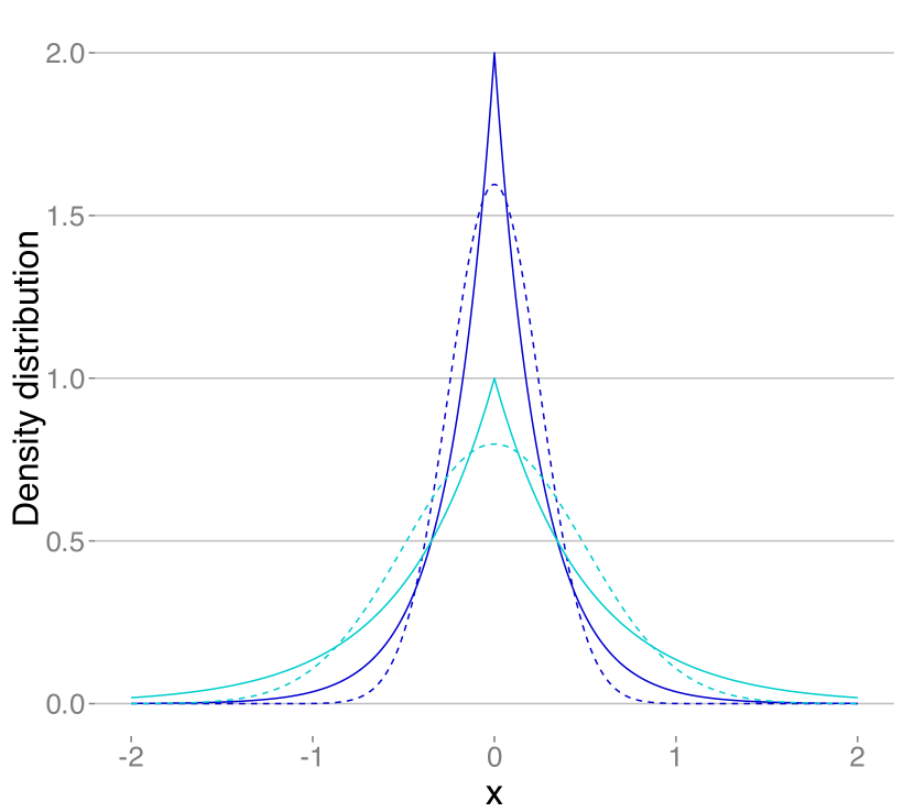
Figure 10: Illustrative comparison between Laplace and Gaussian priors. The Gaussian distribution is represented by dashed lines, while the Laplace distribution by solid lines. For all curves we assign a zero mean, and the scale (or standard deviation, $\sigma$, for the Gaussian case) parameters 0.25 (dark blue lines) and 0.5 (cyan lines).

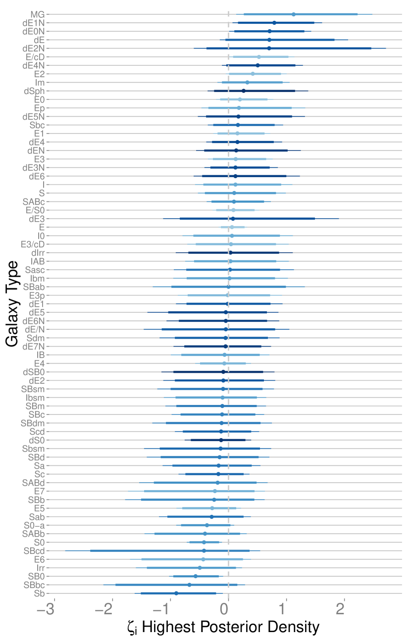
Figure 11: Caterpillar plot for the random intercepts $\zeta_{i}$ versus the subcategories of galaxy morphological classifications. The thick and thin horizontal lines represent 90% and 95% credible intervals respectively.

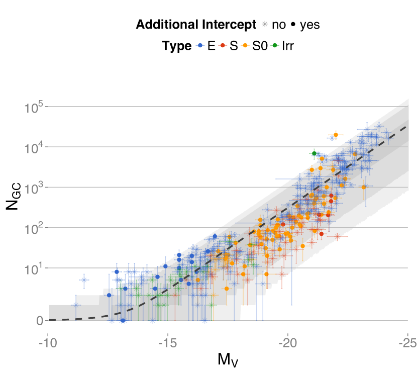
Figure 12: Globular cluster population, $N_{\mathrm{GC}}$ plotted against visual absolute magnitude $M_{V}$. The dashed line represents the expected value of $N_{\mathrm{GC}}$ for each value of $M_{V}$, while the shaded areas depicts 50%, 95%, and 99% prediction intervals. Galaxy types are coded by colours as follows: Ellipticals (E; blue), spirals (S; red), lenticulars (S0; orange), and irregulars (Irr; green). Asterisks represent galaxies belonging to sub-types whose random intercept $\zeta$ is consistent with zero, while circles represent the ones with $\zeta\neq 0$. An ArcSinh transformation is applied in the y-axis for better visualization of the whole range of $N_{\mathrm{GC}}$ values, including the null ones.

7 Conclusions

We employed a Bayesian negative binomial regression model to analyse the population size of globular clusters in the presence of galactic attributes such as central black hole mass, brightness, and morphological type. Hence, demonstrating how generalized linear models designed to represent count data provide reliable outcomes and interpretations. The main scientific results and features of our analysis can be summarized as follows:

• The population size of GC is on average 35% lower on S0 galaxies if compared to other galaxies with similar luminosities.

• The relationship between the number of globular clusters and other galaxy properties has more variation than expected by a Poisson process, but can be well modelled by a negative binomial GLM.

• The Bayesian modelling herein employed naturally accounts for heteroscedasticity, intrinsic scatter, and errors in measurements in both axes (either discrete or continuous).

• Predicted intervals around the trend for expected $N_{\mathrm{GC}}$ envelope the data, including the Milky Way, which was previously considered an outlier.

• The random intercepts model (with a Bayesian LASSO) applied to the correlation between GC population and brightness allow us to account for the presence of 69 different galaxy subcategories of morphological classifications, and automatically identifies particular types not following the overall population mean. Galaxy types dE1N, dE0N, E/cD, S0, Sb0 and Sb show significant deviations from the general trend. Based on the sample studied here, we advise these types to be further scrutinized in order to clarify if there is any physical mechanism behind such deviations or merely an observational bias.

• By employing a hierarchical Bayesian model for the random intercepts and unobserved covariates (e.g., true black hole mass), we allow the model to borrow strength across units. This happens via their joint influence on the posterior estimates of the unknown hyper-parameters.

• If extrapolated, the fitted model predicts a suppression in the presence of GCs for galaxies with luminosities $L\lesssim 2\times 10^{6}~{}L_{\bigodot}$.

• The central black holes mass is in fact a good predictor of the number of GCs. One dex increase in $M_{BH}$ leads to an approximate 5 times increase in the incidence of globular clusters. The origin of such correlation it is still a matter of debate. One possible explanation is that both properties are associated with a common event such as major mergers, thus galaxies experimenting a recent major merger should have a large $M_{BH}$ mass and GC populations (e.g., Jahnke & Macciò, 2011). The total mass of GCs and the central black hole mass can also correlate with the bulge binding energy in elliptical galaxies (e.g., Snyder et al., 2011; Saxton et al., 2014). Rapid growth of the nuclear black hole of a galaxy might be fuelled by a massive inflow of cold gas towards the centre of the galaxy. The gas inflow would trigger star formation and the formation of GCs. Hence, leading to an indirect correlation between the total number of GCs and the $M_{BH}$. Scrutinizing which one among these and other possibilities, if any, are responsible for this correlation (causal or not) is beyond the purposes of this work. However, it does provide a clear example on how the adoption of modern statistical methods can point to intriguing astrophysical questions.

A statistical model is based on an appropriate probability distribution function assumed to generate or describe a data set. Hence, the parameter estimating likelihood function must specify a probability distribution on the appropriate scale under study. Discrete data, and count data in particular, are not continuous as are data described by the Gaussian distribution. The most appropriate way to model count data is by using a discrete probability distribution, e.g., a Poisson or negative binomial likelihood, otherwise the model will likely be biased and misspecified — the price to be paid for employing the wrong likelihood estimator for the data of interest.

Generalized linear models are a cornerstone of modern statistics, and an invaluable instrument for astronomical investigations given their potential application to a variety of astronomical problems beyond Gaussian assumptions. A prompt integration of these methods into astronomical analyses will allow contemporary statistical techniques to become common practice in the research of $\rm 21^{st}$ century astronomy.

Appendix A JAGS model

Poisson GLM

The basic JAGS syntax for a Poisson GLM model:

⬇

1GLM.pois<-model{

2#Priors for regression coefficients

3

4beta.0~dnorm(0,0.000001)

5beta.1~dnorm(0,0.000001)

6

7#Poisson GLM Likelihood

8

9for (i in 1:N){

10eta[i]<-beta.0+beta.1*x[i]

11log(mu[i])<-eta[i]

12y[i]~dpois(mu[i])

13 }

14}

Negative Binomial GLM

The basic JAGS syntax for a NB GLM model:

⬇

1GLM.NB<-model{

2#Priors for regression coefficients

3

4beta.0~dnorm(0,0.000001)

5beta.1~dnorm(0,0.000001)

6k~dunif(0.001,10)

7

8#NB GLM Likelihood

9

10for (i in 1:N){

11eta[i]<-beta.0+beta.1*x[i]

12log(mu[i])<-eta[i]

13p[i]<-k/(k+mu[i])

14y[i]~dnegbin(p[i],k)

15 }

16}

Another approach to fit a NB model in JAGS is via a combination of a Gamma distribution with a Poisson distribution in the form (see e.g., Marley & Wand, 2010; Hilbe, 2011):

⬇

1GLM.NB<-model{

2#Priors for regression coefficients

3

4beta.0~dnorm(0,0.000001)

5beta.1~dnorm(0,0.000001)

6k~dunif(0.001,10)

7

8#NB GLM Likelihood

9

10for (i in 1:N){

11eta[i]<-beta.0+beta.1*x[i]

12log(mu[i])<-eta[i]

13rateParm[i]<-k/mu[i]

14g[i]~dgamma(k,rateParm[i])

15y[i]~dpois(g[i],k)

16 }

17}

Appendix B Bayesian model for each covariate

Dynamical mass versus globular cluster population

Bayesian NB GLM model for the relationship between $N_{\mathrm{GC}}$ and galaxy dynamical mass $M_{dyn}$. Since, there is no information about the uncertainties in the measurements of $M_{dyn}$, we neglect this in this particular model.

$$N_{GC;i}\sim\rm NB(p_{i},k);$$

$$p_{i}=\frac{k}{k+\mu_{i}};$$

$$\mu_{i}=e^{\eta_{i}}+\epsilon_{N_{GC};i};$$

$$\eta_{i}=\beta_{0}+\beta_{1}\times M_{dyn;i};$$

$$k\sim\mathcal{U}(0,5);$$

$$\epsilon_{N_{GC};i}\sim\mathcal{B}(0.5,2e_{N_{GC};i})-e_{N_{GC};i};$$ (19)

$$\beta_{0}\sim\mathcal{N}(0,10^{6});$$

$$\beta_{1}\sim\mathcal{N}(0,10^{6});$$

$$\alpha_{0}\sim\Gamma(0.01,0.01);$$

$$\theta_{0}\sim\Gamma(0.01,0.01);$$

$$i=1,\cdots,N.$$

Bulge velocity versus globular cluster population

Bayesian NB GLM model for the relationship between $N_{\mathrm{GC}}$ and bulge dispersion velocity $\sigma$.

$$N_{GC;i}\sim\rm NB(p_{i},k);$$

$$p_{i}=\frac{k}{k+\mu_{i}};$$

$$\mu_{i}=e^{\eta_{i}}+\epsilon_{N_{GC};i};$$

$$\eta_{i}=\beta_{0}+\beta_{1}\times\sigma_{i}^{*};$$

$$k\sim\mathcal{U}(0,5);$$

$$\sigma_{i}\sim\mathcal{N}(\sigma_{i}^{*},e_{\sigma_{i}}^{2});$$

$$\epsilon_{N_{GC};i}\sim\mathcal{B}(0.5,2e_{N_{GC};i})-e_{N_{GC};i};$$ (20)

$$\beta_{0}\sim\mathcal{N}(0,10^{6});$$

$$\beta_{1}\sim\mathcal{N}(0,10^{6});$$

$$\sigma_{i}^{*}\sim\Gamma(\alpha_{0},\theta_{0});$$

$$\alpha_{0}\sim\Gamma(0.01,0.01);$$

$$\theta_{0}\sim\Gamma(0.01,0.01);$$

$$i=1,\cdots,N.$$

References

- Andreon & Hurn (2013) Andreon S., Hurn M., 2013, Statistical Analysis and Data Mining, 6, 15
- Andreon & Hurn (2010) Andreon S., Hurn M. A., 2010, MNRAS, 404, 1922
- Ata et al. (2015) Ata M., Kitaura F.-S., Müller V., 2015, MNRAS, 446, 4250
- Bernardo et al. (2011) Bernardo J., Bayarri J., Berger J., Dawid A., Heckerman D., 2011, Bayesian Statistics 9. Oxford science publications, OUP Oxford
- Brodie & Strader (2006) Brodie J. P., Strader J., 2006, ARA&A, 44, 193
- Burkert & Tremaine (2010) Burkert A., Tremaine S., 2010, ApJ, 720, 516
- Cameron & Trivedi (2013) Cameron A. C., Trivedi P. K., 2013, Regression analysis of count data, second edition. Cambridge University Press
- De Souza et al. (2015) De Souza R. S., Cameron E., Killedar M., Hilbe J., Vilalta R., Maio U., Biffi V., Ciardi B., Riggs J., 2015, Astronomy and Computing, 12, 21
- Durrell et al. (2014) Durrell P. R., Côté P., Peng E. W., Blakeslee J. P., Ferrarese L., Mihos J. C., Puzia T. H., Lançon A., et al. 2014, ApJ, 794, 103
- Elliott et al. (2015) Elliott J., de Souza R. S., Krone-Martins A., Cameron E., Ishida E. E. O., Hilbe J., 2015, Astronomy and Computing, 10, 61
- Gebhardt et al. (2000) Gebhardt K., Bender R., Bower G., Dressler A., Faber S. M., Filippenko A. V., Green R., Grillmair C., Ho L. C., Kormendy J., Lauer T. R., Magorrian J., Pinkney J., Richstone D., Tremaine S., 2000, ApJ, 539, L13
- Gelman & Hill (2007) Gelman A., Hill J., 2007, Data analysis using regression and multilevel/hierarchical models. Analytical methods for social research, Cambridge University Press, New York
- Gelman & Rubin (1992) Gelman A., Rubin D. B., 1992, Statist. Sci., 7, 457
- Griswold et al. (2004) Griswold M., Parmigiani G., Potosky A., Lipscomb J., 2004, Biostatistics, 1, 1
- Hardin & Hilbe (2012) Hardin J. W., Hilbe J. M., 2012, Generalized Linear Models and Extensions, 3rd edn. StataCorp LP
- Harris & Harris (2011) Harris G. L. H., Harris W. E., 2011, MNRAS, 410, 2347
- Harris et al. (2014) Harris G. L. H., Poole G. B., Harris W. E., 2014, MNRAS, 438, 2117
- Harris et al. (2013) Harris W. E., Harris G. L. H., Alessi M., 2013, ApJ, 772, 82
- Hilbe (2014) Hilbe J., 2014, Modeling Count Data. Cambridge University Press
- Hilbe (2011) Hilbe J. M., 2011, Negative binomial regression, 2nd edn. Cambridge University Press
- Jahnke & Macciò (2011) Jahnke K., Macciò A. V., 2011, ApJ, 734, 92
- Jong & Heller (2008) Jong P. D., Heller G. Z., 2008, Generalized Linear Models for Insurance Data. Cambridge University Press
- Kruijssen (2014) Kruijssen J. M. D., 2014, Classical and Quantum Gravity, 31, 244006
- Lansbury et al. (2014) Lansbury G. B., Lucey J. R., Smith R. J., 2014, MNRAS, 439, 1749
- Lin & Mohr (2004) Lin Y.-T., Mohr J. J., 2004, ApJ, 617, 879
- Lindsey (1999) Lindsey J. K., 1999, Statistics in medicine, 18, 2223
- Marley & Wand (2010) Marley J. K., Wand M. P., 2010, Journal of Statistical Software, 37, 1
- Marschner & Gillett (2012) Marschner I. C., Gillett A. C., 2012, Biostatistics, 13, 179