Blind Stereoscopy of the Coronal Magnetic Field

Abstract

We test the feasibility of 3D coronal-loop tracing in stereoscopic EUV image pairs, with the ultimate goal of enabling efficient 3D reconstruction of the coronal magnetic field that drives flares and coronal mass ejections (CMEs). We developed an automated code designed to perform triangulation of coronal loops in pairs (or triplets) of EUV images recorded from different perspectives. The automated (or blind) stereoscopy code includes three major tasks: (i) automated pattern recognition of coronal loops in EUV images, (ii) automated pairing of corresponding loop patterns from two different aspect angles, and (iii) stereoscopic triangulation of 3D loop coordinates. We perform tests with simulated stereoscopic EUV images and quantify the accuracy of all three procedures. In addition we test the performance of the blind stereoscopy code as a function of the spacecraft-separation angle and as a function of the spatial resolution. We also test the sensitivity to magnetic non-potentiality. The automated code developed here can be used for analysis of existing Solar TErrestrial RElationship Observatory (STEREO) data, but primarily serves for a design study of a future mission with dedicated diagnostics of non-potential magnetic fields. For a pixel size of 0.6^′′(corresponding to the Solar Dynamics Observatory (SDO) Atmospheric Imaging Assembly (AIA) spatial resolution of 1.4^′′), we find an optimum spacecraft-separation angle of $\alpha_{s}\approx 5^{\circ}$.

1 Introduction

One critically needed tool for forecasting severe geomagnetic storms well ahead of time is a reliable method to map the magnetic field erupting into the heliosphere during coronal mass ejections (CMEs) so that its evolution can be modeled well before their field impacts Earth’s (e.g. Schrijver et al., 2015). A major impediment at present is that we cannot reliably describe the magnetic field in nascent CMEs as their erupting structure enters the heliosphere.

Even with recent advances in the ready availability of vector-magnetic data on active regions, the modeling of the configuration of the coronal field above these regions remains a challenge. Model results based on surface observations alone are generally ambiguous and not well representative of the observed coronal configuration (e.g. DeRosa et al., 2009, and references therein). The use of coronal-loop trajectories to guide field models towards a solution compatible with surface-field measurements shows promise (Malanushenko et al., 2012, 2014), but the fact that only the 2D trajectories projected against the plane of the sky are available presents a stumbling block that needs to be overcome. Malanushenko et al., (2012) approximate the third coordinate, along the line-of-sight (LOS), by pairing up each observed coronal loop with the best-fitting field line of a linear force-free field (using separate field lines for each loop), and they then iterate towards a non-linear force-free field while continually nudging the overall solution back to the set of 3D loop trajectories first determined. Whereas this results in a model field that by design matches the observed loops quite well, it is unlikely that the input 3D trajectories are entirely correct (e.g. see differences between 2D and 3D reconstructions in Aschwanden 2013b). Until we have a way to measure the 3D loop trajectories we cannot truly validate the method, but once the 3D trajectories are known, they can of course be used from the outset to guide the model field towards a solution compatible with the observed 3D configuration.

Here, we study a concept with two or three spacecraft that provide stereoscopic views of EUV images of coronal loops, which when combined with photospheric line-of-sight magnetograms, provide information suitable for 3D reconstruction of the coronal magnetic field. One possible orbital spacecraft configuration is formed by the Sun–Earth Lagrangian points L1 and L4 (or L5), similar as it was obtained when the Solar TErrestrial RElationship Observatory (STEREO) A(head) and B(ehind) spacecraft moved near the L4 and L5 points in 2008, while the Solar and Heliospheric Observatory (SOHO) was positioned in L1. However, that was a very temporary configuration, with instrumentation at moderate resolution. Ideally, a new generation of instruments should have a spatial resolution that is comparable to that of Solar Dynamics Observagory (SDO)’s Atmospheric Imaging Assembly (AIA), and a field of view at least as large as supported by its $4k\times 4k$ imaging cameras with 0.6^′′pixels. Unlike the STEREO–SOHO configuration, a scientifically more promising mission should provide a long-lived multi-spacecraft configuration, providing images with essentially identical passband and telescope characteristics.

We envision that a pair (or perhaps a triplet) of spacecraft equipped with the necessary instruments could support the autonomous calculations of the coronal magnetic field, its non-potentiality, and the free energies in each active region either in near-real time or with up to at most a day delay, so that this compound observatory can be used to understand active-region instabilities and heliospheric model input, and as an early-warning system for severe space-weather storms. To succeed, the data-processing and modeling capabilities would require (i) automated pattern recognition of coronal loops in EUV images, (ii) automated stereoscopic pairing of coronal loops, (iii) stereoscopic triangulation of coronal loops, and (iv) nonlinear force-free field forward-fitting that yields the non-potential magnetic field, its free energy, and (v) - after eruptions - quantitative information on the ejecta into the heliosphere. We demonstrate the feasibility of the first four of these automated tasks in this study, and we constrain the optimum configuration for the angular spacecraft separation.

Recent reviews on solar stereoscopy and tomography have been presented by Aschwanden (2011), and recent reviews on the coronal magnetic field are given by Wiegelmann and Sakurai (2012) and Wiegelmann, Thalmann, and Solanki (2014). Early attempts of solar stereoscopy using information from a single spacecraft (using XUV images from Skylab) used the solar rotation to measure stereoscopic parallaxes (Berton and Sakurai 1985), which requires (unrealistic) static coronal loops on time scales of at least one day, but hydrodynamic heating and cooling processes of loops occur on time scales of $\approx 10^{3}$ seconds in active regions (e.g. Warren and Winebarger 2007), even as the field’s photospheric boundary is evolving underneath. A dynamic solar-rotation stereoscopy method was developed later by Aschwanden et al., (1999, 2000), which relieves the requirement of static loops in lieu of a quasi-static magnetic field. This assumption is somewhat more realistic, but breaks down after about one day, since photospheric magnetic fields involved in major flaring and eruptions were observed to have characteristic growth and decay timescales of approximately one to two days (Pevtsov, Canfield, and Metcalf 1994; Schrijver et al., 2005; Welsch, Christe, and McTiernan 2011). Therefore, the only solution for accurate stereoscopy requires simultaneous measurements with multiple spacecraft.

The first stereoscopic reconstruction of coronal loops using two simultaneous spacecraft observations was conducted with STEREO/A and B (Feng et al., 2007; Aschwanden et al., 2008), but the tracing of coronal loops was carried out manually, which is subject to human judgement and does not enable efficient processing in real-time, nor in rapid time intervals nor with large statistics. A fully automated pattern-recognition algorithm that extracts the 2D geometry of coronal loops and performs magnetic modeling has been employed in a recent study (Aschwanden, Xu, and Jing 2014), applied to 172 flare events in numerous active regions. This algorithm also performed nonlinear force-free field modeling and determined the evolution of the free energy during flare events, using high-resolution images of SDO/AIA, but this algorithm uses information on the 2D geometry from a single spacecraft only, and thus is expected to retrieve less accurate information on the magnetic field than would be possible from stereoscopically determined 3D geometries of coronal loops (Aschwanden 2013b). Comparisons of NLFFF reconstructions using single-spacecraft 2D versus dual-spacecraft 3D geometries yielded consistent results for a simple forward-fitted quasi-NLFFF model in terms of vertical currents (Aschwanden 2013), but the accuracy for more general NLFFF solutions is not known. On the other hand, accurate NLFFF solutions fitted to coronal loop geometries have been accomplished with a Quasi-Grad-Rubin method (Malanushenko et al., 2012, 2014), but the fitting constraints were based on manual tracing of loops and the computation time with the present code prevents efficient real-time calculations. Even observations from STEREO/A and B during the most optimum conditions at small spacecraft-separation angles (during 2007) were not able to provide accurate magnetic-loop geometries, because the spatial resolution of the STEREO Extreme UltraViolet Imager (EUVI) images is too poor, being three times poorer than SDO/AIA images. Given all of these instrumental and computational restrictions, an ideal multi-spacecraft configuration suitable for most accurate magnetic-field modeling and optimum signal-to-noise ratio has still to be established with a new design for a future mission.

In this article we test the principle of dual and triple stereoscopy to establish the 3D coronal loop configuration from simultaneous EUV image combinations. In the process, we develop a suite of numerical codes that is capable of performing stereoscopy in an automated way, which includes simulations of synthetic stereoscopic image pairs (section 2), automated detection of coronal loops in high-resolution EUV images (section 3), automated stereoscopic pairing of loops (section 4), and automated 3D triangulation of loops (section 5). We investigate the accuracy of stereoscopy as a function of the number of spacecraft (section 6), as a function of the spacecraft-separation angle (section 7), as a function of the spatial resolution (section 8), spacecraft position (section 9), and its sensitivity to the non-potentiality of the magnetic field (section 9). Discussions and Conclusions are provided in section 10.

2 Simulation of Stereoscopic Images

For our simulations of EUV images suitable for testing the principle of multi-spacecraft stereoscopy we choose data from active region NOAA 11158, as observed on 15 February 2011, around the time of a GOES X2.2-class flare event that occurred at 01:56 UT. This active region produced the first X-class flare event in the era of the SDO (Pesnell, Thompson, and Chamberlin 2011), and this is one of the best studied regions. This active region was also chosen in previous magnetic modeling with nonlinear force-free field (NLFFF) methods (Malanushenko et al., 2014), using Helioseismic and Magnetic Imager (HMI) (Scherrer et al., 2012) and AIA (Lemen et al., 2012) data.

In our simulation of image sets from different perspectives, we start with a line-of-sight magnetogram of HMI only, acquired at 15 February 2011, 01:40 UT. Observed from Earth perspective, the center of AR 11158 has a heliographic position of S21W12, which is centered at $[x_{0},y_{0}]\approx[0.10,-0.35]{\rm R}_{\odot}$ from disk center. The HMI image has a pixel size of 0.50422^′′ and the solar radius is 1927.2 pixels. We extract a subimage with a field-of-view $x=[0.0,0.5]{\rm R}_{\odot}$ and $y=[-0.5,0.0]{\rm R}_{\odot}$, which corresponds to a size of $965\times 965$ HMI pixels.

We decompose the magnetogram into $n_{\rm mag}=100$ sources and calculate the potential field that results from the combined field of the 100 subphotospheric unipolar magnetic charges, according to the method described in Aschwanden and Sandman (2010) and in Appendix A of Aschwanden et al., (2012b). The line-of-sight magnetic field component has a range of $-700$ G $<B_{z}(x,y)<$ 1017 G within the chosen field-of-view. We cover the $965\times 965$ pixel subimage with a grid of $100\times 100$, and define each grid point that has a LOS field $B_{z}(x,y)\geq 200$ G as a footpoint of a coronal loop, from which we extrapolate the potential-field line until it hits one of the six boundary sides of the computation box, using a height of $h_{\rm max}=0.15$ ${\rm R}_{\odot}$ (or 104 Mm). From the 10,000 grid points, the magnetic field exceeds the minimum limit of 200 G at 261 locations, which yields 261 potential-field lines. We rotate the computation box to different viewing angles, using the same coordinate transformation as solar rotation produces, for instance rotating by $+15^{\circ}$ to the West, in order to mimic a viewing position of STEREO-B at position E15 eastward on the Earth (Figure 1, top panels).

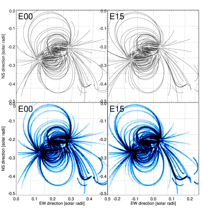
Figure 1.: Simulated pair of stereoscopic images E15 and E00, seen from an angle $15^{\circ}$ East from Earth (right bottom panel) and from Earth (left bottom panel). A heliographic coordinate grid is indicated with increments of $5^{\circ}$. The simulated EUV images are composed from 261 magnetic-field lines (top panels), generated from a potential-field extrapolation of a magnetogram of active region NOAA 11158 observed with HMI/SDO on 15 February 2011, 01:14 UT. Only field lines with magnetic field strengths of $|B_{z}|\geq 200$ G at the footpoints are displayed.

The barometric density is $n_{e}(h)\propto\exp(-h/\lambda)$, with the scale height $\lambda=50$ Mm $\times\ T_{e}$[MK], corresponding to a temperature of $T_{e}=2$ MK, which is typical for structures that are seen in the AIA 193 Å and 211 Å images. The intensity of the image scales with the emission measure, i.e. $F(x,y)\propto\int EM\ {\rm dz}\propto n_{e}^{2}\Delta z$, with $\Delta z$ the LOS-integrated column depth. For sake of simplicity, we do not intend to simulate AIA images at particular wavelengths, because the results of stereoscopic simulations depend primarily on the geometry and signal-to-noise ratio of the detected loops, which applies to any temperature or EUV wavelength.

In order to create an adequately realistic EUV image, we convolve each point of a field line with a Gaussian kernel that mimics typical loop aspect ratios (of the loop width to the length) and gravitational stratification. For the half width of a loop we choose the scaling of $w(s)=w_{0}\sqrt{n_{s}}$, where $n_{s}$ is the length of the loop in pixels, and $w_{0}=1$ Mm is the minimum loop width. In order to mimic the point spread function (PSF) of the instrument, we simulated loop widths [$w(s)$] with Gaussian kernels that are always larger than the PSF, i.e. $w(s)>w_{\rm psf}\approx$ two pixels.

Simulated EUV flux maps of the optically thin plasma are rendered in Figure 1 (bottom panels), similar to the method of Gary (1997). In the later sections of this article we also simulate similar EUV maps with different spacecraft-separation angles (section 6 and 7), with different spatial resolutions (section 8), or with different magnetic field models (section 10).

3 Automated Pattern Recognition

Stereoscopy of coronal structures has been pioneered only by visual tracing so far, for instance using Skylab images (Berton and Sakurai 1985) or STEREO/EUVI image pairs (Feng et al., 2007; Aschwanden et al. 2008). Manual tracing of coronal loops, however, is very time-consuming and depends on human judgement, and thus is very inefficient and subjective, preventing any frequent sampling or real-time operation. The availability of an automated pattern-recognition code is therefore a valuable element to accelerate progress in magnetic-field modeling of the solar corona. In our context here, we aim for a “blind stereoscopy method”, rather than “stereoscopy aided by visual guidance”.

Five experimental numerical codes for automated tracing of coronal loops were compared in an initial study (Aschwanden et al., 1998). One of them, the so-called oriented coronal curved loop tracing (OCCULT-1) code was further developed and approached visual perception (Aschwanden, 2010). A new advanced code (OCCULT-2) was further optimized for curvi-linear tracing applied to Transition Region and Coronal Explorer (TRACE) data (Handy et al., 1999), SDO/AIA data, Swedish Solar Telescope (SST) data, and microscopic biophysics images (Aschwanden, DePontieu, and Katrukha 2013). Here, we use this OCCULT-2 code. The automated pattern recognition algorithm detects iteratively curvi-linear patterns with large curvature radii, starting at a position with the highest flux, propagating along the local ridge guided by the local curvature radius, and it erases the signal of a traced loop segment from the image before it starts with the next loop segment. The automated loop tracings are carried out here independently in each image of a stereoscopic pair (such as E00, E15 shown in Figure 2).

Figure 2.: Automated loop tracing with the OCCULT-2 code (red curves), superimposed on the simulated 261 magnetic-field lines (black curves in top panels) and the simulated EUV images (bottom panels). A total of 80 (or 84) loop segments are detected at E00 (or E15) above a flux threshold of 1% and with a minimum length of $l_{\rm min}\geq 20$ pixels.

For an example, we show the automated tracing of a pair of simulated stereoscopic images in Figure 2, which was simulated using 261 magnetic field lines. The OCCULT-2 code detects from the EUV images a total of 80 loop segments with a length of $l_{min}\geq 20$ pixels in image E00, and 84 loop segments in image E15. The parameters can be adjusted depending on the type of data or desired pattern. What is particular about the simulated stereoscopic images here (Figure 1) is freedom from noise, in contrast to observed EUV images. Noise-free images allow for more sensitive detection of faint structures and are less prone to mis-guided detections in faint structures that are comparable with the ambient noise level. We simulate noise-free images here in order to study the performance of automated stereoscopy under ideal conditions, but will add data noise later to study the stereoscopic behavior under more realistic conditions.

For our application here we chose the following parameter settings for the code OCCULT-2: a pixel size of $1.5\hbox{${}^{\prime\prime}$}$ (or 1.0 Mm), a highpass filter of $nsm_{1}=1$ pixel, a minimum curvature radius of $r_{\rm min}=l_{\rm min}$ pixels, a minimum loop segment length of $l_{\rm min}=20$ pixels, an image base level of $thr_{1}=0$, a threshold level of $thr_{2}=0.01$ (in units of the highpass-filtered flux maximum), no gap ($n_{\rm gap}=0$) along a traced structure, and a maximum loop number of $n_{\rm max}=200$ loop structures per image. These settings yield a near complete detection of unconfused loop segments, down to the faintest structures seen visually (Figure 2). Since structures are generally seen down to the spatial resolution of the instrument, the same settings in units of pixels are recommended also for an instrument with a different spatial resolution (although it corresponds to a different absolute scale of the pixel size.) The most challenging part is the crowded central core of the active region, where multiple loops overlap and cross each other. A correct disentangling of loop structures in such nested areas can probably only be achieved by forward-fitting of multiple loop geometries, rather than by iterative loop tracing.

4 Automated Stereoscopic Pairing

The second major task of the autonomous stereoscopy procedure is the pairing of corresponding loops, namely the correct association of loop segment $i$ in image A with the stereoscopic counterpart of loop segment $j$ in the stereoscopic image B. This problem of “stereoscopic correspondence” or “stereoscopic pairing ambiguity” has never been systematically investigated, and thus we explore it here to some degree to enable automated stereoscopy.

Stereoscopy is generally accomplished by transforming a stereoscopic image pair into an epipolar coordinate system (Inhester 2006), which generally requires a rotation and rescaling of each image (if the images are taken with different image scales or at different distances from the Sun). The epipolar plane is defined by three points: the Sun center, and the positions of two stereoscopic vantage points, which are given by the spacecraft locations A and B for the solar STEREO mission. In such an epipolar coordinate system, an image A is taken in the $[x,y]$-plane, the epipolar rotation axis is in the $y$-direction, which warrants that the stereoscopic parallax causes a rotational shift in the $x$-direction only, while the $y$-coordinate remains unchanged. Consequently, any structure with coordinate $[x(s),y(s)]$ in image A, where $s$ is a loop-length coordinate, has the coordinates $[x(s)+\Delta x(\alpha_{s})+\Delta x(h),y(s)]$ in image B, where $\Delta x(\alpha_{s})$ is the rotational shift of the coordinate system due to the spacecraft-separation angle $\alpha_{s}$, and $\Delta x[h]$ is the parallax that depends on the altitude $h$ above the solar surface. The range of possible altitudes, $0\leq h\leq h_{\rm max}$, defines the solution space in image B, where a corresponding loop can be located. In the ideal case, a loop is detected over its entire length in both images, and appears isolated within the search area. The search area for such a loop with coordinates $[x_{1}(s),y_{1}(s)]$ in image A, is bound by $[x_{2}(s),y_{2}(s)]$ with $y_{1}(s)=y_{2}(s)$ in the $y$-direction and $x_{1}(s)\leq|x_{2}(s)-\Delta x(\alpha_{s})|\leq\Delta x(h_{\rm max})$ in the x-direction. If there is only one loop segment in this search area in image B, the correspondence is unique and a stereoscopic triangulation can directly be calculated. In reality, however, there are often multiple loops in the search area and we have to develop a strategy to find the most likely stereoscopically correct correspondence.

Figure 3.: The largest loop traced in image E00 (second panel from bottom) is #16 (black/white dashed linestyle), which corresponds to loop #9 in image W15 (bottom left panel), or to loop #35 in image E15 (bottom right panel). The projection of loops rotated at a photospheric level $h=0$ is indicated with blue curves, and rotated at a (maximum) coronal height of $h=0.15{\rm R}_{\odot}$ with red curves. The side views (top panels) indicate the stereoscopically triangulated altitudes of candidate loops in the solution space. The correct solution known from the simulated magnetic field is indicated with a field line drawn in orange color.

We illustrate the “stereoscopic correspondence problem” in Figure 3, where we show stereoscopy between a spacecraft W15 and Earth view (E00) (Figure 3 left panels), as well as stereoscopy between a spacecraft E15 and Earth view (E00) (Figure 3 right panels). A total of $n=80$ loops were detected in image (E00), while $84$ loop segments were detected in image (E15), whereof $n_{C}=51$ segments have an overlapping $y$-range in both images. The tracing of the largest loop in image E00, which has the number #16 when sorted by length, is outlined (black/white dashed linestyle) in Figure 3 in all panels. Rotating a loop structure from image E15 onto the view of E00, using two fixed distances from Sun center (i.e. with a minimum altitude $h=0$ and a maximum altitude of $h_{\rm max}=0.15{\rm R}_{\odot}$), we find a solution space in E00 for each structure detected in E15. In this case we find two loop segments that overlap with the traced loop #16 in image E00, so there is a two-fold ambiguity which loop should be stereoscopically triangulated. The boundaries of the solution space of loop #35 from image E15 is indicated in the image E00 with a red–blue zone, where blue corresponds to a minimum altitude of $h=0$ and red to a maximum altitude of $h=h_{\rm max}=0.15$ solar radii. Which is the correct correspondence? Since the probability of a true correspondence increases with the length of the coincident segment, we use the criterion of maximum length, which indeed corresponds to the correct solution (indicated with an orange line in the top panels), known from the simulated magnetic-field lines.

How large is the ambiguity of pairing stereoscopic loop segments? We count the number of loop segments in E15 to each loop segment of E00 that intersects with the stereoscopic solution space, bound by an overlapping y-range and altitude range $h=[0,h_{\rm max}]$. We find that most loops have an ambiguous stereoscopic correspondence, within a range of 1–10 possible correspondences, or a statistical mean of $n_{\rm amb}=3.2\pm 2.3$. In the example shown in Figure 3 (right panel), there are two ambiguous loop segments in image E15 that could potentially correspond to loop #16 in image E00 within the altitude range used. The degree of ambiguity generally depends on the specified altitude range, which is chosen to be $h_{\rm max}=0.15$ solar radii here, and is expected to linearly increase with larger altitude ranges. One strategy to reduce the number of ambiguities is to eliminate those that have already been used previously in the iterative stereoscopic pairing. A further strategy to avoid false stereoscopic pairings is to start with those that have the longest loop segments, where the least ambiguity occurs. Proceeding to smaller and smaller loop segments, the number of ambiguities then decreases systematically.

Based on these considerations, we implement the following steps in the (blind) stereoscopy code as a strategy to optimize the stereoscopic pairing procedure.

(i) All $n_{A}$ detected loops in A are sorted by their length.

(ii) All $n_{B}$ detected loops in B are sorted by their length.

(iii) For each sorted loop $i_{\rm A}=1,...,n_{\rm A}$ we determine which of the sorted loops $i_{\rm B}=1,...,n_{\rm B}$ overlap with the solution space of loop $i_{\rm A}$ within an altitude range of $h=[0,h_{\rm max}]$.

(iv) The longest segment in B that overlaps with the altitude range of loop $i_{\rm A}$ is selected as the stereoscopic counterpart $i_{\rm B,sel}$.

(v) A loop $i_{\rm B,sel}$ in B that has already previously been paired with a loop $i_{\rm A}$, is excluded for pairing in the next iterative pairing step.

An alternative approach to solve the loop correspondence problem is the so-called “magnetic stereoscopy method” (Wiegelmann et al., 2006; Feng et al., 2007), where an extrapolated linear force-free (LFFF) magnetic field is used to identify corresponding loops. A possible advantage of this method is that it reduces the solution space of corresponding loop locations more efficiently than our empirical stereoscopic pairing method described above, especially for large spacecraft-separation angles. However, a disadvantage of this method is that the initially chosen magnetic field (LFFF) model introduces a bias that favors solutions close to the initial (LFFF) model and may even prevent the convergence towards a nonlinear force-free field (NLFFF) solution. However, the best method may be an iterative approach, where stereoscopic loop pairing and magnetic field modeling is performed in alternating steps, starting from an initial potential field model, a and ideally ending at a best-fitting final non-potential field model.

5 3D-Triangulation of Loops

The third step in the blind-stereoscopy procedure consists of the triangulation of loop points. This is the easiest part of the stereoscopy procedure, because it is a uniquely defined mathematical geometry problem, after we have identified the correct corresponding loop counterparts in both images A and B in an epipolar coordinate system. Specific triangulation formula are given in a number of previous studies (e.g. Berton and Sakurai 1985; Inhester 2006; Aschwanden et al., 2008). Geometric parameters of the heliographic coordinate system of an image are generally specified in the FITS headers of the image data files (Thompson and Wei 2010).

Here, we derive the analytical relationships in their simplest form for a pair of two images A and B that have been already rotated and scaled into an epipolar coordinate system, which contains only four variables for every loop point $s$: $(x_{\rm A},y)$ are the coordinates of a loop point in image A with respect to the Sun center, $(x_{\rm B},y)$ are the coordinates of the corresponding loop point in image B, where the $y$-coordinate is identical in an epipolar coordinate system $(y=y_{\rm A}=y_{\rm B})$, and the stereoscopic spacecraft-separation angle [$\alpha_{s}$], measured from Sun center in the epipolar plane. Scaling the distances in units of solar radii, the distance from Sun center is $r=1+h$, where $h$ is the altitude above the solar surface. The distance of point $(x_{\rm A},y)$ from the solar (epipolar) axis is then

$$\rho=\cos{b}\ (1+h)\ ,$$ (1)

where $(l,b)$ are the heliographic longitude and latitude in a Stonyhurst grid (with $l=0$ and $b=0$ at solar disk center). The cartesian coordinates $x_{\rm A},y_{\rm A}$, $x_{\rm B}$ are then related to the heliographic coordinates $l_{\rm A},l_{\rm B},b$ by the following relationships,

$$x_{A}=\rho\ \sin{(l_{A})}\ ,$$ (2)

$$x_{B}=\rho\ \sin{(l_{B})}\ ,$$ (3)

$$l_{B}=l_{A}+\alpha_{s}\ ,$$ (4)

$$y=\sin{(b)}\ (1+h)\ .$$ (5)

Now we can substitute and eliminate the observables $(l_{\rm A},l_{\rm B},y)$ and obtain the relationships for the variables $(\rho,b,h$),

$$\rho=\left[x_{A}^{2}+\left({x_{B}-x_{A}\ \cos{\alpha_{s}}\over\sin{\alpha_{s}}}\right)\right]^{1/2}\ ,$$ (6)

$$b=\arctan{\left({y\over\rho}\right)}\ ,$$ (7)

$$h={\rho\over\cos{b}}-1\ .$$ (8)

Another simple method is to rotate the coordinate of a location $(x_{\rm B},y)$ from image B by the spacecraft angle $\alpha_{s}$ into the coordinate system of image A using two different altitudes [$h_{1}$ and $h_{2}$], so that the correct altitude $h$ can be interpolated at the matching position $x_{B}^{rot}=x_{\rm A}$. We used both methods in order to validate our triangulation code.

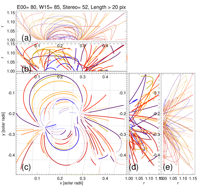
Figure 4.: Automatically traced loops in image E00 (thin colored curves) and loop segments with stereoscopic correspondences in E00 and E15 (thick colored curves) are shown in the $x-y$ plane (panel c). The stereoscopically triangulated solutions are shown in three projections, in the $x-r$ plane (panel b), and in the $r-y$ plane (panel d). The theoretical solutions known from the magnetic field simulations are shown in the panels a and e.

A result of stereoscopic triangulation of loops measured in the images E00 and E15 is shown in Figure 4, along with their projections into orthogonal planes. The 80 loop segments that were automatically traced in image E00 are displayed in Figure 4c (thin solid curves), while those segments for which a corresponding match in E15 was found are indicated with thick solid curves. The triangulated heights are shown as a function of the x-coordinate, $r(x)=1+h(x)$ (Figure 4b), and as a function of the y-coordinate, $r(y)=1+h(y)$ (Figure 4d). The closest matching 80 magnetic field lines that match the loops traced in image E00 are indicated also (Figure 4a and 4e). The display in Figure 4 demonstrates a good match between the theoretical magnetic field lines and the stereoscopically triangulated loops.

The numerical accuracy of stereoscopic triangulation depends somewhat on the spatial direction of the coronal loop or magnetic field line. In the epipolar coordinate system, the stereoscopic parallax occurs in the $x$-direction, which yields the most accurate measurement if a loop or field line is oriented in the y-direction, i.e. in the North-South direction. If the loop is oriented in the x-direction, there is a singularity in the altitude inversion, because the parallax direction coincides with the loop direction, and the correspondence of a loop segment in a pair of two stereoscopic images is mathematically ill-defined, which prohibits stereoscopic triangulation at this location. This singularity, which we may call the “epipolar degeneracy”, can affect the accuracy of stereoscopic triangulation for a range of angles where the tilt-angle $\tan(|\vartheta(s)|)=|y(s_{i+1})-y(s_{i})|/|x(s_{i+1})-x(s_{i})|$ along a loop coordinate $s$ has a small value, due to the finite spatial resolution and directional tracing errors (Aschwanden et al., 2008, 2012b). In order to overcome this epipolar degeneracy problem, we apply stereoscopic triangulation only at loop locations [$s$] where the loop direction is larger than a critical value, i.e., $|\tan{\vartheta(s)}|\geq 0.1$, and apply a low-order polynomial interpolation for the coordinate $z(s)$ in those gaps.

6 Dual Versus Triple Spacecraft Stereoscopy

The minimum option for solar stereoscopy is two perspectives, but one may opt for a third for a number of reasons. First of all, should one instrument fail, one has still a fall-back option with two spacecraft that can essentially accomplish the stereoscopy task. Secondly, stereoscopy with two perspectives often confronts us with the problem of ambiguous correspondence. Which loop structure from perspective A has to be triangulated with what loop structure from perspective B? The combination of three perspectives virtually eliminates the stereoscopic-ambiguity problem.

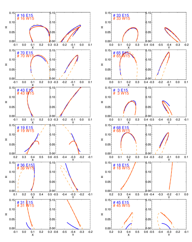
Figure 5.: Comparison of solutions for altitudes as a function of the $x$-coordinate, $h(x)$, and the $y$-coordinate, $y(h)$, from the stereoscopic triangulation between the images E00 and E15 (blue curves), and the images E00 and W15 (red curves). The theoretical solutions based on the closest simulated magnetic-field lines are indicated in orange. Inconsistent solutions occur for four loops (#18, 19, 31, 45) out of the 12 cases, but are correct for the spacecraft image W15 (red curves) in all cases but #19.

We demonstrate the bootstrapping effect of stereoscopic triangulation as it could be achieved with three spacecraft in the example shown in Figure 5. The view of the active region from the three spacecraft E00, E15, and W15 is depicted in Figure 3, and stereoscopy of loop #16 from the image pair E00 and E15 (Figure 3 right panels), and the pair E00 and W15 (Figure 3 left panels) yields a self-consistent solution that is close to the theoretical values (orange curves in Figure 3). In Figure 5 (top left panels) we show the orthogonal projections $h(x)$ and $h(y)$ for the same loop #16, found from the spacecraft pair E15+E00 (Figure 5, blue curves), and from the spacecraft pair W15+E00 (Figure 5, red curves), along with the theoretical solution (Figure 5, orange curves in dashed linestyle), which all agree within $\Delta h\lower 1.72218pt\hbox{$\;\buildrel<\over{\scriptstyle\sim}\;$}0.01$ solar radii. In the same representation we show the same information for the 12 longest detected loops in Figure 5. From these 12 stereoscopic triangulations we see a consistent solution of both spacecraft pairs with the theoretical model field lines in eight cases, while the results from E15+E00 (Figure 5, blue curves) fail for the four loops #18, 19, 31, and 45. Nevertheless, the results from W15+E00 are correct in 11 out of 12 cases. For this particular example, which may be typical for many other observations, we can say that stereoscopic triangulation with three spacecraft is successful in $\approx 90\%$ (11 out of 12 cases), while triangulation with two spacecraft can have a reduced success rate in the range of 75%–90%, depending on the position of the spacecraft. A generalization of our two-spacecraft stereoscopy code to a triple-spacecraft configuration could easily be implemented, based on the relative overlap range of the $y(s)$-values of the automatically traced loop segments in each of the three spacecraft images, and the highest probability or correct stereoscopic correspondence based on the maximum lengths of the paired loop segments among the three images from different vantage points.

7 Spacecraft Separation Angle

What is the optimum spacecraft-separation angle for stereoscopy? In a previous study with STEREO/EUVI data, it was demonstrated that stereoscopic triangulation is in principle possible from small ($6^{\circ}$) to large ($170^{\circ}$) angles, based on a small sample of visually traced loops (Aschwanden et al., 2012b). Combining the accuracy of altitude triangulation with the stereoscopic correspondence ambiguity, it was estimated that a spacecraft-separation angle of $\alpha_{s}=22^{\circ}-125^{\circ}$ is most favorable for stereoscopy, using an instrument with the spatial resolution $2.6\hbox{${}^{\prime\prime}$}$ (with pixel size of $1.6\hbox{${}^{\prime\prime}$}$) such as STEREO/EUVI.

Here, we simulate data for a spacecraft-separation angle of $\alpha_{s}=1^{\circ}$ to $90^{\circ}$ in both the eastern and western direction, and perform stereoscopic triangulation between a spacecraft at angle $\alpha_{s}$ (W90,…,W01, E01, …E90) and the spacecraft at Earth view (E00). For simplicity we label the positions at angles (W90,…,W01, E01, …E90) with “spacecraft A”, and the position at Earth view with “spacecraft E”.

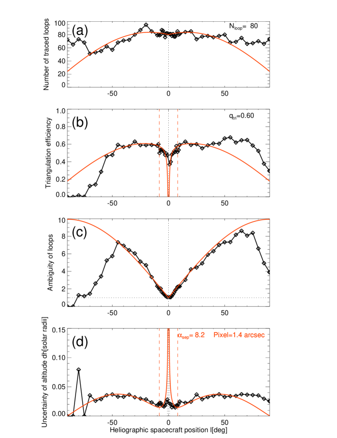
Figure 6.: (a) Statistics of the number of automatically traced loops (top panel), (b) the number of triangulation points (second panel), (c) the mean number of ambiguous loops per triangulated loop, given by the mean and standard deviation (third panel), and (d) the median accuracy of altitude measurements $dh$ in units of solar radii, as a function of the spacecraft heliographic position (or spacecraft-separation angle from Earth). The colored curves correspond to the theoretical model described in the text. The spatial resolution corresponds to a pixel size of $\Delta x=1.4\hbox{${}^{\prime\prime}$}$.

For each of the spacecraft positions we measure the number of automatically traced loops (Figure 6a), which has a maximum value of $N_{0}=80$ (in image E) and tends to decrease as the region is seen closer to the solar limb (in the images A). If the distribution of loops were homogeneous and isotropic in an active region, the view would be rotation-invariant and the number of detected loops should be constant as a function of the aspect angle. Therefore, the observed slight decrease of detected loops towards the limb indicates a larger horizontal than vertical extent of the active region. If we assume a homogeneous density of loops in a box with a horizontal length [$\Delta x$] and height [$h_{\rm max}$], the projected length of the box as a function of the rotation angle (or longitude) $\alpha_{s}$, we expect that the number of detected loops is roughly proportional to the projected length of the box, for which we then expect a center-to-limb variation of

$$N_{loop}(\alpha_{s})\approx N_{0}{\Delta x\cos{(\alpha_{s})}+h_{max}\sin{(\alpha_{s})}\over{\Delta x}}\ ,$$ (9)

where $N_{0}$ is the maximum number of detected loops, $\Delta x$ is the East–West extension of the active region, and $h_{max}$ is the maximum altitude. We overplot such a function in Figure 6a, using $\Delta x=0.5{\rm R}_{\odot}$ based on the chosen field-of-view, and $h_{max}\approx 0.15{\rm R}_{\odot}$, which approximately reproduces the decrease of detected loops towards the limb. The AR is located at $12^{\circ}$ West, causing an obscuration by the limb at $-78^{\circ}$ and the number of detected loops to go to zero beyond the limb.

Then we measure the triangulation efficiency $q_{\rm tri}$ in suitable loop segments (Figure 6b). This number is defined by the ratio $q_{\rm tri}=N_{\rm tri}/N_{\rm all}$ of the number of loop positions $N_{\rm tri}$ where a valid stereoscopic triangulation could be executed, normalized to the total number $N_{\rm all}$ of all possible loop positions. The requirement for a stereoscopic triangulation of a loop position is a valid stereoscopic correspondence between two spacecraft A and E, which is an identical $y$-position in both spacecraft A and E, and a valid altitude range of $0\leq h\leq h_{\rm max}$ in the stereoscopic triangulation. For this number we find a typical value of $q_{tri}\approx 0.5$, mostly caused by incomplete loop tracing or erroneous stereoscopic correspondence identifications. As we can see in Figure 6b, the number of triangulated loop positions $q_{\rm tri}(\alpha_{s})$ follows a similar function as the number of detected loops (Equation 9), with a drop-off at both the eastern and western limb. Thus the efficiency of stereoscopy is warranted in a broad range of $|\alpha_{s}-l_{0}|\lower 1.72218pt\hbox{$\;\buildrel<\over{\scriptstyle\sim}\;$}60^{\circ}$ between a spacecraft position A and E, where $l_{0}\approx 12^{\circ}$ is the longitude of the active region.

Figure 7.: The number of ambiguous loops in stereoscopic correlation as a function of the spacecraft-separation angle [$\alpha_{s}$] is shown. If spacecraft A located at $\alpha=0^{\circ}$ detects one single loop within a spatial width of $\Delta x=1$, a spacecraft B at position $\alpha=90^{\circ}$ detects a number of $N_{\rm amb}(\alpha)=\sqrt{N}$ loops that all have the same projection after they have been rotated by an angle of $-\alpha$ to the viewpoint of spacecraft A in the $z$-direction. For an intermediate position B at $\alpha$, the number of ambiguous loops scales as $N_{\rm amb}(\alpha)=\sqrt{N}\sin(\alpha)$.

The number of ambiguous loops may also play a significant role in the evaluation of the optimum spacecraft angle for stereoscopy. We performed automated stereoscopy between a near-Earth spacecraft E and a spacecraft A at any position from the most western viewpoint at $\alpha_{s}=-90^{\circ}$ to the most eastern viewpoint $\alpha_{s}=+90^{\circ}$, in increments of $5^{\circ}$ for the whole range, and in increments of $1^{\circ}$ in the small-angle range of $-10^{\circ}\leq\alpha_{s}\leq+10^{\circ}$. While the automated code detected $N_{\rm loop}=80$ loop structures in image E, an average number of $1\leq n_{\rm loop,A}\lower 1.72218pt\hbox{$\;\buildrel<\over{\scriptstyle\sim}\;$}10$ ambiguous loops were detected in image A, where “ambiguous” means the number of candidate loops in image A that have a valid altitude range $0\leq h\leq h_{\rm max}=0.15$ in the stereoscopic triangulation. The variation of the number of ambiguous loops is shown in Figure 6c, which reveals a minimum of one single loop at $\alpha_{s}\approx 0^{\circ}$, while the ambiguity seems to increase up to angles of $\alpha_{s}\approx 50^{\circ}-70^{\circ}$. We can model the number of ambiguities by assuming a uniform distribution of North-South oriented loops in a cube, which is most favorable for stereoscopy (Figure 7). If we have $n_{x}$ loops in $x$-direction and $n_{h}$ loops in $h$-direction, the total number of loops is $N_{\rm loop}=n_{x}\times n_{h}$. For a quadratic box with a maximum number $N_{\rm loop}$ of detected loops we have $n_{x}=n_{h}=\sqrt{N_{\rm loop}}$. The number of ambiguous loops scales then with the projected length ($\Delta x$ in Figure 7) as a function of the rotation angle (or spacecraft-separation angle $\alpha_{s}$). If a loop were detected within a width of $\Delta x=1$ (Figure 7) for a small stereoscopic viewing angle, the projected width of all stereoscopically corresponding loops is $\Delta x\approx\sqrt{N}$ at the limb (Figure 7), and scales according to the sine-function inbetween,

$$n_{amb}(\alpha_{s})=1+\sqrt{N_{loop}}\ \sin{|\alpha_{s}|}\ ,$$ (10)

which is overplotted on the measurements in Figure 6c. The predicted number of ambiguous loops matches the numerically determined number fairly accurate over the range of $-50^{\circ}\lower 1.72218pt\hbox{$\;\buildrel<\over{\scriptstyle\sim}\;$}\alpha_{s}\lower 1.72218pt\hbox{$\;\buildrel<\over{\scriptstyle\sim}\;$}80^{\circ}$. The ambiguity factor is almost symmetrical for a western and eastern separation angle, but exact symmetry is not expected for an active region that has no symmetry in its magnetic field and EUV brightness.

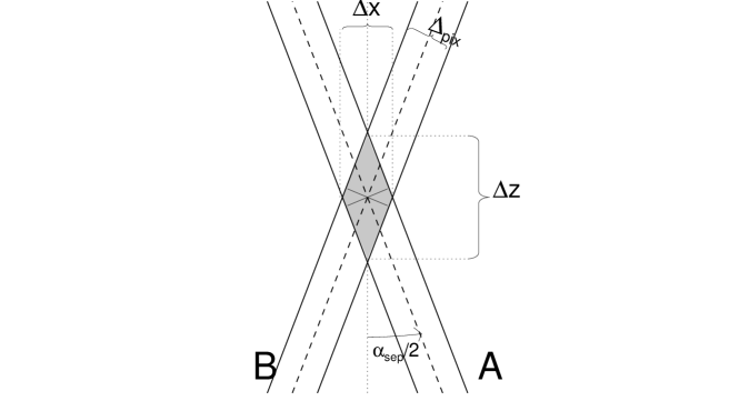
Figure 8.: The error trapezoid of stereoscopic triangulation is shown (grey area), given by the two lines of sight of the two observer directions A and B, separated by an angle $\alpha_{s}$. The uncertainties [$\Delta x$] in the $x$-direction and in the $z$-direction depend on the pixel width [$\Delta_{\rm pix}$] and half aspect angle $\alpha_{s}/2$ (Aschwanden et al., 2012b).

The ultimate parameter that determines the optimum spacecraft-separation angle for for dual-spacecraft stereoscopy is the accuracy of altitude measurements, which depends not only on the ambiguity factor (for stereoscopic correspondence) but also on the spatial resolution of the images. If we make the spacecraft-separation angle smaller and smaller, the horizontal parallax as a function of the altitude becomes also smaller and will reach sub-pixel scale, where the stereoscopic information becomes unmeasurable, because there is a singularity when the spacecraft-separation angles approach zero. Theoretically, the error in the line-of-sight extent [$\Delta z$] of a point source observed with a spatial resolution [$\Delta x$] can be understood from the “trapezoid relationship” (Aschwanden et al., 2012b) shown in Figure 8,

$$\Delta h_{res}={\Delta x/2\over\sin{(|\alpha_{s}|/2)}}\ ,$$ (11)

which exhibits a singularity at spacecraft-separation angle $\alpha_{s}=0$ in the number of stereoscopic triangulation points (Figure 6b) and in the accuracy [$\Delta h$] (Figure 6d) of stereoscopically triangulated altitudes. For larger spacecraft-separation angles, this finite spatial resolution effect becomes negligible, while uncertainties due to the ambiguity factor in stereoscopic correspondence dominate. Thus, the center-to-limb variation of the accuracy of altitude measurements is expected to vary as a sine-function as the ambiguity function does (Equation 10), where the maximum (positive or negative) error corresponds to the half height range ($h_{\rm max}/2)$,

$$\Delta z_{amb}={h_{max}\over 2}\sin{(|\alpha_{s}|)}\ .$$ (12)

In order to obtain an error in altitude [$\Delta h$], we have to correct for the cosine-angle of the projection between the line-of-sight $z$ and the altitude $h$,

$$\Delta h_{amb}=\Delta z_{amb}\ \cos{|\alpha_{s}|}\ ,$$ (13)

which yields the combined error (added in quadrature),

$$\Delta h=\sqrt{\Delta h_{res}^{2}+\Delta h_{amb}^{2}}=\left[\left({\Delta x/2)\over\sin{(|\alpha_{s}|/2)}}\right)^{2}+\left({h_{max}\over 2}{\sin{\alpha_{s}}\cos{\alpha_{s})}}\right)^{2}\right]^{1/2}\ .$$ (14)

This theoretical prediction is overplotted on the numerical datapoints of the uncertainties for the stereoscopic altitude measurements (Figure 6d, red smooth curve), which matches the data closely in the range of $-60^{\circ}\leq\alpha_{s}\leq+60^{\circ}$. An interesting consequence of this model is that it predicts a highest accuracy at a spacecraft separation angle of $\alpha_{s}\approx 8.2^{\circ}$. According to the simulations, the highest accuracy is $\Delta h\approx 0.02{\rm R}_{\odot}$ (or 14 Mm), does not deteriorate more than about a factor of two to $\Delta h\lower 1.72218pt\hbox{$\;\buildrel<\over{\scriptstyle\sim}\;$}0.04{\rm R}_{\odot}$ (or 28 Mm) at larger separation angles.

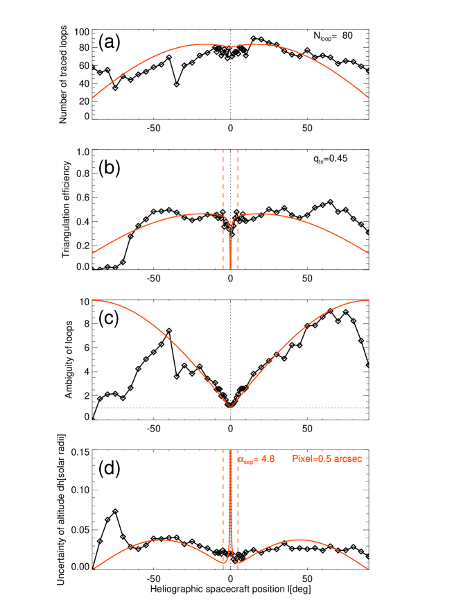
Figure 9.: Same representation as Figure 6, but for a spatial resolution corresponding to a pixel size of $\Delta x=0.6\hbox{${}^{\prime\prime}$}$): (a) Statistics of the number of automatically traced loops (top panel), (b) the number of triangulation points (second panel), (c) the mean number of ambiguous loops per triangulated loop, given by the mean and standard deviation (third panel), and (d) the median accuracy of altitude measurements $dh$ in units of solar radii, as a function of the spacecraft heliographic position (or spacecraft-separation angle from Earth).

This is also the reason why a relatively wide range of stereoscopic angles of $\alpha_{s}\approx 22^{\circ}-125^{\circ}$ was found to be usable for stereoscopy according to an earlier study (Aschwanden et al., 2012b), a range that has been adopted for another proposed future stereoscopic mission (Strugarek et al., 2015). Note that the uncertainty of the ambiguity was estimated differently in the previous study, assuming a dependence of $\Delta h_{\rm amb}\propto 1/|\cos{(\alpha_{s})}|$ based on a theoretical argument (Equation 7 in Aschwanden et al., 2012b), while we obtain a probably more realistic dependence of $\Delta h_{\rm amb}\propto\sin{(\alpha_{s})}\cos{(\alpha_{s})}$ (Equations 12 and 13) here, based on numerical simulations of stereoscopic triangulations. The large range of $\alpha_{s}=22^{\circ}-125^{\circ}$ still specifies an angular range where stereoscopy is feasible, if we tolerate a factor of two in the uncertainty of altitude measurements (Figure 6d and 9d), but the optimum angle of $4.6^{\circ}-10.7^{\circ}$ found here (Table 1) yields the most precise measurements according to our simulations.

Table 1.: Dependence of optimum spacecraft-separation angle [$\alpha_{\rm best}$] and the uncertainty of stereoscopic altitudes [$\Delta h$] on the spatial resolution [$\Delta x$] and altitude range [$h_{\rm max}$] of the solution space.

Instrument	Pixel	Spatial	Pixel	Altitude	Spacecraft	Altitude
	size	resolution	size	range	separation	uncertainty
					angle
	$\Delta x$	PSF	PSF	$h_{max}$	$\alpha_{best}$	$\Delta h$
	[arcsec]	[arcsec]	[Mm]	[Mm]	[deg]	[Mm]
AIA	0.6	1.4	0.44	70	6.3∘	5.5
EUVI	1.6	2.6	1.16	70	10.7∘	8.9
AIA	0.6	1.4	0.44	140	4.6∘	7.8
EUVI	1.6	2.6	1.16	140	7.4∘	12.6

8 Spatial Resolution

The accuracy of stereoscopic altitude measurements apparently depends on the spatial resolution $\Delta x$ of the instrument, the spacecraft-separation angle $\alpha_{s}$, and the altitude range $h_{\rm max}$ of the solution space, according to the relationship of Equation (14), and thus the best spacecraft-separation angle depends on the same parameters [$\Delta x$] and [$h_{\rm max}$]. We determined the minimum of the function $\alpha_{s}(\Delta x,h_{\rm max})$ numerically and tabulate the values for $\Delta x=0.6\hbox{${}^{\prime\prime}$},1.6\hbox{${}^{\prime\prime}$}$ and $h_{\rm max}=[0.1,0.2]{\rm R}_{\odot}$ in Table 1. The coarsest spatial resolution of $2.6\hbox{${}^{\prime\prime}$}$ (with pixel size of $1.6\hbox{${}^{\prime\prime}$}$) corresponds to the EUVI/STEREO instruments, and $1.4\hbox{${}^{\prime\prime}$}$ (with pixel size of $0.6\hbox{${}^{\prime\prime}$}$) to the SDO/AIA instrument with $4k\times 4k$ CCD cameras.

The values in Table 1 show that the spacecraft-separation angle increases from $\alpha_{\rm best}=6.3^{\circ}$ to $\alpha_{\rm best}=10.7^{\circ}$ for the altitude range of $h_{\rm max}=0.1{\rm R}_{\odot}$, while the accuracy of the stereoscopically triangulated altitudes worsens steadily from $\Delta h=5.5$ Mm to 8.9 Mm. Thus, the highest accuracy is clearly achieved for the instrument with the highest spatial resolution, as expected. We can derive an approximate relationship for the optimum spacecraft-separation angle $\alpha_{\rm best}$ by setting the uncertainty due to the spatial resolution ($\Delta h_{\rm res}$; Equation 11) equal to the uncertainty due to loop pairing ambiguities ($\Delta h_{\rm amb}$; Equation 12 and 13). For small spacecraft-separation angles we can then use the approximations $\sin(\alpha_{s})\approx\alpha_{s}$, and $\cos(\alpha_{s})\approx 1$, which yields the relationship

$$\alpha_{best}\approx\sqrt{2\Delta x\over h_{\rm max}}\ ,\qquad[{\rm rad}],$$ (15)

which tells us that the spacecraft-separation angle [$\alpha_{s}$] scales with the square root of the spatial resolution [$\Delta x$]. Varying the altitude range $h_{\rm max}$ by a factor of two, the stereoscopic accuracy worsens a factor of $\sqrt{2}$. Thus, for a typical range of $h_{\rm max}\approx(0.1-0.2){\rm R}_{\odot}$, and for a pixel size $0.6\hbox{${}^{\prime\prime}$}$ (i.e. $\Delta x=0.000625$) as used for the AIA instrument, the optimum spacecraft-separation angle is $\alpha_{\rm best}\approx 4.6^{\circ}-6.3^{\circ}$. We repeat the calculations, shown for a spatial resolution of $1.6\hbox{${}^{\prime\prime}$}$ shown in Figure 6, for the AIA spatial resolution of $0.6\hbox{${}^{\prime\prime}$}$ in Figure 9. If we use the existing STEREO/EUVI instruments with a spatial resolution of $2.6\hbox{${}^{\prime\prime}$}$ (with pixel size of 1.6^′′, or $\Delta x=0.0017$), the optimum spacecraft-separation angle would be in the range of $\alpha_{s}\approx 7.4^{\circ}-10.7^{\circ}$ (Table 1).

9 Spacecraft Position

Considering the functional behavior of $\Delta h(\alpha_{s})$ as shown in Figures 6 and 9, we also expect a minimum of the stereoscopic error at large angles of $\alpha_{s}=\pm 90^{\circ}$. This solution corresponds to an orthogonal view of an active region, where the $x$ and $z$ position of a loop can be measured with maximum accuracy. This large-angle configuration, however, has at least three major disadvantages compared with the optimum small-angle configuration: (i) Obscuration by the solar limb has a much higher probability that an active region is not seen simultaneously by two spacecraft; (ii) The stereoscopic correspondence ambiguity is much more severe at large spacecraft angles than at small ones; and (iii) A large spacecraft distance from Earth demands a much higher telemetry power. For instance, a spacecraft-separation angle of $\alpha_{s}=6^{\circ}$ implies a ten times smaller proximity to Earth than a spacecraft position of $\alpha_{s}\approx 60^{\circ}$ at Lagrangian points L4 or L5, and thus enables a 100 times higher telemetry rate, or a 100 times smaller telemetry power for the same data rate.

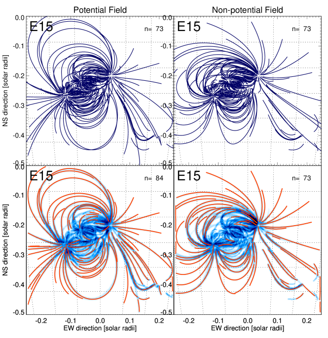
Figure 10.: Automated loop tracing with the OCCULT-2 code (red curves), superimposed on the simulated magnetic field lines (blue curves in top panels) and the simulated EUV images (bottom panels). The left panels show a potential field, while the right panels show a non-potential field. Note that the tracings of loops in the EUV images (bottom) are significantly different for the potential and non-potential fields, which proves that our automated method is very sensitive to the degree of the magnetic non-potentiality.

10 Non-Potentiality of Magnetic Field

The ultimate goal of a new stereoscopy mission is a reliable and accurate method to measure the magnetic field of solar active regions in order to monitor the evolution of non-potential fields and to determine their free energy that can be released in large solar flares and coronal mass ejections. The question arises then, whether the proposed automated tools are sufficiently accurate for this task. We may ask whether a stereoscopy method is sufficiently sensitive to distinguish between a potential and non-potential magnetic field, and how accurately can it measure the degree of non-potentiality. For a qualitative demonstration we simulate the magnetic field for a potential field, using 100 unipolar magnetic charges to represent the field (Figure 10; top left), and simulate a corresponding EUV image in the same way as described above (Figure 10; bottom left), to which then our OCCULT-2 code is applied to trace the loops in an automated way (red curves in Figure 10, bottom left).

Then we use the same model with 100 unipolar magnetic charges, but add a vertical electric current to the strongest magnetic charge, which has a magnetic-field strength of -2070 G and is located at $(x,y,z)=(-0.13,-0.26,0.95)$ (see left-most sunspot in Figure 10) by assigning a force-free parameter $\alpha$-parameter of $\alpha_{1}=2\pi N_{\rm twist}/L=10^{-9}$ cm^-1. The method of parameterizing the nonlinear force-free field is identical to that of the parameterization used in the simulation of the magnetic-field data described in section 3 (Aschwanden et al., 2012a). Comparing this non-potential field (Figure 10; top right) with the potential field (Figure 10; top left) one can see that the non-zero $\alpha$-parameter induces a helical twist in the eastern-most sunspot, which causes the field lines emanating from the sunspot to be rotated by some amount in the anti-clockwise direction. The bottom panels in Figure 10 clearly demonstrate that the automated loop tracing code picks out significantly different geometries for the two cases, so that we expect a significantly different magnetic field solution, once 3D nonlinear force-free modeling is attempted.

Using the vertical-current model for non-potential magnetic fields (i.e., Priest 1982; 2014; Aschwanden 2013a), the azimuthal angle [$\mu$] of a helically twisted magnetic field line scales proportionally to the number $N_{\rm twist}$ of twists and reciprocally to the length $L$ of the magnetic-field line,

$$\tan{(\mu)}={2\pi RN_{twist}\over L}=\alpha R\ ,$$ (16)

where $R$ is the flux-tube radius, and $\alpha$ is the nonlinear force-free parameter. From the examples of loop tracing using our OCCULT-2 code, as shown in Figure 2, we can estimate that the deviation of tracing from a true magnetic-field line is less than about one pixel for a loop length of more than 100 pixels. Thus, from $\tan{(\mu)}\lower 1.72218pt\hbox{$\;\buildrel<\over{\scriptstyle\sim}\;$}0.01$ and $R\approx$ one pixel, we find a lower limit of the force-free parameter $\alpha=\tan({\mu})/R\approx 1\times 10^{-10}$ cm^-1. This is an estimate of the sensitivity of our automated loop-tracing code to the non-potentiality of the magnetic field. This is commensurable with a range of $\alpha$-values found in flare-prone regions, e.g. $|\alpha|\lower 1.72218pt\hbox{$\;\buildrel<\over{\scriptstyle\sim}\;$}0.02$ arcsec${}^{-1}\approx 3\times 10^{-10}$ cm^-1; see Figure 3 in Malanushenko et al., 2014).

11 Discussion and Conclusions

We developed an automated stereoscopy code that reconstructs the 3D geometry of coronal loops in a solar active region based on EUV images, observed with two or three spacecraft located in feasible orbits, i.e. at about 1 AU from the Sun, either ahead or trailing behind Earth. In principle, such a “blind stereoscopy” algorithm can be applied to already existing spacecraft data, such as from SDO/AIA and STEREO/EUVI-A(head) and B(ehind), but these existing spacecraft missions have neither an optimum geometric configuration nor optimum spatial resolution of the instruments. We therefore explored the optimum conditions for a future mission that may place dual spacecraft anywhere between a near-Earth position and the Lagrangian L4 and L5 points. From our study we arrive at the following conclusions:

i) Spatial Resolution: The accuracy of stereoscopic triangulation scales directly proportional to the spatial resolution of the EUV imager for a given spacecraft-separation angle, i.e. the uncertainty or error $\Delta h_{\rm res}\propto\Delta x$ (Equation 11). It is therefore desirable to have the highest possible spatial resolution. A combination of requirements of full-Sun coverage, high S/N, telemetry, and available space-qualified CCD detectors, plus an existing EUV Earth-perspective imager already on orbit suggests that a pixel size of $0.6\hbox{${}^{\prime\prime}$}$ for a $4k\times 4k$ imager as implemented in the current SDO/AIA instrument is suitable for the purpose of stereoscopic loop tracing.

ii) Number of Spacecraft: Minimum stereoscopy can be performed with a pair of two spacecraft, for instance a spacecraft with one AIA-like telescope at a stereoscopic vantage point, in combination with the existing AIA spacecraft in a near-Earth orbit. However, a three-spacecraft configuration, such as the existing AIA and two twin spacecraft located ahead of and behind the Earth would substantially reduce ambiguities in the stereoscopic correspondence problem, as well as provide redundancy in case of any one instrument failing.

iii) Stereoscopic Correspondence or Ambiguity Problem: From the simulations of synthetic images of active regions we found that the number of stereoscopically corresponding loops (detected in an image pair from a spacecraft A and B) increases linearly with the spacecraft-separation angle $\alpha_{s}$. This means that larger separation angles lead to increased mapping ambiguity. Thus we should aim for the smallest possible angle where stereoscopy is feasible. In contrast, large-angle stereoscopy, although feasible, is not at optimum conditions. The minimization of the spacecraft-separation angle implies also an optimum telemetry rate, since the signal weakens with the squared distance to Earth.

iv) Optimum Spacecraft Separation Angle: The number of ambiguous loops and thus the uncertainty of stereoscopic triangulated altitudes increases roughly linearly with the separation angle, i.e. $\Delta h_{\rm amb}\propto\sin(|\alpha_{s}|)$ (Equation 12) for small angles. On the other hand, the uncertainty of stereoscopic triangulated altitudes decreases reciprocally with the spacecraft-separation angle due to the limited spatial resolution of the instrument, i.e. $\Delta h_{\rm res}\propto 1/sin{|\alpha_{s}|}$ (Equation 11). The best compromise between these two competing effects is at a spacecraft separation angle $\alpha_{\rm best}$ where the two uncertainties are comparable, i.e. $\alpha_{best}\approx\sqrt{2\Delta x/h_{\rm max}}$ (Equation 15), which yields $\alpha_{\rm best}=4.6^{\circ}-6.3^{\circ}$, for an altitude limit of $h_{\rm max}=0.1-0.2$ $R_{\odot}$. The altitude limit defines the vertical extent of the 3D solution space in stereoscopic triangulations.

v) Magnetic Non-Potentiality: We performed a qualitative test of how sensitive our automated stereoscopy is to the magnetic topology of potential and non-potential fields and found that the uncertainties of automated loop tracing (in the $xy$-plane) has sub-pixel accuracy, while the displacements of loops between a magnetic potential and non-potential field is much larger (of order $\lower 1.72218pt\hbox{$\;\buildrel<\over{\scriptstyle\sim}\;$}0.1R_{\odot}$), and thus our automated stereoscopy code is sufficiently sensitive to changes in the nonlinear force-free field geometry, down to a nonlinear force-free parameter of $\alpha\lower 1.72218pt\hbox{$\;\buildrel>\over{\scriptstyle\sim}\;$}10^{-10}$ cm^-1.

Our study complements and augments other recent mission concepts that are proposed as platforms to support space weather research and operations. One such mission is an L5 Lagrangian Point capability (Vourlidas, 2015) which focuses on the propagation of CMEs through the high corona and into the solar wind out to Earth, focusing primarily on the observation and eventual modeling of the time and velocity of arrivals of CMEs at Earth. The goals of such an L5 mission would clearly benefit from a better specification of the Sun–heliosphere field interface, for instance by adding magnetograph capabilities to increase the coverage of the solar surface. At this point, the proposed concept recognizes that ”the entrained magnetic field of an Earth-directed CME is beyond the reach of current remote-sensing capabilities.”

The goal of the present article is to open up a pathway that addresses that problem by developing, at least in principle, the methodology to obtain the information needed for active-region field modeling based on stereoscopic measurements. Another proposed mission concept, OSCAR (Strugarek et al., 2015), for example, also explores that through a perspective from somewhere around L5. OSCAR’s premise is that a suitable stereoscopy angle lies in the range of $\approx 22^{\circ}-125^{\circ}$, based on an earlier work by Aschwanden et al., (2012b).

The earlier study by Aschwanden et al., (2012b) developed a “quality” metric for stereoscopy, which included a plausibility argument for the ambiguity of loop tracing. Here, we quantify a metric for ambiguity directly from the loop-correspondence algorithm tested here, based on simulated coronal images of an active region from different perspectives. A result of the blind-stereoscopy algorithm developed here is that the best performance in resolving the stereoscopic correspondence ambiguity is found for considerably smaller spacecraft-separation angles of $\approx 5^{\circ}$. At such small angles, the highest accuracy is found for coronal stereoscopy to constrain nonlinear force-free modeling of coronal magnetic fields. This low separation angle, additionally offers the advantage of a higher telemetry rate for a given spacecraft and ground-antenna combination.

With these findings we realize that any space-weather mission concept has to deal with the trade-offs between small-angle stereoscopy, large-angle CME coverage, and spacecraft telemetry. An optimum configuration that meets the scientific and operational needs to study CMEs both in terms of magnetic content and in terms of their propagation through the heliosphere (cf., Schrijver et al., 2015) would appear to substantially benefit from having a triplet spacecraft configuration that includes both the L1 and L5 point, and a third spacecraft about $5^{\circ}$ away from Earth, equipped with complementary capabilities to measure the magnetic field, the plasma parameters, the arrival velocity, and the arrival time of Earth-bound (geoeffective) CMEs.

Part of the work for automated loop tracing was supported by the NASA contracts NNG04EA00C of the SDO/AIA instrument. We also acknowledge Lockheed Martin (LM) independent research funding supporting the stereoscopic aspects.

Disclosure of Potential Conflicts of Interest

The authors declare that they have no conflicts of interest.

References

Aschwanden, M.J., Lee, J.K., Gary, G.A., Smith, M., Inhester, B. 1998, Solar Phys. 248, 359.

Aschwanden, M.J., Newmark, J.S., Delaboudinière, J.P., Neupert, W.M., Klimchuk, J.A., Gary, G.A., Portier-Fornazzi, F., Zucker,A. 1999, Astrophys. J. 515, 842.

Aschwanden, M.J., Alexander, D., Hurlburt, N., Newmark, J.S., Neupert, W.M., Klimchuk, J.A., G.A. Gary 2000, Astrophys. J. 531, 1129.

Aschwanden, M.J., Wülser, J.P., Nitta, N., Lemen,J. 2008, Astrophys. J. 679, 827.

Aschwanden, M.J. 2010, Solar Phys. 262, 399.

Aschwanden, M.J., Sandman, A.W. 2010, Astron. J.  140, 723.

Aschwanden, M.J. 2011, Living Rev. Solar Phys. 8, 5, DOI: 10.12942/lrsp-2011-5.

Aschwanden, M.J., Wuelser, J.P., Nitta, N.V., Lemen, J.R., Schrijver, C.J., DeRosa, M., Malanushenko, A. 2012a, Astrophys. J. 756, 124.

Aschwanden, M.J., Wuelser, J.P., Nitta, N.V., Lemen, J.R., 2012b, Solar Phys. 281, 101.

Aschwanden, M.J. 2013a, Solar Phys. 287, 323.

Aschwanden, M.J. 2013b, Astrophys. J. 763, 115.

Aschwanden, M.J., De Pontieu, B., Katrukha, E.A. 2013, Entropy  15(8), 3007.

Aschwanden, M.J,, Xu, Y., Jing, J. 2014, Astrophys. J. 797, 50.

Berton, R. Sakurai, T. 1985, Solar Phys. 96, 93.

DeRosa, M.L., Schrijver, C.J., Barnes, G., Leka, K.D., Lites, B.W., Aschwanden, M.J., Amari,T., Canou, A., et al., 2009, Astrophys. J. 696, 1780.

Feng, L., Inhester, B., Solanki, S., Wiegelmann, T., Podlipnik, B., Howard, R.A., Wuelser, J.P. 2007, Astrophys. J. 671, L205.

Gary, A. 1997, Solar Phys. 174, 241.

Handy, B.N., Acton, L.W., Kankelborg,C.C., Wolfson, C.J., Akin, D.J., Bruner, M.E., et al., 1999, Solar Phys. . 187, 229.

Inhester, B. 2006, Stereoscopic basics for the STEREO mission, ArXiv e-print: astro-ph/0612649.

Lemen, J.R., Title, A.M., Akin, D.J., Boerner, P.F., Chou, C., Drake, J.F., Duncan, D.W., Edwards, C.G., et al., 2012, Solar Phys. 275, 17.

Malanushenko, A., Schrijver, C.J., DeRosa, M.L., Wheatland, M.S., Gilchrist, S.A. 2012, Astrophys. J. 756, 153.

Malanushenko, A., Schrijver, C.J., DeRosa, M.L., Wheatland, M.S. 2014, Astrophys. J. 783, 102.

Pesnell, W.D., Thompson, B.J., Chamberlin, P.C. 2011, Solar Phys. 275, 3.

Pevtsov, A.A., Canfield, R.C., Metcalf, T.R. 1994, Astrophys. J. 425, L117.

Priest, E.R. 1982, Solar Magnetohydrodynamics, Reidel, Dordrecht.

Priest, E.R. 2014, Magnetohydrodynamics of the Sun, Cambridge University Press, Cambridge.

Scherrer, P.H., Schou, J., Bush, R. I., Kosovichev, A.G., Bogart, R.S., Hoeksema, J.T., Liu, Y., Duvall, T.L., et al., 2012, Solar Phys. 275, 207.

Schrijver, C.J., DeRosa, M.L., Title, A.M., Metcalf, T.R. 2005, Astrophys. J. 628, 501.

Schrijver, C.J., Kauristie, K., Aylward, A.D., Denardini, C.M., Gibson, S.E., Glover, A., Gopalswamy, N., Grandi, M. et al., 2015, Understanding space weather to shield society: A global road map for 2015-2015 commissioned by COSPAR and ILWS, Adv. Space Res. 55(12), 2745.

Strugarek, A., Janitzek, N., Lee, A., Löschl, P., Seifert, B., Hoilijoki, S., Kraaikamp, E., Mrigakshi, A.I., et al., 2015, J. Space Weather Clim. 5, A4.

Thompson, W.T., Wei, K. 1010, Solar Phys. 261, 215.

Vourlidas, A. 2015, Space Weather, online-first, DOI 10.1002/2015SW001173.

Warren, H.P., Winebarger, A.R. 2007, Astrophys. J. 666, 1245.

Welsch, B.T., Christe, S., McTiernan, J.M. 2011, Solar Phys. 274, 131.

Wiegelmann, T., Inhester, B., Sakurai, T. 2006, Solar Phys. 233, 215.

Wiegelmann, T., Sakurai T. 2012, Living Rev. Solar Phys. 9, 5.

Wiegelmann, T., Thalmann, J.K., Solanki, K.S. 2014, Astron. Astrophys. Rev. 22, 78.