Detection of topological states in two-dimensional Dirac systems by the dynamic spin susceptibility

Abstract

We discuss dynamic spin susceptibility (DSS) in two-dimensional (2D) Dirac electrons with spin-orbit interactions to characterize topological insulators. The imaginary part of the DSS appears as an absorption rate in response to a transverse ac magnetic field, just as in an electron spin resonance experiment for localized spin systems. We found that when the system is in a static magnetic field, the topological state can be identified by an anomalous resonant peak of the imaginary part of the DSS as a function of the frequency of the transverse magnetic field $\omega$. In the absence of a static magnetic field, the imaginary part of the DSS becomes a continuous function of $\omega$ with a threshold frequency $\omega_{\rm c}$. In this case, the topological and the trivial phases can also be distinguished by the values of $\omega_{\rm c}$ and by the line shapes. Thus the DSS is an experimentally observable physical quantity to characterize a topological insulator directly from bulk properties, without observing a topological transition.

Introduction. Recently, there is growing interest in the study of two-dimensional (2D) topological insulators (TIs). This was theoretically predicted by Kane and Mele Kane-M based on a model describing electrons on a graphene like honeycomb lattice with spin-orbit interactions. Although the first experimental discovery of a TI was in HgTe quantum wells, Konig-2007 ; Konig-2008 ; Roth which is described by the Bernevig-Hughes-Zhang (BHZ) model, Bernevig-H-Z there are many candidates of TIs that have a honeycomb lattice structure as was originally discussed by Kane and Mele, and they are being intensively studied both theoretically and experimentally. One of these materials is a silicene, Lalmi ; Padova-1 ; Padova-2 ; Vogt ; Lin ; Fleurence which is a 2D crystal of silicon. There are also similar materials called germanene and stannene, that consist of Ge and Sn, respectively. Liu-F-Y ; Liu-J-Y There are other types of honeycomb lattice materials that consist of two components, such as molybdenum dichalcogenides (MoS₂, MoSe₂, etc.). Mak ; Xiao These materials have buckled honeycomb lattice structures with relevant intrinsic spin-orbit couplings as compared to graphene. A tunable band gap can also be introduced by applying a perpendicular electric field to the material sheet.

For these systems, the low-energy electronic properties can be described by the 2D Dirac Hamiltonian, as those of graphenes, with the Fermi energy at the Dirac point. The band gap and the spin-orbit coupling appear as the mass term. In such a Dirac system, there is a topological phase transition from a TI to a trivial band insulator (BI), at a charge neutrality point. The TI has quantized spin Hall conductivity when the spin is conserved, and it is more generally characterized by a $Z_{2}$ topological number. Kane-M Since the experiment to observe the topological state depends on transport measurements, it is desirable to find a non-contact method to identify whether the system is a TI or a BI from the bulk properties.

There are several physical quantities and experiments proposed to identify the topological states. For example, optical responses, Ezawa ; Stille-T-N ; Tabert-N_2013L ; Tabert-N_2013B1 spin and valley Hall effects, Dyrdal-B ; Tahir-M-S-S ; Tabert-N_2013B2 dynamical polarization function, Tabert-N_2014 ; Chang-Z-Z-Y ; Duppen-V-P anomalous spin Nernst effect, Gusynin-S-V quantum oscillations, and orbital magnetism Islam-G ; Tsaran-S ; Shakouri-V-V-P ; Raoux-P-F-M ; Tabert-C-N have been proposed as such experiments. However, these experiments are not simple enough to detect TIs, in a sense that they are not direct information of the topological state. Especially, in many cases, a TI is identified by observing a topological transition from a BI. Therefore, if the internal parameters of the system are not controllable from the outside, the identification becomes difficult.

In this Rapid Communication, we turn our attention to the dynamic spin susceptibility (DSS) whose imaginary part gives us a very simple index of the topological state only by the existence of a certain resonant peak structure. This method enables us to identify a topological phase directly without observing a topological transition. We also discuss that an absorption rate in response to a transverse ac magnetic field is related to the imaginary part of the DSS, just as in an electron spin resonance (ESR) measurement.

2D Dirac fermions. We consider a Kane-Mele type Hamiltonian Kane-M describing electrons on a honeycomb lattice with an alternating potential $\Delta$ and a spin-orbit interaction $\kappa$,

$$\mathcal{H}=t\sum_{\braket{ij}}c_{i}^{\dagger}c_{j}^{\mathstrut}+\Delta\sum_{i}\eta_{i}c_{i}^{\dagger}c_{i}^{\mathstrut}+{\rm i}\frac{\kappa}{3\sqrt{3}}\sum_{\braket{\braket{ij}}}\nu_{ij}c_{i}^{\dagger}s^{z}c_{j}^{\mathstrut},$$ (1)

where $c_{i}^{{\dagger}}$ ($c_{i}$) is a creation (annihilation) operator at site $i$ (spin indices are omitted). $\braket{ij}$ and $\braket{\braket{ij}}$, denote a nearest and a next nearest pair, respectively. $\eta_{i}=1$ ($\eta_{i}=-1$) for the A (B) sublattice, and $\nu_{ij}=(2/\sqrt{3})(\hat{\bm{d}}_{1}\times\hat{\bm{d}}_{2})_{z}=\pm 1$, where $\hat{\bm{d}}_{1}$ and $\hat{\bm{d}}_{2}$ are unit vectors along the two bonds on which the electron hops from a site $j$ to $i$. $s_{z}$ is a Pauli matrix describing the electron’s spin.

In the continuum limit, the local Hamiltonian in a static magnetic field is given by

$$\mathcal{H}_{\xi}= \hbar v(\xi\pi_{x}\tau_{x}+\pi_{y}\tau_{y})+\Delta\tau_{z}-\kappa\xi\tau_{z}s_{z},$$ (2)

where $v$ is the Fermi velocity, $\xi=\pm 1$ denotes $K$ and $K^{\prime}$ points, respectively, $\bm{\pi}=-{\rm i}\hbar\nabla+e\bm{A}/c$ is the momentum operator with $\nabla\times\bm{A}=(0,0,B)$, and $\Delta$ is an energy gap related to the alternating potential of the A,B sublattices of the honeycomb lattice. $\tau_{\alpha}$ $(\alpha=x,y,z)$ are the Pauli matrices for the sublattice.

Because the momentum operators $\pi_{\pm}\equiv\pi_{x}\pm{\rm i}\pi_{y}$ follow the commutation relation $\left[\pi_{+},\pi_{-}\right]=-\frac{2e\hbar}{c}B$, they are related to creation and annihilation operators, $a^{\dagger}$ and $a$, as $\pi_{+}=\sqrt{2}\frac{\hbar}{l}a^{\dagger}$, $\pi_{-}=\sqrt{2}\frac{\hbar}{l}a$, for $eB>0$ with $l\equiv\sqrt{c\hbar/|eB|}$. Then the eigenvalues and eigenstates of the Schrödinger equation for valley-$\xi$ and spin-$s$ sector ($s=\pm 1$), $\mathcal{H}_{\xi s}|n,\xi,s\rangle\rangle=E_{n}^{\xi s}|n,\xi,s\rangle\rangle$ are given using the number state $\ket{n}$ of $a^{\dagger}a^{\mathstrut}$ as

$$E_{n}^{\xi s} =\left\{\begin{array}[]{ll}{\rm sgn}(n)\sqrt{2\hbar^{2}v^{2}|n|/l^{2}+\Delta_{\xi s}^{2}}&\quad(n\neq 0)\\ -\xi\Delta_{\xi s}&\quad(n=0)\end{array}\right.,$$ (5)

$$|n,\xi,s\rangle\rangle=\left[\begin{array}[]{c}A_{n}^{\xi s}\ket{|n|-\xi_{+}}\\ B_{n}^{\xi s}\ket{|n|-\xi_{-}}\end{array}\right],$$ (8)

where $\Delta_{\xi s}\equiv\Delta-\xi s\kappa$, $\xi_{\pm}\equiv(1\pm\xi)/2$, and

$$A_{n}^{\xi s} =\left\{\begin{array}[]{cc}\xi\sqrt{|E_{n}^{\xi s}+\Delta_{\xi s}|/2|E_{n}^{\xi s}|}&(n\neq 0)\\ \xi_{-}&(n=0)\end{array}\right.,$$ (9c)

$$B_{n}^{\xi s} =\left\{\begin{array}[]{cc}{\rm sgn}(n)\sqrt{|E_{n}^{\xi s}-\Delta_{\xi s}|/2|E_{n}^{\xi s}|}&(n\neq 0)\\ \xi_{+}&(n=0)\end{array}\right..$$ (9f)

Here, the Zeeman effect has been ignored, assuming that the effective mass of the Dirac system is generally very small, but it can easily be taken into account only by shifting the Landau levels $\pm\frac{1}{2}g\mu_{\rm B}B$ according to the directions of the spins. The breaking symmetry for positive and negative energies at $n=0$ eigenvalues is called the “parity anomaly”, Haldane which plays an essential role in the topological properties of Dirac systems. Due to the parity anomaly, quantized spin Hall conductivity of the system at the charge neutrality point with $B=0$ becomes

$$\sigma_{xy}^{s}=\frac{e}{2\pi}{\rm sgn}(\kappa)\theta(|\kappa|-|\Delta|).$$ (10)

This means that the system is TI for $|\kappa|>|\Delta|$ and BI for $|\kappa|<|\Delta|$.

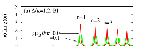
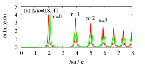
Figure 1: (color online) Imaginary part of the DSS $-\omega\,{\rm Im}\;\chi_{xx}(\omega)$ (in units of $\hbar^{2}/l^{2}$) with $\mu=0$ and $\Gamma/\kappa=0.02$ for (a) BI ($\Delta/\kappa=1.2$) and (b) TI ($\Delta/\kappa=0.8$). The parameters are $B=0.1$ T, $v=5.4\times 10^{5}$ m/s, and $\kappa=4.0$ meV assuming a silicene. There are regular peaks for both cases which stem from transitions between $-n$ and $n$ Landau levels with $|n|\geq 1$. In addition to those, an anomalous peak due to $n=0$ Landau levels appears at $\omega=2\kappa/\hbar$ (independent of the strength of the magnetic field) only for TI. When the Zeeman effect exists, e.g., $g\mu_{\rm B}B/\kappa=0.1$, the regular peaks split into two, while the anomalous peak shifts only to one direction.

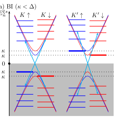
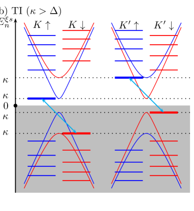
Figure 2: (color online) Landau level structures of Dirac fermions with alternating potential $\Delta$ and spin-orbit interactions $\kappa$ for (a) the BI ($|\kappa|<|\Delta|$) and (b) the TI ($|\kappa|>|\Delta|$) states. The two phases are characterized by the configurations of the $n=0$ Landau levels around the Fermi level ($\mu=0$). For the BI, the $n=0$ Landau levels have an opposite sign in each spin, so that the quantized Hall conductivity canceled out when the magnetic field is tuned off, and the absorption rate does not show the anomalous peak, because the transitions between $n=0$ Landau levels are not allowed.

Properties of DSS. Now let us consider the properties of DSS in these two phases of the Dirac system. The spin-spin correlation function is given in a Matsubara form as

$$\chi_{xx}(\tau)= -\braket{\mathcal{T}_{\tau}S^{x}(\tau)S^{x}(0)}_{0},$$ (11)

$$\chi_{xx}({\rm i}\nu_{m})= \frac{1}{\beta\hbar}\sum_{k,n}{\rm Tr}\;\mathcal{G}(\varepsilon_{k},{\rm i}\omega_{n})(\tau_{0}s_{x})\mathcal{G}(\varepsilon_{k},{\rm i}\omega_{n}^{+})(\tau_{0}s_{x}),$$ (12)

where $\Braket{\cdots}_{0}\equiv{\rm Tr}\;\cdots{\rm e}^{-\beta\mathcal{H}}/{\rm Tr}\;{\rm e}^{-\beta\mathcal{H}}$, with inverse temperature $\beta$. $\tau_{0}$ is the unit matrix, and the temperature Green’s function is given as $\mathcal{G}(\varepsilon,{\rm i}\omega_{n})=-({\rm i}\omega_{n}-(\varepsilon-\mu)/\hbar+{\rm i}\,{\rm sgn}(\omega_{n})\Gamma/\hbar)^{-1}$, $\omega_{n}^{+}\equiv\omega_{n}+\nu_{m}$ with $\omega_{n}$ and $\nu_{m}$ being Matsubara frequencies for fermions and bosons, respectively. The chemical potential and the impurity scattering time are denoted by $\mu(=0)$ and $\hbar/2\Gamma$, respectively. After analytic continuation ${\rm i}\nu_{m}\to\omega+{\rm i}0$, the retarded spin-spin correlation function is obtained as

$$\chi_{xx}(\omega)=\frac{\hbar^{2}}{8\pi l^{2}}\hbar\int_{-\infty}^{\infty}{\rm d}\Omega[-f^{\prime}(\hbar\Omega)]\sum_{\xi,s}\sum_{n,m}$$

$$\times\mathcal{X}(E_{n}^{\xi s},E_{m}^{\xi\bar{s}},\omega;\Omega)(A_{n}^{\xi s}A_{m}^{\xi\bar{s}}+B_{n}^{\xi s}B_{m}^{\xi\bar{s}})^{2}\delta_{|n|,|m|},$$ (13)

where $f(\varepsilon)=({\rm e}^{\beta(\varepsilon-\mu)}+1)^{-1}$ is the Fermi distribution function, $\bar{s}$ means the opposite spin of $s$, and $\mathcal{X}(x,y,\omega;\Omega)$ is defined as follows

$$\left.\frac{1}{\beta\hbar}\sum_{n}\frac{1}{({\rm i}\omega_{n}-x/\hbar)({\rm i}\omega_{n}^{+}-y/\hbar)}\right|_{{\rm i}\nu_{m}\to\omega}$$

$$=\hbar\int_{-\infty}^{\infty}{\rm d}\Omega[-f^{\prime}(\hbar\Omega)]\mathcal{X}(x,y,\omega;\Omega).$$ (14)

The transverse spin susceptibility is given by energy transitions between Landau levels labeled by the same absolute value of $n$ with opposite signs. This selection rule is much simpler than that in the current-current correlation function for the optical conductivity, which is related to the transitions between the $|n|$ and $|n\pm 1|$ Landau levels. Stille-T-N ; Tabert-N_2013L ; Tabert-N_2013B1 ; Tabert-N_2013B2

Now we turn our attention only to the imaginary part of the DSS multiplied by the frequency $-\omega\,{\rm Im}\;\chi_{xx}(\omega)$, which is experimentally observable as discussed later. The real part can also be obtained via the Kramers-Kronig relation. As shown in Fig. 1, $-\omega\,{\rm Im}\;\chi_{xx}(\omega)$ at $\mu=0$ has several peaks corresponding to the transitions between the Landau levels below and above the Fermi level with the same absolute values of the index $|n|\geq 1$. We also find that an anomalous peak appears only for the TI region ($|\kappa|>|\Delta|$), whose resonant frequency is independent of the strength of the magnetic field. Actually, for the clean and zero temperature limit ($\Gamma\to 0$ and $T\to 0$), we get the following $\delta$-function peaks,

$$-{\rm Im}\;\chi_{xx}(\omega)=\frac{\hbar^{2}}{4l^{2}}\biggl{[}\sum_{n=1}^{\infty}2(A_{n}^{+1,\uparrow}B_{n}^{+1,\downarrow}-B_{n}^{+1,\uparrow}A_{n}^{+1,\downarrow})^{2}$$

$$\times\delta(\omega-(E_{n}^{+1,\uparrow}+E_{n}^{+1,\downarrow})/\hbar)+\theta(\kappa^{2}-\Delta^{2})\delta(\omega-2|\kappa|/\hbar)\biggr{]}.$$ (15)

The last term of Eq. (15) is the anomalous peak at $\omega=2\kappa/\hbar$ which stems from the transition between the $n=0$ Landau levels with opposite spins. This peak can be observed only in the TI where one of the two levels is below the Fermi level, as shown in Fig. 2. Physically, this peak is related to an energy $2\kappa$ to make an edge state with the spin current in the opposite direction via spin flipping. Therefore, we can identify whether the system is a TI or a BI, by observing this anomalous peak. The numerical value of the frequency of the anomalous peaks is estimated as $\omega\approx 12$ THz for silicene with $\kappa=4.0$ meV. Tsai

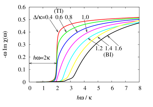
Figure 3: (color online) Imaginary part of the DSS, $-\omega\,{\rm Im}\;\chi_{xx}(\omega)$ (in unit of $\kappa^{2}/v^{2}$), with $B=0$ and $\Gamma/\kappa=0.02$ for several values of $\Delta/\kappa=0.4$-$1.6$. For small $\Gamma$, $-\omega\,{\rm Im}\;\chi_{xx}(\omega)$ is discontinuous (continuous) function at the threshold frequency $\omega_{\rm c}=2\kappa/\hbar$ ($\omega_{\rm c}=2\Delta/\hbar$) for TI (BI).

We can also show that the anomalous peak can easily be distinguished from the regular peaks, even if the Zeeman effect is taken into account. In the presence of the Zeeman effect, Eq. (13) is modified as $\mathcal{X}(E_{n}^{\xi s},E_{m}^{\xi\bar{s}},\omega;\Omega)$ $\to$ $\mathcal{X}(E_{n}^{\xi s}+sg\mu_{\rm B}B/2,E_{m}^{\xi\bar{s}}+\bar{s}g\mu_{\rm B}B/2,\omega;\Omega)$. As shown in Fig. 1, the regular peaks split into two parts $\Delta\omega=\pm\mu_{\rm B}B/\hbar$, while the anomalous peak shifts to one direction $\Delta\omega={\rm sgn}(\kappa)\mu_{\rm B}B/\hbar$. This is because the valley degeneracy is lifted by the Zeeman effect for $|n|\geq 1$ Landau levels, while the Landau levels are uniformly shifted for $n=0$. Therefore, the DSS is still effective information to characterize the TI in the presence of the Zeeman coupling, if it is sufficiently smaller than the spin-orbit coupling, as usually expected for TIs. Furthermore the Zeeman shift of the anomalous peak has information to identify the sign of the spin-orbit coupling $\kappa$.

Case without static magnetic field. So far we have assumed the Landau quantization by a static magnetic field in a bulk system, so that the peak structures of ${\rm Im}\;\chi_{xx}(\omega)$ vanish in the $B=0$ cases, and it becomes a continuous function of $\omega$. However, as shown in Fig. 3, the threshold value of the frequency $\omega_{\rm c}$ which gives the minimum edge of finite $-\omega\,{\rm Im}\;\chi_{xx}(\omega)$ is $\omega_{\rm c}=2\Delta/\hbar$ for the BI and $\omega_{\rm c}=2\kappa/\hbar$ for the TI. This difference can be easily understood from Eq. (15) for $B\to 0$ which gives $\hbar\omega_{\rm c}=|\Delta_{+1,\uparrow}|+|\Delta_{+1,\downarrow}|$. The line shape of ${\rm Im}\;\chi_{xx}(\omega)$ is also different for the two phases: ${\rm Im}\;\chi_{xx}(\omega)$ grows continuously from $0$ for the BI while it grows discontinuously for the TI. This can also be understood by examining the $B\to 0$ limit of Eq. (15): For $|\Delta|\gg|\kappa|$, we get $-{\rm Im}\;\chi_{xx}(2\Delta/\hbar)=0$ and $\lim_{\omega\to\infty}[-\omega\>{\rm Im}\;\chi_{xx}(\omega)]=\frac{\kappa^{2}}{4v^{2}}$, while for $|\Delta|\ll|\kappa|$, we have $-{\rm Im}\;\chi_{xx}(2\kappa/\hbar)=\frac{\hbar\kappa}{4v^{2}}$ and $\lim_{\omega\to\infty}[-\omega\>{\rm Im}\;\chi_{xx}(\omega)]=\frac{2\kappa^{2}-\Delta^{2}}{4v^{2}}$. These features may also give supplemental information to distinguish a TI and a BI.

Possible experiments. Finally, let us consider how we observe ${\rm Im}\;\chi_{xx}(\omega)$ in real experiments. For an example, we examine a 2D electron system with a static magnetic field and a transverse ac magnetic field. The Hamiltonian of the system is expressed as

$$\mathcal{H}(t)=\mathcal{H}+V(t),$$ (16)

where $\mathcal{H}$ and $V(t)$ are the time-independent and time-dependent parts of the Hamiltonian, respectively. For the static and the dynamic magnetic fields,

$$\bm{B}(t)=\bm{B}+\bm{B}_{\rm R}\cos(\omega t),$$ (17)

with $\bm{B}=(0,0,B)$ and $\bm{B}_{\rm R}=(B_{\rm R},0,0)$, we may choose the vector potential as $\bm{A}=B(-y/2,x/2,0)$, $\bm{A}_{\rm R}=B_{\rm R}(0,0,y)$. In order to discuss general situations, we first consider a “non-relativistic” system with a parabolic band, and with an electron mass $m$. Then Eq. (16) is given by

$$\mathcal{H}= \mathcal{H}_{0}(\bm{A})+g\mu_{\rm B}B\int{\rm d}\bm{r}S^{z}(\bm{r}),$$ (18)

$$V(t)= g\mu_{\rm B}B_{\rm R}\cos(\omega t)\int{\rm d}\bm{r}S^{x}(\bm{r})$$

$$-\frac{\cos^{2}(\omega t)}{2c}\int{\rm d}\bm{r}\bm{A}_{\rm R}(\bm{r})\cdot\bm{J}_{\rm d}(\bm{r}),$$ (19)

where $S^{\alpha}\equiv\int{\rm d}\bm{r}\hat{\psi}_{s}^{{\dagger}}s^{\alpha}_{ss^{\prime}}\hat{\psi}_{s^{\prime}}^{\mathstrut}$ with an electron operator $\hat{\psi}_{s}$. $\bm{J}_{\rm d}\equiv-\frac{e^{2}}{mc}\bm{A}_{\rm R}\hat{\psi}_{s}^{\dagger}\hat{\psi}_{s}^{\mathstrut}$ means a diamagnetic current induced by the dynamic magnetic field, whereas a paramagnetic current $\bm{J}_{\rm p}\equiv-\frac{e\hbar}{2m{\rm i}}\{\hat{\psi}^{\dagger}_{s}\nabla\hat{\psi}_{s}^{\mathstrut}-[\nabla\hat{\psi}^{\dagger}_{s}(\bm{r})]\hat{\psi}^{\mathstrut}_{s}\}$ is included in $\mathcal{H}_{0}$. We have also used the relation $\bm{A}_{\rm R}(\bm{r})\cdot\bm{J}_{\rm p}(\bm{r})=0$, which is satisfied in 2D systems.

Then the absorption rate of the dynamic magnetic field is obtained up to the second order of $V$ as

$$I(\omega) =\int_{0}^{T}\frac{{\rm d}t^{\prime}}{T}\frac{{\rm d}}{{\rm d}t^{\prime}}{\rm Tr}\;[\rho(t^{\prime})\mathcal{H}(t^{\prime})]$$ (20)

$$\approx-\frac{(g\mu_{\rm B}B_{\rm R})^{2}\omega}{2\hbar}{\rm Im}\;\chi_{xx}^{\rm R}(\omega),$$ (21)

where $T\equiv 2\pi/\omega$, $\rho$ is a density matrix of Eq. (16), and $\chi_{xx}^{\rm R}(\omega)$ is the Fourier transform of the retarded transverse spin-spin correlation function,

$$\chi_{xx}^{\rm R}(t)=-{\rm i}\theta(t)\Braket{\left[S_{\rm tot}^{x}(t),S_{\rm tot}^{x}(0)\right]}_{0}.$$ (22)

Here, we should note that the orbital contributions of the ac field do not appear in Eq. (21), because $\bm{A}_{\rm R}(\bm{r})\cdot\bm{J}_{\rm d}(\bm{r})$ is canceled in the time integral, and $I(\omega)$ becomes just the same form as a usual ESR formula for localized spin systems. Kubo-T This situation is realized only in 2D systems where the electrons do not have a path to move along the $z$ direction. In Dirac systems, the current operator does not have a diamagnetic part because of the linear dispersion relation, so that the last term of the right hand side of Eq. (19) does not exist. Thus Eq. (21) can also be applied to current 2D Dirac systems.

Summary. We have discussed the dynamic transverse spin susceptibility (DSS) of a 2D Dirac system with a spin-orbit interaction $\kappa$ and an alternating potential $\Delta$ (2). Its imaginary part is related to the absorption rate in response to a transverse ac magnetic field. When a static magnetic field is applied to the system, the imaginary part of the DSS shows an anomalous peak at frequency $\omega=2\kappa/\hbar$ for the TI. This is related to an energy to make an edge state with the spin current in the opposite direction via spin flipping. On the other hand, when the static magnetic field is turned off, the imaginary part of the DSS becomes a continuous function of $\omega$ with different values of threshold frequencies, $\omega_{\rm c}=2\kappa/\hbar$ for the TI and $\omega_{\rm c}=2\Delta/\hbar$ for the BI, respectively. These properties enable us to identify the TI directly only from the bulk information, without observing a topological transition from the BI. The DSS is considered to be a relevant probe for TIs in more general cases. However, in the case of the BHZ modelBernevig-H-Z which describes a TI realized in HgTe quantum wells, the present theory cannot be applied straightforwardly, since the $n=0$ Landau levels depend on the strength of the magnetic fieldKonig-2007 . We also need extended discussions for the original Kane-Mele model including the Rashba interactionsKane-M where the $z$-component of spins is not conserved.

The authors thank S. C. Furuya, Y. Kubo, and N. Hatano for helpful discussions. M. N. thanks the Max Planck Institute for Solid State Research where a part of this work has been done.

References

- (1) C. L. Kane and E. J. Mele, Phys. Rev. Lett. 95, 146802 (2005).
- (2) M. König, S. Wiedmann, C. Brune, A. Roth, H. Buhmann, L. W. Molenkamp, X.-L. Qi, and S.-C. Zhang, Science, 318, 766 (2007).
- (3) M. König, H. Buhmann, L. W. Molenkamp, T. Hughes, C.-X. Liu, X.-L. Qi, and S.-C. Zhang, J. Phys. Soc. Jpn., 77, 031007 (2008).
- (4) A. Roth, C. Bruene, H. Buhmann, L. W. Molenkamp, J. Maciejko, X.-L. Qi, and S.-C. Zhang, Science, 325, 294 (2009).
- (5) B. A. Bernevig, T. L. Hughes, and S. C. Zhang, Science 314, 1757 (2006).
- (6) B. Lalmi, H. Oughaddou, H. Enriquez, A. Kara, S. Vizzini, B. Ealet, and B. Aufray, Appl. Phys. Lett. 97, 223109 (2010).
- (7) P. De Padova, C. Quaresima, C. Ottaviani, P. M. Sheverdyaeva, P. Moras, C. Carbone, D. Topwal, B. Olivieri, A. Kara, H. Oughaddou, B. Aufray, and G. Le Lay, Appl. Phys. Lett. 96, 261905 (2010).
- (8) P. De Padova, C. Quaresima, B. Olivieri, P. Perfetti, and G. Le Lay, Appl. Phys. Lett. 98, 081909 (2011).
- (9) P. Vogt, P. De Padova, C. Quaresima, J. Avila, E. Frantzeskakis, M. C. Asensio, A. Resta, B. Ealet, and G. Le Lay, Phys. Rev. Lett. 108, 155501 (2012).
- (10) C.-L. Lin, R. Arafune, K. Kawahara, N. Tsukahara, E. Minamitani, Y. Kim, N. Takagi, and M. Kawai, Appl. Phys. Express 5, 045802 (2012).
- (11) A. Fleurence, R. Friedlein, T. Ozaki, H. Kawai, Y. Wang, and Y. Yamada-Takamura, Phys. Rev. Lett. 108, 245501 (2012).
- (12) C.-C. Liu, W. Feng, and Y. Yao, Phys. Rev. Lett. 107, 076802 (2011).
- (13) C.-C. Liu, H. Jiang, and Y. Yao, Phys. Rev. B 84, 195430 (2011).
- (14) K. F. Mak, C. Lee, J. Hone, J. Shan, and T. F. Heinz, Phys. Rev. Lett. 105, 136805 (2010).
- (15) D. Xiao, G.-B. Liu, W. Feng, X. Xu, and W. Yao, Phys. Rev. Lett. 108, 196802 (2012).
- (16) M. Ezawa, Phys. Rev. B 86, 161407(R) (2012).
- (17) L. Stille, C. J. Tabert, and E. J. Nicol Phys. Rev. B 86, 195405 (2012).
- (18) C. J. Tabert and E. J. Nicol, Phys. Rev. Lett. 110, 197402 (2013).
- (19) C. J. Tabert and E. J. Nicol Phys. Rev. B 88, 085434 (2013)
- (20) A. Dyrdal and J. Barnaś, Phys. Status Solidi RRL 6, 340 (2012).
- (21) M. Tahir, A. Manchon, K. Sabeeh, and U. Schwingenschlögl, Appl. Phys. Lett. 102, 162412 (2013).
- (22) C. J. Tabert and E. J. Nicol Phys. Rev. B 87, 235426 (2013)
- (23) C. J. Tabert and E. J. Nicol Phys. Rev. B 89, 195410 (2014).
- (24) H.-R. Chang, J. Zhou, H. Zhang, and Y. Yao, Phys. Rev. B 89, 201411 (2014).
- (25) B. Van Duppen, P. Vasilopoulos, and F. M. Peeters, Phys. Rev. B 90, 035142 (2014).
- (26) V. P. Gusynin, S. G. Sharapov, and A. A. Varlamov, Phys. Rev. B 90, 155107 (2014).
- (27) S. K. Islam and T. K. Ghosh, J. Phys.: Condens. Matter 26, 335303 (2014).
- (28) V. Y. Tsaran and S. G. Sharapov, Phys. Rev. B 90, 205417 (2014).
- (29) K. Shakouri, P. Vasilopoulos, V. Vargiamidis, and F. M. Peeters, Phys. Rev. B 90, 125444 (2014).
- (30) C. J. Tabert, J. P. Carbotte, and E. J. Nicol, Phys. Rev. B 91, 035423 (2015).
- (31) A. Raoux, F. Piechon, J. N. Fuchs, and G. Montambaux, Phys. Rev. B 91, 085120 (2015).
- (32) F. D. M. Haldane, Phys. Rev. Lett. 61, 2015 (1988).
- (33) W.-F. Tsai, C.-Y. Huang, T.-R. Chang, H. Lin, H.-T. Jeng, and A. Bansil, Nat. Commun. 4, 1500 (2013).
- (34) R. Kubo and K. Tomita, J. Phys. Soc. Jpn. 9, 888 (1954).