Relating transverse structure of various parton distributions

Tanmay Maji1, Chandan Mondal1, D. Chakrabarti1 and O. V. Teryaev2,3 1Department of Physics, Indian Institute of Technology Kanpur, Kanpur 208016, India
2Bogoliubov Laboratory of Theoretical Physics, Joint Institute of Nuclear Research, 141980 Dubna, Russia
3 National Research Nuclear University "MEPhI"(Moscow Engineering Physics Institute), Kashirskoe highway 31, 115409 Moscow, Russia
Abstract

We present the results of T-even TMDs in a light front quark-diquark model of nucleons with the wave functions constructed from the soft-wall AdS/QCD prediction. The relations amongst TMDs are discussed. The psubscript𝑝perpendicular-top_{\perp} dependence of the TMDs are compared with the t𝑡t-dependence of the GPDs and the relation between the respective dependencies are found..

pacs:
14.20.Dh,12.39.-x,13.60.-r,12.38.Aw

I Introduction

The three dimensional picture of proton is one of the most interesting and challenging tasks in particle physics. Recently, there are many theoretical investigations as well as experiments (e.g. ZEUS, COMPASS, HERMES, CLAS expts ) to understand the generalized parton distributions(GPDs) and transverse momentum dependent(TMDs) distributions which encode these informations. These objects represent similar albeit non-identical transverse structure and in this paper we are aiming to relate these in a straightforward manner. For that purpose we use a light front quark-scalar diquark model of proton where the wave functions are constructed from AdS/QCDBT1 predictions, and present a unified description of the TMDs and GPDs and the relations between these two different distribution functions.

The TMDs (see collins and references therein) are required to describe the Semi-Inclusive Deep Inelastic Scattering(SIDIS) or Drell-Yan processes, whereas GPDs (see diehl and references therein) are required for exclusive processes like deeply virtual Compton scattering or vector meson productions. Three of the TMDs, f1(x,p),g1L(x,p),h1(x,p)subscript𝑓1𝑥subscript𝑝perpendicular-tosubscript𝑔1𝐿𝑥subscript𝑝perpendicular-tosubscript1𝑥subscript𝑝perpendicular-tof_{1}(x,p_{\perp}),~{}g_{1L}(x,p_{\perp}),~{}h_{1}(x,p_{\perp}) are generalization of the three PDFs, the unpolarized distribution f1(x)subscript𝑓1𝑥f_{1}(x), helicity distribution function g1(x)subscript𝑔1𝑥g_{1}(x) and the transversity distribution h1(x)subscript1𝑥h_{1}(x). Other TMDs do not have simple collinear limit. Both, TMDs and GPDs are studied in several QCD inspired models. In this paper, we mainly concentrate on the relations among the TMDs and the relations between TMDs and the GPDs and their moments.

TMDs have been investigated in several QCD inspired models, e.g., in a diquark spectator model Mulders ; Bacchetta , in MIT bag modelbag , in a covariant parton modelparton . The relations between the TMDs and PDFs were studied inefremov and the relations with GPDs were studied in detail in meissner . Some relations between the TMDs and GPDs were also observed in muller .

These relations are model dependent and it is not guaranteed that they should hold in QCD. A model independent derivation of the relations is not yet possible. Nevertheless, from phenomenological point of view, these relations may provide additional constraints on model predictions. Here, we demonstrate a novel relation between the TMDs and the GPDs which relates the t𝑡t( square of momentum transferred) dependence of GPDs with the p2superscriptsubscript𝑝perpendicular-to2p_{\perp}^{2} dependence of TMDs. This may reflect the sort of Veneziano-like st𝑠𝑡s\leftrightarrow t duality (see Teryaev:2015tza . Sect.4). The p2superscriptsubscript𝑝perpendicular-to2p_{\perp}^{2} dependence in TMDs coming form AdS/QCD wavefunction explains why the TMDs in lattice calculations show approximate x𝑥x and p2superscriptsubscript𝑝perpendicular-to2p_{\perp}^{2} factorization. The same factorization is also used in phenomenological models of TMDs.

II light-front diquark Model

In this model we assume that the incoming photon, carrying a high momentum, interacts with one of the valence quark inside the nucleon and other two valence quarks form a bound state of spin-0 (scalar diquark). Therefore the nucleon state |P,Sket𝑃𝑆|P,S\rangle having momentum P and spin S, can be represented as 2-particle Fock-state. In this paper we consider the scalar diquark model Gut .

The light-cone components of quark momentum p𝑝p and spectator momentum PXsubscript𝑃𝑋P_{X} are

p𝑝\displaystyle p \displaystyle\equiv (xP+,p2+|p|2xP+,p),𝑥superscript𝑃superscript𝑝2superscriptsubscriptpperpendicular-to2𝑥superscript𝑃subscriptpperpendicular-to\displaystyle\bigg{(}xP^{+},\frac{p^{2}+|\textbf{p}_{\perp}|^{2}}{xP^{+}},\textbf{p}_{\perp}\bigg{)}, (1)
PXsubscript𝑃𝑋\displaystyle P_{X} \displaystyle\equiv ((1x)P+,PX,p).1𝑥superscript𝑃superscriptsubscript𝑃𝑋subscriptpperpendicular-to\displaystyle\bigg{(}(1-x)P^{+},P_{X}^{-},-\textbf{p}_{\perp}\bigg{)}. (2)

The 2-particle Fock-state expansion for Jz=±12superscript𝐽𝑧plus-or-minus12J^{z}=\pm\frac{1}{2} are given by

|P;±ket𝑃plus-or-minus\displaystyle|P;\pm\rangle =\displaystyle= qdxd2p2(2π)3x(1x)[\displaystyle\sum_{q}\int\frac{dx~{}d^{2}\textbf{p}_{\perp}}{2(2\pi)^{3}\sqrt{x(1-x)}}\bigg{[} (3)
ψ+q±(x,p)|+12,0;xP+,p+limit-fromsubscriptsuperscript𝜓limit-from𝑞plus-or-minus𝑥subscriptpperpendicular-toket120𝑥superscript𝑃subscriptpperpendicular-to\displaystyle\psi^{q\pm}_{+}(x,\textbf{p}_{\perp})|+\frac{1}{2},0;xP^{+},\textbf{p}_{\perp}\rangle+
ψq±(x,p)|12,0;xP+,p],\displaystyle\psi^{q\pm}_{-}(x,\textbf{p}_{\perp})|-\frac{1}{2},0;xP^{+},\textbf{p}_{\perp}\rangle\bigg{]},

where the |λq,λs;xP+,pketsubscript𝜆𝑞subscript𝜆𝑠𝑥superscript𝑃subscriptpperpendicular-to|\lambda_{q},\lambda_{s};xP^{+},\textbf{p}_{\perp}\rangle represents a two particle state with a quark of spin λq=±12subscript𝜆𝑞plus-or-minus12\lambda_{q}=\pm\frac{1}{2}, momentum p𝑝p and a scalar spectator(λs=0subscript𝜆𝑠0\lambda_{s}=0). The states are normalized as:

λq,λs;xP+,p\displaystyle\langle\lambda^{\prime}_{q},\lambda^{\prime}_{s};x^{\prime}P^{+},\textbf{p}^{\prime}_{\perp} \displaystyle\mid λq,λs;xP+,p=\displaystyle\!\lambda_{q},\lambda_{s};xP^{+},\textbf{p}_{\perp}\rangle=
i=1216π3pi+subscriptsuperscriptproduct2𝑖116superscript𝜋3subscriptsuperscript𝑝𝑖\displaystyle\prod^{2}_{i=1}16\pi^{3}p^{+}_{i} δ(pi+pi+)δ2(pipi)δλiλi.𝛿subscriptsuperscript𝑝𝑖subscriptsuperscript𝑝𝑖superscript𝛿2subscriptsuperscriptpperpendicular-toabsent𝑖subscriptpperpendicular-toabsent𝑖subscript𝛿subscriptsuperscript𝜆𝑖subscript𝜆𝑖\displaystyle\!\!\!\!\!\!\!\delta(p^{\prime+}_{i}-p^{+}_{i})\delta^{2}(\textbf{p}^{\prime}_{\perp i}-\textbf{p}_{\perp i})\delta_{\lambda^{\prime}_{i}\lambda_{i}}. (4)

ψλqqλNsubscriptsuperscript𝜓𝑞subscript𝜆𝑁subscript𝜆𝑞\psi^{q\lambda_{N}}_{\lambda_{q}} are the light-front wave functions with nucleon helicities λN=±subscript𝜆𝑁plus-or-minus\lambda_{N}=\pm.We adopt the generic ansatz for the quark-diquark model of the valence Fock state of the nucleon LFWFs at a scale μ0=313subscript𝜇0313\mu_{0}=313 MeV as proposed in Gut :

ψ+q+(x,p)subscriptsuperscript𝜓limit-from𝑞𝑥subscriptpperpendicular-to\displaystyle\psi^{q+}_{+}(x,\textbf{p}_{\perp}) =\displaystyle= φq(1)(x,p),superscript𝜑𝑞1𝑥subscriptpperpendicular-to\displaystyle\varphi^{q(1)}(x,\textbf{p}_{\perp}),
ψq+(x,p)subscriptsuperscript𝜓limit-from𝑞𝑥subscriptpperpendicular-to\displaystyle\psi^{q+}_{-}(x,\textbf{p}_{\perp}) =\displaystyle= p1+ip2xMφq(2)(x,p),superscript𝑝1𝑖superscript𝑝2𝑥𝑀superscript𝜑𝑞2𝑥subscriptpperpendicular-to\displaystyle-\frac{p^{1}+ip^{2}}{xM}\varphi^{q(2)}(x,\textbf{p}_{\perp}),
ψ+q(x,p)subscriptsuperscript𝜓limit-from𝑞𝑥subscriptpperpendicular-to\displaystyle\psi^{q-}_{+}(x,\textbf{p}_{\perp}) =\displaystyle= p1ip2xMφq(2)(x,p),superscript𝑝1𝑖superscript𝑝2𝑥𝑀superscript𝜑𝑞2𝑥subscriptpperpendicular-to\displaystyle\frac{p^{1}-ip^{2}}{xM}\varphi^{q(2)}(x,\textbf{p}_{\perp}), (5)
ψq(x,p)subscriptsuperscript𝜓limit-from𝑞𝑥subscriptpperpendicular-to\displaystyle\psi^{q-}_{-}(x,\textbf{p}_{\perp}) =\displaystyle= φq(1)(x,p),superscript𝜑𝑞1𝑥subscriptpperpendicular-to\displaystyle\varphi^{q(1)}(x,\textbf{p}_{\perp}),

where φq(1)(x,p)superscriptsubscript𝜑𝑞1𝑥subscriptpperpendicular-to\varphi_{q}^{(1)}(x,\textbf{p}_{\perp}) and φq(2)(x,p)superscriptsubscript𝜑𝑞2𝑥subscriptpperpendicular-to\varphi_{q}^{(2)}(x,\textbf{p}_{\perp}) are the wave functions predicted by soft-wall AdS/QCD

φq(i)(x,p)superscript𝜑𝑞𝑖𝑥subscriptpperpendicular-to\displaystyle\varphi^{q(i)}(x,\textbf{p}_{\perp}) =\displaystyle= Nq(i)4πκlog(1/x)1xxaq(i)(1x)bq(i)superscriptsubscript𝑁𝑞𝑖4𝜋𝜅1𝑥1𝑥superscript𝑥superscriptsubscript𝑎𝑞𝑖superscript1𝑥superscriptsubscript𝑏𝑞𝑖\displaystyle N_{q}^{(i)}\frac{4\pi}{\kappa}\sqrt{\frac{\log(1/x)}{1-x}}x^{a_{q}^{(i)}}(1-x)^{b_{q}^{(i)}} (6)
exp[p22κ2log(1/x)(1x)2],superscriptsubscriptpperpendicular-to22superscript𝜅21𝑥superscript1𝑥2\displaystyle\exp\bigg{[}-\frac{\textbf{p}_{\perp}^{2}}{2\kappa^{2}}\frac{\log(1/x)}{(1-x)^{2}}\bigg{]},

where κ=0.4𝜅0.4\kappa=0.4 GeV CM1 is the AdS/QCD scale parameter. The values of the parameters aq(i)subscriptsuperscript𝑎𝑖𝑞a^{(i)}_{q} and bq(i)subscriptsuperscript𝑏𝑖𝑞b^{(i)}_{q} and the constants Nq(i)subscriptsuperscript𝑁𝑖𝑞N^{(i)}_{q} were fixed by fitting the nucleon form factors. For κ=0.4𝜅0.4\kappa=0.4 GeV, the parameters areChi au(1)=0.02,au(2)=1.05,bu(1)=0.022,bu(2)=0.15,Nu(1)=2.055,Nu(2)=1.322,ad(1)=0.1,ad(2)=1.07,bd(1)=0.38,bd(2)=0.2,Nd(1)=1.7618,&Nd(2)=2.4827.formulae-sequencesubscriptsuperscript𝑎1𝑢0.02formulae-sequencesubscriptsuperscript𝑎2𝑢1.05formulae-sequencesubscriptsuperscript𝑏1𝑢0.022formulae-sequencesubscriptsuperscript𝑏2𝑢0.15formulae-sequencesubscriptsuperscript𝑁1𝑢2.055formulae-sequencesubscriptsuperscript𝑁2𝑢1.322formulae-sequencesubscriptsuperscript𝑎1𝑑0.1formulae-sequencesubscriptsuperscript𝑎2𝑑1.07formulae-sequencesubscriptsuperscript𝑏1𝑑0.38formulae-sequencesubscriptsuperscript𝑏2𝑑0.2formulae-sequencesubscriptsuperscript𝑁1𝑑1.7618subscriptsuperscript𝑁2𝑑2.4827a^{(1)}_{u}=0.02,~{}a^{(2)}_{u}=1.05,~{}b^{(1)}_{u}=0.022,~{}b^{(2)}_{u}=-0.15,N^{(1)}_{u}=2.055,N^{(2)}_{u}=1.322,~{}a^{(1)}_{d}=0.1,~{}a^{(2)}_{d}=1.07,~{}b^{(1)}_{d}=0.38,~{}b^{(2)}_{d}=-0.2,~{}N^{(1)}_{d}=1.7618,~{}\&~{}N^{(2)}_{d}=-2.4827. For aq(i)=bq(i)=0superscriptsubscript𝑎𝑞𝑖superscriptsubscript𝑏𝑞𝑖0a_{q}^{(i)}=b_{q}^{(i)}=0, the wave functions reduce to the AdS/QCD predictionBT .

A transversely polarized nucleon with polarization S^T=(cosϕS,sinϕS)subscript^𝑆𝑇subscriptitalic-ϕ𝑆subscriptitalic-ϕ𝑆\hat{S}_{T}=(\cos\phi_{S},\sin\phi_{S}) in the transverse plane can be written as

P;ST=12(|P;++eiϕS|P;)ket𝑃subscript𝑆𝑇12ket𝑃superscript𝑒𝑖subscriptitalic-ϕ𝑆ket𝑃\mid P;S_{T}\rangle=\frac{1}{\sqrt{2}}\bigg{(}|P;+\rangle+e^{i\phi_{S}}|P;-\rangle\bigg{)} (7)

Without loss of generality, we choose the nucleon polarization along x𝑥x axis i.e., ϕS=0subscriptitalic-ϕ𝑆0\phi_{S}=0.

III TMDs

The unintegrated quark-quark correlator for polarized SIDIS is defined as

Φq[Γ](x,p;S)superscriptΦ𝑞delimited-[]Γ𝑥subscriptpperpendicular-to𝑆\displaystyle\Phi^{q[\Gamma]}(x,\textbf{p}_{\perp};S) =\displaystyle= 14dz(2π)d2zT(2π)2eip.z14𝑑superscript𝑧2𝜋superscript𝑑2subscript𝑧𝑇superscript2𝜋2superscript𝑒formulae-sequence𝑖𝑝𝑧\displaystyle\frac{1}{4}\int\frac{dz^{-}}{(2\pi)}\frac{d^{2}z_{T}}{(2\pi)^{2}}e^{ip.z} (8)
P;S|ψ¯q(0)Γ𝒲[0,z]ψq(z)|P;S,quantum-operator-product𝑃𝑆superscript¯𝜓𝑞0Γsubscript𝒲0𝑧superscript𝜓𝑞𝑧𝑃𝑆\displaystyle\!\!\!\!\!\langle P;S|\overline{\psi}^{q}(0)\Gamma\mathcal{W}_{[0,z]}\psi^{q}(z)|P;S\rangle,

for a quark q. The summations over the color indices of quarks are implied. Here p𝑝p is the momentum of the struck quark inside the nucleon having momentum P, helicity S and x(x=p+/P+)𝑥𝑥superscript𝑝superscript𝑃x~{}(x=p^{+}/P^{+}) is the longitudinal momentum fraction carried by struck quark. We choose the lightcone gauge A+=0superscript𝐴0A^{+}=0 and a frame where the nucleon momentum and quark momentum are P(P+,M2P+,0),q(xBP+,Q2xBP+,0)formulae-sequence𝑃superscript𝑃superscript𝑀2superscript𝑃0𝑞subscript𝑥𝐵superscript𝑃superscript𝑄2subscript𝑥𝐵superscript𝑃0P\equiv(P^{+},\frac{M^{2}}{P^{+}},\textbf{0}),~{}q\equiv(x_{B}P^{+},\frac{Q^{2}}{x_{B}P^{+}},\textbf{0}) respectively, xB=Q22P.qsubscript𝑥𝐵superscript𝑄2formulae-sequence2𝑃𝑞x_{B}=\frac{Q^{2}}{2P.q} is the Bjorken Scaling with Q2=q2superscript𝑄2superscript𝑞2Q^{2}=-q^{2}. The nucleon with helicity λ𝜆\lambda has spin components S+=λP+M,S=λPM,formulae-sequencesuperscript𝑆𝜆superscript𝑃𝑀superscript𝑆𝜆superscript𝑃𝑀S^{+}=\lambda\frac{P^{+}}{M},~{}S^{-}=\lambda\frac{P^{-}}{M}, and STsubscript𝑆𝑇S_{T}. In leading twist, the TMDs are defined as

Φq[γ+](x,p;S)superscriptΦ𝑞delimited-[]superscript𝛾𝑥subscriptpperpendicular-to𝑆\displaystyle\Phi^{q[\gamma^{+}]}(x,\textbf{p}_{\perp};S) =\displaystyle= f1q(x,p2)ϵTijpiSTjMf1Tq(x,p2),superscriptsubscript𝑓1𝑞𝑥superscriptsubscriptpperpendicular-to2subscriptsuperscriptitalic-ϵ𝑖𝑗𝑇subscriptsuperscript𝑝𝑖perpendicular-tosubscriptsuperscript𝑆𝑗𝑇𝑀subscriptsuperscript𝑓perpendicular-toabsent𝑞1𝑇𝑥superscriptsubscriptpperpendicular-to2\displaystyle f_{1}^{q}(x,\textbf{p}_{\perp}^{2})-\frac{\epsilon^{ij}_{T}p^{i}_{\perp}S^{j}_{T}}{M}f^{\perp q}_{1T}(x,\textbf{p}_{\perp}^{2}),
Φq[γ+γ5](x,p;S)superscriptΦ𝑞delimited-[]superscript𝛾superscript𝛾5𝑥subscriptpperpendicular-to𝑆\displaystyle\Phi^{q[\gamma^{+}\gamma^{5}]}(x,\textbf{p}_{\perp};S) =\displaystyle= λg1Lq(x,p2)+p.STMg1Tq(x,p2),𝜆superscriptsubscript𝑔1𝐿𝑞𝑥superscriptsubscriptpperpendicular-to2formulae-sequencesubscriptpperpendicular-tosubscriptS𝑇𝑀subscriptsuperscript𝑔𝑞1𝑇𝑥superscriptsubscriptpperpendicular-to2\displaystyle\lambda g_{1L}^{q}(x,\textbf{p}_{\perp}^{2})+\frac{\textbf{p}_{\perp}.\textbf{S}_{T}}{M}g^{q}_{1T}(x,\textbf{p}_{\perp}^{2}),
Φq[iσj+γ5](x,p;S)superscriptΦ𝑞delimited-[]𝑖superscript𝜎limit-from𝑗superscript𝛾5𝑥subscriptpperpendicular-to𝑆\displaystyle\Phi^{q[i\sigma^{j+}\gamma^{5}]}(x,\textbf{p}_{\perp};S) =\displaystyle= STjh1q(x,p2)+λpjMh1Lq(x,p2)subscriptsuperscript𝑆𝑗𝑇superscriptsubscript1𝑞𝑥superscriptsubscriptpperpendicular-to2𝜆subscriptsuperscript𝑝𝑗perpendicular-to𝑀subscriptsuperscriptperpendicular-toabsent𝑞1𝐿𝑥superscriptsubscriptpperpendicular-to2\displaystyle S^{j}_{T}h_{1}^{q}(x,\textbf{p}_{\perp}^{2})+\lambda\frac{p^{j}_{\perp}}{M}h^{\perp q}_{1L}(x,\textbf{p}_{\perp}^{2}) (9)
+\displaystyle+ 2pjp.STSTjp22M2h1Tq(x,p2)formulae-sequence2subscriptsuperscript𝑝𝑗perpendicular-tosubscriptpperpendicular-tosubscriptS𝑇subscriptsuperscript𝑆𝑗𝑇subscriptsuperscriptp2perpendicular-to2superscript𝑀2subscriptsuperscriptperpendicular-toabsent𝑞1𝑇𝑥superscriptsubscriptpperpendicular-to2\displaystyle\frac{2p^{j}_{\perp}\textbf{p}_{\perp}.\textbf{S}_{T}-S^{j}_{T}\textbf{p}^{2}_{\perp}}{2M^{2}}h^{\perp q}_{1T}(x,\textbf{p}_{\perp}^{2})
\displaystyle- ϵTijpiMh1q(x,p2).superscriptsubscriptitalic-ϵ𝑇𝑖𝑗subscriptsuperscript𝑝𝑖perpendicular-to𝑀subscriptsuperscriptperpendicular-toabsent𝑞1𝑥superscriptsubscriptpperpendicular-to2\displaystyle\frac{\epsilon_{T}^{ij}p^{i}_{\perp}}{M}h^{\perp q}_{1}(x,\textbf{p}_{\perp}^{2}).

The psubscript𝑝perpendicular-top_{\perp} integrated function of f1q(x,p2)superscriptsubscript𝑓1𝑞𝑥superscriptsubscript𝑝perpendicular-to2f_{1}^{q}(x,p_{\perp}^{2}) gives the unpolarized distribution f1q(x)subscriptsuperscript𝑓𝑞1𝑥f^{q}_{1}(x) and that of g1Lq(x,p2)superscriptsubscript𝑔1𝐿𝑞𝑥superscriptsubscript𝑝perpendicular-to2g_{1L}^{q}(x,p_{\perp}^{2}) (=g1q(x,p2)absentsuperscriptsubscript𝑔1𝑞𝑥superscriptsubscript𝑝perpendicular-to2=g_{1}^{q}(x,p_{\perp}^{2})) gives the helicity distribution g1q(x)subscriptsuperscript𝑔𝑞1𝑥g^{q}_{1}(x). The h1q(x,p2)subscriptsuperscript𝑞1𝑥superscriptsubscriptpperpendicular-to2h^{q}_{1}(x,\textbf{p}_{\perp}^{2}) is the transversity TMD which gives the transversity distribution h1q(x)subscriptsuperscript𝑞1𝑥h^{q}_{1}(x)(integrating over psubscript𝑝perpendicular-top_{\perp}):

h1q(x,p2)subscriptsuperscript𝑞1𝑥superscriptsubscriptpperpendicular-to2\displaystyle h^{q}_{1}(x,\textbf{p}_{\perp}^{2}) =\displaystyle= h1Tq(x,p2)+p22M2h1Tq(x,p2)subscriptsuperscript𝑞1𝑇𝑥superscriptsubscriptpperpendicular-to2subscriptsuperscriptp2perpendicular-to2superscript𝑀2subscriptsuperscriptperpendicular-toabsent𝑞1𝑇𝑥superscriptsubscriptpperpendicular-to2\displaystyle h^{q}_{1T}(x,\textbf{p}_{\perp}^{2})+\frac{\textbf{p}^{2}_{\perp}}{2M^{2}}h^{\perp q}_{1T}(x,\textbf{p}_{\perp}^{2}) (10)
h1q(x)subscriptsuperscript𝑞1𝑥\displaystyle h^{q}_{1}(x) =\displaystyle= d2ph1q(x,p2)superscript𝑑2subscript𝑝perpendicular-tosubscriptsuperscript𝑞1𝑥superscriptsubscriptpperpendicular-to2\displaystyle\int d^{2}p_{\perp}h^{q}_{1}(x,\textbf{p}_{\perp}^{2}) (11)

The transverse momentum dependent parton distributions, in terms of Light-Front Wave Functions(LFWFs) ψλqqλNsubscriptsuperscript𝜓𝑞subscript𝜆𝑁subscript𝜆𝑞\psi^{q\lambda_{N}}_{\lambda_{q}} take the following forms

f1q(x,p2)subscriptsuperscript𝑓𝑞1𝑥superscriptsubscriptpperpendicular-to2\displaystyle{f}^{q}_{1}(x,\textbf{p}_{\perp}^{2}) =\displaystyle= 116π3[|ψ+q+(x,p)|2+|ψq+(x,p)|2],116superscript𝜋3delimited-[]superscriptsubscriptsuperscript𝜓limit-from𝑞𝑥subscriptpperpendicular-to2superscriptsubscriptsuperscript𝜓limit-from𝑞𝑥subscriptpperpendicular-to2\displaystyle\frac{1}{16\pi^{3}}\bigg{[}|\psi^{q+}_{+}(x,\textbf{p}_{\perp})|^{2}+|\psi^{q+}_{-}(x,\textbf{p}_{\perp})|^{2}\bigg{]}, (12)
g1Lq(x,p2)subscriptsuperscript𝑔𝑞1𝐿𝑥superscriptsubscriptpperpendicular-to2\displaystyle{g}^{q}_{1L}(x,\textbf{p}_{\perp}^{2}) =\displaystyle= 116π3[|ψ+q+(x,p)|2|ψq+(x,p)|2],116superscript𝜋3delimited-[]superscriptsubscriptsuperscript𝜓limit-from𝑞𝑥subscriptpperpendicular-to2superscriptsubscriptsuperscript𝜓limit-from𝑞𝑥subscriptpperpendicular-to2\displaystyle\frac{1}{16\pi^{3}}\bigg{[}|\psi^{q+}_{+}(x,\textbf{p}_{\perp})|^{2}-|\psi^{q+}_{-}(x,\textbf{p}_{\perp})|^{2}\bigg{]}, (13)
p.STMg1Tq(x,p2)formulae-sequencesubscriptpperpendicular-tosubscriptS𝑇𝑀subscriptsuperscript𝑔𝑞1𝑇𝑥superscriptsubscriptpperpendicular-to2\displaystyle\frac{\textbf{p}_{\perp}.\textbf{S}_{T}}{M}~{}{g}^{q}_{1T}(x,\textbf{p}_{\perp}^{2}) =\displaystyle= 116π3[ψ+q+(x,p)ψq+(x,p)+ψq+(x,p)ψ+q+(x,p)],116superscript𝜋3delimited-[]subscriptsuperscript𝜓limit-from𝑞𝑥subscriptpperpendicular-tosubscriptsuperscript𝜓limit-from𝑞𝑥subscriptpperpendicular-tosubscriptsuperscript𝜓limit-from𝑞𝑥subscriptpperpendicular-tosuperscriptsubscriptsuperscript𝜓limit-from𝑞𝑥subscriptpperpendicular-to\displaystyle-\frac{1}{16\pi^{3}}\bigg{[}\psi^{q+}_{+}(x,\textbf{p}_{\perp})\psi^{q+\dagger}_{-}(x,\textbf{p}_{\perp})+{\psi^{q+}_{-}}(x,\textbf{p}_{\perp}){\psi^{q+}_{+}}^{\dagger}(x,\textbf{p}_{\perp})\bigg{]}, (14)
p.sqTMh1Lq(x,p2)formulae-sequencesubscriptpperpendicular-tosubscripts𝑞𝑇𝑀subscriptsuperscriptperpendicular-to𝑞absent1𝐿𝑥superscriptsubscriptpperpendicular-to2\displaystyle\frac{\textbf{p}_{\perp}.\textbf{s}_{qT}}{M}~{}{h}^{q\perp}_{1L}(x,\textbf{p}_{\perp}^{2}) =\displaystyle= 116π3[ψ+q+(x,p)ψq+(x,p)+ψq+(x,p)ψ+q+(x,p)],116superscript𝜋3delimited-[]subscriptsuperscript𝜓limit-from𝑞𝑥subscriptpperpendicular-tosubscriptsuperscript𝜓limit-from𝑞𝑥subscriptpperpendicular-tosubscriptsuperscript𝜓limit-from𝑞𝑥subscriptpperpendicular-tosubscriptsuperscript𝜓limit-from𝑞𝑥subscriptpperpendicular-to\displaystyle\frac{1}{16\pi^{3}}\bigg{[}\psi^{q+\dagger}_{+}(x,\textbf{p}_{\perp})\psi^{q+}_{-}(x,\textbf{p}_{\perp})+\psi^{q+\dagger}_{-}(x,\textbf{p}_{\perp})\psi^{q+}_{+}(x,\textbf{p}_{\perp})\bigg{]}, (15)
ST.sqTh1Tq(x,p2)+formulae-sequencesubscriptS𝑇limit-fromsubscripts𝑞𝑇subscriptsuperscript𝑞1𝑇𝑥superscriptsubscriptpperpendicular-to2\displaystyle\textbf{S}_{T}.\textbf{s}_{qT}~{}{h}^{q}_{1T}(x,\textbf{p}_{\perp}^{2})~{}+ p.STp.sqTM2h1Tq(x,p2)formulae-sequencesubscriptpperpendicular-tosubscriptS𝑇subscriptpperpendicular-tosubscripts𝑞𝑇superscript𝑀2subscriptsuperscriptperpendicular-toabsent𝑞1𝑇𝑥superscriptsubscriptpperpendicular-to2\displaystyle\frac{\textbf{p}_{\perp}.\textbf{S}_{T}~{}\textbf{p}_{\perp}.\textbf{s}_{qT}}{M^{2}}{h}^{\perp q}_{1T}(x,\textbf{p}_{\perp}^{2})
=\displaystyle= 116π3[|ψ+q+(x,p)|212(ψq+(x,p))212(ψq+(x,p))2].116superscript𝜋3delimited-[]superscriptsubscriptsuperscript𝜓limit-from𝑞𝑥subscriptpperpendicular-to212superscriptsubscriptsuperscript𝜓limit-from𝑞𝑥subscriptpperpendicular-to212superscriptsubscriptsuperscript𝜓limit-from𝑞𝑥subscriptpperpendicular-to2\displaystyle\frac{1}{16\pi^{3}}\bigg{[}|\psi^{q+}_{+}(x,\textbf{p}_{\perp})|^{2}-\frac{1}{2}(\psi^{q+\dagger}_{-}(x,\textbf{p}_{\perp}))^{2}-\frac{1}{2}(\psi^{q+}_{-}(x,\textbf{p}_{\perp}))^{2}\bigg{]}. (16)

Using the light-front wave functions from Eq. (5) and Eq.(6), the explicit expressions for the TMDs can be written as:

f1q(x,p2)subscriptsuperscript𝑓𝑞1𝑥subscriptsuperscriptp2perpendicular-to\displaystyle{f}^{q}_{1}(x,\textbf{p}^{2}_{\perp}) =\displaystyle= log(1/x)πκ2exp[p2log(1/x)κ2(1x)2]1𝑥𝜋superscript𝜅2superscriptsubscriptpperpendicular-to21𝑥superscript𝜅2superscript1𝑥2\displaystyle\frac{\log(1/x)}{\pi\kappa^{2}}\exp\bigg{[}-\frac{\textbf{p}_{\perp}^{2}\log(1/x)}{\kappa^{2}(1-x)^{2}}\bigg{]} (17)
(F1(x)+p2M2F2(x)),subscript𝐹1𝑥subscriptsuperscriptp2perpendicular-tosuperscript𝑀2subscript𝐹2𝑥\displaystyle\bigg{(}F_{1}(x)+\frac{\textbf{p}^{2}_{\perp}}{M^{2}}F_{2}(x)\bigg{)},
g1Lq(x,p2)subscriptsuperscript𝑔𝑞1𝐿𝑥subscriptsuperscriptp2perpendicular-to\displaystyle{g}^{q}_{1L}(x,\textbf{p}^{2}_{\perp}) =\displaystyle= log(1/x)πκ2exp[p2log(1/x)κ2(1x)2]1𝑥𝜋superscript𝜅2superscriptsubscriptpperpendicular-to21𝑥superscript𝜅2superscript1𝑥2\displaystyle\frac{\log(1/x)}{\pi\kappa^{2}}\exp\bigg{[}-\frac{\textbf{p}_{\perp}^{2}\log(1/x)}{\kappa^{2}(1-x)^{2}}\bigg{]}
(F1(x)p2M2F2(x)),subscript𝐹1𝑥subscriptsuperscriptp2perpendicular-tosuperscript𝑀2subscript𝐹2𝑥\displaystyle\bigg{(}F_{1}(x)-\frac{\textbf{p}^{2}_{\perp}}{M^{2}}F_{2}(x)\bigg{)},
h1q(x,p2)subscriptsuperscript𝑞1𝑥subscriptsuperscriptp2perpendicular-to\displaystyle{h}^{q}_{1}(x,\textbf{p}^{2}_{\perp}) =\displaystyle= log(1/x)πκ2exp[p2log(1/x)κ2(1x)2]F1(x),1𝑥𝜋superscript𝜅2superscriptsubscriptpperpendicular-to21𝑥superscript𝜅2superscript1𝑥2subscript𝐹1𝑥\displaystyle\frac{\log(1/x)}{\pi\kappa^{2}}\exp\bigg{[}-\frac{\textbf{p}_{\perp}^{2}\log(1/x)}{\kappa^{2}(1-x)^{2}}\bigg{]}F_{1}(x),
g1Tq(x,p2)subscriptsuperscript𝑔𝑞1𝑇𝑥subscriptsuperscriptp2perpendicular-to\displaystyle{g}^{q}_{1T}(x,\textbf{p}^{2}_{\perp}) =\displaystyle= 2log(1/x)πκ2exp[p2log(1/x)κ2(1x)2]F3(x),21𝑥𝜋superscript𝜅2superscriptsubscriptpperpendicular-to21𝑥superscript𝜅2superscript1𝑥2subscript𝐹3𝑥\displaystyle\frac{2\log(1/x)}{\pi\kappa^{2}}\exp\bigg{[}-\frac{\textbf{p}_{\perp}^{2}\log(1/x)}{\kappa^{2}(1-x)^{2}}\bigg{]}F_{3}(x),
h1Lq(x,p2)subscriptsuperscriptperpendicular-to𝑞absent1𝐿𝑥subscriptsuperscriptp2perpendicular-to\displaystyle{h}^{q\perp}_{1L}(x,\textbf{p}^{2}_{\perp}) =\displaystyle\!\!= 2log(1/x)πκ2exp[p2log(1/x)κ2(1x)2]F3(x),21𝑥𝜋superscript𝜅2superscriptsubscriptpperpendicular-to21𝑥superscript𝜅2superscript1𝑥2subscript𝐹3𝑥\displaystyle\!\!\!-\frac{2\log(1/x)}{\pi\kappa^{2}}\exp\bigg{[}-\frac{\textbf{p}_{\perp}^{2}\log(1/x)}{\kappa^{2}(1-x)^{2}}\bigg{]}F_{3}(x),
h1Tq(x,p2)subscriptsuperscript𝑞1𝑇𝑥subscriptsuperscriptp2perpendicular-to\displaystyle{h}^{q}_{1T}(x,\textbf{p}^{2}_{\perp}) =\displaystyle= log(1/x)πκ2exp[p2log(1/x)κ2(1x)2]1𝑥𝜋superscript𝜅2superscriptsubscriptpperpendicular-to21𝑥superscript𝜅2superscript1𝑥2\displaystyle\frac{\log(1/x)}{\pi\kappa^{2}}\exp\bigg{[}-\frac{\textbf{p}_{\perp}^{2}\log(1/x)}{\kappa^{2}(1-x)^{2}}\bigg{]}
(F1(x)+p2M2F2(x)),subscript𝐹1𝑥subscriptsuperscriptp2perpendicular-tosuperscript𝑀2subscript𝐹2𝑥\displaystyle~{}\bigg{(}F_{1}(x)+\frac{\textbf{p}^{2}_{\perp}}{M^{2}}F_{2}(x)\bigg{)},
h1Tq(x,p2)subscriptsuperscriptperpendicular-to𝑞absent1𝑇𝑥subscriptsuperscriptp2perpendicular-to\displaystyle{h}^{q\perp}_{1T}(x,\textbf{p}^{2}_{\perp}) =\displaystyle\!\!= 2log(1/x)πκ2exp[p2log(1/x)κ2(1x)2]F2(x),21𝑥𝜋superscript𝜅2superscriptsubscriptpperpendicular-to21𝑥superscript𝜅2superscript1𝑥2subscript𝐹2𝑥\displaystyle\!\!-\frac{2\log(1/x)}{\pi\kappa^{2}}\exp\bigg{[}-\frac{\textbf{p}_{\perp}^{2}\log(1/x)}{\kappa^{2}(1-x)^{2}}\bigg{]}F_{2}(x),

where

F1(x)subscript𝐹1𝑥\displaystyle F_{1}(x) =\displaystyle= |Nq(1)|2x2aq(1)(1x)2bq(1)1,superscriptsubscriptsuperscript𝑁1𝑞2superscript𝑥2subscriptsuperscript𝑎1𝑞superscript1𝑥2subscriptsuperscript𝑏1𝑞1\displaystyle|N^{(1)}_{q}|^{2}x^{2a^{(1)}_{q}}(1-x)^{2b^{(1)}_{q}-1},
F2(x)subscript𝐹2𝑥\displaystyle F_{2}(x) =\displaystyle= |Nq(2)|2x2aq(2)2(1x)2bq(2)1,superscriptsubscriptsuperscript𝑁2𝑞2superscript𝑥2subscriptsuperscript𝑎2𝑞2superscript1𝑥2subscriptsuperscript𝑏2𝑞1\displaystyle|N^{(2)}_{q}|^{2}x^{2a^{(2)}_{q}-2}(1-x)^{2b^{(2)}_{q}-1}, (18)
F3(x)subscript𝐹3𝑥\displaystyle F_{3}(x) =\displaystyle= Nq(1)Nq(2)xaq(1)+aq(2)1(1x)bq(1)+bq(2)1.subscriptsuperscript𝑁1𝑞subscriptsuperscript𝑁2𝑞superscript𝑥subscriptsuperscript𝑎1𝑞subscriptsuperscript𝑎2𝑞1superscript1𝑥subscriptsuperscript𝑏1𝑞subscriptsuperscript𝑏2𝑞1\displaystyle N^{(1)}_{q}N^{(2)}_{q}x^{a^{(1)}_{q}+a^{(2)}_{q}-1}(1-x)^{b^{(1)}_{q}+b^{(2)}_{q}-1}.

SU(6)𝑆𝑈6SU(6) spin-flavor symmetry requires that all the polarized TMDs to be scaled by the flavor factor Pqsubscript𝑃𝑞P_{q} where Pu=43subscript𝑃𝑢43P_{u}=\frac{4}{3} and Pd=13subscript𝑃𝑑13P_{d}=-\frac{1}{3} Karl . Since in the quark-diquark model, the sea quarks are ignored, here we have the valence TMDs. But it should be noted that the AdS/QCD wavefunctions adopted here are not “purely valence" wavefunctions but effective valence wavefunctions which encode aspects of nonperturbative dynamics BT and cannot be obtained in a model with only valence quarks, hence we expect the distribution functions also encode informations beyond valence quarks.

III.1 psubscript𝑝perpendicular-top_{\perp}- integrated distributions:

The parton distribution functions(PDFs) in this quark-diquark model and their scale evolutions have been discussed in detail in Gut and showed to agree with a global fit for both u𝑢u and d𝑑d quarks. The psubscriptpperpendicular-to\textbf{p}_{\perp} integrated distribution functions at the initial scale μ0=313subscript𝜇0313\mu_{0}=313 MeV are

f1q(x)subscriptsuperscript𝑓𝑞1𝑥\displaystyle f^{q}_{1}(x) =\displaystyle= F1(x)(1x)2+limit-fromsubscript𝐹1𝑥superscript1𝑥2\displaystyle F_{1}(x)(1-x)^{2}+ (19)
F2(x)(1x)4κ2M2ln(1/x),subscript𝐹2𝑥superscript1𝑥4superscript𝜅2superscript𝑀21𝑥\displaystyle~{}F_{2}(x)(1-x)^{4}\frac{\kappa^{2}}{M^{2}\ln(1/x)},
g1q(x)subscriptsuperscript𝑔𝑞1𝑥\displaystyle g^{q}_{1}(x) =\displaystyle= F1(x)(1x)2limit-fromsubscript𝐹1𝑥superscript1𝑥2\displaystyle F_{1}(x)(1-x)^{2}~{}- (20)
F2(x)(1x)4κ2M2ln(1/x),subscript𝐹2𝑥superscript1𝑥4superscript𝜅2superscript𝑀21𝑥\displaystyle~{}F_{2}(x)(1-x)^{4}\frac{\kappa^{2}}{M^{2}\ln(1/x)},
h1q(x)subscriptsuperscript𝑞1𝑥\displaystyle h^{q}_{1}(x) =\displaystyle= F1(x)(1x)2,subscript𝐹1𝑥superscript1𝑥2\displaystyle F_{1}(x)(1-x)^{2}, (21)
g1Tq(x)subscriptsuperscript𝑔𝑞1𝑇𝑥\displaystyle g^{q}_{1T}(x) =\displaystyle= 2F3(x)(1x)2,2subscript𝐹3𝑥superscript1𝑥2\displaystyle 2F_{3}(x)(1-x)^{2}, (22)
h1Lq(x)subscriptsuperscriptperpendicular-toabsent𝑞1𝐿𝑥\displaystyle h^{\perp q}_{1L}(x) =\displaystyle= 2F3(x)(1x)2,2subscript𝐹3𝑥superscript1𝑥2\displaystyle-2F_{3}(x)(1-x)^{2}, (23)
h1Tq(x)subscriptsuperscript𝑞1𝑇𝑥\displaystyle h^{q}_{1T}(x) =\displaystyle= F1(x)(1x)2+limit-fromsubscript𝐹1𝑥superscript1𝑥2\displaystyle F_{1}(x)(1-x)^{2}+ (24)
F2(x)(1x)4κ2M2ln(1/x),subscript𝐹2𝑥superscript1𝑥4superscript𝜅2superscript𝑀21𝑥\displaystyle~{}F_{2}(x)(1-x)^{4}\frac{\kappa^{2}}{M^{2}\ln(1/x)},
h1Tq(x)subscriptsuperscriptperpendicular-toabsent𝑞1𝑇𝑥\displaystyle h^{\perp q}_{1T}(x) =\displaystyle= 2F2(x)(1x)2.2subscript𝐹2𝑥superscript1𝑥2\displaystyle-2F_{2}(x)(1-x)^{2}. (25)

III.2 TMD relations

The relations satisfied by the TMDs in the light-front diquark model(Eqs.(17-18)) are the following

|h1q(x,p2)|subscriptsuperscript𝑞1𝑥subscriptsuperscriptp2perpendicular-to\displaystyle|{h}^{q}_{1}(x,\textbf{p}^{2}_{\perp})| =\displaystyle= 12[f1q(x,p2)+g1Lq(x,p2)],12delimited-[]subscriptsuperscript𝑓𝑞1𝑥subscriptsuperscriptp2perpendicular-tosubscriptsuperscript𝑔𝑞1𝐿𝑥subscriptsuperscriptp2perpendicular-to\displaystyle\frac{1}{2}\bigg{[}{f}^{q}_{1}(x,\textbf{p}^{2}_{\perp})+{g}^{q}_{1L}(x,\textbf{p}^{2}_{\perp})\bigg{]}, (26)
g1Tq(x,p2)subscriptsuperscript𝑔𝑞1𝑇𝑥subscriptsuperscriptp2perpendicular-to\displaystyle{g}^{q}_{1T}(x,\textbf{p}^{2}_{\perp}) =\displaystyle= h1Lq(x,p2),subscriptsuperscriptperpendicular-to𝑞absent1𝐿𝑥subscriptsuperscriptp2perpendicular-to\displaystyle-{h}^{q\perp}_{1L}(x,\textbf{p}^{2}_{\perp}), (27)
h1Tq(x,p2)subscriptsuperscript𝑞1𝑇𝑥subscriptsuperscriptp2perpendicular-to\displaystyle{h}^{q}_{1T}(x,\textbf{p}^{2}_{\perp}) =\displaystyle= f1q(x,p2),subscriptsuperscript𝑓𝑞1𝑥subscriptsuperscriptp2perpendicular-to\displaystyle{f}^{q}_{1}(x,\textbf{p}^{2}_{\perp}), (28)
p22M2h1Tq(x,p2)subscriptsuperscriptp2perpendicular-to2superscript𝑀2subscriptsuperscriptperpendicular-to𝑞absent1𝑇𝑥subscriptsuperscriptp2perpendicular-to\displaystyle\frac{\textbf{p}^{2}_{\perp}}{2M^{2}}{h}^{q\perp}_{1T}(x,\textbf{p}^{2}_{\perp}) =\displaystyle= g1Lq(x,p2)h1q(x,p2),subscriptsuperscript𝑔𝑞1𝐿𝑥subscriptsuperscriptp2perpendicular-tosubscriptsuperscript𝑞1𝑥subscriptsuperscriptp2perpendicular-to\displaystyle{g}^{q}_{1L}(x,\textbf{p}^{2}_{\perp})-{h}^{q}_{1}(x,\textbf{p}^{2}_{\perp}), (29)
p22M2h1Tq(x,p2)subscriptsuperscriptp2perpendicular-to2superscript𝑀2subscriptsuperscriptperpendicular-to𝑞absent1𝑇𝑥subscriptsuperscriptp2perpendicular-to\displaystyle\frac{\textbf{p}^{2}_{\perp}}{2M^{2}}{h}^{q\perp}_{1T}(x,\textbf{p}^{2}_{\perp}) =\displaystyle= 12[g1Lq(x,p2)f1q(x,p2)].12delimited-[]subscriptsuperscript𝑔𝑞1𝐿𝑥subscriptsuperscriptp2perpendicular-tosubscriptsuperscript𝑓𝑞1𝑥subscriptsuperscriptp2perpendicular-to\displaystyle\frac{1}{2}\Big{[}{g}^{q}_{1L}(x,\textbf{p}^{2}_{\perp})-{f}^{q}_{1}(x,\textbf{p}^{2}_{\perp})\Big{]}. (30)

The Eq.(26) satisfies the saturation condition of Soffer bound soffer . The leading twist TMDs in the diquark model also satisfy the inequality relations which are valid in QCD and all modelsbounds ; bag :

f1q(x,p2)subscriptsuperscript𝑓𝑞1𝑥subscriptsuperscriptp2perpendicular-to\displaystyle{f}^{q}_{1}(x,\textbf{p}^{2}_{\perp}) \displaystyle\geq 0,0\displaystyle 0, (31)
g1Lq(x,p2)delimited-∣∣subscriptsuperscript𝑔𝑞1𝐿𝑥subscriptsuperscriptp2perpendicular-to\displaystyle\mid{g}^{q}_{1L}(x,\textbf{p}^{2}_{\perp})\mid \displaystyle\leq f1q(x,p2),delimited-∣∣subscriptsuperscript𝑓𝑞1𝑥subscriptsuperscriptp2perpendicular-to\displaystyle\mid{f}^{q}_{1}(x,\textbf{p}^{2}_{\perp})\mid, (32)
h1q(x,p2)delimited-∣∣subscriptsuperscript𝑞1𝑥subscriptsuperscriptp2perpendicular-to\displaystyle\mid{h}^{q}_{1}(x,\textbf{p}^{2}_{\perp})\mid \displaystyle\leq f1q(x,p2).delimited-∣∣subscriptsuperscript𝑓𝑞1𝑥subscriptsuperscriptp2perpendicular-to\displaystyle\mid{f}^{q}_{1}(x,\textbf{p}^{2}_{\perp})\mid. (33)

From Eqs. (10),(17) and (18), it is easy to see that

h1q(x,p2)>g1Lq(x,p2),delimited-∣∣superscriptsubscript1𝑞𝑥superscriptsubscript𝑝perpendicular-to2delimited-∣∣superscriptsubscript𝑔1𝐿𝑞𝑥superscriptsubscript𝑝perpendicular-to2\displaystyle\mid{h}_{1}^{q}(x,p_{\perp}^{2})\mid>\mid{g}_{1L}^{q}(x,p_{\perp}^{2})\mid, (34)

which was also observed in parton model parton and is the generalization of the relation between the tensor charge (gTqsuperscriptsubscript𝑔𝑇𝑞g_{T}^{q}) and axial charge (gAqsuperscriptsubscript𝑔𝐴𝑞g_{A}^{q})

gTq>gAq,delimited-∣∣superscriptsubscript𝑔𝑇𝑞delimited-∣∣superscriptsubscript𝑔𝐴𝑞\displaystyle\mid g_{T}^{q}\mid>\mid g_{A}^{q}\mid, (35)

found in many models and lattice QCD(see parton and references therein). A non-linear relation is satisfied as

h1q(x,p2)h1Tq(x,p2)=12[h1Lq(x,p2)]2subscriptsuperscript𝑞1𝑥subscriptsuperscriptp2perpendicular-tosubscriptsuperscriptperpendicular-to𝑞absent1𝑇𝑥subscriptsuperscriptp2perpendicular-to12superscriptdelimited-[]subscriptsuperscriptperpendicular-to𝑞absent1𝐿𝑥subscriptsuperscriptp2perpendicular-to2\displaystyle{h}^{q}_{1}(x,\textbf{p}^{2}_{\perp})~{}{h}^{q\perp}_{1T}(x,\textbf{p}^{2}_{\perp})=-\frac{1}{2}\bigg{[}{h}^{q\perp}_{1L}(x,\textbf{p}^{2}_{\perp})\bigg{]}^{2} (36)

The above relations are consistent with the relations found in other models like bag and are proved to be generic for scalar diquark modelsLorce:2011zta . All the relations listed above are independent of the parameters in our model.

III.3 Comparison with lattice QCD

In lattice QCD the hadronic matrix elements can be parametrized by the invariant amplitudes A~i(l2;P,S)subscript~𝐴𝑖superscript𝑙2𝑃𝑆\tilde{A}_{i}(l^{2};P,S) as Hagler

Φ~[γ+]superscript~Φdelimited-[]superscript𝛾\displaystyle\tilde{{\Phi}}^{[\gamma^{+}]} =\displaystyle= 4P+A~2+4iM2l+A~3,4superscript𝑃subscript~𝐴24𝑖superscript𝑀2superscript𝑙subscript~𝐴3\displaystyle 4P^{+}\tilde{A}_{2}+4iM^{2}l^{+}\tilde{A}_{3}, (37)
Φ~[γ+γ5]=superscript~Φdelimited-[]superscript𝛾superscript𝛾5absent\displaystyle\tilde{{\Phi}}^{[\gamma^{+}\gamma^{5}]}= 4MSμA~64iMP+l.SA~7+4M3l+l.SA~8,formulae-sequence4𝑀𝑆𝜇subscript~𝐴64𝑖𝑀superscript𝑃𝑙𝑆subscript~𝐴74superscript𝑀3superscript𝑙𝑙𝑆subscript~𝐴8\displaystyle\!\!\!\!\!\!\!\!\!\!-4MS\mu\tilde{A}_{6}-4iMP^{+}l.S\tilde{A}_{7}+4M^{3}l^{+}l.S\tilde{A}_{8},
Φ~[iσj+γ5]superscript~Φdelimited-[]𝑖superscript𝜎limit-from𝑗superscript𝛾5\displaystyle\tilde{{\Phi}}^{[i\sigma^{j+}\gamma^{5}]} =\displaystyle= 4S[jP+]A~9m+4iM2S[jl+]A~10\displaystyle 4S^{[j}P^{+]}\tilde{A}_{9m}+4iM^{2}S^{[j}l^{+]}\tilde{A}_{10} (38)
\displaystyle- 2M2[2l.Sl[jP+]l2S[jP+]]A~11.\displaystyle 2M^{2}[2l.Sl^{[j}P^{+]}-l^{2}S^{[j}P^{+]}]\tilde{A}_{11}.

Where Φ~[Γ]superscript~Φdelimited-[]Γ\tilde{\Phi}^{[\Gamma]} is defined as

Φ[Γ](p;s)=14d2ldl(2π)3ei2p+l+iplΦ~[Γ](l,p;s).superscriptΦdelimited-[]Γ𝑝𝑠14superscript𝑑2subscript𝑙perpendicular-to𝑑superscript𝑙superscript2𝜋3superscript𝑒𝑖2superscript𝑝superscript𝑙𝑖subscript𝑝perpendicular-tosubscript𝑙perpendicular-tosuperscript~Φdelimited-[]Γ𝑙𝑝𝑠\displaystyle\!\!\!\Phi^{[\Gamma]}(p;s)=\!\frac{1}{4}\int\!\!\frac{d^{2}l_{\perp}dl^{-}}{(2\pi)^{3}}e^{-{i\over 2}p^{+}l^{-}+ip_{\perp}\cdot l_{\perp}}\tilde{\Phi}^{[\Gamma]}(l,p;s). (39)

In the limit l.P=0formulae-sequence𝑙𝑃0l.P=0 for l+=0superscript𝑙0l^{+}=0, the amplitudes in the coordinate space can be expressed in terms of the 1st-moment of TMDs, e.g,

2A~2(l2,0)2subscript~𝐴2subscriptsuperscriptl2perpendicular-to0\displaystyle 2\tilde{A}_{2}(-\textbf{l}^{2}_{\perp},0) =\displaystyle= d2peip.lf1(1)(x,p2),superscript𝑑2subscript𝑝perpendicular-tosuperscript𝑒formulae-sequence𝑖subscriptpperpendicular-tosubscriptlperpendicular-tosubscriptsuperscript𝑓11𝑥subscriptsuperscriptp2perpendicular-to\displaystyle\int d^{2}p_{\perp}e^{-i\textbf{p}_{\perp}.\textbf{l}_{\perp}}f^{(1)}_{1}(x,\textbf{p}^{2}_{\perp}), (40)
2A~6(l2,0)2subscript~𝐴6subscriptsuperscriptl2perpendicular-to0\displaystyle 2\tilde{A}_{6}(-\textbf{l}^{2}_{\perp},0) =\displaystyle= d2peip.lg1L(1)(x,p2),superscript𝑑2subscript𝑝perpendicular-tosuperscript𝑒formulae-sequence𝑖subscriptpperpendicular-tosubscriptlperpendicular-tosubscriptsuperscript𝑔11𝐿𝑥subscriptsuperscriptp2perpendicular-to\displaystyle\!\!\!-\int d^{2}p_{\perp}e^{-i\textbf{p}_{\perp}.\textbf{l}_{\perp}}g^{(1)}_{1L}(x,\textbf{p}^{2}_{\perp}), (41)
2A~9m(l2,0)2subscript~𝐴9𝑚subscriptsuperscriptl2perpendicular-to0\displaystyle 2\tilde{A}_{9m}(-\textbf{l}^{2}_{\perp},0) =\displaystyle= d2peip.lh1(1)(x,p2).superscript𝑑2subscript𝑝perpendicular-tosuperscript𝑒formulae-sequence𝑖subscriptpperpendicular-tosubscriptlperpendicular-tosubscriptsuperscript11𝑥subscriptsuperscriptp2perpendicular-to\displaystyle\int d^{2}p_{\perp}e^{-i\textbf{p}_{\perp}.\textbf{l}_{\perp}}h^{(1)}_{1}(x,\textbf{p}^{2}_{\perp}). (42)

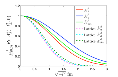
The superscript (1)1(1) on the TMDs indicates the first moment. In Fig.1, we have compared our model with the corresponding lattice resultsHagler . It is interesting to note that the above three lattice moments are almost identical when normalized to one at l2=0superscriptsubscript𝑙perpendicular-to20l_{\perp}^{2}=0. The diquark model also show similar behavior.

(1a)Refer to caption  (1b)Refer to caption
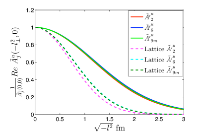

Figure 1: Comparison of Ai(l2,0)subscript𝐴𝑖subscriptsuperscriptl2perpendicular-to0{A}_{i}(-\textbf{l}^{2}_{\perp},0) in lattice QCD and AdS/QCD (a) for u and (b) for d quark. The doted lines are the Gaussian fits of the lattice data taken from Hagler , solid lines are the AdS/QCD results. In the plots, A~iq=ReA~iq(l2,0)Aiq(0,0)superscriptsubscript~𝐴𝑖𝑞𝑅𝑒superscriptsubscript~𝐴𝑖𝑞superscriptsubscript𝑙perpendicular-to20superscriptsubscript𝐴𝑖𝑞00\tilde{A}_{i}^{\prime q}=\frac{Re\tilde{A}_{i}^{q}(-l_{\perp}^{2},0)}{A_{i}^{q}(0,0)}.

IV quark densities

The Mellin moments of the TMDs can be interpreted as the densities of quarks inside the nucleon as:

ρUU(p)subscript𝜌𝑈𝑈subscriptpperpendicular-to\displaystyle\rho_{UU}(\textbf{p}_{\perp}) =\displaystyle= f1(1)(p2),subscriptsuperscript𝑓11subscriptsuperscriptp2perpendicular-to\displaystyle f^{(1)}_{1}(\textbf{p}^{2}_{\perp}), (43)
ρTL(p;S,λ)subscript𝜌𝑇𝐿subscriptpperpendicular-tosubscriptSperpendicular-to𝜆\displaystyle\rho_{TL}(\textbf{p}_{\perp};\textbf{S}_{\perp},\lambda) =\displaystyle= 12f1(1)(p2)+λ2p.SMg1T(1)(p2).12subscriptsuperscript𝑓11subscriptsuperscriptp2perpendicular-to𝜆2formulae-sequencesubscriptpperpendicular-tosubscriptSperpendicular-to𝑀subscriptsuperscript𝑔11𝑇subscriptsuperscriptp2perpendicular-to\displaystyle\frac{1}{2}f^{(1)}_{1}(\textbf{p}^{2}_{\perp})+\frac{\lambda}{2}\frac{\textbf{p}_{\perp}.\textbf{S}_{\perp}}{M}g^{(1)}_{1T}(\textbf{p}^{2}_{\perp}).

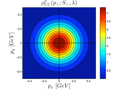
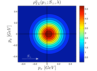
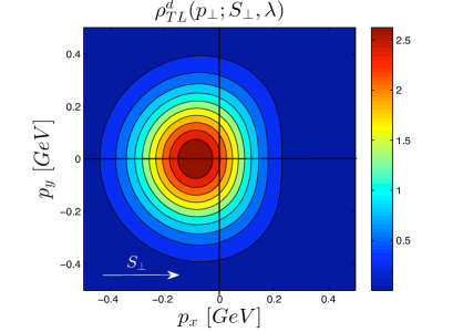
The density ρUU(p)subscript𝜌𝑈𝑈subscriptpperpendicular-to\rho_{UU}(\textbf{p}_{\perp}) is found when both nucleon and quark are unpolarised and the ρTL(p)subscript𝜌𝑇𝐿subscriptpperpendicular-to\rho_{TL}(\textbf{p}_{\perp}) is for transversely polarised nucleon. Considering the spin pointing along z𝑧z-direction and nucleon polarised in transverse x-direction,S=(1,0)subscriptSperpendicular-to10\textbf{S}_{\perp}=(1,0), the psubscriptpperpendicular-to\textbf{p}_{\perp}-densities of quarks in the two dimensional transverse momentum plane are plotted in Fig.(2).

In our model the unpolarised distributions, the unpolarised nucleon having unpolarised quarks inside, are symmetric for both u and d quarks as predicted from lattice data in Hagler . The values of p2ρUU=0.0569GeV2subscriptdelimited-⟨⟩subscriptsuperscriptp2perpendicular-tosubscript𝜌𝑈𝑈0.0569𝐺𝑒superscript𝑉2\langle\textbf{p}^{2}_{\perp}\rangle_{\rho_{UU}}=0.0569~{}GeV^{2} for u and p2ρUU=0.0725GeV2subscriptdelimited-⟨⟩subscriptsuperscriptp2perpendicular-tosubscript𝜌𝑈𝑈0.0725𝐺𝑒superscript𝑉2\langle\textbf{p}^{2}_{\perp}\rangle_{\rho_{UU}}=0.0725~{}GeV^{2} for d quarks.

The quark densities for unpolarized and polarized proton are shown in Fig2. Fig.2(a)-(b) represent the densities for u𝑢u and d𝑑d quark in unpolarized proton and Fig.2.(c)-(d), represent the same densities when proton is transversely polarised along x-axis, S=(1,0)subscript𝑆perpendicular-to10S_{\perp}=(1,0) and the quark spin pointing towards us with helicity λ=1𝜆1\lambda=1. The transverse momentum dependent densities of quarks are no longer axially symmetric in the transverse momentum plane. The peaks sift along the Ssubscript𝑆perpendicular-toS_{\perp} but in opposite direction with amplitudes pxρTL+66MeVsubscriptdelimited-⟨⟩subscriptp𝑥subscript𝜌𝑇𝐿66𝑀𝑒𝑉\langle\textbf{p}_{x}\rangle_{\rho_{TL}}\approx+66~{}MeV for u and pxρTL85MeVsubscriptdelimited-⟨⟩subscriptp𝑥subscript𝜌𝑇𝐿85𝑀𝑒𝑉\langle\textbf{p}_{x}\rangle_{\rho_{TL}}\approx-85~{}MeV for d quark. This sifting is because of non-zero g1T(1)(x,p2)subscriptsuperscript𝑔11𝑇𝑥subscriptsuperscriptp2perpendicular-tog^{(1)}_{1T}(x,\textbf{p}^{2}_{\perp}). The deformation in ρTLsubscript𝜌𝑇𝐿\rho_{TL} indicates that the transversely polarised nucleon is non-spherical, the u and d quarks have opposite directional distributions.

(a)Refer to caption  b)Refer to caption (c)Refer to caption  (d)Refer to caption
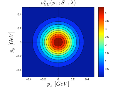
Figure 2: psubscriptpperpendicular-to\textbf{p}_{\perp}-densities of quarks in the two dimensional transverse momentum plane with λ=1𝜆1\lambda=1 and S=(1,0)subscriptSperpendicular-to10\textbf{S}_{\perp}=(1,0) for unpolarised and Transversely polarised proton corresponding to u and d quarksHagler . The figure-(c) is for u-d quarks having transversely polarised proton.

V Generalized parton distributions

Using the overlap formalism of light front wave functions, we evaluate the GPDs in light front quark-diquark model. The GPDs H𝐻H and E𝐸E are defined through the matrix element of the bilocal vector current on the light-front:

dy8πeixP+y/2P,λ|ψ(0)¯γ+ψ(y)|P,λ=𝑑superscript𝑦8𝜋superscript𝑒𝑖𝑥superscript𝑃superscript𝑦2quantum-operator-productsuperscript𝑃superscript𝜆¯𝜓0superscript𝛾𝜓𝑦𝑃𝜆absent\displaystyle\int\frac{dy^{-}}{8\pi}e^{ixP^{+}y^{-}/2}\langle P^{\prime},\lambda^{\prime}|~{}\bar{\psi(0)}\gamma^{+}\psi(y)~{}|P,\lambda\rangle=
12P+U¯λ(P)[H(x,ζ,t)γ++E(x,ζ,t)i2Mσ+αqα]Uλ(P),12superscript𝑃subscript¯𝑈superscript𝜆superscript𝑃delimited-[]𝐻𝑥𝜁𝑡superscript𝛾𝐸𝑥𝜁𝑡𝑖2𝑀superscript𝜎𝛼subscript𝑞𝛼subscript𝑈𝜆𝑃\displaystyle\!\!\!\!\!\!\frac{1}{2P^{+}}\bar{U}_{\lambda^{\prime}}(P^{\prime})\bigg{[}H(x,\zeta,t)\gamma^{+}+E(x,\zeta,t)\frac{i}{2M}\sigma^{+\alpha}q_{\alpha}\bigg{]}U_{\lambda}(P),
(45)

where P¯(P)¯𝑃superscript𝑃\bar{P}(P^{\prime}) is the initial(final) proton momentum, t=q2=(PP)2𝑡superscript𝑞2superscriptsuperscript𝑃𝑃2t=q^{2}=(P^{\prime}-P)^{2} and λ(λ)=±12𝜆superscript𝜆plus-or-minus12\lambda(\lambda^{\prime})=\pm\frac{1}{2} is the initial (final) proton spin. In terms of LFWF, the GPDs(for ζ=0𝜁0\zeta=0) are then obtained as

Hq(x,t)superscript𝐻𝑞𝑥𝑡\displaystyle H^{q}(x,t) =\displaystyle= d2𝐤16π3[ψ+q+(x,𝐤)ψ+q+(x,𝐤)\displaystyle\int\frac{d^{2}{\bf k}_{\perp}}{16\pi^{3}}~{}\bigg{[}\psi_{+q}^{+*}(x,{\bf k}_{\perp}^{\prime})\psi_{+q}^{+}(x,{\bf k}_{\perp}) (46)
+\displaystyle+ ψq+(x,𝐤)ψq+(x,𝐤)],\displaystyle\psi_{-q}^{+*}(x,{\bf k}_{\perp}^{\prime})\psi_{-q}^{+}(x,{\bf k}_{\perp})\bigg{]},
Eq(x,t)superscript𝐸𝑞𝑥𝑡\displaystyle E^{q}(x,t) =\displaystyle= 2Mq1iq2d2𝐤16π3[ψ+q+(x,𝐤)ψ+q(x,𝐤)\displaystyle-\frac{2M}{q^{1}-iq^{2}}\int\frac{d^{2}{\bf k}_{\perp}}{16\pi^{3}}~{}\bigg{[}\psi_{+q}^{+*}(x,{\bf k}_{\perp}^{\prime})\psi_{+q}^{-}(x,{\bf k}_{\perp}) (47)
+\displaystyle+ ψq+(x,𝐤)ψq(x,𝐤)],\displaystyle\psi_{-q}^{+*}(x,{\bf k}_{\perp}^{\prime})\psi_{-q}^{-}(x,{\bf k}_{\perp})\bigg{]},

where 𝐤=𝐤+(1x)𝐪superscriptsubscript𝐤perpendicular-tosubscript𝐤perpendicular-to1𝑥subscript𝐪perpendicular-to{\bf k}_{\perp}^{\prime}={\bf k}_{\perp}+(1-x){\bf q}_{\perp}. Integrating over ksubscript𝑘perpendicular-tok_{\perp}, we get

Hvq(x,t)subscriptsuperscript𝐻𝑞𝑣𝑥𝑡\displaystyle H^{q}_{v}(x,t) =\displaystyle\!\!= [F1(x)(1x)2+F2(x)(1x)4κ2M2log(1/x)\displaystyle\!\!\!\Big{[}F_{1}(x)(1-x)^{2}+F_{2}(x)(1-x)^{4}\frac{\kappa^{2}}{M^{2}\log(1/x)}
×\displaystyle\times (1Q24κ2log(1/x))]exp[Q24κ2log(1/x)],\displaystyle\!\!\!\!\!\!\!\!\!\!\Big{(}1-\frac{Q^{2}}{4\kappa^{2}}\log(1/x)\Big{)}\Big{]}\exp\bigg{[}-\frac{Q^{2}}{4\kappa^{2}}\log(1/x)\bigg{]}, (48)
Evq(x,t)subscriptsuperscript𝐸𝑞𝑣𝑥𝑡\displaystyle E^{q}_{v}(x,t) =\displaystyle= 2F3(x)(1x)3exp[Q24κ2log(1/x)].2subscript𝐹3𝑥superscript1𝑥3superscript𝑄24superscript𝜅21𝑥\displaystyle 2F_{3}(x)(1-x)^{3}\exp\bigg{[}-\frac{Q^{2}}{4\kappa^{2}}\log(1/x)\bigg{]}. (49)

The GPDs satisfy the physical conditions

01dxHq(x,0,)\displaystyle\int_{0}^{1}dxH^{q}(x,0,) =\displaystyle= nq,subscript𝑛𝑞\displaystyle n_{q},
01dxEq(x,0,)\displaystyle\int_{0}^{1}dxE^{q}(x,0,) =\displaystyle= κq,subscript𝜅𝑞\displaystyle\kappa_{q}, (50)

where nqsubscript𝑛𝑞n_{q} denotes the number of u𝑢u or d𝑑d valence quarks in the proton and κqsubscript𝜅𝑞\kappa_{q} is the anomalous magnetic moment of quark q𝑞q. Note that the exponential factors in both TMDs and GPDs come from the AdS/QCD wavefunction, but due to additional integration over the transverse momentum, the t𝑡t dependence in GPD is totally different from the p2superscriptsubscript𝑝perpendicular-to2p_{\perp}^{2} dependence in the TMDs. since Q2=q2=q2=tsuperscript𝑄2superscript𝑞2superscriptsubscript𝑞perpendicular-to2𝑡Q^{2}=-q^{2}=q_{\perp}^{2}=-t, the exponential factors in Eq.(48) and Eq.(49), can be written as exp[Q24κ2log(1/x)]=xαtsuperscript𝑄24superscript𝜅21𝑥superscript𝑥superscript𝛼𝑡\exp\big{[}-\frac{Q^{2}}{4\kappa^{2}}\log(1/x)\big{]}=x^{-\alpha^{\prime}t} where α=1/(4κ2)superscript𝛼14superscript𝜅2\alpha^{\prime}=1/(4\kappa^{2}), i.e., the GPDs show Regge behavior. But due to the extra (1x)2superscript1𝑥2(1-x)^{-2} factor in the exponentials, it is not possible to express TMDs in the Regge type form similar to GPDs.

V.1 Relations between TMDs and GPDs
Refer to caption
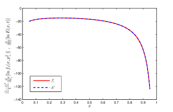
Figure 3: The variation of f1=(1x)24p2[lnf1(x,p2)]subscriptsuperscript𝑓1superscript1𝑥24subscriptsuperscript𝑝2perpendicular-todelimited-[]subscript𝑓1𝑥subscriptsuperscript𝑝2perpendicular-tof^{\prime}_{1}=\frac{(1-x)^{2}}{4}\frac{\partial}{\partial p^{2}_{\perp}}[\ln f_{1}(x,p^{2}_{\perp})] and E=|t|[lnE(x,t)]superscript𝐸𝑡delimited-[]𝐸𝑥𝑡E^{\prime}=\frac{\partial}{\partial|t|}[\ln E(x,t)].

The GPDs and TMDs satisfy a universal relation:

|t|[ln(GPD)]=(1x)24p2[ln(TMD)].𝑡delimited-[]GPDsuperscript1𝑥24subscriptsuperscript𝑝2perpendicular-todelimited-[]TMD\displaystyle\frac{\partial}{\partial|t|}[\ln({\rm GPD})]=\frac{(1-x)^{2}}{4}\frac{\partial}{\partial p^{2}_{\perp}}[\ln({\rm TMD})]. (51)

This result relies on the particular t𝑡t and p2superscriptsubscript𝑝perpendicular-to2p_{\perp}^{2} dependence of the GPDs and TMDs which comes from the AdS/QCD wave function. The relation is not exact for all the TMDs and GPDs, but numerically the differences are found to be insignificant.

Let us discuss the specific origin of this relation in some detail. The TMDs and GPDs have the two distinct exponential behavior which comes from the exponential behavior of the wavefunction predicted by AdS/QCD, but due to the extra integration over the transverse momentum transfer, the exponential in GPDs is completely different from that of TMDs. In case of GPDs, the t𝑡t (or Q2superscript𝑄2Q^{2}) behavior is of Regge type (xα+αtproportional-toabsentsuperscript𝑥𝛼superscript𝛼𝑡\propto x^{\alpha+\alpha^{\prime}t}) but it is rather Gaussian for TMDs.

We expect that this relation, being approximate and model-dependent, may reflect the physics of AdS/QCD duality (which is itself based on approximate conformal invariance and cannot be exact) and hold in more general context.

The relation has been demonstrated for the GPD E(x,t)𝐸𝑥𝑡E(x,t) and TMD f1(x,p2)subscript𝑓1𝑥superscriptsubscript𝑝perpendicular-to2f_{1}(x,p_{\perp}^{2}) in Fig.3.

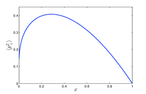
The GPDs obtained from the model satisfy the Regge behavior with the Regge slope α=1/(4κ2)superscript𝛼14superscript𝜅2\alpha^{\prime}=1/(4\kappa^{2}). The average value of Gaussian transverse momentum distribution is then obtained as

p2=(1x)24αln1/x=κ2(1x)2ln1/x,delimited-⟨⟩superscriptsubscript𝑝perpendicular-to2superscript1𝑥24superscript𝛼1𝑥superscript𝜅2superscript1𝑥21𝑥\displaystyle\langle p_{\perp}^{2}\rangle=\frac{(1-x)^{2}}{4\alpha^{\prime}\ln{1/x}}=\frac{\kappa^{2}(1-x)^{2}}{\ln{1/x}}, (52)

which takes the maximum value of p2max(255MeV)2subscriptdelimited-⟨⟩superscriptsubscript𝑝perpendicular-to2𝑚𝑎𝑥superscript255MeV2\langle p_{\perp}^{2}\rangle_{max}\approx(255\rm{MeV})^{2} for x1/3similar-to𝑥13x\sim 1/3.

Refer to caption
Figure 4: The xlimit-from𝑥x-dependence of average transverse momentum squared in the units of κ2superscript𝜅2\kappa^{2}

It is interesting that this value of x𝑥x naturally corresponding to average momentum of valence quark appears here as a maximum of elementary function (1x)2/ln(1/x)superscript1𝑥21𝑥(1-x)^{2}/\ln{(1/x)} implied by AdS/QCD. This expression also relies on the particular model and possibility to drop the above mentioned numerically small terms. Indeed, such completely different origin of the number naturally explained in the valence quarks picture may seem strange and may be accidental, although one cannot exclude that it is yet another manifestation of approximate AdS/QCD duality.

The magnitude of the transverse momentum is independent of quark flavor. Note that AdS/QCD warp parameter κ𝜅\kappa thus corresponds to the seemingly different quantities like Regge slope and average quark transverse momentum. Note also that the Regge slope relation to average transverse momentum was first found by V.N. Gribov in the framework of scalar ladders summation for soft Pomeron (having some similarity to the case under consideration because of limited transverse momentum) forming a “Heterotic Pomeron" Levin:1992ys while combining with hard BFKL Pomeron 111O.T. is indebted to L.N. Lipatov for pointing out that connection.
Refer to caption
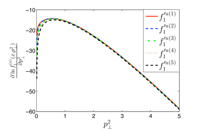
Figure 5: Illustration of Eq.(53).

The moments of f1(x,p)subscript𝑓1𝑥subscript𝑝perpendicular-tof_{1}(x,p_{\perp}) satisfy another interesting relation

P2[lnf1(1q)(p2)]subscriptsuperscript𝑃2perpendicular-todelimited-[]subscriptsuperscript𝑓1𝑞1subscriptsuperscript𝑝2perpendicular-to\displaystyle\frac{\partial}{\partial P^{2}_{\perp}}[\ln f^{(1q)}_{1}(p^{2}_{\perp})] similar-to-or-equals\displaystyle\simeq P2[lnf1(2q)(p2)]similar-to-or-equalssubscriptsuperscript𝑃2perpendicular-todelimited-[]subscriptsuperscript𝑓2𝑞1subscriptsuperscript𝑝2perpendicular-toabsent\displaystyle\frac{\partial}{\partial P^{2}_{\perp}}[\ln f^{(2q)}_{1}(p^{2}_{\perp})]\simeq
P2[lnf1(3q)(p2)]subscriptsuperscript𝑃2perpendicular-todelimited-[]subscriptsuperscript𝑓3𝑞1subscriptsuperscript𝑝2perpendicular-to\displaystyle\frac{\partial}{\partial P^{2}_{\perp}}[\ln f^{(3q)}_{1}(p^{2}_{\perp})] similar-to-or-equals\displaystyle\simeq P2[lnf1(nq)(p2)]similar-to-or-equalssubscriptsuperscript𝑃2perpendicular-todelimited-[]subscriptsuperscript𝑓𝑛𝑞1subscriptsuperscript𝑝2perpendicular-to\displaystyle\cdots\simeq\frac{\partial}{\partial P^{2}_{\perp}}[\ln f^{(nq)}_{1}(p^{2}_{\perp})] (53)

which is illustrated in Fig.5 for u𝑢u-quarks upto 555-th moments. We obtain similar plot for d𝑑d-quark also.

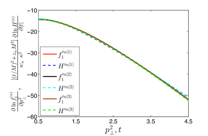
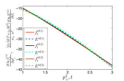
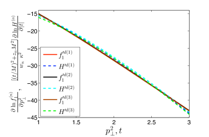
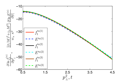
In the high momentum region the slopes of the n𝑛nth moments of TMDs and GPDs satisfy the following empirical but a relation general to all n𝑛n (numerically checked upto n=5𝑛5n=5):

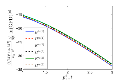
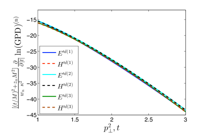
|t|ln(GPD)(n)(t)wnqκ2[(tM)2+znqM2]P2lnf1(n)(p2),\displaystyle\!\!\!\!\!\!\frac{\partial}{\partial|t|}\ln({\rm GPD})^{(n)}(t)\simeq\frac{w^{q}_{n}\kappa^{2}}{[(\frac{t}{M})^{2}+z^{q}_{n}M^{2}]}\frac{\partial}{\partial P^{2}_{\perp}}\ln f^{(n)}_{1}(p^{2}_{\perp}), (54)

where the superscript (n)𝑛(n) stands for the n𝑛n-th moment. znqsubscriptsuperscript𝑧𝑞𝑛z^{q}_{n} and wnqsubscriptsuperscript𝑤𝑞𝑛w^{q}_{n} are given by znu=2+0.5(n1),wnu=1.50.12(n1)formulae-sequencesubscriptsuperscript𝑧𝑢𝑛20.5𝑛1subscriptsuperscript𝑤𝑢𝑛1.50.12𝑛1z^{u}_{n}=2+0.5(n-1),~{}w^{u}_{n}=1.5-0.12(n-1) when the GPD is Hu(x,t)subscript𝐻𝑢𝑥𝑡H_{u}(x,t) and znu=1.7+(n1)0.55,wnu=1.5(n1)0.12formulae-sequencesubscriptsuperscript𝑧𝑢𝑛1.7𝑛10.55subscriptsuperscript𝑤𝑢𝑛1.5𝑛10.12z^{u}_{n}=1.7+(n-1)0.55,~{}w^{u}_{n}=1.5-(n-1)0.12 for Eu(x,t)subscript𝐸𝑢𝑥𝑡E_{u}(x,t) and for the d-quark the values are znd=1.06+(n1)0.385,wnd=1.15(n1)0.105formulae-sequencesubscriptsuperscript𝑧𝑑𝑛1.06𝑛10.385subscriptsuperscript𝑤𝑑𝑛1.15𝑛10.105z^{d}_{n}=1.06+(n-1)0.385,~{}w^{d}_{n}=1.15-(n-1)0.105 for Hdsubscript𝐻𝑑H_{d} and znd=1.7+(n1)0.55,wnd=1.12(n1)0.1formulae-sequencesubscriptsuperscript𝑧𝑑𝑛1.7𝑛10.55subscriptsuperscript𝑤𝑑𝑛1.12𝑛10.1z^{d}_{n}=1.7+(n-1)0.55,~{}w^{d}_{n}=1.12-(n-1)0.1 for Edsubscript𝐸𝑑E_{d}. These relations for u𝑢u and d𝑑d quarks are illustrated in Figs.6 for first three moments.

(a)Refer to caption  (b)Refer to caption
(c)Refer to caption  (b)Refer to caption

Figure 6: Plot of Eq.(54) forf1(x,p)subscript𝑓1𝑥subscript𝑝perpendicular-tof_{1}(x,p_{\perp}) and (a) Eu(x,t)subscript𝐸𝑢𝑥𝑡E_{u}(x,t), (b) Hu(x,t)subscript𝐻𝑢𝑥𝑡H_{u}(x,t), (c)Ed(x,t)subscript𝐸𝑑𝑥𝑡E_{d}(x,t) and (d) Hd(x,t)subscript𝐻𝑑𝑥𝑡H_{d}(x,t) for n=1,2,3𝑛123n=1,2,3.

(a) Refer to caption  (b)Refer to caption

Figure 7: The Eq.(55)is plotted with n=1,2,3𝑛123n=1,2,3 for (a) u quark and (b) d quark.

This difference of transverse momentum dependence may be qualitatively explained by the different x-dependence of exponential factors in the corresponding integrand. As for GPDs it is just exp(|tαlnx|)𝑡superscript𝛼𝑥\exp(-|t\alpha^{\prime}\ln{x}|), for larger t𝑡t the larger values of x𝑥x contribute so that the decrease of the moments is only power-like, the notable example represented by electromagnetic form factors. At the same time, for TMDs the similar factor is exp(|p2αlnx/4(1x)2|)superscriptsubscript𝑝perpendicular-to2superscript𝛼𝑥4superscript1𝑥2\exp(-|p_{\perp}^{2}\alpha^{\prime}\ln{x}/4(1-x)^{2}|) so that it is suppressing the contributions of both large and small x𝑥x and only the region of x1/3similar-to𝑥13x\sim 1/3 corresponding to the maximum at Fig.4 contributes. As a result, while using the saddle-point method, the corresponding exponential factor may be taken out of the integral and the main dependence of TMD moments on p2superscriptsubscript𝑝perpendicular-to2p_{\perp}^{2} is an exponential one! This explains the extra factor in Eq.(54). This also may be the the reason of approximate “factorization" of x𝑥x and psubscript𝑝perpendicular-top_{\perp} dependence of TMDs which is not contradicting to lattice QCD data Hagler ; lattice . Such factorization ansatz is also used in the phenomenological parameterizations and experimental extractions of the TMDsanselmino .

(a)Refer to caption  (b)Refer to caption
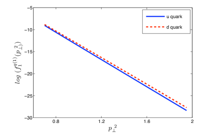
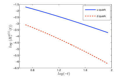
Figure 8: (a) The p2superscriptsubscript𝑝perpendicular-to2p_{\perp}^{2} dependence of the first moments of the TMD f1q(x,p2)superscriptsubscript𝑓1𝑞𝑥superscriptsubscript𝑝perpendicular-to2f_{1}^{q}(x,p_{\perp}^{2}) and (b) t𝑡t-dependence of the first moment of the GPD Hvq(x,t)superscriptsubscript𝐻𝑣𝑞𝑥𝑡H_{v}^{q}(x,t)

It is interesting to note that with the same values of znsubscript𝑧𝑛z_{n} and wnsubscript𝑤𝑛w_{n} one can relate the slopes of the two GPDs also

[(tM)2+znq,EM2]wnq,Eκ2|t|[lnE(n)(t)]similar-to-or-equalsdelimited-[]superscript𝑡𝑀2subscriptsuperscript𝑧𝑞𝐸𝑛superscript𝑀2subscriptsuperscript𝑤𝑞𝐸𝑛superscript𝜅2𝑡delimited-[]superscriptEntabsent\displaystyle\frac{[(\frac{t}{M})^{2}+z^{q,E}_{n}M^{2}]}{w^{q,E}_{n}\kappa^{2}}\frac{\partial}{\partial|t|}[\ln\rm{E}^{(n)}(t)]\simeq
[(tM)2+znq,HM2]wnq,Hκ2|t|[lnH(n)(t)],delimited-[]superscript𝑡𝑀2subscriptsuperscript𝑧𝑞𝐻𝑛superscript𝑀2subscriptsuperscript𝑤𝑞𝐻𝑛superscript𝜅2𝑡delimited-[]superscriptHnt\displaystyle~{}~{}~{}\frac{[(\frac{t}{M})^{2}+z^{q,H}_{n}M^{2}]}{w^{q,H}_{n}\kappa^{2}}\frac{\partial}{\partial|t|}[\ln\rm{H}^{(n)}(t)], (55)

as can be seen in Fig.7. Since, the moments of different distributions are calculate in lattice QCD, these relations can help to check the consistency of model calculations with lattice results.

To provide some quantitative ground for this picture we calculated the transverse momentum dependence of the moments of TMDs and GPDs. In Fig.8 (a), we have shown the first moment of f1q(x,p2)superscriptsubscript𝑓1𝑞𝑥superscriptsubscript𝑝perpendicular-to2f_{1}^{q}(x,p_{\perp}^{2}). It clearly indicates that the first moment of the TMD has exponential dependence on the transverse momentum p2superscriptsubscript𝑝perpendicular-to2p_{\perp}^{2}. This behavior of the moments is a necessary condition of the mentioned factorization of x𝑥x and psubscript𝑝perpendicular-top_{\perp} dependencies, At the same time, Fig.8(b), indicates that for large t𝑡-t, the GPD follows a power law behavior with t𝑡-t which is naturally related to the Regge Parameterization.

VI Discussion

We calculated the TMDs in the framework of soft wall AdS/QCD based diquark model of the nucleon and performed the systematic exploration of their properties and comparison with GPDs. We tested the number of relations and inequalities for TMDs.

The fit of data leads to the value of warp parameter κ400MeV𝜅400𝑀𝑒𝑉\kappa\approx 400MeV.

The new relation between t𝑡t-dependence of GPDs and psubscript𝑝perpendicular-top_{\perp}-dependence of TMDs is found. It is approximate and model dependent, but may express the physics of approximate AdS/QCD duality, which requires further checks. The x dependence of average transverse momentum squared or TMDs is calculated. While the GPDs exhibit the Regge behavior combining the exponential dependence on t𝑡t at fixed x𝑥x with the power dependence of the moments, related to the formfactors, the TMDs exhibit the gaussian dependence on psubscript𝑝perpendicular-top_{\perp} both at fixed x𝑥x and after integration over x𝑥x. This may be the reason for approximate factorization of x𝑥x and psubscript𝑝perpendicular-top_{\perp} dependencies of TMDs compatible with lattice QCD and used in phenomenological analysis.

We thank A. V. Efremov, L.N. Lipatov and C. Lorcé for useful discussions and comments. D.C. is grateful to BLTP, JINR, where this work was completed, for warm hospitality. O.T. was supported in part by RFBR grant 14-01-00647.

References

  • (1) A. Chekanov et. al, ZEUS collaboration, Phys. Lett. B 573, 46(2003), N. D’Hose et. al, Eur. Phys. J. A 19,47 (2004); M. Aleksev et. al, COMPASS Collaboration, Phys. Lett. B 673, 127 (2009); A. Airapetian et. al, HERMES collaboration, Phys. Rev. Lett 103, 152002 (2009); H. Avakian et. al, CLAS collaboration, Phys. Rev. Lett. 105, 162002 (2010).
  • (2) S. J. Brodsky and G. F. de Teramond, Phys. Rev. Lett. 96, 201601 (2006).
  • (3) J. Collins, Int. J. Mod. Phys. Conf. Ser.  4, 85 (2011).
  • (4) M. Diehl, Phys. Rept. 388, 41 (2003).
  • (5) R. Jakob, P. J. Mulders and J. Rodrigues, Nucl. Phys. A 626, 937 (1997).
  • (6) A. Bacchetta, F. Conti and M. Radici, Phys. Rev. D 78, 074010 (2008).
  • (7) H. Avakian, A. V. Efremov, P. Schweitzer and F. Yuan, Phys. Rev. D 81, 074035 (2010).
  • (8) A. V. Efremov, P. Schweitzer, O. V. Teryaev and P. Zavada, Phys. Rev. D 80, 014021 (2009).
  • (9) A. V. Efremov, P. Schweitzer, O. V. Teryaev and P. Zavada, Phys. Rev. D 83, 054025 (2011).
  • (10) S. Meissner, A. Metz and K. Goeke, Phys. Rev. D 76, 034002 (2007).
  • (11) D. Mueller and D. S. Hwang, PoS QNP 2012, 059 (2012).
  • (12) O. Teryaev, EPJ Web Conf.  85, 02008 (2015).
  • (13) T. Gutsche, V.E. Lyubovitskij, I. Schmidt, A. Vega, Phys. Rev. D 89, 054033 (2014).
  • (14) C. Mondal and D. Chakrabarti, Eur. Phys. J. C 75, no. 6, 261 (2015).
  • (15) D. Chakrabarti, C. Mondal, Phys. Rev. D 88, 073006 (2013).
  • (16) D. Chakrabarti and C. Mondal, Phys. Rev. D 92, 074012 (2015).
  • (17) S. J. Brodsky and G. F. de Téramond, arXiv:1203.4025, Phys. Rev. D. 84, 075012 (2011).
  • (18) G. Karl and J. E. Paton, Phys. Rev. D 30, 238 (1984).
  • (19) Ph. Hagler, B.U.Musch, J.W.Negele, A.Schafer, Eur. phys.Lett. 88, 61001(2009);  B.U.Musch, arXiv: 0907.2381 [hep-lat] 2009.
  • (20) J. Soffer, Phys. Rev. Lett 74, 1292 (1995).
  • (21) A. Bacchetta, M. Boglione, A. Henneman, P. J. Mulders, Phys. Rev. Lett. 85, 712 (2000).
  • (22) C. Lorcé and B. Pasquini, Phys. Rev. D 84, 034039 (2011).
  • (23) E. Levin and C. I. Tan, In *Santiago de Compostela 1992, Proceedings, Multiparticle dynamics* 568-575 and Fermilab Batavia - FERMILAB-Conf-92-391 (92/09,rec.Jan.93) 9 p. (303600) Brown Univ. Providence - BROWN-HET-889 (92/09,rec.Jan.93) 9 p. [hep-ph/9302308].
  • (24) B. Musch, P. Hägler, J. Negele and A. Schäfer, Phys. Rev. D. 83, 094507 (2011).
  • (25) M. Anselmino et. al., Phys. Rev. D 75, 054032 (2007); C. Lefky and A. Prokudin, Phys. Rev. D 91, 034010 (2015); M. Anselmino, TMD phenomenology, talk presented at Light Cone 2015, and the references therein:
      https://agenda.infn.it/getFile.py/access?contribId
    =16&sessionId=7&resId=0&materialId=slides&confId=9011