Learning Deep Generative Models with Doubly Stochastic MCMC

Abstract

We present doubly stochastic gradient MCMC, a simple and generic method for (approximate) Bayesian inference of deep generative models (DGMs) in a collapsed continuous parameter space. At each MCMC sampling step, the algorithm randomly draws a mini-batch of data samples to estimate the gradient of log-posterior and further estimates the intractable expectation over hidden variables via a neural adaptive importance sampler, where the proposal distribution is parameterized by a deep neural network and learnt jointly. We demonstrate the effectiveness on learning various DGMs in a wide range of tasks, including density estimation, data generation and missing data imputation. Our method outperforms many state-of-the-art competitors.

1 Introduction

Learning deep models that consist of multi-layered representations has obtained state-of-the-art performance in many tasks (Bengio et al., 2014; Hinton et al., 2006), partly due to their ability on capturing high-level abstractions. As an important family of deep models, deep generative models (DGMs) (Hinton et al., 2006; Salakhutdinov & Hinton, 2009) can answer a wide range of queries by performing probabilistic inference, such as inferring the missing values of input data, which is beyond the scope of recognition networks such as deep neural networks.

However, probabilistic inference with DGMs is challenging, especially when a Bayesian formalism is adopted, which is desirable to protect the DGM from overfitting (MacKay, 1992; Neal, 1995) and to perform sparse Bayesian inference (Gan et al., 2015b) or nonparametric inference (Adams et al., 2010) to learn the network structure. For Bayesian methods in general, the posterior inference often involves intractable integrals because of several potential factors, such as that the space is extremely high-dimensional and that the Bayesian model is non-conjugate. To address the challenges, approximate methods have to be adopted, including variational (Jordan et al., 1999; Saul et al., 1996) and Markov chain Monte Carlo (MCMC) methods (Robert & Casella, 2005).

Much progress has been made on stochastic variational methods for DGMs (Kingma & Welling, 2014; Rezende et al., 2014; Ranganath et al., 2014), under some mean-field or parameterization assumptions. One key feature of such variational methods is that they marry ideas from deep neural networks to parameterize the variational distribution by a recognition network and jointly learn the parameters by optimizing a variational bound. In contrast, little work has been done on extending MCMC methods to learn DGMs in a Bayesian setting, which are often more accurate, except a few exceptions. Gan et al. (2015b) present a Gibbs sampler for deep sigmoid belief networks with a sparsity-inducing prior via data augmentation, Adams et al. (2010) present a Metropolis-Hastings method for cascading Indian buffet process and Li et al. (2016) develop a high-order stochastic gradient MCMC method and apply to deep Poisson factor analysis (Gan et al., 2015a).

In this paper, we present a simple and generic method, named doubly stochastic gradient MCMC, to improve the efficiency of performing Bayesian inference on DGMs. By drawing samples in the collapsed parameter space, our method extends the recent work on stochastic gradient MCMC (Welling & Teh, 2011; Ahn et al., 2012; Chen et al., 2014; Ding et al., 2014) to deal with the challenging task of posterior inference with DGMs. Besides the stochasticity of randomly drawing a mini-batch of samples in stochastic approximation, our algorithm introduces an extra dimension of stochasticity to estimate the intractable gradients by randomly drawing the hidden variables in DGMs. The sampling can be done via a Gibbs sampler, which however has a low mixing rate in high dimensional spaces. To address that, we develop a neural adaptive importance sampler (NAIS), where the adaptive proposal is parameterized by a recognition network and the parameters are optimized by descending inclusive KL-divergence. By combining the two types of stochasticity, we construct an asymptotically unbiased estimate of the gradient in the continuous parameter space. Then, a stochastic gradient MCMC method is applied with guarantee to (approximately) converge to the target posterior when the learning rates are set under some proper annealing scheme.

Our method can be widely applied to the DGMs with either discrete or continuous hidden variables. In experiments, we demonstrate the efficacy on learning various DGMs, such as deep sigmoid belief networks (Mnih & Gregor, 2014), for density estimation, data generation and missing value imputation. Our results show that we can outperform many strong competitors for learning DGMs.

2 Related Work

Recently, there has been a lot of interest in developing variational methods for DGMs. One common strategy for dealing with the intractable posterior distribution is to approximate it with a recognition (or inference) network, and a variational lower bound is then optimized (Kingma & Welling, 2014; Mnih & Gregor, 2014). Note in these methods the gradients are also estimated doubly stochastically. Kingma & Welling (2014) and Mnih & Gregor (2014) adopt variance reduction techniques to make these methods practically applicable. Titsias & Lázaro-Gredilla (2014) propose a so-called “doubly stochastic variational inference” method for non-conjugate Bayesian inference. We are inspired by these methods when naming ours.

The reweighted wake-sleep (RWS) (Bornschein & Bengio, 2015) and importance weighted autoencoder (IWAE) (Burda et al., 2015) directly estimate the log-likelihood (as well as its gradient) via importance sampling, where the proposal distribution is characterized by a recognition model. These methods reduce the gap between the variational bound and the log-likelihood, which is shown much tighter than that in Kingma & Welling (2014). Such tighter bound results in an asymptotically unbiased estimator of its gradient. We draw inspiration from these variational methods to build our MCMC samplers.

Our work is closely related to the recent progress on neural adaptive proposals for sequential Monte Carlo (NASMC) (Gu et al., 2015). Different from our work, NASMC deals with dynamical models such as Hidden Markov models and adopts recurrent neural network as the proposal. We use a similar KL-divergence as NASMC to learn the proposal.

Finally, Gan et al. (2015a) adopt a Monte Carlo estimate via Gibbs sampling to the intractable gradients under a stochastic MCMC method particularly for topic models. Besides a general perspective which is applicable to various types of DGM models, we propose a neural adaptive importance sampler which is more efficient than Gibbs sampling and leads to better estimates.

3 Doubly Stochastic Gradient MCMC for Deep Generative Models

We now present the doubly stochastic gradient MCMC for deep generative models.

3.1 Deep Generative Models

Let $\mathbf{X}=\{\mathbf{x}_{n}\}^{N}_{n=1}$ be a given dataset with $N$ i.i.d. samples. A deep generative model (DGM) assumes that each sample $\mathbf{x}_{n}\in\mathbb{R}^{D}$ is generated from a vector of hidden variables $\mathbf{z}_{n}\in\mathbb{R}^{H}$, which itself follows some prior distribution $p(\mathbf{z}|\bm{\alpha})$. Let $p(\mathbf{x}|\mathbf{z},\bm{\beta})$ be the likelihood model. The joint probability of a DGM is as follows:

$$p(\mathbf{X},\mathbf{Z}|\bm{\theta})=\prod^{N}_{n=1}p(\mathbf{z}_{n}|\bm{\alpha})p(\mathbf{x}_{n}|\mathbf{z}_{n},\bm{\beta}),$$ (1)

where $\bm{\theta}:=(\bm{\alpha},\bm{\beta})$. Depending on the structure of $\mathbf{z}$, various DGMs have been developed, such as deep belief networks (Hinton et al., 2006), deep sigmoid belief networks (Mnih & Gregor, 2014), and deep Boltzmann machines (Salakhutdinov & Hinton, 2009).

For most DGMs, the hidden variables $\mathbf{z}$ are often assumed to have a directed multi-layer representation $\mathbf{z}=\{\mathbf{z}^{(l)}\}_{l=1}^{L}$, where $L$ is the number of hidden layers. Then the prior distribution has the factorization form:

$$p(\mathbf{z}|\bm{\theta})=p(\mathbf{z}^{(L)}|\bm{\theta})\prod^{L-1}_{l=1}p(\mathbf{z}^{(l)}|\mathbf{z}^{(l+1)},\bm{\theta}),$$ (2)

where $p(\mathbf{z}^{(l)}|\mathbf{z}^{(l+1)},\bm{\theta})$ is defined by some conditional stochastic layer that takes $\mathbf{z}^{(l+1)}$ as input and generates samples $\mathbf{z}^{(l)}$. The likelihood model is further assumed to be a conditional stochastic layer again:

$$p(\mathbf{x}|\mathbf{z},\bm{\theta})=p(\mathbf{x}|\mathbf{z}^{(1)},\bm{\theta}),$$ (3)

where the samples are generated conditioned on the lowest hidden layer only.

Various conditional stochastic layers have been developed. In the following we briefly summarize the layers used in our experiments:

Sigmoid Belief Network layer (SBN): A SBN layer (Saul et al., 1996) is a directed graphical model that defines the conditional probability of each independent binary variable $z^{(l)}_{i}$ given the upper layer $\mathbf{z}^{(l+1)}$ as follows:

$$p(z^{(l)}_{i}=1|\mathbf{z}^{(l+1)})=\sigma(\mathbf{W}_{i,:}\mathbf{z}^{(l+1)}+b_{i}),$$ (4)

where $\sigma(x)\!=\!1/(1+e^{-x})$ is the sigmoid function, $\mathbf{W}_{i,:}$ denotes the $i$-th row of the weight matrix and $b_{i}$ is the bias.

Deep Autoregressive Network layer (DARN): A DARN (Gregor et al., 2014) layer assumes in-layer connections on the SBN layer. It defines the probability of each binary variable $z^{(l)}_{i}$ conditioned on both the upper layer $\mathbf{z}^{(l+1)}$ and the previous $\mathbf{z}^{(l)}_{<i}$ in the same layer:

$$p(z^{(l)}_{i}=1|\mathbf{z}^{(l)}_{<i},\mathbf{z}^{(l+1)})=\sigma(\mathbf{U}_{i,:}\mathbf{z}^{(l+1)}+\mathbf{W}_{i,<i}\mathbf{z}^{(l)}_{<i}+b_{i}),$$

where $\mathbf{z}^{(l)}_{<i}$ refers to $(z^{(l)}_{1},\cdots,z^{(l)}_{i-1})^{\top}$ and $\mathbf{W}_{i,<i}$ denotes the first $i$ elements of the $i$-th row of the in-layer connection weight matrix.

Conditional NADE layer: The NADE (Larochelle & Murray, 2011) models the distribution of high-dimensional discrete variables $\mathbf{x}$ autoregressively with an internal MLP (Bengio & Bengio, 2000). The dependency between the variables is captured by a single-hidden-layer feed-forward neural network:

$$p(x_{i}=1|\mathbf{x}_{<i})=\sigma(\mathbf{V}_{i,:}\sigma(\mathbf{W}_{:,<i}\mathbf{x}_{<i}+\mathbf{a})+b_{i}).$$

Boulanger-Lewandowski et al. (2012) and Bornschein & Bengio (2015) amend this model to a conditional NADE layer:

$$p(z^{(l)}_{i}=1| \mathbf{z}^{(l)}_{<i},\mathbf{z}^{(l+1)})=\sigma\Big{(}\mathbf{V}_{i,:}\sigma(\mathbf{W}_{:,<i}\mathbf{z}^{(l)}_{<i}+$$ (5)

$$\mathbf{U}\mathbf{z}^{(l+1)}+\mathbf{a})+\mathbf{R}_{i,:}\mathbf{z}^{(l+1)}+b_{i}\Big{)},$$

where we use $\mathbf{W}_{:,<i}$ to refer the sub-matrix consisting the first $i$ columns of $\mathbf{W}$.

Variational Auto-Encoder layer (VAE): VAE (Kingma & Welling, 2014) differs from the above layers in that its output can be binary or real-valued variables. It contains an internal MLP $f(\mathbf{z}^{(l+1)})$ which encodes the parameters of the distribution $p(\mathbf{z}^{(l)}|\mathbf{z}^{(l+1)})$. The MLP may itself contain multiple deterministic layers. For binary output variable, the distribution of each individual variable is:

$$p(z^{(l)}_{i}=1|\mathbf{z}^{(l+1)})=\sigma(\mathbf{W}_{i,:}f(\mathbf{z}^{(l+1)})+b_{i}).$$ (6)

For real-value output variable, the distribution of each independent variable $z^{(l)}_{i}$ is a normal distribution whose mean and variance are as follows:

$$\mu_{i}= \mathbf{W}_{{\scriptscriptstyle\bm{\mu}}i,:}f(\mathbf{z}^{(l+1)})+b_{{\scriptscriptstyle\bm{\mu}}i},$$ (7)

$$\log\sigma_{i}^{2}= \mathbf{W}_{{\scriptscriptstyle\bm{\sigma}}i,:}f(\mathbf{z}^{(l+1)})+b_{{\scriptscriptstyle\bm{\sigma}}i}.$$

Top layer and Likelihood model: The likelihood model in Eqn. (3) can be obtained by treating $\mathbf{x}$ as $\mathbf{z}^{(0)}$. The distribution of top layer $p(\mathbf{z}^{(L)}|\bm{\theta})$, which has no ancestral layer, can be obtained by simply treating the input as $\bm{0}$ vector or setting to fixed distribution, e.g., standard normal for the VAE layer (Kingma & Welling, 2014). Detailed description of the layers and the model construction can be found in Supplementary Material.

3.2 Variational MLE for DGMs

Learning DGMs is often very challenging due to the intractability of posterior inference. One popular type of methods resort to stochastic variational methods under the maximum likelihood estimation (MLE) framework, $\hat{\bm{\theta}}=\operatornamewithlimits{argmax}_{\bm{\theta}}\log p(\mathbf{X}|\bm{\theta})$. These methods commonly utilize some variational distribution $q(\mathbf{z}|\mathbf{x};\bm{\phi})$ to approximate the true posterior $p(\mathbf{z}|\mathbf{x},\bm{\theta})$. For DGMs, the variational distribution $q(\mathbf{z}|\mathbf{x};\bm{\phi})$ can be formalized as a recognition model (or inference network) (Kingma & Welling, 2014; Mnih & Gregor, 2014; Bornschein & Bengio, 2015), which takes $\mathbf{x}$ as inputs and outputs $\mathbf{z}$ stochastically. Specifically, for the DGMs with multi-layer representation $\mathbf{z}=\{\mathbf{z}^{(l)}\}_{l=1}^{L}$ described in Sec. 3.1, the variational distribution can be formulated as:

$$q(\mathbf{z}|\mathbf{x},\bm{\phi})=q(\mathbf{z}^{(1)}|\mathbf{x},\bm{\phi})\prod^{L-1}_{l=1}q(\mathbf{z}^{(l+1)}|\mathbf{z}^{(l)},\bm{\phi}),$$ (8)

where each $q(\mathbf{z}^{(l+1)}|\mathbf{z}^{(l)},\bm{\phi})$ and $q(\mathbf{z}^{(1)}|\mathbf{x},\bm{\phi})$ are again defined by some stochastic layers parametrized by $\bm{\phi}$. With the variational distribution, a variational bound of the log-likelihood $\log p(\mathbf{X}|\bm{\theta})$ can be derived and optimized, e.g., the variational lower bound in (Kingma & Welling, 2014) and a tighter bound in (Burda et al., 2015).

However, the variational bound is often intractable to compute analytically for DGMs. To address this challenge, recent progress (Kingma & Welling, 2014; Rezende et al., 2014; Mnih & Gregor, 2014) has adopted hybrid Monte Carlo and variational methods, which approximate the intractable expectations and their gradients over the parameters $(\bm{\theta},\bm{\phi})$ via some unbiased Monte Carlo estimates. Furthermore, to handle large-scale datasets, stochastic optimization (Robbins & Monro, 1951; Bottou, 1998) of the variational objective can be used with a suitable learning rate annealing scheme. Note variance reduction is a key part of these methods to have fast and stable convergence.

3.3 Doubly Stochastic Gradient MCMC

We consider the Bayesian setting to infer the posterior distribution $p(\bm{\theta},\mathbf{Z}|\mathbf{X})\propto p_{0}(\bm{\theta})p(\mathbf{Z}|\bm{\theta})p(\mathbf{X}|\mathbf{Z},\bm{\theta})$ or its marginal distribution $p(\bm{\theta}|\mathbf{X})$, by assuming some prior $p_{0}(\bm{\theta})$. A Bayesian formalism of deep learning enjoys several advantages, such as preventing the model from overfitting and performing sparse/nonparametric Bayesian inference, as mentioned before. However, except a handful of special examples, the posterior distribution is intractable to infer. Though variational methods can be developed as in (Kingma & Welling, 2014; Rezende et al., 2014; Mnih & Gregor, 2014; Bornschein & Bengio, 2015), under some mean-field or parameterization assumptions, they often require non-trivial model-specific deviations and may lead to inaccurate approximation when the assumptions are not properly made. Here, we consider MCMC methods, which are more generally applicable and can asymptotically approach the target posterior.

A straightforward application of MCMC methods can be Gibbs sampling or stochastic gradient MCMC (Welling & Teh, 2011; Ahn et al., 2012; Chen et al., 2014; Ding et al., 2014). However, a Gibbs sampler can suffer from the random-walk behavior in high-dimensional spaces. Furthermore, a Gibbs sampler would need to process all data at each iteration, which is prohibitive when dealing with large-scale datasets. The stochastic gradient MCMC methods can lead to significant speedup by exploring statistical redundancy in large datasets; but they require that the sample space is continuous, which is not true for many DGMs, such as deep sigmoid belief networks that have discrete hidden variables. Below, we present a doubly stochastic gradient MCMC with general applicability.

3.3.1 General Procedure

We make the mildest assumption that the parameter space is continuous and the log joint distribution $\log p(\mathbf{x},\mathbf{z}|\bm{\theta})$ is differentiable with respect to the model parameters $\bm{\theta}$ almost everywhere except a zero-mass set. Such an assumption is true for almost all existing DGMs. Then, our method draws samples in a collapsed space that involves the model parameters $\bm{\theta}$ only, by integrating out the hidden variables $\mathbf{z}$:

$$p(\bm{\theta}|\mathbf{X})=\frac{1}{p(\mathbf{X})}p_{0}(\bm{\theta})\prod_{n=1}^{N}\int p(\mathbf{x}_{n},\mathbf{z}_{n}|\bm{\theta})\leavevmode\nobreak\ \mathrm{d}\mathbf{z}_{n},$$ (9)

where for discrete variables the integral will be a summation. Then the gradient of the log-posterior is $\nabla_{\bm{\theta}}\log p(\bm{\theta}|\mathbf{X})=\nabla_{\bm{\theta}}\log p_{0}(\bm{\theta})+\sum_{n=1}^{N}\nabla_{\bm{\theta}}\log p(\mathbf{x}_{n}|\bm{\theta}),$ where the second term can be calculated as:

$$\nabla_{\bm{\theta}}\log p(\mathbf{x}|\bm{\theta}) =\frac{1}{p(\mathbf{x}|\bm{\theta})}\frac{\partial}{\partial\bm{\theta}}\int p(\mathbf{x},\mathbf{z}|\bm{\theta})\leavevmode\nobreak\ \mathrm{d}\mathbf{z}$$

$$=\int\frac{p(\mathbf{x},\mathbf{z}|\bm{\theta})}{p(\mathbf{x}|\bm{\theta})}\frac{\partial}{\partial\bm{\theta}}\log p(\mathbf{x},\mathbf{z}|\bm{\theta})\leavevmode\nobreak\ \mathrm{d}\mathbf{z}$$

$$=\mathbb{E}_{p(\mathbf{z}|\mathbf{x},\bm{\theta})}\left[\frac{\partial}{\partial\bm{\theta}}\log p(\mathbf{x},\mathbf{z}|\bm{\theta})\right].$$ (10)

With the above gradient, we can adopt a stochastic gradient MCMC (SG-MCMC) method to draw samples of $\bm{\theta}$. We consider the stochastic gradient Nosé-Hoover thermostat (SGNHT) (Ding et al., 2014). Note our method can be naturally extended to other SG-MCMC methods, e.g., stochastic gradient Langevin dynamics (Welling & Teh, 2011), stochastic gradient Hamiltonian Monte Carlo (Chen et al., 2014) and high-order stochastic gradient thermostats (Li et al., 2016). SGNHT defines a potential energy $U(\bm{\theta})=-\log p(\bm{\theta}|\mathbf{X})$ where $p(\bm{\theta}|\mathbf{X})$ is the target posterior distribution, and use a random mini-batch $B$ of the data $\mathbf{X}$ to approximate the true gradient of the potential energy:

$$\!\nabla_{\bm{\theta}}\tilde{U}(\bm{\theta})\!=\!-\nabla_{\bm{\theta}}\log p_{0}(\bm{\theta})\!-\!\frac{N}{|B|}\!\sum_{n\in B}\!\nabla_{\bm{\theta}}\log p(\mathbf{x}_{n}|\bm{\theta}).$$ (11)

We follow Gan et al. (2015a) to use the multivariate version of SGNHT that generate samples by simulating the dynamics as follows:

$$\bm{\theta}_{t+1} =\bm{\theta}_{t}+\lambda\mathbf{p}_{t},$$ (12)

$$\mathbf{p}_{t+1} =\mathbf{p}_{t}-\lambda\bm{\xi}_{t}\odot\mathbf{p}_{t}-\lambda\nabla_{\bm{\theta}}\tilde{U}(\bm{\theta}_{t+1})+\sqrt{2A}\mathcal{N}(\bm{0},\lambda\mathbf{I}),$$

$$\bm{\xi}_{t+1} =\bm{\xi}_{t}+\lambda(\mathbf{p}_{t+1}\odot\mathbf{p}_{t+1}-\mathbf{I}),$$

where $\odot$ represent element-wise product, $\mathbf{p}$ are the augmented momentum variables, $\bm{\xi}$ are the diffusion factors, $\lambda$ is the step size and $A$ is a constant that controls the noise injected. With a proper annealing scheme over the step size $\lambda$, the Hamiltonian dynamics will converge to the target posterior.

3.3.2 Neural Adaptive Importance Sampler

The remaining challenge is to compute the gradient as the expectation in Eqn. (3.3.1) is often intractable for DGMs. Here, we construct an unbiased estimate of the gradient by a set of samples $\{\mathbf{z}^{(s)}\}_{s=1}^{S}$ from the posterior $p(\mathbf{z}|\mathbf{x},\bm{\theta})$:

$$\nabla_{\bm{\theta}}\log p(\mathbf{x}|\bm{\theta})\approx\frac{1}{S}\sum_{s=1}^{S}\left(\frac{\partial}{\partial\bm{\theta}}\log p(\mathbf{x},\mathbf{z}^{(s)}|\bm{\theta})\right).$$ (13)

To draw the samples $\mathbf{z}^{(s)}$, a straightforward strategy is Gibbs sampling. Gibbs samplers are simple and applicable to both discrete and continuous hidden variables. However, it may be hard to develop Gibbs samplers for most DGMs, as the highly complicated models often result in non-conjugacy. More importantly, a Gibbs sampler can be slow to mix in high-dimensional spaces. Below, we present a neural adaptive importance sampler (NAIS), which again applies to both discrete and continuous hidden variables but with faster mixing rates.

Let $q(\mathbf{z}|\mathbf{x};\bm{\phi})$ be a proposal distribution which satisfies $q(\mathbf{z}|\mathbf{x};\bm{\phi})>0$ wherever $p(\mathbf{z}|\mathbf{x},\bm{\theta})>0$, we then have

$$\nabla_{\bm{\theta}}\log p(\mathbf{x}|\bm{\theta})=\mathbb{E}_{q(\mathbf{z}|\mathbf{x};\bm{\phi})}\left[\frac{p(\mathbf{z}|\mathbf{x},\bm{\theta})}{q(\mathbf{z}|\mathbf{x};\bm{\phi})}\frac{\partial}{\partial\bm{\theta}}\log p(\mathbf{x},\mathbf{z}|\bm{\theta})\right],$$

from which an unbiased importance sampling estimator can be derived with the sample weights being $\frac{p(\mathbf{z}|\mathbf{x},\bm{\theta})}{q(\mathbf{z}|\mathbf{x};\bm{\phi})}$. However, computing $p(\mathbf{z}|\mathbf{x},\bm{\theta})$ is often hard for most DGMs. By noticing that $p(\mathbf{z}|\mathbf{x},\bm{\theta})\propto p(\mathbf{x},\mathbf{z}|\bm{\theta})$ and computing $p(\mathbf{x},\mathbf{z}|\bm{\theta})$ is easy, we derive a self-normalized importance sampling estimate as follows:

$$\nabla_{\bm{\theta}}\log p(\mathbf{x}|\bm{\theta})\approx\frac{\sum_{s=1}^{S}\left(\frac{\partial}{\partial\bm{\theta}}\log p(\mathbf{x},\mathbf{z}^{(s)}|\bm{\theta})\right)\cdot\omega^{(s)}}{\sum_{s=1}^{S}\omega^{(s)}},$$ (14)

where $\{\mathbf{z}^{(s)}\}_{s=1}^{S}$ is a set of samples drawn from the proposal $q(\mathbf{z}|\mathbf{x};\bm{\phi})$ and $\omega^{(s)}=\frac{p(\mathbf{x},\mathbf{z}^{(s)}|\bm{\theta})}{q(\mathbf{z}^{(s)}|\mathbf{x};\bm{\phi})}$ is the unnormalized likelihood ratio. This estimate is asymptotically consistent (Owen, 2013), and its slight bias decreases as drawing more samples.

Neural Adaptive Proposals: To reduce the variance of the estimator in Eqn. (14) and get accurate gradient estimates, $q(\mathbf{z}|\mathbf{x};\bm{\phi})$ should be as close to $p(\mathbf{z}|\mathbf{x},\bm{\theta})$ as possible. Here, we draw inspirations from variational methods and learn adaptive proposals (Gu et al., 2015) by minimizing some criterion. Specifically, we build a recognition model (or inference network) to represent the proposal distribution $q(\mathbf{z}|\mathbf{x};\bm{\phi})$ of hidden variables, as in the variational methods (Kingma & Welling, 2014; Bornschein & Bengio, 2015). Such a recognition model takes $\mathbf{x}$ as input and outputs $\{\mathbf{z}^{(s)}\}$ as samples from $q(\mathbf{z}|\mathbf{x};\bm{\phi})$, as described in Sec. 3.2. We optimize the quality of the proposal distribution by minimizing the inclusive KL-divergence between the target posterior distribution and the proposal $\mathbb{E}_{p(\mathbf{z}|\mathbf{x},\bm{\theta})}[\log\frac{p(\mathbf{z}|\mathbf{x},\bm{\theta})}{q(\mathbf{z}|\mathbf{x};\bm{\phi})}]$ (Bornschein & Bengio, 2015; Gu et al., 2015) or equivalently maximizing the expected log-likelihood of the recognition model

$$\mathcal{J}(\bm{\phi};\bm{\theta},\mathbf{x})=\mathbb{E}_{p(\mathbf{z}|\mathbf{x},\bm{\theta})}[\log q(\mathbf{z}|\mathbf{x};\bm{\phi})].$$ (15)

We choose this objective due to the following reasons. If the target posterior belongs to the family of proposal distributions, maximizing $\mathcal{J}(\bm{\phi};\bm{\theta},\mathbf{x})$ leads to the optimal solution that is the target posterior; otherwise, minimizing the inclusive KL-divergence tends to find proposal distributions that have higher entropy than the target posterior. Such a property is advantageous for importance sampling as we require that $q(\mathbf{z}|\mathbf{x};\bm{\phi})>0$ wherever $p(\mathbf{z}|\mathbf{x},\bm{\theta})>0$. In contrast, the exclusive KL-divergence $\mathcal{L}(\bm{\phi};\bm{\theta},\mathbf{x}):=\mathbb{E}_{q(\mathbf{z}|\mathbf{x};\bm{\phi})}[\log\frac{q(\mathbf{z}|\mathbf{x};\bm{\phi})}{p(\mathbf{z}|\mathbf{x},\bm{\theta})}]$, as widely adopted in the variational methods (Kingma & Welling, 2014; Rezende et al., 2014; Mnih & Gregor, 2014), does not have such a property — It can happen that $q(\mathbf{z}|\mathbf{x};\bm{\phi})=0$ when $p(\mathbf{z}|\mathbf{x},\bm{\theta})>0$; therefore unsuitable for importance sampling.

The gradient of $\mathcal{J}(\bm{\phi};\bm{\theta},\mathbf{x})$ with respect to the parameters of the proposal distribution is

$$\nabla_{\bm{\phi}}\mathcal{J}(\bm{\phi};\bm{\theta},\mathbf{x})=\mathbb{E}_{p(\mathbf{z}|\mathbf{x},\bm{\theta})}[\nabla_{\bm{\phi}}\log q(\mathbf{z}|\mathbf{x};\bm{\phi})],$$ (16)

which can be estimated using importance sampling similar as in Eqn. (14):

$$\nabla_{\bm{\phi}}\mathcal{J}(\bm{\phi};\bm{\theta},\mathbf{x})\approx\frac{\sum_{s=1}^{S}\left(\frac{\partial}{\partial\bm{\phi}}\log q(\mathbf{z}^{(s)};\mathbf{x},\bm{\theta})\right)\cdot\omega^{(s)}}{\sum_{s=1}^{S}\omega^{(s)}},$$ (17)

where $\{\mathbf{z}^{(s)}\}_{s=1}^{S}$ are samples from the latest proposal distribution $q(\mathbf{z}|\mathbf{x};\bm{\phi})$ and the weights are the same as in Eqn. (14). To improve the efficiency, we adopt stochastic gradient descent methods to optimize the objective $\mathcal{J}(\bm{\phi};\bm{\theta},\mathbf{X}):=\sum_{n=1}^{N}\mathcal{J}(\bm{\phi};\bm{\theta},\mathbf{x}_{n})$, with the gradient being estimated by a random mini-batch of data points $B$ at each iteration:

$$\nabla_{\bm{\phi}}\mathcal{J}(\bm{\phi};\bm{\theta},\mathbf{X})\approx\frac{N}{|B|}\sum_{n\in B}\nabla_{\bm{\phi}}\mathcal{J}(\bm{\phi};\bm{\theta},\mathbf{x}_{n}),$$ (18)

where each term $\nabla_{\bm{\phi}}\mathcal{J}(\bm{\phi};\bm{\theta},\mathbf{x}_{n})$ is further estimated by samples as in Eqn. (17).

With the above gradient estimates, we get the overall algorithm with neural adaptive importance sampling, as outlined in Alg. 1, where we adaptively update the proposal distribution by performing one step of recognition model update after each step of SGNGT simulation. Practically, re-sampling the hidden variables before each updating is helpful to get more accurate estimations. The more detailed version of Alg. 1 is included in Supplementary Material.

Algorithm 1 Doubly Stochastic Gradient MCMC with Neural Adaptive Proposals

  Input: data $\mathbf{X}$

  Initialize $\bm{\theta}$, $\bm{\phi}$

  for epoch $=1,2,\cdots$ do

     for mini-batch $B_{i}\subset\{1,\cdots,N\}$ do

        Sample $\{\mathbf{z}_{n}^{(s)}\}\sim q(\mathbf{z}|\mathbf{x}_{n};\bm{\phi})$, $n\in B_{i}$

        Estimate $\nabla\log p(\mathbf{x}_{n}|\bm{\theta})$ with Eqn. (14), $n\in B_{i}$

        Update $\bm{\theta}$ with Eqn. (29)

        Sample $\{\mathbf{z}_{n}^{(s)}\}\sim q(\mathbf{z}|\mathbf{x}_{n};\bm{\phi})$, $n\in B_{i}$ (optionally)

        Update $\bm{\phi}$ with the gradient in Eqn. (18)

     end for

  end for

  Output: samples of $\bm{\theta}$

4 Experiments

We now present a series of experimental results of our doubly stochastic MCMC method on several representative deep generative models. We use the doubly stochastic gradient Nosé-Hoover thermostat with a neural adaptive importance sampler (DSGNHT-NAIS) in the experiments. In Sec. 4.2, various DGMs with discrete hidden variables, such as sigmoid belief networks (Neal, 1992), are trained on the binarized MNIST (Salakhutdinov & Murray, 2008) and the Caltech 101 Silhouettes (Marlin et al., 2010) datasets. We compare the predictive performance with state-of-the-art methods in terms of the estimated log-likelihood (Est. LL.) on the test set. We also demonstrate the generative performance and analyze the sensitivity to main hyperparameters. In Sec. 4.3, we train variational auto-encoders (Kingma & Welling, 2014) on the binarized MNIST and the Omniglot (Lake et al., 2013) datasets.

Table 1: MNIST results of various methods on five benchmark architectures. “Dim” denotes the number of hidden variables in each layer, with layer closest to the data laying left. Values within brackets are variational lower bounds, values without brackets are estimated log-likelihoods. $(\star)$ Use NADE layers for recognition model. The results of NVIL are from Mnih & Gregor (2014); the results of Wake-sleep and RWS are from Bornschein & Bengio (2015); and the results of Data Augmentation (DA) are from Gan et al. (2015b).

Model	Dim	NVIL	Wake-Sleep	RWS	DA	DSGNHT-Gibbs	DSGNHT-NAIS
SBN	$200$	$(-113.1)$	$-116.3(-120.7)$	$-103.1$	$(-113.02)$	$-102.9$	$\mathbf{-101.8}$
SBN	$200$-$200$	$(-99.8)$	$-106.9(-109.4)$	$-93.4$	$(-110.74)$	$-100.6$	$\mathbf{-92.5}$
SBN	$200$-$200$-$200$	$(-96.7)$	$-101.3(-104.4)$	$-90.1$	–	$-97.5$	$\mathbf{-89.9}$
DARN	$200$	–	–	$\mathbf{-89.2}^{\star}$	$(-102.11)$	$-101.1$	$-89.3^{\star}$
NADE	$200$	–	–	$-86.8^{\star}$	–	–	$\mathbf{-83.7}^{\star}$

Figure 1: Log-likelihood estimation on MNIST for different models w.r.t number of posterior samples $M$ used for posterior mean estimator. Dotted line marks the results reported in Table 1.

4.1 Setup

In our experiments, all models (including recognition models) are initialized following the heuristic of Glorot & Bengio (2010). We set the Student-t prior to all the model parameters. We use the reformulated form of multivariate SGNHT as described in Supplementary Material. The per-batch learning rate $\gamma$ is set among {0.01, 0.005, 0.001}, from which we report the experiment with best performance. If not noted otherwise, the number of samples used during training is set to $S=5$. The mini-batch size $|B|$ is set to $100$ for all experiments. The parameters of recognition model are updated using the Adam (Kingma & Ba, 2015) optimizer with step sizes of $\{1,3,5\}\times 10^{-4}$.

As our method infers the posterior $p(\bm{\theta}|\mathbf{X})$, we adopt the posterior mean estimator for model evaluation:

$$\hat{\bm{\theta}}=\mathbb{E}_{p(\bm{\theta}|\mathbf{X})}[\bm{\theta}]\approx\frac{1}{M}\sum_{m=1}^{M}\bm{\theta}^{(m)}.\vspace{-.1cm}$$ (19)

To compute the posterior mean, we start to collect posterior samples when we observe the Est. LL. on the validation set does not increase for 10 consecutive epochs. Then $M$ samples $\{\bm{\theta}^{(m)}\}_{m=1}^{M}$ from $M$ more epochs are averaged for final evaluation. If not mentioned otherwise, the number of samples used for computing the posterior mean is set to $M=100$. We will also show how $M$ influences the results.

To evaluate the inferred model $\hat{\bm{\theta}}$ in terms of Est. LL., we adopt the $K$-sample importance weighting estimation $\mathcal{L}_{K}$:

$$\mathcal{L}_{K}=\mathbb{E}_{\mathbf{z}^{(k)}\sim q(\mathbf{z}|\mathbf{x};\bm{\phi})}\left[\log\frac{1}{K}\sum_{k=1}^{K}\frac{p(\mathbf{x},\mathbf{z}^{(k)})}{q(\mathbf{z}^{(k)}|\mathbf{x})}\right].\vspace{-.1cm}$$ (20)

Such estimation is also used by Bornschein & Bengio (2015) and Burda et al. (2015). We will clarify how we set the number of samples $K$ used for estimating the log-likelihoods and investigate how it influences the quality of the estimator.

DARN and NADE are not permutation-invariant models. In our experiments, the ordering is simply determined by the original order in the dataset.

See Supplementary Material for more details about the experimental setting.

Figure 2: Log-likelihood estimation on MNIST w.r.t (Left) number of samples $S$ used during training and (Right) number of samples $K$ used during estimating the log-likelihood. Dotted line marks the results estimated with $S=5$ and $K=10^{5}$ for SBN and $K=500$ for DARN and NADE , as reported in Table 1.

4.2 Discrete Hidden Variable Models

4.2.1 Binarized MNIST

(a) (a)

(b) (b)

(c) (c)

(d) (d)

Figure 3: Visualization: (a) Training data. (b) Samples from the learned models: NADE/NADE 200 for MNIST and NADE/NADE 150 for Caltech 101 Silhouettes. (c) Features at the bottom layer learned with sparse prior. (d) Features at the bottom layer learned with normal prior. (Top) MNIST. (Bottom) Caltech 101 Silhouettes.

The binarized MNIST dataset consists of $50,000$ training samples, $10,000$ validation samples and $10,000$ test samples.

We consider five benchmark models: three SBN models, one DARN model and one NADE model. For the three models with SBN layers, we also use SBN layers to construct the recognition model; for the two models with DARN layer and NADE layer, we follow Bornschein & Bengio (2015) to use NADE layer for the recognition model. The model sizes and the results are summarized in Table 1. Details of the construction of the models are summarized in Supplementary Material.

Table 2: MNIST results of various methods and models. Results are taken from [1] Bornschein & Bengio (2015), [2] Larochelle & Murray (2011), [3] Uria et al. (2014), [4] Gregor et al. (2014), [5] Salakhutdinov & Murray (2008), [6] Raiko et al. (2014), [7] Murray & Salakhutdinov (2009), [8] Burda et al. (2015). $\diamond$ Trained on the original MNIST dataset.

Methods (Models)			Est. test LL.
DSGNHT-NAIS (NADE/NADE 200)			$\mathbf{-83.67}$
RWS (NADE/NADE 250) [1]			$-85.23$
RWS (ARSBN/SBN 500) [1]			$-84.18$
NADE (500 hidden units) [2]			$-88.86$
EoNADE 2hl (128 orderings) [3]			$-85.10$
DARN (500 hidden units) [4]			$-84.13$
RBM (500 hidden units) [5]			$-86.34$
EoNADE-5 2HL(128 Ords) [6]			$-84.68$
DBN 2hl [7] ⋄			$-84.55$
IWAE 2sl [8]			$-85.32$

We first investigate the effect of the neural adaptive importance sampler (NAIS). For comparison, we also estimate the gradient Eqn. (3.3.1) by directly sampling from $p(\mathbf{z}|\mathbf{x},\bm{\theta})$ using a Gibbs sampler. (The derivation for the Gibbs sampler is included in Supplementary Material.) We denote the resulting method by DSGNHT-Gibbs. In Table 1 we observe that the DSGNHT using a NAIS consistently outperforms the DSGNHT using a Gibbs sampler, especially for deeper models and autoregressive models, since the model parameters are higher-dimensional and highly correlated. We then compare our method to several other state-of-the-art methods on the five benchmark models. We observe that our method outperforms RWS almost on all models, except for DARN 200, on which we are slightly worse than RWS.

Figure 4: MNIST missing data prediction by SBN 200-200-200: (Top) Original data. (Middle) Hollowed data. (Bottom) Reconstructed data.

We compare our best result to the state-of-the-art results on binarized MNIST in Table 2. The NADE/NADE 200 model achieves an Est. LL. of $-83.67$, which outperforms most published results. Gregor et al. (2015) give a lower bound $-80.97$, which exploits spatial structure. IWAE (Burda et al., 2015) achieves $-82.90$, which is trained on the original MNIST dataset (Lecun et al., 1998) and thus not directly comparable. We cite their results on the binarized MNIST in Table 2.

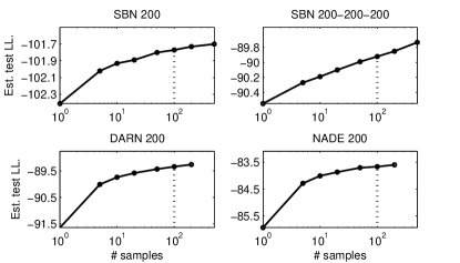
In Fig. 1, we investigate the influence of the number of samples $M$ on the posterior mean estimator Eqn. (19). We can observe that on all models using more samples for posterior mean brings consistent improvements. On SBN/SBN models using $M=100$ samples improves around $0.6$ nat than using $M=1$ (in which case one posterior sample is estimated). On autoregressive models, using $M=100$ samples brings an improvement more than $2$ nats.

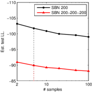
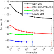
We show the influence of the number of samples $S$ used during training in Fig. 2. we observe that the Est. LL. on test data improves as $S$ grows up. Fig. 2 presents the curves of the final estimated test log-likelihood with respect to the number of samples $K$ used for the estimator Eqn. (20). We observe that $K=100,000$ and $K=500$ are large enough to get a good Est. LL. for SBN and DARN(NADE) models, respectively.

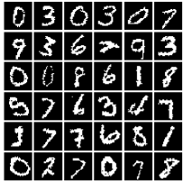
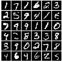
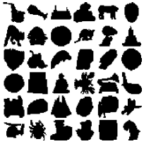
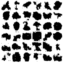
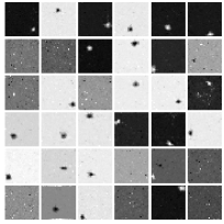
Fig. 3 visualizes the generative performance of the learned models. In Fig. 3, we show the randomly sampled training data of MNIST and Caltech 101 Silhouettes. Fig. 3 displays the examples generated from the learned models. We observe that the generated samples are visually good.

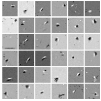
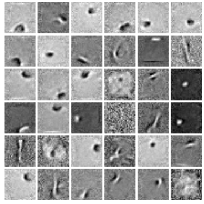
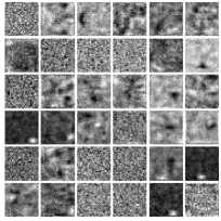
One advantage of Bayesian framework is that we can specify sparsity-encouraging priors on the model parameters explicitly, e.g., the Student-t prior in our experiments. Fig. 3 and Fig. 3 demonstrate the difference between features learned with a sparse (Student-t prior) prior and a non-sparse (Gaussian) prior. We observe that the features learned with a sparse prior appear more localized.

We further demonstrate the ability of the learned models on predicting missing data. For each test image, the lower half is assumed missing and the upper half is used to inference the hidden units (Gan et al., 2015b). Then, with the hidden units, the lower half is reconstructed. Prediction is done by repeating this procedure and finally sampling from the generative model with the inferred hidden units. Fig. 4 demonstrates some example completions for the missing data on MNIST.

Table 3: Caltech 101 Silhouettes results of various training methods and models. Results are taken from [1] Bornschein & Bengio (2015), [2] Cho et al. (2013), [3] Raiko et al. (2014). $\dagger$ Results are produced using the authors’ published code.

Methods (Models)	Est. test LL.
DSGNHT-NAIS (SBN/SBN 200)	$-122.7$
DSGNHT-NAIS (SBN/SBN 200-200)	$-108.0$
RWS (SBN/SBN 200)$\dagger$	$-134.4$
RWS (SBN/SBN 200-200)$\dagger$	$-126.0$
DSGNHT-NAIS (SBN/SBN 200-200-200)	$-105.2$
DSGNHT-NAIS (SBN/SBN 300-100-50-10)	$\mathbf{-103.6}$
DSGNHT-NAIS (NADE/NADE 150)	$\mathbf{-100.0}$
RWS (SBN/SBN 300-100-50-10) [1]	$-113.3$
RWS (NADE/NADE 150) [1]	$-104.3$
NADE (500 hidden units) [1]	$-110.6$
RBM (4000 hidden units) [2]	$-107.8$
NADE-5 (4000 hidden units) [3]	$-107.3$

4.2.2 Caltech 101 Silhouettes

The Caltech 101 Silhouettes dataset consists of $4,100$ training samples, $2,264$ validation samples and $2,307$ test samples. We first compare our method to RWS on two benchmark models in Table 3 (Top) and observe that our method achieves significant improvements. On SBN/SBN 200-200, we get a test Est. LL. of $-108.0$ which improves over RWS for $18$ nats.

Table 3 (Bottom) summarizes ours best results and other state-of-the-art results. Our NADE/NADE 150 network reaches a test Est. LL. of $-100.0$, which improves RWS on the same model for $4.3$ nats. We observe a remarkable effect of increasing the number of samples $M$ for posterior mean: the test Est. LL. of $-100.0$ at $M=100$ improves $5.3$ nats compared to $-105.3$ at $M=1$. Gan et al. (2015b) achieve $-96.40$ by training FVSBN (Frey, 1998) with both training data and validation data. A latest work by Goessling & Amit (2015) achieves $-88.48$ by developing a mixture model of sparse autoregressive network. Fig. 3 visualizes the samples drawn from the learned models.

Table 4: Results of log-likelihood estimation on single-stochastic-layer variational auto-encoder. Results of VAE and IWAE are taken from Burda et al. (2015).

Dataset	VAE	IWAE	DSGNHT-NAIS
binarized MNIST	$-88.83$	$-87.63$	$\mathbf{-86.93}$
Omniglot	$-107.62$	$-106.12$	$\mathbf{-106.10}$

4.3 Variational Auto-Encoders

Finally, we consider the DGMs with continuous hidden variables. One popular example is the variational auto-encoder (VAE) (Kingma & Welling, 2014). Intuitively, the posterior of DGMs with continuous hidden variables is harder to capture, as the hidden variables have much more freedom compared to that of DGMs with discrete hidden variables. Such freedom potentially results in high variance of the gradients estimation. VAE and the importance weighted auto-encoders (IWAE) (Burda et al., 2015) alleviate this problem by adopting a reparametrization trick. Then the variational parameters $\phi$ can be optimized tying to the generative model.

In our DSGNHT-NAIS, we indeed observe high variance of the gradients estimation. However in theory, any distribution that satisfies $q(\mathbf{z}|\mathbf{x};\bm{\phi})>0$ wherever $p(\mathbf{z}|\mathbf{x},\bm{\theta})>0$ can be used as a proposal. Such a property makes any other reasonable objectives (instead of the inclusive KL-divergence described in Sec. 3.3) for $q(\mathbf{z}|\mathbf{x};\bm{\phi})$ is adoptable. We adopt the same objective in IWAE for the proposal distribution and find it works well in practice.

We follow IWAE to train a single-stochastic-layer VAE with 50 hidden units. In between the data and the hidden variables are two deterministic layers with tanh activation. The model is trained on the binarized MNIST and the Omniglot datasets. We use the Omniglot dataset downloaded from Burda et al. (2015) which consists of $23,000$ training samples, $1,345$ validation samples and $87,00$ test samples. We use $M=200$ for the posterior mean estimator and follow IWAE to use $K=5,000$ to evaluate the test Est. LL.. Since IWAE also adopts an importance sampler to estimate the objective (as well as its gradient), we compare the results using $S=5$ samples during training for both IWAE and our method. We achieve comparable or better results as summarized in Table 4.

5 Conclusions and Future Work

We propose a powerful Bayesian inference method based on stochastic gradient MCMC for deep generative models with continuous parameter space. It enjoys several advantages of Bayesian formalism such as sparse Bayesian inference. Our results include state-of-the-art performance on standard published datasets.

For future work we like to investigate the performance on learning sparse Bayesian models. Also, learning nonparametric Bayesian DGMs is another interesting challenge.

Appendix A Model Setup

We describe how the models are constructed with the conditional stochastic layers. Each model should consists of a top layer $p(\mathbf{z}^{(L)}|\bm{\theta})$, a data layer $p(\mathbf{x}|\mathbf{z}^{(1)},\bm{\theta})$ and (optionally) several intermediate layer $p(\mathbf{z}^{(l)}|\mathbf{z}^{(1+1)},\bm{\theta})$. The output of the layer $(l+1)$ (random samples) is passed as the input to the layer $l$ and thus a full generative process for the data is built. In principle, the type of each layer can be chosen arbitrarily, as long as the input dimension and the output dimension of adjacent layers match to each other.

The recognition model can be constructed in a similar way. Given a generative model with $L$ hidden layers, the recognition model should also contains $L$ stochastic layers. The first layer takes $x$ as input and outputs random samples of $\mathbf{z}^{(1)}$. The output of the layer $l$ (random samples of $\mathbf{z}^{(l)}$) is passed as the input to the layer $l+1$. Note the type of each layer can also be chosen arbitrarily, as long as the dimensions of adjacent layers match to each other and the output dimension of the $l$-th layer matches the input dimension of the $l$-th layer of the generative model.

In our experiments, all tested models and their recognition models consist only one type of stochastic layer. In the following we describe the detailed architectures of our tested models.

SBN/SBN models:

For all models with SBN layers we construct the recognition model with SBN layers too. We use four SBN/SBN architectures in the experiments: 1-hidden-layer with 200 hidden units (SBN/SBN 200); 2-hidden-layer with 200 hidden units in each hidden layer (SBN/SBN 200-200); 3-hidden-layer with 200 hidden units in each hidden layer (SBN/SBN 200-200-200); and 4-hidden-layer with 300(closest to data), 100, 50, 10 hidden units (SBN/SBN 300-100-50-10).

We use the following top layer (equivalent to factorized Bernoulli distribution):

$$p(z^{(L)}_{i}=1|\bm{\theta})=\sigma(b_{i}),$$ (21)

and the likelihood model:

$$p(z^{(l)}_{i}=1|\mathbf{z}^{(l+1)},\bm{\theta})=\sigma(\mathbf{W}^{(l)}_{i,:}\mathbf{z}^{(l+1)}+b_{i}^{(l)}),$$ (22)

where we define $\mathbf{z}^{(0)}=\mathbf{x}$. The model parameters are $\bm{\theta}=\{\mathbf{W}^{(l)},\mathbf{b}^{(l)}\}_{l=0}^{L-1}\cup\{\mathbf{b}^{(L)}\}$.

DARN/NADE models:

we follow Bornschein & Bengio (2015) to use NADE layers in the recognition model for the DARN models. We test a shallow model (1-hidden-layer DARN/NADE 200) in our experiments. We use the following top layer (equivalent to FVSBN (Frey, 1998)):

$$p(z^{(L)}_{i}=1|\mathbf{z}^{(L)}_{<i},\bm{\theta})=\sigma(\mathbf{W}_{i,<i}^{(L)}\mathbf{z}^{(L)}_{<i}+b_{i}^{(L)}),$$ (23)

and the likelihood model:

$$p(z^{(l)}_{i} =1|\mathbf{z}^{(l)}_{<i},\mathbf{z}^{(l+1)},\bm{\theta})=$$ (24)

$$\sigma(\mathbf{U}_{i,:}^{(l)}\mathbf{z}^{(l+1)}+\mathbf{W}_{i,<i}^{(l)}\mathbf{z}^{(l)}_{<i}+b_{i}^{(l)}).$$

The model parameters are $\bm{\theta}=\{\mathbf{U}^{(l)}\}_{l=0}^{L-1}\cup\{\mathbf{W}^{(l)},\mathbf{b}^{(l)}\}_{l=0}^{L}$.

NADE/NADE models:

We test a shallow model (1-hidden-layer NADE/NADE 200) in our experiments. We use the following top layer:

$$p(z^{(L)}_{i}=1|\mathbf{z}^{(L)}_{<i},\bm{\theta})=$$ (25)

$$\sigma\Big{(}\mathbf{V}_{i,:}^{(L)}\sigma(\mathbf{W}_{:,<i}^{(L)} \mathbf{z}^{(L)}_{<i}+\mathbf{a}^{(L)})+b_{i}^{(L)}\Big{)},$$

and the likelihood model:

$$p(z^{(l)}_{i} =1|\mathbf{z}^{(l)}_{<i},\mathbf{z}^{(l+1)},\bm{\theta})=\sigma\Big{(}\mathbf{V}_{i,:}^{(l)}\sigma(\mathbf{W}_{:,<i}^{(l)}\mathbf{z}^{(l)}_{<i}$$

$$+ \mathbf{U}^{(l)}\mathbf{z}^{(l+1)}+\mathbf{a}^{(l)})+\mathbf{R}^{(l)}_{i,:}\mathbf{z}^{(l+1)}+b_{i}^{(l)}\Big{)},$$ (26)

The model parameters are $\bm{\theta}=\{\mathbf{U}^{(l)},\mathbf{R}^{(l)}\}_{l=0}^{L-1}\cup\{\mathbf{V}^{(l)},\mathbf{W}^{(l)},\mathbf{a}^{(l)},\mathbf{b}^{(l)}\}_{l=0}^{L}$.

Algorithm 2 A Detailed Version of Doubly Stochastic Gradient MCMC with Neural Adaptive Proposals

  Input: $\mathbf{X}=\{\mathbf{x}_{1},\cdots,\mathbf{x}_{N}\}$: the dataset

  Input: $S$: number of samples used during training

  Input: $M$: number of samples used for computing the posterior mean estimation Eqn. (19)

  Input: $\gamma$: per-batch learning rate for SGNHT, $|B|$: mini-batch size, $a$: momentum decay

  Input: $\eta^{\prime}$: step size for Adam

  Input: $n_{\bm{\theta}}$, $n_{\bm{\phi}}$: number of $\bm{\theta}$ or $\bm{\phi}$ update during each mini-batch

  Initialize $\bm{\theta}$, $\bm{\phi}$: following the heuristic of Glorot & Bengio (2010)

  Initialize $\mathbf{u}\sim\mathcal{N}(\bm{0},\eta\mathbf{I})$, $\bm{\alpha}=a\mathbf{I}$

  for epoch $=1,2,\cdots$ do

     Randomly split the data $\mathbf{X}$ into mini-batches $B_{1},\cdots,B_{N/|B|}$

     for mini-batch $B_{i}$ in $\{B_{1},\cdots,B_{N/|B|}\}$ do

        for $i_{\bm{\theta}}=1,\cdots,n_{\bm{\theta}}$ do

           Sample $\{\mathbf{z}_{n}^{(s)}\}_{s=1}^{S}$ from the proposal $q(\mathbf{z}|\mathbf{x}_{n};\bm{\phi})$, $n\in B_{i}$

           Estimate the gradients $\nabla\log p(\mathbf{x}_{n}|\bm{\theta})$ with Eqn. (14), $n\in B_{i}$

           Update $\bm{\theta}$ with Eqn. (29)

           for $i_{\bm{\phi}}=1,\cdots,n_{\bm{\phi}}$ do

              Sample $\{\mathbf{z}_{n}^{(s)}\}_{s=1}^{S}$ from the proposal $q(\mathbf{z}|\mathbf{x}_{n};\bm{\phi})$, $n\in B_{i}$

              Estimate the gradients $\nabla_{\bm{\phi}}\mathcal{J}(\bm{\phi};\bm{\theta},\mathbf{X})$ with Eqn. (18), $n\in B_{i}$

              Update $\bm{\phi}$ using Adam optimizer with $\nabla_{\bm{\phi}}\mathcal{J}(\bm{\phi};\bm{\theta},\mathbf{X})$

           end for

        end for

     end for

  end for

  Run another $M$ epochs to estimate the posterior mean $\hat{\bm{\theta}}$

  Output: $\hat{\bm{\theta}}$

VAE/VAE models:

For the VAE model, we follow Kingma & Welling (2014) to use an isotropic multivariate Gaussian top layer:

$$p(z^{(L)}_{i}=1|\bm{\theta})=\mathcal{N}(\bm{0},\mathbf{I}).$$ (27)

The VAE stochastic layer itself contains an internal MLP. In our experiments, we train single-stochastic-layer VAE with 50 hidden units. In between the data and the hidden variables are two deterministic layers with tanh activation. The dimension of the two deterministic layers are both 100. The recognition model is a stochastic VAE layer within which are two 100-dimensional deterministic layers. Such an architecture is used in Burda et al. (2015).

In experiments of training VAE, we adopt the objective in IWAE (Burda et al., 2015) for learning the proposal distribution $q(\mathbf{z}|\mathbf{x};\bm{\phi})$:

$$\mathcal{L}_{K}=\mathbb{E}_{\mathbf{z}^{(k)}\sim q(\mathbf{z}|\mathbf{x};\bm{\phi})}\left[\log\frac{1}{K}\sum_{k=1}^{K}\frac{p(\mathbf{x},\mathbf{z}^{(k)})}{q(\mathbf{z}^{(k)}|\mathbf{x})}\right].$$ (28)

Then the gradient can be evaluated by adopting the reparametrization trick (Kingma & Welling, 2014):

$$\nabla_{\bm{\phi}}\mathcal{L}_{K}= \nabla_{\bm{\phi}}\mathbb{E}_{\mathbf{z}^{(k)}\sim q(\mathbf{z}|\mathbf{x};\bm{\phi})}\left[\log\frac{1}{K}\sum\nolimits_{k=1}^{K}\frac{p(\mathbf{x},\mathbf{z}^{(k)})}{q(\mathbf{z}^{(k)}|\mathbf{x})}\right]$$

$$= \nabla_{\bm{\phi}}\mathbb{E}_{\bm{\epsilon}^{(k)}\sim p(\bm{\epsilon})}\left[\log\frac{1}{K}\sum\nolimits_{k=1}^{K}w(\mathbf{x},\mathbf{z}(\bm{\epsilon}^{(k)},\mathbf{x},\bm{\phi}))\right]$$

$$= \mathbb{E}_{\bm{\epsilon}^{(k)}\sim p(\bm{\epsilon})}\left[\nabla_{\bm{\phi}}\log\frac{1}{K}\sum\nolimits_{k=1}^{K}w(\mathbf{x},\mathbf{z}(\bm{\epsilon}^{(k)},\mathbf{x},\bm{\phi}))\right]$$

$$= \mathbb{E}_{\bm{\epsilon}^{(k)}\sim p(\bm{\epsilon})}\left[\sum\nolimits_{k=1}^{K}\widetilde{w_{k}}\nabla_{\bm{\phi}}\log w(\mathbf{x},\mathbf{z}(\bm{\epsilon}^{(k)},\mathbf{x},\bm{\phi}))\right],$$

where we have omitted the model parameters $\bm{\theta}$ in the above gradients, since $\bm{\theta}$ is fixed when learning the proposal distribution. In the above derivations, $\bm{\epsilon}^{(1)},\cdots,\bm{\epsilon}^{(K)}$ are the auxiliary variables as defined in VAE. $w_{k}=w(\mathbf{x},\mathbf{z}(\bm{\epsilon}^{(k)},\mathbf{x},\bm{\phi}))=\frac{p(\mathbf{x},\mathbf{z}(\bm{\epsilon}^{(k)},\mathbf{x},\bm{\phi}))}{q(\mathbf{z}(\bm{\epsilon}^{(k)},\mathbf{x},\bm{\phi})|\mathbf{x})}$ are the importance weight and $\widetilde{w_{i}}$ are the normalized importance weights as defined in IWAE.

Appendix B Experimental Setup

We describe our experimental setup here, including the parameter setting and implementation details.

In our implementation, we use the reformulated form of multivariate SGNHT (Ding et al., 2014):

$$\bm{\theta}_{t+1} =\bm{\theta}_{t}+\mathbf{u}_{t},$$ (29)

$$\mathbf{u}_{t+1} =\mathbf{u}_{t}-\bm{\xi}_{t}\odot\mathbf{u}_{t}-\eta\nabla_{\bm{\theta}}\tilde{U}(\bm{\theta}_{t+1})+\mathcal{N}(\bm{0},2a\eta\mathbf{I}),$$

$$\bm{\alpha}_{t+1} =\bm{\alpha}_{t}+(\mathbf{p}_{t+1}\odot\mathbf{p}_{t+1}-\eta\mathbf{I}),$$

where we have setting $\mathbf{u}=\lambda\mathbf{p}$, $\eta=\lambda^{2}$, $\bm{\alpha}=\lambda\bm{\xi}$ and $a=A\lambda$. This reformulation is cleaner and easier to implement. In analog to SGD with momentum, $\eta$ is called the learning rate and $\mathbf{1}-\bm{\alpha}$ are the momentum terms (Chen et al., 2014). The initialization of SGNHT is as follows: $\mathbf{u}$ is random sampled from $\mathcal{N}(\bm{0},\eta\mathbf{I})$ and $\bm{\alpha}$ is initialized as $a\mathbf{I}$. There are three parameters for SGNHT: the learning rate $\eta$, the momentum decay $a$, and the mini-batch size $B$. In our implementation we choose the mini-batch size $B=100$, the momentum decay $a=\{0.1,0.01\}$. For numerical stability, we choose $\eta=\frac{\gamma}{N}$, where $\gamma$ is called the “per-batch learning rate” (Chen et al., 2014). The per-batch learning rate $\gamma$ is chosen from $\{0.01,0.005,0.001\}$ with best performance.

For the recognition model, we use Adam (Kingma & Ba, 2015) to learn the parameters $\bm{\phi}$. There are four parameters for Adam: the stepsize $\eta^{\prime}$, the exponential decay rates $\{\beta_{1}$, $\beta_{2}\}$ and $\epsilon$ which is used to prevent division by zero. In our implementation we choose $\beta_{1}=0.9$, $\beta_{2}=0.999$ and $\epsilon=10^{-10}$. The stepsize $\eta^{\prime}$ is chosen from $\{1,3,5\}\times 10^{-4}$ with best performance.

The model parameters are initialized following the heuristic of Glorot & Bengio (2010). The Student-t’s prior for all model parameters are set with a scale parameter $\sigma=0.09$, location parameter $\mu=0$ and degrees of freedom $\nu=2.2$.

Our method involves updating the generative model parameters $\bm{\theta}$ and the recognition model parameters $\bm{\phi}$ together (one step of $\bm{\theta}$ update and one step of $\bm{\phi}$ update within each mini-batch). One natural extension is to make the numbers of the two type of updates adjustable. We thus set the parameter $n_{\bm{\theta}}$ which controls the number of steps of $\bm{\theta}$ update within each mini-batch, and parameter $n_{\bm{\phi}}$ which controls the number of steps of $\bm{\phi}$ update following each step of $\bm{\theta}$ update. Larger $n_{\bm{\theta}}$ can potentially make the samples of $\bm{\theta}$ less correlated. Larger $n_{\bm{\phi}}$ can potentially make the proposal distribution more accurate. We set $n_{\bm{\theta}}=10$ and $n_{\bm{\phi}}=1$ in our implementation.

Finally, in Alg. 2 we summarize a detailed version of our method.

Appendix C Derivations

We provide the derivations of the Gibbs sampler for the DSGNHT-Gibbs. The hidden variables are sampled layer-wisely and dimension-wisely. We define $\mathbf{z}^{(0)}=\mathbf{x}$ and $\mathbf{z}^{(L+1)}=\bm{0}$ for convenience. Then the probability $p(z^{(l)}_{i}|\mathbf{z}^{(l)}_{\neg i},\mathbf{x},\mathbf{z}^{(\neg l)})$ can be written as $p(z^{(l)}_{i}|\mathbf{z}^{(l)}_{\neg i},\mathbf{z}^{(\neg l)})$. We have the following Gibbs sampler:

$$p(z^{(l)}_{i}|\mathbf{z}^{(l)}_{\neg i},\mathbf{z}^{(\neg l)})$$

$$= p(z^{(l)}_{i}|\mathbf{z}^{(l)}_{\neg i},\mathbf{z}^{(<l)},\mathbf{z}^{(>l)})$$

$$\propto p(\mathbf{z}^{(<l)}|z^{(l)}_{i},\mathbf{z}^{(l)}_{\neg i},\mathbf{z}^{(>l)})\cdot p(z^{(l)}_{i}|\mathbf{z}^{(l)}_{\neg i},\mathbf{z}^{(>l)})$$

$$= p(\mathbf{z}^{(<l)}|\mathbf{z}^{(l)})\cdot p(z^{(l)}_{i}|\mathbf{z}^{(l+1)})$$

$$\propto p(\mathbf{z}^{(l-1)}|\mathbf{z}^{(l)})\cdot p(z^{(l)}_{i}|\mathbf{z}^{(l+1)})$$

$$= \!\!\prod_{i^{\prime}=1}^{D^{(l-1)}}\!\!\!\!\!\exp\!\biggl{[}(\mathbf{W}^{(l-1)^{\top}}_{i,:}\!\!\!\mathbf{z}^{(l)}\!+\!b^{(l)}_{i^{\prime}})z^{(l-1)}_{i^{\prime}}\!\!-\!\log(1\!+\!e^{(\mathbf{W}^{(l-1)^{\top}}_{i,:}\!\!\mathbf{z}^{(l)}\!+\!b^{(l)}_{i^{\prime}})})\biggr{]}$$

$$\times\!\!\exp\!\biggl{[}(\mathbf{W}^{(l)^{\top}}_{i,:}\!\!\!\mathbf{z}^{(l+1)}\!+\!b^{(l)}_{i})z^{(l)}_{i}\!\!-\!\!\log(1\!+\!e^{(\mathbf{W}^{(l-1)^{\top}}_{i,:}\!\!\!\mathbf{z}^{(l+1)}+b^{(l-1)}_{i})})\biggr{]}$$

$$\propto \exp\biggl{[}(\sum_{i^{\prime}=1}^{D^{(l-1)}}W^{(l-1)}_{i^{\prime}i}z^{(l-1)}_{i^{\prime}}+(\mathbf{W}^{(l)^{\top}}_{i,:}\mathbf{z}^{(l+1)}+b^{(l)}_{i}))z^{(l)}_{i}$$

$$\leavevmode\nobreak\ \leavevmode\nobreak\ \leavevmode\nobreak\ \leavevmode\nobreak\ \leavevmode\nobreak\ \leavevmode\nobreak\ \leavevmode\nobreak\ \leavevmode\nobreak\ \leavevmode\nobreak\ \leavevmode\nobreak\ \leavevmode\nobreak\ \leavevmode\nobreak\ \leavevmode\nobreak\ -\sum_{i^{\prime}=1}^{D^{(l-1)}}\log(1+e^{(\mathbf{W}^{(l-1)^{\top}}_{i^{\prime},:}\mathbf{z}^{(l)}+b^{(l)}_{i^{\prime}})})\biggr{]}.$$

A Gibbs sampler for DARN can be derived similarly.

References

- Adams et al. (2010) Adams, R., Wallach, H., and Ghahramani, Z. Learning the structure of deep sparse graphical models. In AISTATS, 2010.
- Ahn et al. (2012) Ahn, S., Korattikara, A., and Welling, M. Bayesian posterior sampling via stochastic gradient fisher scoring. In ICML, 2012.
- Bengio & Bengio (2000) Bengio, Y. and Bengio, S. Modeling high-dimensional discrete data with multi-layer neural networks. In NIPS, pp. 400–406. MIT Press, 2000.
- Bengio et al. (2014) Bengio, Y., Laufer, E., Alain, G., and Yosinski, J. Deep generative stochastic networks trainable by backprop. In ICML, 2014.
- Bornschein & Bengio (2015) Bornschein, J. and Bengio, Y. Reweighted wake-sleep. In ICLR, 2015.
- Bottou (1998) Bottou, L. Online Algorithms and Stochastic Approximations. Online Learning and Neural Networks, Edited by David Saad, Cambridge University Press, Cambridge, UK, 1998.
- Boulanger-Lewandowski et al. (2012) Boulanger-Lewandowski, N., Bengio, Y., and Vincent, P. Modeling temporal dependencies in high-dimensional sequences: Application to polyphonic music generation and transcription. In ICML, 2012.
- Burda et al. (2015) Burda, Y., Grosse, R. B., and Salakhutdinov, R. Importance weighted autoencoders. CoRR, abs/1509.00519, 2015.
- Chen et al. (2014) Chen, T., Fox, E., and Guestrin, C. Stochastic gradient hamiltonian monte carlo. In ICML, pp. 1683–1691, 2014.
- Cho et al. (2013) Cho, K., Raiko, T., and Ilin, A. Enhanced gradient for training restricted boltzmann machines. Neural computation, 25(3):805–831, 2013.
- Ding et al. (2014) Ding, N., Fang, Y., Babbush, R., Chen, C., Skeel, R., and Neven, H. Bayesian sampling using stochastic gradient thermostats. In NIPS, pp. 3203–3211, 2014.
- Frey (1998) Frey, B. J. Graphical models for machine learning and digital communication. 1998.
- Gan et al. (2015a) Gan, Z., Chen, C., Henao, R., Carlson, D., and Carin, L. Scalable deep poisson factor analysis for topic modeling. In ICML, 2015a.
- Gan et al. (2015b) Gan, Z., Henao, R., Carlson, D., and Carin, L. Learning deep sigmoid belief networks with data augmentation. In AISTATS, 2015b.
- Glorot & Bengio (2010) Glorot, X. and Bengio, Y. Understanding the difficulty of training deep feedforward neural networks. In AISTATS, pp. 249–256, 2010.
- Goessling & Amit (2015) Goessling, M. and Amit, Y. Sparse autoregressive networks. arXiv preprint arXiv:1511.04776, 2015.
- Gregor et al. (2014) Gregor, K., Danihelka, I., Mnih, A., Blundell, C., and Wierstra, D. Deep autoregressive networks. In ICML, 2014.
- Gregor et al. (2015) Gregor, K., Danihelka, I., Graves, A., Rezende, D., and Wierstra, D. Draw: A recurrent neural network for image generation. In ICML, pp. 1462–1471, 2015.
- Gu et al. (2015) Gu, S., Ghahramani, Z., and Turner, R. E. Neural adaptive sequential monte carlo. In NIPS, pp. 2611–2619, 2015.
- Hinton et al. (2006) Hinton, G. E., Osindero, S., and Teh, Y. A fast learning algorithm for deep belief nets. Neural Computation, 18, 2006.
- Jordan et al. (1999) Jordan, M., Ghahramani, Z., Jaakkola, T., and Saul, L. An introduction to variational methods for graphical models. MLJ, 37(2):183–233, 1999.
- Kingma & Ba (2015) Kingma, D. P. and Ba, J. L. Adam: A method for stochastic optimization. In ICLR, 2015.
- Kingma & Welling (2014) Kingma, D. P. and Welling, M. Auto-encoding variational Bayes. In ICLR, 2014.
- Lake et al. (2013) Lake, B. M., Salakhutdinov, R., and Tenenbaum, J. One-shot learning by inverting a compositional causal process. In NIPS, pp. 2526–2534, 2013.
- Larochelle & Murray (2011) Larochelle, H. and Murray, I. The neural autoregressive distribution estimator. In AISTATS, 2011.
- Lecun et al. (1998) Lecun, Y., Bottou, L., Bengio, Y., and Haffner, P. Gradient-based learning applied to document recognition. Proceedings of the IEEE, 86(11):2278–2324, 1998.
- Li et al. (2016) Li, C., Chen, C., Fan, K., and Carin, L. High-order stochastic gradient thermostats for bayesian learning of deep models. In AAAI, 2016.
- MacKay (1992) MacKay, D. A practical bayesian framework for backpropagation networks. Neural Computation, 4(3):448–472, 1992.
- Marlin et al. (2010) Marlin, B., Swersky, K., Chen, B., and Freitas, N. Inductive principles for restricted boltzmann machine learning. In AISTATS, pp. 509–516, 2010.
- Mnih & Gregor (2014) Mnih, A. and Gregor, K. Neural variational inference and learning in belief networks. In ICML, 2014.
- Murray & Salakhutdinov (2009) Murray, I. and Salakhutdinov, R. Evaluating probabilities under high-dimensional latent variable models. In NIPS, pp. 1137–1144, 2009.
- Neal (1992) Neal, R. M. Connectionist learning of belief networks. Artificial intelligence, 56(1):71–113, 1992.
- Neal (1995) Neal, R. M. Bayesian learning for neural networks. PhD thesis, University of Toronto, 1995.
- Owen (2013) Owen, A. B. Monte Carlo theory, methods and examples. 2013.
- Raiko et al. (2014) Raiko, T., Li, Y., Cho, K., and Bengio, Y. Iterative neural autoregressive distribution estimator nade-k. In NIPS, pp. 325–333, 2014.
- Ranganath et al. (2014) Ranganath, R., Gerrish, S., and Blei, D. M. Black box variational inference. In ICML, 2014.
- Rezende et al. (2014) Rezende, D. J., Mohamed, S., and Wierstra, D. Stochastic backpropagation and approximate inference in deep generative models. In ICML, 2014.
- Robbins & Monro (1951) Robbins, H. and Monro, S. A stochastic approximation method. The Annals of Mathematical Statistics, 22(3):400–4007, 1951.
- Robert & Casella (2005) Robert, C. and Casella, G. Monte Carlo Statistical Methods. Springer, 2005.
- Salakhutdinov & Hinton (2009) Salakhutdinov, R. and Hinton, G. E. Deep Boltzmann machines. In AISTATS, 2009.
- Salakhutdinov & Murray (2008) Salakhutdinov, R. and Murray, I. On the quantitative analysis of deep belief networks. In ICML, pp. 872–879, 2008.
- Saul et al. (1996) Saul, L., Jaakkola, T., and Jordan, M. Mean field theory for sigmoid belief networks. Journal of AI Research, 4:61–76, 1996.
- Titsias & Lázaro-Gredilla (2014) Titsias, M. K. and Lázaro-Gredilla, M. Doubly stochastic variational bayes for non-conjugate inference. In ICML, pp. 1971–1979, 2014.
- Uria et al. (2014) Uria, B., Murray, I., and Larochelle, H. A deep and tractable density estimator. In ICML, pp. 467–475, 2014.
- Welling & Teh (2011) Welling, M. and Teh, Y. W. Bayesian learning via stochastic gradient Langevin dynamics. In ICML, 2011.