Few-second-long correlation times in a quantum dot nuclear spin bath probed by frequency-comb NMR spectroscopy

One of the key challenges in spectroscopy is inhomogeneous broadening that masks the homogeneous spectral lineshape and the underlying coherent dynamics. A variety of techniques including four-wave mixing and spectral hole-burning are used in optical spectroscopy ^{1, 2, 3} while in nuclear magnetic resonance (NMR) spin-echo ⁴ is the most common way to counteract inhomogeneity. However, the high-power pulses used in spin-echo and other sequences ^{4, 5, 6, 7, 8} often create spurious dynamics ^{7, 8} obscuring the subtle spin correlations that play a crucial role in quantum information applications ^{5, 6, 9, 10, 11, 12, 13, 14, 15, 16, 17}. Here we develop NMR techniques that allow the correlation times of the fluctuations in a nuclear spin bath of individual quantum dots to be probed. This is achieved with the use of frequency comb excitation which allows the homogeneous NMR lineshapes to be measured avoiding high-power pulses. We find nuclear spin correlation times exceeding 1 s in self-assembled InGaAs quantum dots - four orders of magnitude longer than in strain-free III-V semiconductors. The observed freezing of the nuclear spin fluctuations opens the way for the design of quantum dot spin qubits with a well-understood, highly stable nuclear spin bath.

Pulsed magnetic resonance is a diverse toolkit with applications in chemistry, biology and physics. In quantum information applications, solid state spin qubits are of great interest and are often described by the so called central spin model, where the qubit (central spin) is coupled to a fluctuating spin bath (typically interacting nuclear spins). Here microwave and radio-frequency (rf) magnetic resonance pulses are used for the initialization and readout of a qubit ¹⁸, dynamic decoupling ⁵ and dynamic control ⁶ of the spin bath.

However, the most important parameter controlling the central spin coherence ^{19, 9, 11} - the correlation time $\tau_{\textrm{c}}$ of the spin bath fluctuations is very difficult to measure directly. The $\tau_{\textrm{c}}$ is determined by the spin exchange (flip-flops) of the interacting nuclear bath spins. By contrast pulsed NMR reveals the spin bath coherence time $T_{2}$, which characterizes the dynamics of the transverse nuclear magnetization ^{7, 8, 2} and is much shorter than $\tau_{\textrm{c}}$. The problem is further exacerbated in self-assembled quantum dots where quadrupolar effects lead to inhomogeneous NMR broadening exceeding 10 MHz (Refs. ^{1, 22}), making rf field amplitudes required for pulsed NMR practically unattainable.

Here we develop an alternative approach to NMR spectroscopy: we measure non-coherent depolarisation of nuclear spins under weak noise-like rf fields. Contrary to intuitive expectation, we show that such measurement can reveal the full homogeneous NMR lineshape describing the coherent spin dynamics. This is achieved when rf excitation has a frequency comb profile (widely used in precision optical metrology ²³). We then exploit non-resonant nuclear-nuclear interactions: the homogeneous NMR lineshape of one isotope measured with frequency comb NMR is used as a sensitive non-invasive probe of the correlation times $\tau_{\textrm{c}}$ of the nuclear flip-flops of the other isotope. While initial studies ^{19, 9, 17} suggested $\tau_{\textrm{c}}\sim 100~{}\mu$s for nuclear spins in III-V semiconductors, it was recently recognized ^{24, 2, 9} that quadrupolar effects may have a significant impact in self-assembled quantum dots. Here we for the first time obtain a quantitative measurement of extremely long $\tau_{\textrm{c}}\gtrsim 1~{}$s revealing strong freezing of the nuclear spin bath - a crucial advantage for quantum information applications of self-assembled quantum dots.

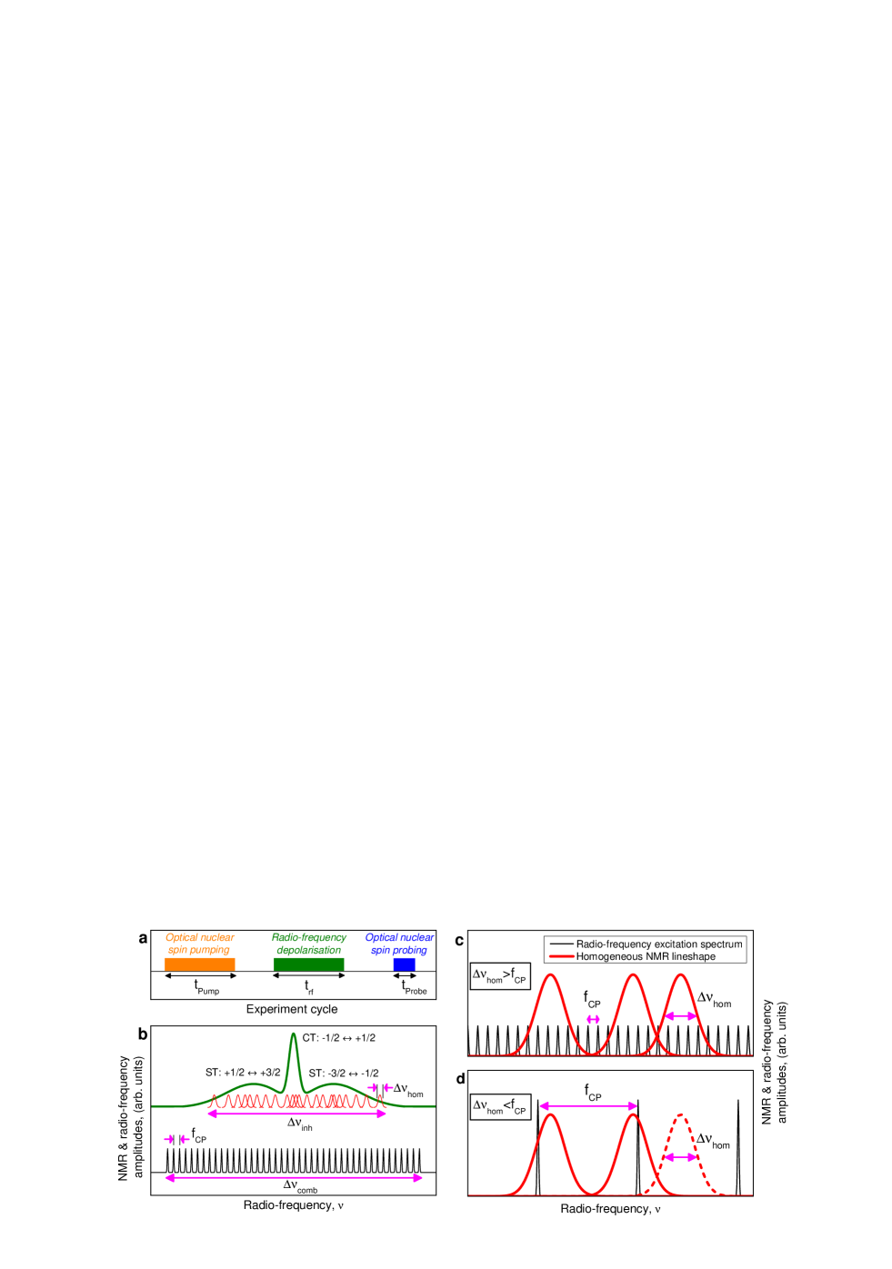
Figure 1: Frequency-comb technique for homogeneous NMR lineshape measurement. a, Timing diagram of the experimental cycle consisting of nuclear spin optical pumping (duration $t_{\textrm{Pump}}$), frequency-comb rf excitation ($t_{\textrm{rf}}$), and optical probing of the the nuclear spin state ($t_{\textrm{Probe}}$). b, The green line shows schematically a quantum dot NMR spectrum consisting of a central transition (CT) peak and two satellite transition (ST) bands. The inhomogeneous lineshape (width $\Delta\nu_{\textrm{inh}}$) is a sum of a large number ($>$1000) of nuclear spin transitions with homogeneous linewidths $\Delta\nu_{\textrm{hom}}$ (shown with red lines). The thin black line shows the spectrum of the frequency-comb excitation with comb period $f_{\textrm{CP}}$ and total width $\Delta\nu_{\textrm{comb}}$ exceeding $\Delta\nu_{\textrm{inh}}$. c, and d, demonstrate how experiments with varying $f_{\textrm{CP}}$ can reveal the width $\Delta\nu_{\textrm{hom}}$ of the NMR homogeneous lineshape (red lines). When $\Delta\nu_{\textrm{hom}}>f_{\textrm{CP}}$ (c) all individual nuclei are uniformly excited by the frequency comb (shown with black lines). In the opposite case $\Delta\nu_{\textrm{hom}}<f_{\textrm{CP}}$ (d) some of the nuclei (dashed line) are not excited resulting in a slow-down of nuclear spin dynamics. The transition between the two cases takes place when $f_{\textrm{CP}}\sim\Delta\nu_{\textrm{hom}}$, allowing $\Delta\nu_{\textrm{hom}}$ to be measured.

The experiments were performed on individual neutral self-assembled InGaAs/GaAs quantum dots at magnetic field $B_{\textrm{z}}=8$ T. All measurements of the nuclear spin depolarisation dynamics employ the pump-depolarise-probe protocol shown in Fig. 1a. Here we exploit the hyperfine interaction of the nuclei with the optically excited electron ^{17, 1, 22} both to polarise the nuclei (pump pulse) and to measure the nuclear spin polarisation in terms of the Overhauser shift $\Delta E_{\textrm{hf}}$ in the QD photoluminescence spectrum (probe pulse). The rf magnetic field depolarising nuclear spins is induced by a small copper coil. (Further experimental details can be found in Methods and Supplementary Note 1.)

All isotopes in the studied dots possess non-zero quadrupolar moments. Here we focus on the spin $I=3/2$ nuclei ⁷¹Ga and ⁷⁵As. The strain-induced quadrupolar shifts result in an inhomogeneously broadened NMR spectrum ^{1, 22} as shown schematically by the green line in Fig. 1b. The spectrum consists of a central transition (CT) $-1/2\leftrightarrow+1/2$ and two satellite transition (ST) $\pm 1/2\leftrightarrow\pm 3/2$ peaks. The NMR spectrum with inhomogeneous linewidth $\Delta\nu_{\textrm{inh}}$ consists of individual nuclear spin transitions (shown with red lines) with much smaller homogeneous linewidth $\Delta\nu_{\textrm{hom}}$.

To make a non-coherent depolarisation experiment sensitive to the homogeneous NMR lineshape rf excitation with a frequency comb spectral profile is used. As shown in Fig. 1b (black line) the frequency comb has a period of $f_{\textrm{CP}}$ and a total comb width $\Delta\nu_{\textrm{comb}}$ exceeding $\Delta\nu_{\textrm{inh}}$. The key idea of the frequency comb technique is described in Figs. 1c and d where two possible cases are shown. If the comb period is small ($f_{\textrm{CP}}<\Delta\nu_{\textrm{hom}}$, Fig. 1c) all nuclear transitions are excited by a large number of rf modes. As a result all nuclear spins are depolarised at the same rate and we expect an exponential decay of the total nuclear spin polarisation. In the opposite case of large comb period ($f_{\textrm{CP}}>\Delta\nu_{\textrm{hom}}$, Fig. 1d) some of the nuclear transitions are out of resonance and are not excited (e.g. the one shown by the dashed red line). As a result we expect a slowed-down non-exponential nuclear depolarisation. The experiments are performed at different $f_{\textrm{CP}}$; the $f_{\textrm{CP}}$ for which a slow-down in depolarisation is observed gives a measure of the homogeneous linewidth $\nu_{\textrm{hom}}$.

Experimental demonstration of this technique is shown in Fig. 2a. The Overhauser shift variation $\Delta E_{\textrm{hf}}$ of ⁷¹Ga is shown as a function of the depolarising rf pulse duration $t_{\textrm{rf}}$ for different $f_{\textrm{CP}}$. For small $f_{\textrm{CP}}=$80 and 435 Hz an exponential depolarisation is observed. However, when $f_{\textrm{CP}}$ is increased the depolarisation becomes non-exponential and slows down dramatically. The detailed dependence $\Delta E_{\textrm{hf}}(t_{\textrm{rf}},f_{\textrm{CP}})$ is shown as a colour-coded plot in Fig. 2b. The threshold value of $f_{\textrm{CP}}$ (marked with a white arrow) above which the nuclear spin dynamics becomes sensitive to the discrete structure of the frequency comb, provides an estimate of $\Delta\nu_{\textrm{hom}}\sim$ 450 Hz. Such a small homogeneous linewidth is detected in NMR resonances with inhomogeneous broadening of $\Delta\nu_{\textrm{inh}}\sim 6$ MHz (Ref. ¹) demonstrating the resolution power of frequency-comb non-coherent spectroscopy.

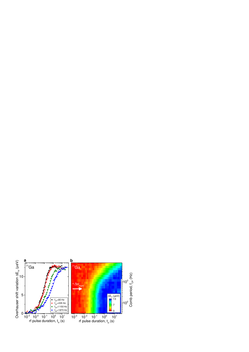
Figure 2: Measurement of the homogeneous NMR lineshape in self-assembled quantum dots using frequency-comb excitation. a, The change in the polarisation of the ⁷¹Ga nuclear spins (measured in terms of the change in the Overhauser shift $\Delta E_{\textrm{hf}}$) is shown as a function of the rf pulse duration $t_{\textrm{rf}}$ (symbols) at $B_{\textrm{z}}=8$ T and different comb periods $f_{\textrm{CP}}$. Lines show model fitting (see text). b, A full 2D plot of $\Delta E_{\textrm{hf}}$ as a function of $t_{\textrm{RF}}$ and $f_{\textrm{CP}}$ in the same experiment as in a. There is a clear slow-down of the nuclear spin depolarisation at $f_{\textrm{CP}}>450$ Hz (shown with a white arrow) providing an estimate of the homogeneous linewidth of $\Delta\nu_{\textrm{hom}}$.

The information revealed by frequency-comb spectroscopy is not limited to linewidth estimates. An accurate determination of the full homogeneous lineshape is achieved with modeling based on solving an integral equation (see details in Methods and Supplementary Note 2). We use the following two-parameter phenomenological model for the homogeneous lineshape:

$$\begin{aligned} &L(\nu)\propto\left(1+4(\sqrt[k]{2}-1)\frac{\nu^{2}}{\Delta\nu_{\textrm{hom}}^{2}}\right)^{-k},\end{aligned}$$ (1)

where $\Delta\nu_{\textrm{hom}}$ is the homogeneous full width at half maximum and $k$ is a roll-off parameter that controls the tails of the lineshape (the behavior of $L(\nu)$ at large $\nu$). For $k=1$ the lineshape corresponds to Lorentzian, while for $k\rightarrow\infty$ it tends to Gaussian: in this way Eq. 1 seamlessly describes the two most common lineshapes. Using $\Delta\nu_{\textrm{hom}}$ and $k$ as parameters we calculate the model $\Delta E_{\textrm{hf}}(t_{\textrm{rf}},f_{\textrm{CP}})$ dependence and fit it to the experimental $\Delta E_{\textrm{hf}}(t_{\textrm{rf}},f_{\textrm{CP}})$ to find an accurate phenomenological description of the homogeneous NMR lineshape in self-assembled quantum dots.

The solid line in Fig. 3a shows the best-fit lineshape ($\Delta\nu_{\textrm{hom}}\approx 221$ Hz and $k\approx 1.67$) for the measurement shown in Figs. 2a, b. The dashed and dashed-dotted lines in Fig. 3a show for comparison the Lorentzian ($k=1$) and Gaussian ($k\rightarrow\infty$) lineshapes with the same $\Delta\nu_{\textrm{hom}}$. The difference in the lineshape tails is seen clearly in Fig. 3b where a logarithmic scale is used. The model $\Delta E_{\textrm{hf}}(t_{\textrm{rf}},f_{\textrm{CP}})$ dependence calculated with the best fit parameters is shown in Fig. 3c and with lines in Fig. 2a - there is excellent agreement with experiment. By contrast modelling $\Delta E_{\textrm{hf}}(t_{\textrm{rf}},f_{\textrm{CP}})$ with Lorentzian (Fig. 3d) and Gaussian (Fig. 3e) lineshapes show a pronounced deviation from the experiment, demonstrating the excellent sensitivity of the frequency-comb spectroscopy to accurately probe the homogeneous spectral lineshape.

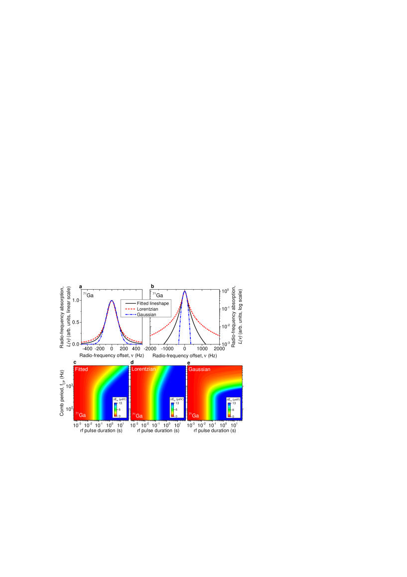
Figure 3: Homogeneous lineshape modeling. a, b, Model homogeneous NMR lineshapes of ⁷¹Ga nuclei shown on linear (a) and logarithmic (b) scale. Solid lines show the best-fit lineshape with a full width at half maximum $\Delta\nu_{\textrm{hom}}\approx 221$ Hz and a roll-off parameter $k\approx 1.67$. Dashed and dashed-dotted lines show for comparison Lorentzian and Gaussian lineshapes with the same $\Delta\nu_{\textrm{hom}}$. c-e, The calculated $\Delta E_{\textrm{hf}}(t_{\textrm{rf}},f_{\textrm{CP}})$ dependencies for the lineshapes in (a, b). For the fitted lineshape (c) an excellent agreement with the experiment in Fig. 2b is found, while calculations with Lorentzian (d) and Gaussian (e) lineshapes give markedly different results demonstrating the sensitivity of the frequency comb technique.

We have also performed frequency comb NMR spectroscopy on ⁷⁵As nuclei (Fig. 4a). Despite their larger inhomogeneous broadening $\Delta\nu_{\textrm{inh}}\sim 18$ MHz the model fitting reveals even smaller $\Delta\nu_{\textrm{hom}}\approx 117$ Hz and $k\approx 1.78$. The frequency-comb measurements are in agreement with the previous findings based on spin-echo NMR measurements ²: indeed, from $\Delta\nu_{\textrm{hom}}$ derived here we can estimate the nuclear spin coherence time $T_{2}\approx 1/(\pi\Delta\nu_{\textrm{hom}})\sim 1.4$ and $2.7$ ms for ⁷¹Ga and ⁷⁵As, in good agreement with the corresponding spin-echo $T_{2}\approx 1.2$ and $4.3~{}$ms. On the other hand, spin-echo could only be measured on central transitions for which $\Delta\nu_{\textrm{inh}}$ is relatively small. Moreover pulsed NMR does not allow determination of the full homogeneous lineshape, which for dipole-dipole interactions typically has a ”top-hat”-like (Guassian) profile ²⁶. And most importantly, due to the parasitic effects such as ”instantaneous diffusion” ⁷ and spin locking ⁸ pulsed NMR does not reveal the characteristic correlation time $\tau_{\textrm{c}}$ of the spin exchange (spin flip-flop) between the nuclei in the absence of rf excitation.

As we now show, the non-Gaussian lineshapes can be understood and $\tau_{\textrm{c}}$ can be derived using experiments with two frequency combs exciting nuclei of two isotopes (⁷⁵As and ⁷¹Ga). The two-comb experiment is similar to that shown in Fig. 4a: we excite ⁷⁵As nuclei with a frequency comb to measure their homogeneous lineshape. The difference is that now we simultaneously apply a second comb exciting the ⁷¹Ga spins. Importantly, in this experiment the ⁷¹Ga nuclei are first fully depolarised after the optical nuclear spin pumping – in this way the excitation of ⁷¹Ga has no direct effect on the measured hyperfine shift $\Delta E_{\textrm{hf}}$. By contrast it leads to ”heating” of the ⁷¹Ga spins which has only an indirect effect on $\Delta E_{\textrm{hf}}$ by changing the ⁷⁵As lineshape via dipolar coupling between ⁷¹Ga and ⁷⁵As spins. The result of the two-comb experiment is shown in Fig. 4b: a clear increase of $\Delta\nu_{\textrm{hom}}$ for ⁷⁵As is observed. From model fitting we find that ⁷¹Ga ”heating” leads to a 3 times broader homogeneous linewidth $\Delta\nu_{\textrm{hom}}\approx 355$ Hz of ⁷⁵As and its homogeneous lineshape is modified towards Gaussian, observed as increased $k\approx 2.32$.

Figure 4: Probing the correlation times of the nuclear spin bath fluctuation. a, b, Frequency-comb measurement on ⁷⁵As nuclei at $B_{\textrm{z}}=$8 T without (a) and with (b) additional frequency-comb excitation ”heating” the ⁷¹Ga nuclei. The increase of $\Delta\nu_{\textrm{hom}}$ of ⁷⁵As under the ⁷¹Ga ”heating” reveals the strongly suppressed nuclear spin fluctuations of ⁷¹Ga. c, rf-induced depolarisation time $\tau_{\textrm{As}}$ of ⁷⁵As nuclei at fixed $f_{\textrm{CP}}=1.47$ kHz as a function of the amplitude $\beta_{1}$ of the addition rf excitation ”heating” either the central transition (CT, triangles) or the satellite transition (ST, squares) of ⁷¹Ga. The bottom scale shows $\beta_{1}$ expressed in terms of the rf-induced spin-flip time $\tau_{\textrm{Ga}}$ of ⁷¹Ga. The $\tau_{\textrm{Ga}}$ at which a marked decrease of $\tau_{\textrm{As}}$ is observed corresponds to the correlation time $\tau_{\textrm{c}}$ of the ⁷¹Ga nuclear spin fluctuations: By extrapolating the power-law regions (dashed lines) to the intersection with the maximum $\tau_{\textrm{As}}$ (solid line) we deduce $\tau_{\textrm{c,CT}}\approx 1$ sec and $\tau_{\textrm{c,ST}}\approx 20$ sec for the CT and ST transitions.

To explain this result we note that the NMR lineshape is a statistical distribution of NMR frequency shifts of each nucleus produced by its dipolar interaction with all possible configurations of the neighboring nuclear spins. However, the frequency comb experiment is limited in time (up to $\sim$100 s as shown in Figs. 4a, b). If the nuclear spin environment of each ⁷⁵As nucleus does not go through all possible configurations during the measurement time, the frequency shifts are effectively static, and hence are eliminated from the lineshape as for any other inhomogeneous broadening.

Thus we conclude that the narrowed, non-Gaussian ($k\approx$1.6–1.8) homogeneous NMR lineshape arises from the ”snapshot” nature of the frequency comb measurement, probing the strongly frozen nuclear spin configuration. When the additional ⁷¹Ga ”heating” excitation is applied it ”thaws” the ⁷¹Ga spins, detected as broadening of the ⁷⁵As lineshape (as demonstrated in Figs. 4a, b). We use such sensitivity of the ⁷⁵As lineshape to measure the dynamics of the ⁷¹Ga equilibrium spin bath fluctuations. Based on the results of Fig. 4 the ⁷⁵As spins are now excited with a frequency comb with a fixed $f_{\textrm{CP}}=1.47$ kHz for which the ⁷⁵As depolarisation dynamics is most sensitive to the ⁷¹Ga ”heating”. Furthermore, we now use selective ”heating” of either the $-1/2\leftrightarrow+1/2$ CT or the $+1/2\leftrightarrow+3/2$ ST of ⁷¹Ga. The amplitude $\beta_{1}$ of the ”heating” frequency comb is varied – the resulting dependencies of the ⁷⁵As depolarisation time $\tau_{\textrm{As}}$ are shown in Fig. 4c by the squares and triangles for CT and ST ”heating” respectively. For analysis we also express $\beta_{1}$ in terms of the rf-induced ⁷¹Ga spin-flip time $\tau_{\textrm{Ga}}$ (bottom scale in Fig. 4c, see details in Methods).

It can be seen that for vanishing ⁷¹Ga excitation ($\beta\rightarrow 0$) the ⁷⁵As depolarisation time $\tau_{\textrm{As}}$ is constant. In this ”frozen” regime the rf-induced spin-flip time $\tau_{\textrm{Ga}}$ of ⁷¹Ga is larger than the correlation time $\tau_{\textrm{c}}$ of the ⁷¹Ga intrinsic spin flip-flops ($\tau_{\textrm{Ga}}>\tau_{\textrm{c}}$). As a result $\tau_{\textrm{As}}$ is determined only by the rf excitation of ⁷⁵As itself. However, when $\beta_{1}$ is increased to $\sim$1–10 nT Hz^-1/2 the rf induced spin-flips of ⁷¹Ga nuclei become faster than their intrinsic flip-flops ($\tau_{\textrm{Ga}}<\tau_{\textrm{c}}$). Such ”thawing” of ⁷¹Ga broadens the ⁷⁵As lineshape (via heteronuclear interaction), and is observed as a reduction of $\tau_{\textrm{As}}$. Thus the transition from the ”frozen” to ”thawed” regimes takes place when $\tau_{\textrm{Ga}}\approx\tau_{\textrm{c}}$, allowing $\tau_{\textrm{c}}$ to be determined. In Fig. 4c we extrapolate graphically (dashed lines) the power-law dependence in the ”thawed” regime. The points of the intersections with the limiting value of $\tau_{\textrm{As}}$ in the ”frozen” regime (solid horizontal line) yield correlation times $\tau_{\textrm{c,CT}}\sim 1$ s for CT and $\tau_{\textrm{c,ST}}\sim 20$ s for ST.

The observed $\tau_{\textrm{c}}\gtrsim 1$ s exceeds very strongly typical nuclear dipolar flip-flop times in strain-free III-V solids $\tau_{\textrm{c}}\sim 100~{}\mu$s ^{10, 9, 17}. We attribute the extremely long $\tau_{\textrm{c}}$ in self-assembled quantum dots to the effect of inhomogeneous nuclear quadrupolar shifts making nuclear spin flip-flops energetically forbidden ^{24, 2}. This interpretation is corroborated by the observation of $\tau_{\textrm{c,ST}}\gg\tau_{\textrm{c,CT}}$, since quadrupolar broadening of the ST transitions is much larger than that of the CT ¹. Furthermore, the ⁷¹Ga spins examined here have the largest gyromagnetic ratio $\gamma$ and the smallest quadrupolar moment $Q$, so we expect that all other isotopes in InGaAs have even longer $\tau_{\textrm{c}}$, resulting in the overall $\tau_{\textrm{c}}\gtrsim 1$ s of the entire quantum dot nuclear spin bath. This implies that in high magnetic fields the spin-echo coherence times of the electron and hole spin qubits in self-assembled dots are not limited by the nuclear spin bath up to sub-second regimes ^{10, 27, 9, 12}. Provided that other mechanisms of central spin dephasing, such as charge fluctuations ^{13, 14, 15} are eliminated, this would open the way for optically active spin qubit networks in III-V semiconductors with coherence properties previously achievable only in nuclear-spin-free materials ^{28, 29}.

Since the frequency-comb technique is not limited by artifacts in the spin dynamics hampering pulsed magnetic resonance, it allows detection of very slow spin bath fluctuations. Such sensitivity of the method can be used for example to investigate directly the effect of the electron or hole on the spin bath fluctuations in charged quantum dots, arising for example from hyperfine-mediated nuclear spin interactions. The experiments can be well understood within a classical rate equation model, while further advances in frequency comb spectroscopy can be expected with the development of a full quantum mechanical model. Furthermore, the simple and powerful ideas of frequency-comb NMR spectroscopy can be readily extended beyond quantum dots: as we show in Supplementary Note 3 the only essential requirement is that the longitudinal relaxation time $T_{1}$ should be larger (by about two orders of magnitude) than the transverse relaxation time $T_{2}$, which is usually the case in solid state spin systems. Finally our approaches in the use of frequency combs can go beyond NMR, and for example enrich the techniques in optical spectroscopy.

I Methods Summary

Sample structures and experimental techniques The experiments were performed on individual neutral self-assembled InGaAs/GaAs quantum dots. The sample was mounted in a helium-bath cryostat ($T$=4.2 K) with a magnetic field $B_{\textrm{z}}=8$ T applied in the Faraday configuration (along the sample growth and light propagation direction $Oz$). Radio-frequency (rf) magnetic field $B_{\textrm{rf}}$ perpendicular to $B_{\textrm{z}}$ was induced by a miniature copper coil. Optical excitation was used to induce nuclear spin magnetization exceeding 50%, as well as to probe it by measuring hyperfine shifts in photoluminescence spectroscopy¹.

Two sample structures have been studied, both containing a single layer of InGaAs/GaAs quantum dots embedded in a weak planar microcavity with a Q-factor of $\sim$250. In one of the samples the dots emitting at $\sim 945$ nm were placed in a $p-i-n$ structure, where application of a large reverse bias during the rf excitation ensured the neutral state of the dots. The results for this sample are shown in Fig. 2. The second sample was a gate-free structure, where most of the dots emitting at $\sim 914$ nm are found in a neutral state, although the charging can not be controlled. Excellent agreement between the lineshapes of both ⁷¹Ga and ⁷⁵As in the two structures was found, confirming the reproducibility of the frequency-comb technique.

Homogeneous lineshape theoretical model. Let us consider an ensemble of spin $I=1/2$ nuclei with gyromagnetic ratio $\gamma$ and inhomogeneously broadened distribution of nuclear resonant frequencies $\nu_{\textrm{nuc}}$. We assume that each nucleus has a homogeneous absorption lineshape $L(\nu)$, with normalization $\int_{-\infty}^{+\infty}L(\nu)d\nu=1$. A small amplitude (non-saturating) rf field will result in depolarisation, which can be described by a differential equation for population probabilities $p_{\pm 1/2}$ of the nuclear spin levels $I_{\textrm{z}}=\pm 1/2$

$$d(p_{+1/2}-p_{-1/2})/dt=-W(p_{+1/2}-p_{-1/2}).$$ (2)

For frequency-comb excitation the decay rate is the sum of the decay rates caused by each rf mode with magnetic field amplitude $B_{\textrm{1}}$, and can be written as:

$$W(\nu_{\textrm{nuc}})=\frac{\gamma^{2}B_{\textrm{1}}^{2}}{2f_{\textrm{CP}}}\sum_{j=0}^{N_{\textrm{m}}-1}L(\nu_{\textrm{nuc}}-\nu_{1}-jf_{\textrm{CP}})f_{\textrm{CP}},$$ (3)

where the summation goes over all modes with frequencies $\nu_{\textrm{j}}=\nu_{\textrm{1}}+jf_{\textrm{CP}}$ ($\nu_{\textrm{1}}$ is the frequency of the first spectral mode).

The change in the Overhauser shift $E_{\textrm{hf}}$ produced by each nucleus is proportional to $p_{+1/2}-p_{-1/2}$ and according to Eq. 2 has an exponential time dependence $\propto\exp(-W(\nu_{\textrm{nuc}})t)$. The quantum dot contains a large number of nuclear spins with randomly distributed absorption frequencies. Therefore to obtain the dynamics of the total Overhauser shift we need to average over $\nu_{\textrm{nuc}}$, which can be done over one period $f_{\textrm{CP}}$ since the spectrum of the rf excitation is periodic. Furthermore, since the total width of the rf frequency comb $\Delta\nu_{\textrm{comb}}$ is much larger than $f_{\textrm{CP}}$ and $\Delta\nu_{\textrm{hom}}$, the summation in Eq. 3 can be extended to $\pm\infty$. Thus, the following expression is obtained for the time dependence $\Delta E_{\textrm{hf}}(t,f_{\textrm{CP}})$, describing the dynamics of the rf-induced nuclear spin depolarisation:

$$\begin{aligned} &\frac{\Delta E_{\textrm{hf}}(t,f_{\textrm{CP}})}{\Delta E_{\textrm{hf}}(t\rightarrow\infty)}=1-f_{\textrm{CP}}^{-1}\int\limits_{0}^{f_{\textrm{CP}}}\exp\left(-t\frac{\gamma^{2}B_{\textrm{1}}^{2}}{2f_{\textrm{CP}}}\sum_{j=-\infty}^{\infty}L(\nu_{\textrm{nuc}}-jf_{\textrm{CP}})f_{\textrm{CP}}\right)d\nu_{\textrm{nuc}}.\end{aligned}$$ (4)

Equation 4 describes the dependence $\Delta E_{\textrm{hf}}(t,f_{\textrm{CP}})$ directly measurable in experiments such as shown in Fig. 2b. $\Delta E_{\textrm{hf}}(t\rightarrow\infty)$ is the total optically induced Overhauser shift of the studied isotope and is also measurable, while $f_{\textrm{CP}}$ and $B_{\textrm{1}}$ are parameters that are controlled in the experiment. We note that in the limit of small comb period $f_{\textrm{CP}}\rightarrow 0$ the infinite sum in Eq. 4 tends to the integral $\int_{-\infty}^{+\infty}L(\nu)d\nu=1$ and the Overhauser shift decay is exponential (as observed experimentally) with a characteristic time

$$\begin{aligned} \tau=2f_{\textrm{CP}}/(\gamma^{2}B_{\textrm{1}}^{2})\end{aligned}$$ (5)

Equation 4 is a Fredholm’s integral equation of the first kind on the homogeneous lineshape function $L(\nu)$. This is an ill-conditioned problem: as a result finding the lineshape requires some constraints to be placed on $L(\nu)$. Our approach is to use a model lineshape of Eq. 1. After substituting $L(\nu)$ from Eq. 1, the right-hand side of Eq. 4 becomes a function of the parameters $\Delta\nu_{\textrm{hom}}$ and $k$ which we then find by least-squares fitting of Eq. 4 to the experimental dependence $\Delta E_{\textrm{hf}}(t,f_{\textrm{CP}})$.

This model is readily extended to the case of $I>1/2$ nuclei. Eq. 2 becomes a tri-diagonal system of differential equations, and the solution (Eq. 3) contains a sum of multiple exponents under the integral. These modifications are straightforward but tedious and can be found in Supplementary Note 2.

Derivation of the nuclear spin bath correlation times. Accurate lineshape modeling is crucial in revealing the ⁷⁵As homogeneous broadening arising from ⁷¹Ga ”heating” excitation (as demonstrated in Figs. 4a, b). However, since a measurement of the full $\Delta E_{\textrm{hf}}(t,f_{\textrm{CP}})$ dependence is time consuming, the experiments with variable ⁷¹Ga excitation amplitude $\beta_{1}$ (Fig. 4c) were conducted at fixed $f_{\textrm{CP}}=1.47$ kHz exceeding noticeably the ⁷⁵As homogeneous linewidth $\Delta\nu_{\textrm{hom}}\approx 117$ Hz. To extract the arsenic depolarisation time $\tau_{\textrm{As}}$ we fit the arsenic depolarisation dynamics $\Delta E_{\textrm{hf}}(t)$ with the following formulae: $\Delta E_{\textrm{hf}}(t_{\textrm{rf}})=\Delta E_{\textrm{hf}}(t_{\textrm{rf}}\rightarrow\infty)(1-\exp[-(t_{\textrm{rf}}/\tau_{\textrm{As}})^{r}])$, using $r$ as a common fitting parameter and $\tau_{\textrm{As}}$ independent for measurements with different $\tau_{\textrm{Ga}}$. We find $r\approx 0.57$, while the dependence $\tau_{\textrm{As}}$ on $\tau_{\textrm{Ga}}$ obtained from the fit is shown in Fig. 4c with error bars corresponding to 95% confidence intervals.

The period of the ⁷¹Ga ”heating” frequency comb is kept at a small value $f_{\textrm{CP}}=150$ Hz ensuring uniform excitation of all nuclear spin transitions. The amplitude of the ”heating” comb is defined as $\beta_{1}=B_{1}/\sqrt{f_{\textrm{CP}}}$, where $B_{1}$ is magnetic field amplitude of each mode in the comb (further details can be found in Supplementary Note 1). To determine the correlation times we express $\beta_{1}$ in terms of the rf-induced spin-flip time $\tau_{\textrm{Ga}}$. The $\tau_{\textrm{Ga}}$ is defined as the exponential time of the ⁷¹Ga depolarisation induced by the ”heating” comb and is derived from an additional calibration measurement. The values of $\beta_{1}$ shown in Fig. 4c correspond to the experiment on the CT and are calculated using Eq. 5 as $\sqrt{2/(4\gamma^{2}\tau_{\textrm{Ga}})}$, where $\gamma$ is the ⁷¹Ga gyromagnetic ratio and $\tau_{\textrm{Ga}}$ is experimentally measured. The additional factor of 4 in the denominator is due to the matrix element of the CT of spin $I=3/2$. For experiments on ST the $\beta_{1}$ values shown in Fig. 4c must be multiplied by $\sqrt{4/3}$.

ACKNOWLEDGMENTS The authors are grateful to K.V. Kavokin for useful discussions. This work has been supported by the EPSRC Programme Grant EP/J007544/1, ITN S³NANO. E.A.C. was supported by a University of Sheffield Vice-Chancellor’s Fellowship. I.F. and D.A.R. were supported by EPSRC.

ADDITIONAL INFORMATION Correspondence and requests for materials should be addressed to A.M.W (a.waeber@sheffield.ac.uk) or E.A.C. (e.chekhovich@sheffield.ac.uk).

SUPPLEMENTARY INFORMATION

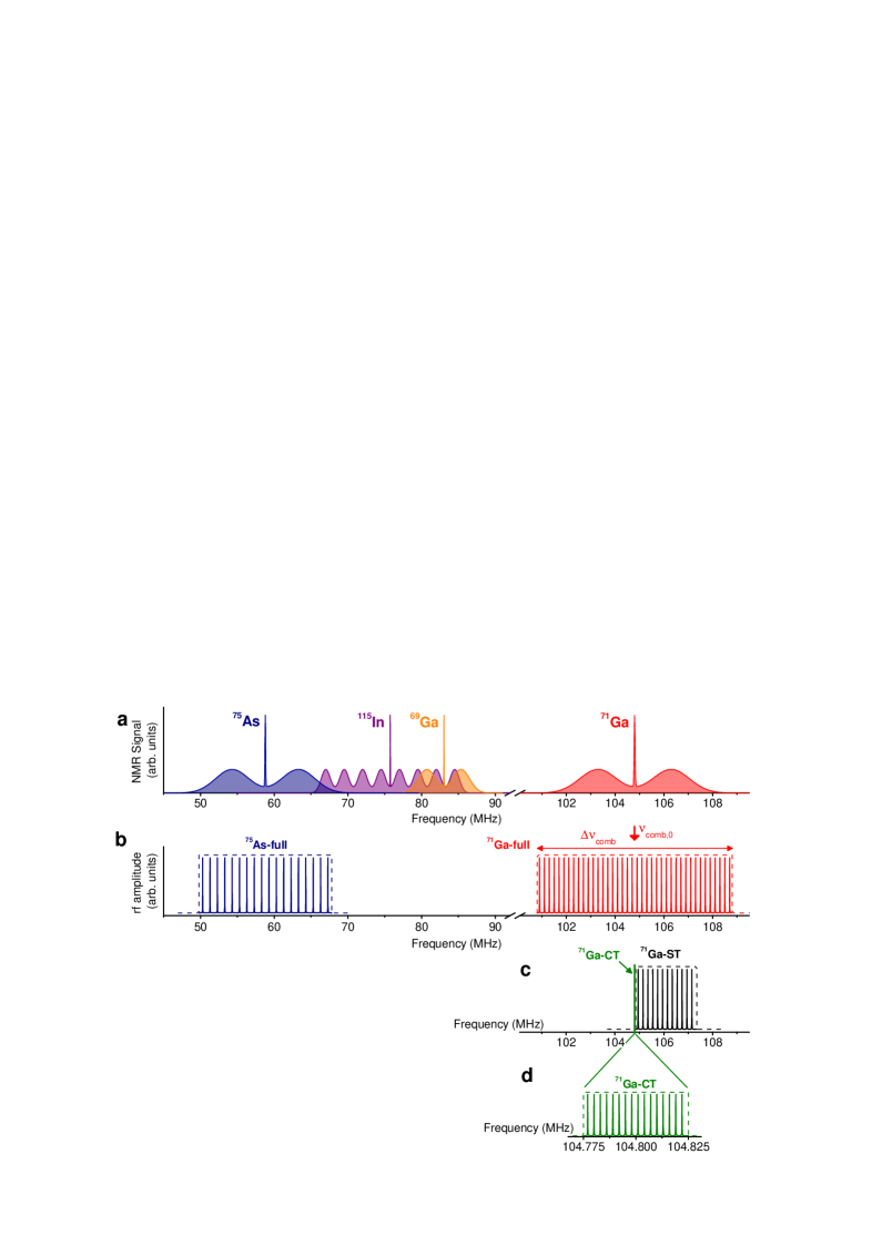
Supplementary Figure 1: Frequency combs for NMR experiments. a, Schematic NMR spectrum of a strained self-assembled InGaAs quantum dot at $B_{z}=8$ T. Sharp peaks arise from the central transitions (CTs) between $-1/2$ and $+1/2$ nuclear spin levels of each isotope. There are two satellite transitions (STs) for the spin-3/2 isotopes of Ga and As, and eight STs for the spin-9/2 indium. Inhomogeneous quadrupolar broadening results in significant overlap of the ¹¹⁵In and ⁶⁹Ga inhomogeneous lineshapes, while the overlap of ⁷⁵As and ¹¹⁵In is minimal. The ⁷¹Ga resonance is well isolated. b-d, Schematic spectra of the frequency combs used in experiments. The ⁷⁵As-full comb is used to excite the entire inhomogeneous lineshape of ⁷⁵As with minimum effect on ¹¹⁵In. Similarly ⁷¹Ga-full comb excites the entire ⁷¹Ga resonance. Frequency comb ⁷¹Ga-ST is used to excite selectively the $+1/2\leftrightarrow+3/2$ ST of ⁷¹Ga, while the comb ⁷¹Ga-CT is used to excite the $-1/2\leftrightarrow+1/2$ CT (zoom in is shown in d). The parameters of all frequency combs are summarized in Supplementary Table 1, further details can be found in Supplementary Note 1.1.

Supplementary Figure 2: Time diagram of an optically detected frequency-comb nuclear magnetic resonance experiment. See detailed explanation in Supplementary Note 1.2.

Supplementary Figure 3: Experimental verification of the rate equation model. a, Dynamics of the ⁷¹Ga nuclear spin depolarisation at $B_{z}=8$ T induced by frequency comb rf excitation with comb period $f_{\textrm{CP}}=31.25$ Hz. The results at high rf field density $\beta_{1}=86.0$ nT Hz^-1/2 (low rf field density $\beta_{1}=24.2$ nT Hz^-1/2) are shown by the squares (triangles). Solid lines show exponential fits with decay time $\tau\approx 23$ ms ($\tau\approx 290$ ms) for high (low) rf field density. b, c, Full $\Delta E_{\textrm{hf}}(t,f_{\textrm{CP}})$ dependence measured at high (b) and low rf (c) field densities.

Table Supplementary Table 1: Frequency comb parameters used in NMR experiments.

a, Homogeneous lineshape experiments (Fig. 2):
Isotope	75As	71Ga
Frequency comb	75As-full	71Ga-full
Comb central frequency $\nu_{\textrm{comb,0}}$ (MHz)	58.81	104.80
Comb spectral width $\Delta\nu_{\textrm{comb}}$ (MHz)	18	9
Comb period $f_{\textrm{CP}}$ (Hz)	varied	varied
Rf field density $\beta_{1}$ ($\textrm{nT}\ \textrm{Hz}^{-1/2}$)	65.5	39.1
b, Lineshape broadening experiments (Figs. 4a, 4b):
Isotope	75As	71Ga
Frequency comb	75As-full	71Ga-full
Comb central frequency $\nu_{\textrm{comb,0}}$ (MHz)	58.81	104.80
Comb spectral width $\Delta\nu_{\textrm{comb}}$ (MHz)	18	8
Comb period $f_{\textrm{CP}}$ (Hz)	varied	159
Rf field density $\beta_{1}$ ($\textrm{nT}\ \textrm{Hz}^{-1/2}$)	30.5	27.6
c, Correlation time experiments (Fig. 4c):
Isotope	75As	71Ga	71Ga	71Ga
Frequency comb	75As-full	71Ga-full	71Ga-ST	71Ga-CT
Comb central frequency $\nu_{\textrm{comb,0}}$ (MHz)	58.81	104.80	106.10	104.80
Comb spectral width $\Delta\nu_{\textrm{comb}}$ (MHz)	18	8	2.5	0.05
Comb period $f_{\textrm{CP}}$ (Hz)	1466	159	150	150
Rf field density $\beta_{1}$ ($\textrm{nT}\ \textrm{Hz}^{-1/2}$)	30.5	27.6	varied	varied

Supplementary Note 1 Details of experimental techniques

Supplementary Note 1.1 Frequency combs

The key novel findings of this work are based on the use of radiofrequency (rf) excitation with a frequency comb spectral profile. Here we give detailed parameters of the frequency combs used in the experiments on self-assembled quantum dots.

Supplementary Figure 1a shows a schematic NMR spectrum of a self-assembled InGaAs quantum dot at $B_{z}=8$ T, based on results of the inverse NMR measurements ¹. Four sharp peaks arise from the central transitions (CTs) $-1/2\leftrightarrow+1/2$ of each isotope. All spin-3/2 nuclei (⁷⁵As, ⁶⁹Ga and ⁷¹Ga) have two satellite transitions (STs) $-3/2\leftrightarrow-1/2$ and $+1/2\leftrightarrow+3/2$ observed as inhomogeneously broadened bands on both sides of the CTs. The spin-9/2 ¹¹⁵In nuclei have a total of eight STs. For clarity these are shown as four bands on each side of the CT, although in experimental NMR spectra the peaks arising from different STs merge forming two inhomogeneously broadened bands on both sides of the ¹¹⁵In CT ¹. As shown in Supplementary Figure 1a the spectral contributions from the ¹¹⁵In and ⁶⁹Ga nuclei overlap significantly; furthermore, there is a small overlap between the ⁷⁵As and ¹¹⁵In NMR resonances.

In the experiments we use rf frequency combs that are designed to influence only the chosen transition(s) of one isotope without affecting the other isotopes as demonstrated in Supplementary Figures 1b-d. The frequency-comb labeled ⁷¹Ga-full has a total width $\Delta\nu_{\textrm{comb}}$ of 8 or 9 MHz. This comb entirely covers the inhomogeneous lineshape of ⁷¹Ga and thus uniformly excites all nuclear spin transitions of this isotope. Since ⁷¹Ga has a large resonance frequency the ⁷¹Ga-full comb does not affect the polarisation of the other isotopes. To achieve selective excitation of the ⁷¹Ga ST ($+1/2\leftrightarrow+3/2$) we use frequency comb ⁷¹Ga-ST with $\Delta\nu_{\textrm{comb}}=2.5$ MHz (Supplementary Fig. 1c). Similarly, selective excitation of ⁷¹Ga CT is achieved with a narrow comb ⁷¹Ga-CT with a width of $\Delta\nu_{\textrm{comb}}=50$ kHz as shown in Supplementary Figs. 1c, d.

In the case of ⁷⁵As we use a frequency comb ⁷⁵As-full that excites the entire inhomogeneouse resonance line. This comb inevitably excites some of the ¹¹⁵In nuclear transitions, mostly $-9/2\leftrightarrow-7/2$ STs. However, excitation of the $-9/2\leftrightarrow-7/2$ ST alone has a negligible effect on the overall change in the nuclear polarisation of the spin-9/2 nuclei of ¹¹⁵In. Thus the ⁷⁵As-full comb with the optimum width $\Delta\nu_{\textrm{comb}}=18$ MHz is used in experiments for selective depolarisation of ⁷⁵As.

The central frequencies $\nu_{\textrm{comb,0}}$, the widths $\Delta\nu_{\textrm{comb}}$ and the comb periods (spectral separation between the adjacent modes) $f_{\textrm{CP}}$ of all the combs used in experiments are listed in Supplementary Table 1. Depending on the experiment the $f_{\textrm{CP}}$ is either varied or kept constant. Typically the values of $f_{\textrm{CP}}$ ranging from 30 Hz to 21 kHz are employed, so that the total number of modes in the comb $N_{\textrm{m}}=\Delta\nu_{\textrm{comb}}/f_{\textrm{CP}}+1$ ranges from $\sim$330 to $\sim$600000.

The phases of individual modes of the frequency comb are chosen in a way that minimizes the peak power for a given average power (i.e. a waveform with the minimum crest-factor). In particular the following expression satisfies this criterion:

$$B_{\textrm{rf}}(t)=B_{1}\sum_{j=1}^{N_{\textrm{m}}}\cos\left(2\pi\left(\nu_{1}+(j-1)f_{\textrm{CP}}\right)t+\pi\frac{j(j-1)}{N_{\textrm{m}}}\right),$$ (1)

where the summation goes over all modes, and $\nu_{1}$ is the frequency of the first mode of the comb. In experiments the frequency-comb signal is generated by an arbitrary waveform generator equipped with a 64 million points memory.

Each mode of the frequency comb has the same amplitude $B_{1}$ of the rf oscillating magnetic field. In experiments where the comb period $f_{\textrm{CP}}$ is varied $B_{1}$ has to be adjusted to maintain the same total power of the frequency comb excitation. Since the power is proportional to $B_{1}^{2}$ the $B_{1}^{2}/f_{\textrm{CP}}$ ratio has to be kept constant. Thus the amplitude of the frequency comb can be conveniently characterized by the magnetic field density $\beta_{\textrm{1}}=B_{1}/\sqrt{f_{\textrm{CP}}}$.

The amplitude of the frequency comb rf magnetic field can be calibrated from an additional pulsed Rabi oscillation experiment on the CT of a selected isotope ². The Rabi oscillation circular frequency $\omega_{\textrm{Rabi}}$ can be measured experimentally and is proportional to the rf field amplitude $B_{\textrm{rf}}$ in the rotating frame:

$$B_{\textrm{rf}}=\frac{\omega_{\textrm{Rabi}}}{2\gamma},$$ (2)

where $\gamma$ is nuclear gyromagnetic ratio and the factor $2$ originates from the dipole transition matrix element of the CT of a spin-3/2 nucleus ³. Throughout all experiments, we monitored the applied rf fields via a pick-up coil that was placed close to the sample and connected to a spectrum analyzer. By comparing the voltages induced by the frequency comb modes with the voltage associated with a field $B_{\textrm{rf}}$ in the Rabi oscillation experiment, we derived the values of $B_{1}$ and $\beta_{\textrm{1}}$ of the comb. The values of $\beta_{\textrm{1}}$ used in different experiments are given in Supplementary Table 1 - these correspond to the rotating frame, i.e. the physical values of the magnetic field induced by the coil are twice as large.

Supplementary Note 1.2 Optical pump-probe techniques for frequency-comb NMR

Supplementary Fig. 2 shows the time sequence of optical and rf excitation pulses used in a frequency comb measurement of the equilibrium nuclear spin bath fluctuations of the ⁷¹Ga isotope (the results are shown in Fig. 4c of the main text). As explained in the main text this experiment is based on measuring the rf induced dynamics of the ⁷⁵As spins in the presence of additional rf excitation of ⁷¹Ga spins. The experimental cycle consists of the following four stages described below.

Optical nuclear spin pumping. At the start of each new measurement cycle, the nuclear spin bath is reinitialized optically. This is achieved with optically induced dynamic nuclear polarisation (DNP) ^{4, 5}: under high power, circularly polarised laser excitation, spin polarised electrons are created. These electrons can efficiently transfer their polarisation to the nuclear spin bath via hyperfine interaction ⁶. We use $\sigma^{-}$ polarised excitation with a pump laser operating at $\sim$850 nm, in resonance with the QD wetting layer. By using sufficiently long pumping times ($t_{\textrm{Pump}}=5.5-6.5$ s) and high powers $\sim 10P_{\textrm{sat}}$ (where $P_{\textrm{sat}}$ is the saturation power of the QD ground states), we create a reproducible and high degree of nuclear polarisation.

Depolarisation of ⁷¹Ga isotope. Optical spin pumping polarises the nuclei of all isotopes. However, in order to probe the equilibrium fluctuations of ⁷¹Ga spins their longitudinal relaxation has to be excluded from the measured dynamics. For that ⁷¹Ga nuclear polarisation has to be erased, which is achieved by exciting the spins with a ⁷¹Ga-full frequency comb for a sufficiently long time $t_{\textrm{Depol}}=1.2$ s. To simplify experimental implementation the depolarising rf is kept on during the nuclear spin pumping stage as well, which has no effect on the experimental results.

Frequency comb rf excitation. Following the spin bath preparation (optical DNP and ⁷¹Ga depolarisation), the main rf excitation (variable duration $t_{\textrm{rf}}$) is applied. For the spin bath fluctuation measurement (Fig. 4c) this excitation is a sum of the ⁷⁵As-full frequency comb and either the ⁷¹Ga-ST or the ⁷¹Ga-CT comb. Since ⁷¹Ga is completely depolarised by the previous pulse, all changes in the total nuclear polarisation at this stage are solely due to the ⁷⁵As depolarisation. In this way we ensure that it is the depolarisation dynamics of ⁷⁵As that is measured, while the ⁷¹Ga-ST or ⁷¹Ga-CT ”heating” excitation only induces nuclear spin-flips of the corresponding ⁷¹Ga transition.

Optical probing of the nuclear spin polarisation. At the end of the experiment cycle, a short probe laser pulse is applied and the resulting photoluminescence spectrum is collected by a 1 m double spectrometer with a CCD. The changes in the quantum dot Zeeman splitting (the Overhauser shift $E_{\textrm{hf}}$) are used to probe the nuclear spin state. The probe laser is non-resonant ($\sim 850$ nm), yet unlike the pump laser it is linearly polarised and the probe power and duration $t_{\textrm{Probe}}$ are chosen such that no noticeable DNP is induced and the final nuclear spin polarisation is measured accurately. Typical probe parameters used in the experiments were $t_{\textrm{Probe}}=4$ ms and $\sim P_{\textrm{sat}}/10$ for QDs in the $p-i-n$ diode sample and $t_{\textrm{Probe}}=60$ ms and $\sim P_{\textrm{sat}}/50$ in the gate-free structure. Depending on the QD photoluminescence intensity the experiment cycle was repeated $10-40$ times to achieve the optimum signal-to-noise ratio.

For the purpose of data analysis we are interested in measuring the rf-induced change in the nuclear spin polarisation (rf-induced change in the Overhauser shift $\Delta E_{\textrm{hf}}$), for that we perform a control measurement where ⁷⁵As-full comb is off, and subtract the resulting QD Zeeman splitting from the Zeeman splittings obtained in the measurements with ⁷⁵As excitation. In this way $\Delta E_{\textrm{hf}}=0$ corresponds to no nuclear spin depolarisation induced by the rf.

The diagram of Supplementary Fig. 2 also describes the other types of frequency comb NMR measurements presented in the main text with the following modifications: For the line broadening measurements shown in Figs. 4a, b the main excitation is a sum of the ⁷⁵As-full and ⁷¹Ga-full frequency combs (the ⁷¹Ga-full is off for the measurement in Fig. 4a and is on for Fig. 4b). The homogeneous lineshape measurement (Fig. 2) is performed without the additional rf depolarisation excitation, while for the main rf excitation the ⁷¹Ga-full comb is used.

Supplementary Note 2 Theoretical model for nuclear spin dynamics under frequency-comb excitation

The Methods section of the main text describes the model for spin $I=1/2$ nuclei. Here we consider a more general case of nuclear spins $I>1/2$ with gyromagnetic ratio $\gamma$. We consider the Overhauser shifts of nuclei of only one isotope, which is justified since the polarisation of other isotopes stays constant during the measurement and can be neglected. In an external magnetic field the nuclear spin state is split into $2I+1$ states with spin projections $I_{\textrm{z}}=-I,\ -I+1,\ ...\ I-1,\ +I$. In our classical rate equation model we assume that each nuclear spin has a probability $p_{\textrm{m}}$ to be found in a state with $I_{\textrm{z}}=m$ with normalization condition

$$\sum_{m=-I}^{I}p_{m}(t)=1.$$ (3)

We also assume that at $t=0$ optical pumping initializes all nuclear spins into a Boltzman distribution

$$p_{m}(t=0)=p_{m,0}\propto\exp(\xi m),$$ (4)

so that nuclear spins can be characterized by a temperature $T_{\textrm{nuc}}\propto 1/\xi$. When optical nuclear spin pumping is used, $T_{\textrm{nuc}}$ is very small compared to the spin bath temperature $T$, so the equilibrium nuclear polarisation can be neglected.

Application of the radiofrequency (rf) excitation leads to the changes in population probabilities. The rf excites only dipole-allowed transitions for which $I_{\textrm{z}}$ changes by $\pm 1$. In the experiment we use weak, non-saturating radiofrequency fields. Thus instead of the full Bloch equations for nuclear magnetization, the evolution of the population probabilities of the states with $I_{\textrm{z}}=m$ can be described with the following first-order differential equation (see further details in Supplementary Note 3):

$$\begin{aligned} &dp_{m}/dt=-(W_{m-1,m}+W_{m,m+1})p_{m}(t)+W_{m-1,m}p_{m-1}(t)+W_{m,m+1}p_{m+1}(t),\ -I<m<I\\ &dp_{I}/dt=W_{I-1,I}(-p_{I}(t)+p_{I-1}(t))\\ &dp_{-I}/dt=W_{-I,-I+1}(-p_{-I}(t)+p_{-I+1}(t)).\end{aligned}$$ (5)

Here the first equation describes the states with $-I<I_{z}<I$. Its first term is due to nuclei with $I_{\textrm{z}}=m$ making transitions into the $I_{\textrm{z}}=m-1$ and $m+1$ states, whereas the second and third terms describe the opposite case of nuclei transitioning into the $I_{\textrm{z}}=m$ state from the $I_{\textrm{z}}=m-1$ and $I_{\textrm{z}}=m+1$ states respectively. The second and third equations correspond to the case of $m=-I$ and $m=+I$ respectively. Taken for all $m$, for which $-I\leq m\leq I$, the Supplementary Eq. 5 yields a system of $2I+1$ first-order ordinary differential equations (ODEs) for $2I+1$ time-dependent variables $p_{m}(t)$ with initial conditions given by Supplementary Eq. 4. Due to the normalization condition of Supplementary Eq. 3, only $2I$ variables and equations are independent. This system of ODEs has a tridiagonal matrix with coefficients determined by the rf induced transition rates $W_{m,m+1}$ which satisfy a symmetry condition $W_{m,m+1}=W_{m+1,m}$.

Similar to the case of $I=1/2$, each transition rate $W_{m,m+1}$ resulting from the frequency-comb excitation is a sum of transition rates caused by individual rf modes each having magnetic field amplitude $B_{\textrm{1}}$. We assume that each nuclear transition has the same broadening described by the homogeneous lineshape function $L(\nu)$, with normalization $\int_{-\infty}^{+\infty}L(\nu)d\nu=1$. Due to the inhomogeneous quadrupolar shifts the NMR transition frequency $\nu_{\textrm{m,m+1}}$ is generally different for each pair of spin levels $I_{\textrm{z}}=m$ and $I_{\textrm{z}}=m+1$ (even for one nucleus). Thus for the transition rates we can write:

$$W_{m,m+1}(\nu_{m,m+1})=\frac{(I-m)(I+m+1)\gamma^{2}B_{\textrm{1}}^{2}}{2f_{\textrm{CP}}}\sum_{j=-\infty}^{+\infty}L(\nu_{m,m+1}-\nu_{1}-jf_{\textrm{CP}})f_{\textrm{CP}},$$ (6)

where the summation goes over all modes with frequencies $\nu_{\textrm{j}}=\nu_{\textrm{1}}+(j-1)f_{\textrm{CP}}$, and is extended to $\pm\infty$ since the total width of the rf excitation comb $\Delta\nu_{\textrm{comb}}$ is much larger than $f_{\textrm{CP}}$ and the homogeneous linewidth $\Delta\nu_{\textrm{hom}}$. The $(I-m)(I+m+1)$ factor arises from the dipolar transition matrix element ³. We note that Supplementary Eq. 5 does not involve any explicit nuclear-nuclear interactions. Instead such interactions are introduced in Supplementary Eq. 6 phenomenologically via the homogeneous broadening described by the lineshape function $L(\nu)$. On the other hand the presence of finite homogeneous broadening is essential in order to use the limit of weak rf fields ⁷ and transform the Bloch equations into rate equations (Supplementary Eq. 5). The validity of the weak rf field approximation is discussed and verified experimentally in Supplementary Note 3.

Since Supplementary Eq. 5 is a system of linear first-order equations, the solution is a multiexponential relaxation towards the fully depolarised state where all nuclear spin states have equal populations $p_{m}=1/(2I+1)$. The solution has the general form:

$$p_{m}(t)=1/(2I+1)+\sum_{\textrm{j=1}}^{2I}a_{m,\textrm{j}}\exp(-\lambda_{\textrm{j}}t),$$ (7)

where $\lambda_{\textrm{j}}$ are the non-zero eigenvalues of the ODE system matrix of Supplementary Eq. 5. The values of $\lambda_{\textrm{j}}$ depend on all transition rates $W_{m,m+1}$ from Supplementary Eq. 6, while the coefficients $a_{m,\textrm{j}}$ depend both on $W_{m,m+1}$ and the initial probabilities $p_{m,0}$ from Supplementary Eq. 4.

Non-zero nuclear spin polarisation along the magnetic field ($Oz$ axis) changes the spectral splitting of the quantum dot Zeeman doublet. Such change known as the Overhauser shift is measured experimentally using photoluminescence spectroscopy. The time evolution of the Overhauser shift for the fixed values of nuclear transition frequencies $\{\nu_{m,m+1}\}=\{\nu_{-I,-I+1},\ \nu_{-I+1,-I+2},\ ...\ \nu_{I-1,I}\}$ reads as:

$$E_{\textrm{hf,1}}(t,f_{\textrm{CP}},B_{1},T_{\textrm{nuc}},L(\nu),\{\nu_{m,m+1}\})=A\sum_{m=-I}^{+I}mp_{m}(t),$$ (8)

where $A$ is the hyperfine constant and we used Supplementary Eqns. 4, 6, 7 so that $E_{\textrm{hf,1}}$ is dependent on $f_{\textrm{CP}}$, $B_{\textrm{1}}$, $T_{\textrm{nuc}}$, the homogeneous lineshape function $L(\nu)$ and all nuclear transition frequencies $\{\nu_{m,m+1}\}$ as parameters.

Each QD contains a large number of nuclear spins with randomly distributed absorption frequencies. Thus to describe the experiment on nuclear spins in a self-assembled quantum dot we need to average over all $\nu_{\textrm{m,m+1}}$, which can be done over one period $f_{\textrm{CP}}$ since the spectrum of the frequency-comb rf excitation is periodic. Similarly to the case of $I=1/2$, the following expression is obtained for the time dependence of the Overhauser shift, describing the dynamics of rf-induced nuclear spin depolarisation:

$$\begin{aligned} &E_{\textrm{hf}}(t,f_{\textrm{CP}},B_{1},T_{\textrm{nuc}},L(\nu))=\\ &f_{\textrm{CP}}^{-2I}\int\limits_{0}^{f_{\textrm{CP}}}d\nu_{-I,-I+1}\ ...\int\limits_{0}^{f_{\textrm{CP}}}d\nu_{I-1,I}\ E_{\textrm{hf,1}}(t,f_{\textrm{CP}},B_{1},T_{\textrm{nuc}},L(\nu),\{\nu_{m,m+1}\}).\end{aligned}$$ (9)

The quantity measured in the experiment is the rf-induced variation of the Overhauser shift:

$$\begin{aligned} \Delta E_{\textrm{hf}}(t,f_{\textrm{CP}},B_{1},T_{\textrm{nuc}},L(\nu))=E_{\textrm{hf}}(t,f_{\textrm{CP}},B_{1},T_{\textrm{nuc}},L(\nu))-E_{\textrm{hf}}(t=0).\end{aligned}$$ (10)

The values of $f_{\textrm{CP}}$ and $B_{\textrm{1}}$ are the parameters that are controlled in the experiment. The nuclear spin temperature $T_{\textrm{nuc}}$ can be determined using the known hyperfine constant $A$ and the measured total Overhauser shift $\Delta E_{\textrm{hf}}(t=\infty)$. Thus for a given homogeneous NMR lineshape $L(\nu)$ the nuclear spin depolarisation dynamics can be fully predicted from Supplementary Eqns. 3–10. Conversely, Supplementary Eq. 9 can be treated as an integral equation on the unknown homogeneous lineshape function $L(\nu)$. Since Fredholm’s integral equation of the first kind is an ill-conditioned problem, some constrains on $L(\nu)$ are required. Our approach is to use a model lineshape with two parameters $\Delta\nu_{\textrm{hom}}$ and $k$ (Eq. 1 of the main text). Upon substituting this model lineshape the Overhauser shift variation of Supplementary Eq. 10 becomes $\Delta E_{\textrm{hf}}(t,f_{\textrm{CP}},B_{1},T_{\textrm{nuc}},\Delta\nu_{\textrm{hom}},k)$. We then perform least-square fitting to the experimental dependence $\Delta E_{\textrm{hf}}(t,f_{\textrm{CP}})$ using $B_{1}$, the homogeneous linewidth $\Delta\nu_{\textrm{hom}}$ and the roll-off parameter $k$ as fitting parameters and using the nuclear spin temperature $T_{\textrm{nuc}}$ obtained from the experiment.

The ODE system of Supplementary Eq. 5 can be solved analytically for $I\leq 3/2$, however it turns out to be more practical to perform numerical diagonalization in order to obtain the eigenvalues $\lambda_{\textrm{j}}$ and coefficients $a_{m,\textrm{j}}$ which are then used in Supplementary Eq. 7. Similarly we use numerical integration to evaluate Supplementary Eq. 9.

Supplementary Note 3 Applicability of the frequency comb technique and the rate equation model.

The evolution of the nuclear magnetization under rf excitation can be described by the Bloch equations ⁸. In this model the solution under resonant monochromatic excitation is determined by the three important parameters: the amplitude of the resonant field $B_{\textrm{rf}}$, and the relaxation times characterizing the system, the longitudinal $T_{1}$ and the transverse $T_{2}$. In self-assembled quantum dots $T_{1}$ is extremely long (few hours ^{9, 10}), so that the longitudinal relaxation can be neglected. Thus the nuclear spin dynamics is determined by the relation between $B_{\textrm{rf}}$ and $T_{2}$. Two cases are possible ⁷. If rf magnetic field is strong ($\gamma B_{\textrm{rf}}T_{2}\gg 1$) the nuclear magnetization has oscillatory behaviour (Rabi oscillations are observed). By contrast, for weak rf excitation ($\gamma B_{\textrm{rf}}T_{2}\ll 1$) there are no oscillations, and any nuclear magnetization $I_{z}$ along the external field decays exponentially to its steady state value ⁷. The exponential dynamics in the weak rf excitation regime allow for the problem to be simplified and for the rate equation model described by Supplementary Eqns. 5 to be used. The validity of the rate equation model is essential for the determination of the homogeneous lineshape and thus sets the applicability limit for the frequency comb technique itself.

To verify the applicability of the rate equation model we performed frequency comb spectroscopy measurements at different rf amplitudes. Supplementary figure 3 shows the results for ⁷¹Ga measured at high rf field density $\beta_{1}=86.0$ nT Hz^-1/2 and low rf field density $\beta_{1}=24.2$ nT Hz^-1/2 – in all other respects the conditions in these experiments were the same as in the experiment with medium $\beta_{1}=39.1$ nT Hz^-1/2 shown in Fig. 2 of the main text.

The Supplementary figure 3a shows by symbols the nuclear spin depolarisation dynamics at small comb period $f_{\textrm{CP}}=31.25$ Hz. At low rf field amplitude $\beta_{1}=24.2$ nT Hz^-1/2 (triangles) the decay can be described very well by a single exponential decay ($\tau\approx 290$ ms) shown with a solid line. By contrast, at high amplitude $\beta_{1}=86.0$ nT Hz^-1/2 (squares) the dynamics shows signatures of oscillations, and there is a clear deviation from the exponential behaviour (best exponential fit is for $\tau\approx 23$ ms).

Supplementary Figures 3b and c show the full $\Delta E_{\textrm{hf}}(t,f_{\textrm{CP}})$ dependencies measured at high (b) and low rf (c) field densities. The $\Delta E_{\textrm{hf}}(t,f_{\textrm{CP}})$ profiles are in good agreement for the two experiments (except for the rescaling along the $t_{\textrm{rf}}$ axis). Using model fitting we find $\Delta\nu_{\textrm{hom}}\approx 244$ Hz, $k\approx 1.66$ for $\beta_{1}=86.0$ nT Hz^-1/2 and $\Delta\nu_{\textrm{hom}}\approx 223$ Hz, $k\approx 1.68$ for $\beta_{1}=24.2$ nT Hz^-1/2. This is also in good agreement with $\Delta\nu_{\textrm{hom}}\approx 221$ Hz, $k\approx 1.67$ found for the measurement at $\beta_{1}=39.1$ nT Hz^-1/2 shown in Fig. 2 of the main text.

We thus conclude that the discrepancy between the results in Supplementary Figs. 3b and c becomes significant only at small comb period $f_{\textrm{CP}}=31.25$ Hz (as also demonstrated in Supplementary Figure 3a). This can be explained as follows: At high rf excitation amplitude the nuclear spin depolarisation takes place on a shorter time scale $\tau$. If the rf pulses are shorter than $1/f_{\textrm{CP}}$, the spectral profile of the frequency comb becomes distorted. Thus if the nuclear polarisation decay timescales $\tau$ are shorter than $1/f_{\textrm{CP}}$, the rate equation model is no longer applicable since the rf excitation can not be described as a frequency comb. Thus it is required that $\tau>1/f_{\textrm{CP}}$. Furthermore, to measure the homogeneous lineshape and linewidth $\Delta\nu_{\textrm{hom}}$ we only need to use frequency combs with comb periods $f_{\textrm{CP}}$ comparable to or larger than $\Delta\nu_{\textrm{hom}}$, so it is required that $f_{\textrm{CP}}\in\{\Delta\nu_{\textrm{hom}},\infty\}$. Combining $\tau>1/f_{\textrm{CP}}$ and $f_{\textrm{CP}}\in\{\Delta\nu_{\textrm{hom}},\infty\}$ we find the following condition on the frequency comb technique applicability:

$$\begin{aligned} \Delta\nu_{\textrm{hom}}>1/\tau,\end{aligned}$$ (11)

which restricts the rf amplitude, characterized by the depolarisation time $\tau$.

Another requirement, arising from the applicability of the weak rf field limit of the Bloch equations, is that the rf induced depolarisation time $\tau$ must be longer than the transverse relaxation time $T_{2}$. However, $T_{2}$ is related to the homogeneous linewidth as $T_{2}\sim 1/(\pi\Delta\nu_{\textrm{hom}})$. Thus the requirement $\tau>T_{2}$ leads to the same condition as that of Supplementary Eq. 11. Furthermore, since the frequency comb technique relies on the measurement of the longitudinal nuclear magnetization, the depolarisation time $\tau$ must be shorter than the nuclear spin $T_{1}$ times. In combination with Supplementary Eq. 11 this leads to the following condition:

$$\begin{aligned} \Delta\nu_{\textrm{hom}}>1/\tau>1/T_{1}\end{aligned}$$ (12)

This condition has a dual role: it sets the boundaries for the rf excitation amplitude (characterized by $\tau$) and sets the limitation $\Delta\nu_{\textrm{hom}}>1/T_{1}$ on the properties of the nuclear spin system that can be studied with the frequency comb technique. This latter condition can be rewritten as

$$\begin{aligned} T_{1}>aT_{2}\end{aligned}$$ (13)

From the measurements at different rf amplitudes we find that the parameter $a$ must be $a\sim 10-100$ or larger in order for the frequency comb technique to work reliably. This however is a rather weak condition and is satisfied for a large class of solid-state nuclear spin systems where $T_{1}\gg T_{2}$. This demonstrates the wide applicability of the frequency comb spectroscopy technique developed here.

References

- 1 Borri, P., Langbein, W., Schneider, S., Woggon, U., Sellin, R. L., Ouyang, D., and Bimberg, D. Ultralong dephasing time in InGaAs quantum dots. Phys. Rev. Lett. 87, 157401 (2001).
- 2 Volker, S. Hole-burning spectroscopy. Annual Review of Physical Chemistry 40, 499–530 (1989).
- 3 Yang, L., Glasenapp, P., Greilich, A., Reuter, D., Wieck, A. D., Yakovlev, D. R., Bayer, M., and Crooker, S. A. Two-colour spin noise spectroscopy and fluctuation correlations reveal homogeneous linewidths within quantum-dot ensembles. Nature Communications 5, 5949 (2014).
- 4 Hahn, E. L. Spin echoes. Physical Review 80, 580 (1950).
- 5 Biercuk, M. J., Uys, H., VanDevender, A. P., Shiga, N., Itano, W. M., and Bollinger, J. J. Optimized dynamical decoupling in a model quantum memory. Nature 458, 996–1000 (2009).
- 6 Bar-Gill, N., Pham, L., Belthangady, C., Le Sage, D., Cappellaro, P., Maze, J., Lukin, M., Yacoby, A., and Walsworth, R. Suppression of spin-bath dynamics for improved coherence of multi-spin-qubit. Nature Communications 3, 858 (2012).
- 7 Tyryshkin, A. M., Tojo, S., Morton, J. J. L., Riemann, H., Abrosimov, N. V., Becker, P., Pohl, H.-J., Schenkel, T., Thewalt, M. L. W., Itoh, K. M., and Lyon, S. A. Electron spin coherence exceeding seconds in high-purity silicon. Nature Mater. 11, 143–147 (2012).
- 8 Li, D., Dementyev, A. E., Dong, Y., Ramos, R. G., and Barrett, S. E. Generating unexpected spin echoes in dipolar solids with pulses. Phys. Rev. Lett. 98, 190401 (2007).
- 9 Merkulov, I. A., Efros, A. L., and Rosen, M., Electron spin relaxation by nuclei in semiconductor quantum dots. Phys. Rev. B 65, 205309 (2002).
- 10 de Sousa, R. and Das Sarma, S., Theory of nuclear-induced spectral diffusion: Spin decoherence of phosphorus donors in and quantum dots. Phys. Rev. B 68, 115322 (2003).
- 11 Yao, W., Liu, R.-B., and Sham, L. J., Theory of electron spin decoherence by interacting nuclear spins in a quantum dot. Phys. Rev. B 74, 195301 (2006).
- 12 Bluhm, H., Foletti, S., Neder, I., Rudner, M., Mahalu, D., Umansky, V., and Yacoby, A., Dephasing time of electron-spin qubits coupled to a nuclear bath exceeding 200 s. Nature Physics 7, 109 (2011).
- 13 Press, D., De Greve, K., McMahon, P. L., Ladd, T. D., Friess, B., Schneider, C., Kamp, M., Hofling, S., Forchel, A., and Yamamoto, Y. Ultrafast optical spin echo in a single quantum dot. Nature Photon. 4, 367–370 (2010).
- 14 De Greve, K., McMahon, P. L., Press, D., Ladd, T. D., Bisping, D., Schneider, C., Kamp, M., Worschech, L., Hofling, S., Forchel, A., and Yamamoto, Y., Ultrafast coherent control and suppressed nuclear feedback of a single quantum dot hole qubit. Nature Phys. 7, 872 (2011).
- 15 Greilich, A., Carter, S. G., Kim, D., Bracker, A. S., and Gammon, D., Optical control of one and two hole spins in interacting quantum dots. Nature Photon. 5, 702–708 (2011).
- 16 Hansom, J., Schulte, C. H. H., Le Gall, C., Matthiesen, C., Clarke, E., Hugues, M., Taylor, J. M., and Atature, M. Environment-assisted quantum control of a solid-state spin via coherent dark states. Nature Phys. 10, 1745–2473 (2014).
- 17 Urbaszek, B., Marie, X., Amand, T., Krebs, O., Voisin, P., Maletinsky, P., Högele, A., and Imamoglu, A., Nuclear spin physics in quantum dots: An optical investigation. Rev. Mod. Phys. 85, 79–133 (2013).
- 18 Cai, J., Retzker, A., Jelezko, F., and Plenio, M. B. A large-scale quantum simulator on a diamond surface at room temperature. Nature Physics 9, 168–173 (2013).
- 19 de Sousa, R. and Das Sarma, S. Electron spin coherence in semiconductors: Considerations for a spin-based solid-state quantum computer architecture. Phys. Rev. B 67, 033301, Jan (2003).
- 20 Chekhovich, E., Hopkinson, M., Skolnick, M., and Tartakovskii, A. Suppression of nuclear spin bath fluctuations in self-assembled quantum dots induced by inhomogeneous strain. Nature Communications 6, 7348 (2015).
- 21 Chekhovich, E. A., Kavokin, K. V., Puebla, J., Krysa, A. B., Hopkinson, M., Andreev, A. D., Sanchez, A. M., Beanland, R., Skolnick, M. S., and Tartakovskii, A. I. Structural analysis of strained quantum dots using nuclear magnetic resonance. Nature Nanotech. 7, 646–650 (2012).
- 22 Munsch, M., Wust, G., Kuhlmann, A. V., Xue, F., Ludwig, A., Reuter, D., Wieck, A. D., Poggio, M., and Warburton, R. J. Manipulation of the nuclear spin ensemble in a quantum dot with chirped magnetic resonance pulses. Nature Nanotechnology 9, 671–675 (2014).
- 23 Udem, T., Holzwarth, R., and Hansch, T. W. Optical frequency metrology. Nature 416, 233–237 (2002).
- 24 Dzhioev, R. I. and Korenev, V. L., Stabilization of the electron-nuclear spin orientation in quantum dots by the nuclear quadrupole interaction. Phys. Rev. Lett. 99, 037401 (2007).
- 25 Latta, C., Srivastava, A. and Imamoglu, A., Hyperfine interaction-dominated dynamics of nuclear spins in self-assembled InGaAs quantum dots. Phys. Rev. Lett. 107, 167401 (2011).
- 26 Van Vleck, J. H. The dipolar broadening of magnetic resonance lines in crystals. Phys. Rev. 74, 1168–1183 (1948).
- 27 Khaetskii, A. V., Loss, D., and Glazman, L., Electron spin decoherence in quantum dots due to interaction with nuclei. Phys. Rev. Lett. 88, 186802 (2002).
- 28 Muhonen, J. T., Dehollain, J. P., Laucht, A., Hudson, F. E., Kalra, R., Sekiguchi, T., Itoh, K. M., Jamieson, D. N., McCallum, J. C., Dzurak, A. S., and Morello, A. Storing quantum information for 30 seconds in a nanoelectronic device. Nature Nanotechnology 9, 986–991 (2014).
- 29 Neumann, P., Kolesov, R., Naydenov, B., Beck, J., Rempp, F., Steiner, M., Jacques, V., Balasubramanian, G., Markham, M. L., Twitchen, D. J., Pezzagna, S., Meijer, J., Twamley, J., Jelezko, F., and Wrachtrup, J., Quantum register based on coupled electron spins in a room-temperature solid. Nature Phys. 6, 249–253 (2010).

References

- 1 Chekhovich, E. A., Kavokin, K. V., Puebla, J., Krysa, A. B., Hopkinson, M., Andreev, A. D., Sanchez, A. M., Beanland, R., Skolnick, M. S., and Tartakovskii, A. I., Structural analysis of strained quantum dots using nuclear magnetic resonance. Nature Nanotech. 7, 646–650 (2012).
- 2 Chekhovich, E., Hopkinson, M., Skolnick, M., and Tartakovskii, A. Suppression of nuclear spin bath fluctuations in self-assembled quantum dots induced by inhomogeneous strain. Nature Communications 6, 7348 (2015).
- 3 Abragam, A., The principles of Nuclear Magnetism. Oxford University Press, London (1961).
- 4 Eble, B., Krebs, O., Lemaitre, A., Kowalik, K., Kudelski, A., Voisin, P., Urbaszek, B., Marie, X., and Amand, T., Dynamic nuclear polarization of a single charge-tunable quantum dot. Phys. Rev. B 74, 081306 (2006).
- 5 Puebla, J., Chekhovich, E. A., Hopkinson, M., Senellart, P., Lemaitre, A., Skolnick, M. S., and Tartakovskii, A. I., Dynamic nuclear polarization in and quantum dots under nonresonant ultralow-power optical excitation. Phys. Rev. B 88, 045306 (2013).
- 6 Gammon, D., Efros, A. L., Kennedy, T. A., Rosen, M., Katzer, D. S., Park, D., Brown, S. W., Korenev, V. L., and Merkulov, I. A. Electron and nuclear spin interactions in the optical spectra of single quantum dots. Phys. Rev. Lett. 86(22), 5176–5179 (2001).
- 7 Madhu, P. and Kumar, A. Direct cartesian-space solutions of generalized bloch equations in the rotating frame. Journal of Magnetic Resonance, Series A 114, 201 – 211 (1995).
- 8 Bloch, F. Nuclear induction. Physical Review 70, 460 (1946).
- 9 Latta, C., Srivastava, A., and Imamoğlu, A. Hyperfine interaction-dominated dynamics of nuclear spins in self-assembled quantum dots. Phys. Rev. Lett. 107, 167401 (2011).
- 10 Chekhovich, E. A., Makhonin, M. N., Skiba-Szymanska, J., Krysa, A. B., Kulakovskii, V. D., Skolnick, M. S., and Tartakovskii, A. I. Dynamics of optically induced nuclear spin polarization in individual quantum dots. Phys. Rev. B 81, 245308 (2010).