Stability results for sections
of convex bodies

Abstract.

It is shown by Makai, Martini, and Ódor that a convex body $K$, all of whose maximal sections pass through the origin, must be origin-symmetric. We prove a stability version of this result. We also discuss a theorem of Koldobsky and Shane about determination of convex bodies by fractional derivatives of the parallel section function and establish the corresponding stability result.

1. Introduction

Let $K$ be a convex body in $\mathbb{R}^{n}$, i.e. a compact convex set with non-empty interior. More generally, a body is a compact subset of $\mathbb{R}^{n}$ which is equal to the closure of its interior. Throughout the paper, we assume all bodies include the origin as an interior point. Now, we say $K$ is origin-symmetric if $K=-K$. The parallel section function of $K$ in the direction $\xi\in S^{n-1}$ is defined by

$$A_{K,\xi}(t)=\mathrm{vol}_{n-1}(K\cap\{\xi^{\perp}+t\xi\}),\quad t\in\mathbb{R}.$$

Here, $\xi^{\perp}=\{x\in\mathbb{R}^{n}:\,\langle x,\xi\rangle=0\}$ is the hyperplane passing through the origin and orthogonal to the vector $\xi$.

For the study of central sections it is often more natural to consider a larger class of bodies than the class of convex bodies. Recall that if $K$ is a body containing the origin in its interior and star-shaped with respect to the origin, its radial function is defined by

$$\rho_{K}(\xi)=\max\{a\geq 0:a\xi\in K\},\quad\xi\in S^{n-1}.$$

Geometrically, $\rho_{K}(\xi)$ is the distance from the origin to the point on the boundary in the direction of $\xi$. If $\rho_{K}$ is continuous, then $K$ is called a star body. Every convex body (with the origin in its interior) is a star body. The intersection body of a star body $K$ is the star body $IK$ with radial function

$$\rho_{IK}(\xi)=\mathrm{vol}_{n-1}(K\cap\xi^{\perp}),\quad\xi\in S^{n-1}.$$

Intersection bodies were introduced by Lutwak in [10] and have been actively studied since then. For example, they played a crucial role in the solution of the Busemann-Petty problem (see [8] for details).

The cross-section body of a convex body $K$ is the star body $CK$ with radial function

$$\rho_{CK}(\xi)=\max_{t\in\mathbb{R}}A_{K,\xi}(t),\quad\xi\in S^{n-1}.$$

Cross-section bodies were introduced by Martini [12]. For properties of these bodies and related questions see [2], [4], [5], [11], [13], [14].

Brunn’s theorem asserts that the origin-symmetry of a convex body $K$ implies

$$A_{K,\xi}(0)=\max_{t\in\mathbb{R}}A_{K,\xi}(t)$$

for all $\xi\in S^{n-1}$. In other words, $CK=IK$. The converse statement was proved by Makai, Martini and Ódor [11].

Theorem 1 (Makai, Martini and Ódor).

If $K$ is a convex body in $\mathbb{R}^{n}$ such that $CK=IK$, then $K$ is origin-symmetric.

The goal of the present paper is to provide a stability version of Theorem 1. For star bodies $K$ and $L$ in $\mathbb{R}^{n}$, the radial metric is defined as

$$\rho(K,L)=\max_{\xi\in S^{n-1}}|\rho_{K}(\xi)-\rho_{L}(\xi)|.$$

We prove the following result.

Theorem 2.

Let $K$ be a convex body in $\mathbb{R}^{n}$ contained in a ball of radius $R$, and containing a ball of radius $r$, where both balls are centred at the origin. If there exists $0<\varepsilon<\min\left\{\left(\frac{\sqrt{3}\,r}{6\sqrt{3}\,\pi r+32\pi}\right)^{2},\,\frac{r^{2}}{16}\right\}$ so that

$$\rho(CK,IK)\leq\varepsilon,$$

then

$$\rho(K,-K)\leq C(n,r,R)\,\varepsilon^{q}\quad\mbox{where}\quad q=\begin{cases}\frac{1}{2}&\mbox{ if }n=2,\\ \frac{1}{2(n+1)}&\mbox{ if }n=3,4,\\ \frac{1}{(n-2)(n+1)}&\mbox{ if }n\geq 5.\end{cases}$$

Here, $C(n,r,R)>0$ are constants depending on the dimension, $r$, and $R$.

Remark.

In the proof of Theorem 2, we give the explicit dependency of $C(n,r,R)$ on $r$ and $R$.

The following corollary is a straightforward consequence of the Lipschitz property of the parallel section function (Lemma 9) and Theorem 2. Roughly speaking: if, for every direction $\xi\in S^{n-1}$, the convex body $K$ has a maximal section perpendicular to $\xi$ that is close to the origin, then $K$ is close to being origin-symmetric.

Corollary 3.

Let $K$ be a convex body in $\mathbb{R}^{n}$ contained in a ball of radius $R$, and containing a ball of radius $r$, where both balls are centred at the origin. Let $L=L(n)$ be the constant given in Lemma 9. If there exists

$$0<\varepsilon<\min\left\{\frac{r}{2},\,\frac{3r^{3}}{LR^{n-1}\left(6\sqrt{3}\pi r+32\pi\right)^{2}},\,\frac{r^{3}}{16LR^{n-1}}\right\}$$

so that, for each direction $\xi\in S^{n-1}$, $A_{K,\xi}$ attains its maximum at some $t=t(\xi)$ with $|t(\xi)|\leq\varepsilon$, then

$$\rho(K,-K)\leq\widetilde{C}(n,r,R)\,\varepsilon^{q}.$$

Here, $\widetilde{C}(n,r,R)>0$ are constants depending on the dimension, $r$, and $R$, and $q=q(n)$ is the same as in Theorem 2.

The proof of Theorem 2 is given in Section 4 and consists of a sequence of lemmas from Section 3. The main idea is the following. If $K$ is of class $C^{\infty}$, then we use Brunn’s theorem and an integral formula from [3] to show that $\rho(CK,IK)$ being small implies that $\int_{S^{n-1}}\big{|}A_{K,\xi}^{\prime}(0)\big{|}^{2}\,d\xi$ is also small. (Recall that $K$ is called $m$-smooth or $C^{m}$, if $\rho_{K}\in C^{m}(S^{n-1})$.) If $K$ is not smooth, we approximate it by smooth bodies, for which the above integral is small. Then we use the Fourier transform techniques from [15] and the tools of spherical harmonics similar to those from [6] to finish the proof.

As we will see below, the same methods can be used to obtain a stability version of a result of Koldobsky and Shane [9]. It is well known that the knowledge of $A_{K,\xi}(0)$ for all $\xi\in S^{n-1}$ is not sufficient for determining the body $K$ uniquely, unless $K$ is origin-symmetric. However, Koldobsky and Shane have shown that if $A_{K,\xi}(0)$ is replaced by a fractional derivative of non-integer order of the function $A_{K,\xi}(t)$ at $t=0$, then this information does determine the body uniquely.

Theorem 4 (Koldobsky and Shane).

Let $K$ and $L$ be convex bodies in $\mathbb{R}^{n}$. Let $-1<p<n-1$ be a non-integer, and $m$ be an integer greater than $p$. If $K$ and $L$ are $m$-smooth and

$$A^{(p)}_{K,\xi}(0)=A^{(p)}_{K,\xi}(0),$$

for all $\xi\in S^{n-1}$, then

$$K=L.$$

The following is our stability result.

Theorem 5.

Let $K$ and $L$ be convex bodies in $\mathbb{R}^{n}$ contained in a ball of radius $R$, and containing a ball of radius $r$, where both balls are centred at the origin. Let $-1<p<n-1$ be a non-integer, and $m$ be an integer greater than $p$. If $K$ and $L$ are $m$-smooth and

$$\sup_{\xi\in S^{n-1}}\Big{|}A_{K,\,\xi}^{(p)}(0)-A_{L,\,\xi}^{(p)}(0)\Big{|}\leq\varepsilon$$

for some $0<\varepsilon<1$, then

$$\rho(K,L)\leq C(n,p,r,R)\,\varepsilon^{q}\quad\mbox{where}\quad q=\begin{cases}\frac{2}{n+1}&\mbox{ if }n\leq 2p+2,\\ \frac{4}{(n-2p)(n+1)}&\mbox{ if }n>2p+2.\end{cases}$$

Here, $C(n,p,r,R)>0$ are constants depending on the dimension, $p$, $r$, and $R$.

Remark.

In the proof of Theorem 5, we give the explicit dependency of $C(n,p,r,R)$ on $r$ and $R$. Furthermore, our second result remains true when $p$ is a non-integer greater than $n-1$. However, considering such values for $p$ would make our arguments less clear.

2. Preliminaries

Throughout our paper, the constants

$$\kappa_{n}:=\frac{\pi^{\frac{n}{2}}}{\Gamma\left(\frac{n}{2}+1\right)}\qquad\mbox{and}\qquad\omega_{n}:=n\cdot\kappa_{n}$$

give the volume and surface area of the unit Euclidean ball in $\mathbb{R}^{n}$, where $\Gamma$ denotes the Gamma function. Whenever we integrate over Borel subsets of the sphere $S^{n-1}$, we are using non-normalized spherical measure; that is, the $(n-1)$-dimensional Hausdorff measure on $\mathbb{R}^{n}$, scaled so that the measure of $S^{n-1}$ is $\omega_{n}$.

Let $K$ be a convex body in $\mathbb{R}^{n}$ containing the origin in its interior. The maximal section function of $K$ is defined by

$$m_{K}(\xi)=\max_{t\in\mathbb{R}}\mathrm{vol}_{n-1}(K\cap\{\xi^{\perp}+t\xi\})=\max_{t\in\mathbb{R}}A_{K,\xi}(t),\qquad\xi\in S^{n-1}.$$

Note that $m_{K}$ is simply the radial function for the cross-section body $CK$. For each $\xi\in S^{n-1}$, we let $t_{K}(\xi)\in\mathbb{R}$ be the closest to zero number such that

$$A_{K,\xi}(t_{K}(\xi))=m_{K}(\xi).$$

Towards the proof of our first stability result, we use the formula

$$\begin{split}f_{K}(t):&=\frac{1}{\omega_{n}}\int_{S^{n-1}}A_{K,\xi}(t)\,d\xi\\ &=\frac{\Gamma\left(\frac{n}{2}\right)}{\sqrt{\pi}\,\Gamma\left(\frac{n-1}{2}\right)}\int_{K\cap\{|x|\geq|t|\}}\frac{1}{|x|}\left(1-\frac{t^{2}}{|x|^{2}}\right)^{\frac{n-3}{2}}dx;\end{split}$$ (1)

refer to Lemma 1.2 in [3] or Lemma 1 in [1] for the proof.

The Minkowski functional of $K$ is defined by

$$\|x\|_{K}=\min\{a\geq 0:x\in aK\},\qquad x\in\mathbb{R}^{n}.$$

It easy to see that $\rho_{K}(\xi)=\|\xi\|_{K}^{-1}$ for $\xi\in S^{n-1}$. The latter also allows us to consider $\rho_{K}$ as a homogeneous degree $-1$ function on $\mathbb{R}^{n}\setminus\{0\}$. The support function of $K$ is defined by

$$h_{K}(x)=\sup_{y\in K}\langle x,y\rangle,\qquad x\in\mathbb{R}^{n}.$$

The function $h_{K}$ is the Minkowski functional for the polar body $K^{\circ}$ associated with $K$. Given another convex body $L$ in $\mathbb{R}^{n}$, define

$$\delta_{2}(K,L)=\left(\int_{S^{n-1}}\left|h_{K}(\xi)-h_{L}(\xi)\right|^{2}\,d\xi\right)^{\frac{1}{2}}$$

and

$$\delta_{\infty}(K,L)=\sup_{\xi\in S^{n-1}}\left|h_{K}(\xi)-h_{L}(\xi)\right|.$$

These functions are, respectively, the $L^{2}$ and Hausdorff metrics for convex bodies in $\mathbb{bR}^{n}$. The following theorem, due to Vitale [17], relates these metrics; refer to Proposition 2.3.1 in [7] for the proof.

Theorem 6.

Let $K$ and $L$ be convex bodies in $\mathbb{R}^{n}$, and let $D$ denote the diameter of $K\cup L$. Then

$$\frac{2\kappa_{n-1}D^{1-n}}{n(n+1)}\,\delta_{\infty}(K,\,L)^{n+1}\leq\delta_{2}(K,\,L)^{2}\leq\omega_{n}\,\delta_{\infty}(K,L)^{2}.$$

Let $\alpha=(\alpha_{1},\ldots,\alpha_{n})$ be any $n$-tuple of non-negative integers. We will use the notation

$$[\alpha]:=\sum_{j=1}^{n}\alpha_{j}$$

to define the differential operator

$$\frac{\partial^{[\alpha]}}{\partial x^{\alpha}}:=\frac{\partial^{[\alpha]}}{\partial x_{1}^{\alpha_{1}}\cdots\partial x_{n}^{\alpha_{n}}}.$$

We let $\mathcal{S}(\mathbb{R}^{n})$ denote the space of Schwartz test functions; that is, functions in $C^{\infty}(\mathbb{R}^{n})$ for which all derivatives decay faster than any rational function. The Fourier transform of $\phi\in\mathcal{S}(\mathbb{R}^{n})$ is a test function $\mathscr{F}\phi$ defined by

$$\mathscr{F}\phi(x)=\widehat{\phi}(x)=\int_{\mathbb{R}^{n}}\phi(y)e^{-i\langle x,y\rangle}\,dy,\qquad x\in\mathbb{R}^{n}.$$

The continuous dual of $\mathcal{S}(\mathbb{R}^{n})$ is denoted as $\mathcal{S}^{\prime}(\mathbb{R}^{n})$, and elements of $\mathcal{S}^{\prime}(\mathbb{R}^{n})$ are referred to as distributions. The action of $f\in\mathcal{S}^{\prime}(\mathbb{R}^{n})$ on a test function $\phi$ is denoted as $\langle f,\phi\rangle$. The Fourier transform of $f$ is a distribution $\widehat{f}$ defined by

$$\langle\widehat{f},\phi\rangle=\langle f,\widehat{\phi}\rangle,\qquad\phi\in\mathcal{S}(\mathbb{R}^{n});$$

$\widehat{f}$ is well-defined as a distribution because $\mathscr{F}:\mathcal{S}(\mathbb{R}^{n})\rightarrow\mathcal{S}(\mathbb{R}^{n})$ is a continuous and linear bijection.

For any $f\in C(S^{n-1})$ and $p\in\mathbb{C}$, the $-n+p$ homogeneous extension of $f$ is given by

$$f_{p}(x)=|x|^{-n+p}\,f\left(\frac{x}{|x|}\right),\qquad x\in\mathbb{R}^{n}\backslash\{0\}.$$

When $\mathcal{R}p>0$, $f_{p}$ is locally integrable on $\mathbb{R}^{n}$ with at most polynomial growth at infinity. In this case, $f_{p}$ is a distribution on $\mathcal{S}(\mathbb{R}^{n})$ acting by integration, and we may consider its Fourier transform. Goodey, Yaskin, and Yaskina show in [6] that, for $f\in C^{\infty}(S^{n-1})$, the additional restriction $\mathcal{R}p<n$ ensures the action of $\widehat{f_{p}}$ is also by integration, with $\widehat{f_{p}}\in C^{\infty}(\mathbb{R}^{n}\backslash\{0\})$.

We make extensive use of the mapping $I_{p}:C^{\infty}(S^{n-1})\rightarrow C^{\infty}(S^{n-1})$ defined in [6], which sends a function $f$ to the restriction of $\widehat{f_{p}}$ to $S^{n-1}$. For $0<\mathcal{R}p<n$ and $m\in\mathbb{Z}^{\geq 0}$, Goodey, Yaskin and Yaskina show $I_{p}$ has an eigenvalue $\lambda_{m}(n,p)$ whose eigenspace includes all spherical harmonics of degree $m$ and dimension $n$. These eigenvalues are given explicitly in the following lemma; refer to [6] for the proof.

Lemma 7.

If $0<\mathcal{R}p<n$, then the eigenvalues $\lambda_{m}(n,p)$ are given by

$$\lambda_{m}(n,p)=\frac{2^{p}\pi^{\frac{n}{2}}(-1)^{\frac{m}{2}}\Gamma\left(\frac{m+p}{2}\right)}{\Gamma\left(\frac{m+n-p}{2}\right)}\mbox{ \ if m is even},$$

and

$$\lambda_{m}(n,p)=i\,\frac{2^{p}\pi^{\frac{n}{2}}(-1)^{\frac{m-1}{2}}\Gamma\left(\frac{m+p}{2}\right)}{\Gamma\left(\frac{m+n-p}{2}\right)}\mbox{ \ if m is odd}.$$

The spherical gradient of $f\in C(S^{n-1})$ is the restriction of $\nabla f\left({}^{x}/_{|x|}\right)$ to $S^{n-1}$. It is denoted by $\nabla_{o}f$.

An extensive discussion on spherical harmonics is given in [7]. A spherical harmonic $Q$ of dimension $n$ is a harmonic and homogeneous polynomial in $n$ variables whose domain is restricted to $S^{n-1}$. We say $Q$ is of degree $m$ if the corresponding polynomial has degree $m$. The collection $\mathcal{H}_{m}^{n}$ of all spherical harmonics with dimension $n$ and degree $m$ is a finite dimensional Hilbert space with respect to the inner product for $L^{2}(S^{n-1})$. If, for each $m\in\mathbb{Z}^{\geq 0}$, $\mathcal{B}_{m}$ is an orthonormal basis for $\mathcal{H}_{m}^{n}$, then the union of all $\mathcal{B}_{m}$ is an orthonormal basis for $L^{2}(S^{n-1})$. Given $f\in L^{2}(S^{n-1})$, and defining

$$\sum_{Q\in\mathcal{B}_{m}}\langle f,Q\rangle\,Q=:Q_{m}\in\mathcal{H}_{m}^{n},$$

we call $\sum_{m=0}^{\infty}Q_{m}$ the condensed harmonic expansion for $f$. The condensed harmonic expansion does not depend on the particular orthonormal bases chosen for each $\mathcal{H}_{m}^{n}$.

Let $m\in\mathbb{N}\cup\{0\}$, and let $h:\mathbb{R}\rightarrow\mathbb{C}$ be an integrable function which is $m$-smooth in a neighbourhood of the origin. For $p\in\mathbb{C}\backslash\mathbb{Z}$ such that $-1<\mathcal{R}p<m$, we define the fractional derivative of the order $p$ of $h$ at zero as

$$h^{(p)}(0)= \frac{1}{\Gamma(-p)}\int_{0}^{1}t^{-1-p}\left(h(-t)-\sum_{k=0}^{m-1}\frac{(-1)^{k}h^{(k)}(0)}{k!}t^{k}\right)\,dt$$

$$+\frac{1}{\Gamma(-p)}\int_{1}^{\infty}t^{-1-p}h(-t)\,dt+\frac{1}{\Gamma(-p)}\sum_{k=0}^{m-1}\frac{(-1)^{k}h^{(k)}(0)}{k!(k-p)}.$$

Given the simple poles of the Gamma function, the fractional derivatives of $h$ at zero may be analytically extended to the integer values $0,\ldots,m-1$, and they will agree with the classical derivatives.

Let $K$ be an infinitely smooth convex body. By Lemma 2.4 in [8], $A_{K,\xi}$ is infinitely smooth in a neighbourhood of $t=0$ which is uniform with respect to $\xi\in S^{n-1}$. With the exception of a sign difference, the equality

$$A_{K,\,\xi}^{(p)}(0)= \frac{\cos\left(\frac{p\pi}{2}\right)}{2\pi(n-1-p)}\,\Big{(}\|x\|_{K}^{-n+1+p}+\|-x\|_{K}^{-n+1+p}\Big{)}^{\wedge}(\xi)$$ (2)

$$+i\,\frac{\sin\left(\frac{p\pi}{2}\right)}{2\pi(n-1-p)}\,\Big{(}\|x\|_{K}^{-n+1+p}-\|-x\|_{K}^{-n+1+p}\Big{)}^{\wedge}(\xi),$$

was proven by Ryabogin and Yaskin in [15] for all $\xi\in S^{n-1}$ and $p\in\mathbb{C}$ such that $-1<Re(p)<n-1$. The sign difference results from their use of $h(x)$ rather than $h(-x)$ in the definition of fractional derivatives.

3. Auxiliary Results

We first prove some auxiliary lemmas.

Lemma 8.

Let $m$ be a non-negative integer. Let $K$ be an $m$-smooth convex body in $\mathbb{R}^{n}$ contained in a ball of radius $R$, and containing a ball of radius $r$, where both balls are centred at the origin. There exists a family $\{K_{\delta}\}_{0<\delta<1}$ of infinitely smooth convex bodies in $\mathbb{R}^{n}$ which approximate $K$ in the radial metric as $\delta$ approaches zero, with

$$B_{(1+\delta)^{-1}r}(0)\subset K_{\delta}\subset B_{(1-\delta)^{-1}R}(0).$$

Furthermore,

$$\lim_{\delta\rightarrow 0}\sup_{\xi\in S^{n-1}}\sup_{|t|\leq\frac{r}{4}}\big{|}A_{K,\xi}(t)-A_{K_{\delta},\xi}(t)\big{|}=0,$$

and

$$\lim_{\delta\rightarrow 0}\sup_{\xi\in S^{n-1}}\left|A_{K_{\delta},\xi}^{(p)}(0)-A_{K,\xi}^{(p)}(0)\right|=0$$

for every $p\in\mathbb{R}$, $-1<p\leq m$.

Proof.

For each $0<\delta<1$, let $\phi_{\delta}:[0,\infty)\rightarrow[0,\infty)$ be a $C^{\infty}$ function with support contained in $[\delta/2,\delta]$, and

$$\int_{\mathbb{R}^{n}}\phi_{\delta}\big{(}|z|\big{)}\,dz=1.$$

It follows from Theorem 3.3.1 in [16] that there is a family $\{K_{\delta}\}_{0<\delta<1}$ of $C^{\infty}$ convex bodies in $\mathbb{R}^{n}$ such that

$$\|x\|_{K_{\delta}}=\int_{\mathbb{R}^{n}}\big{\|}x+|x|z\big{\|}_{K}\phi_{\delta}\big{(}|z|\big{)}\,dz,$$

and

$$\lim_{\delta\rightarrow 0}\sup_{\xi\in S^{n-1}}\big{|}\|\xi\|_{K_{\delta}}-\|\xi\|_{K}\big{|}=0.$$

For each $\xi\in S^{n-1}$ and $z\in\mathbb{R}^{n}$ with $|z|\leq\delta$, we have

$$\big{\|}\xi+|\xi|z\big{\|}_{K}=\|\xi+z\|_{K}=\|\lambda\eta\|_{K}=\lambda\|\eta\|_{K}$$

for some $\eta\in S^{n-1}$ and $0<1-\delta\leq\lambda\leq 1+\delta$. It then follows from the support of $\phi_{\delta}$ and the inequality $R^{-1}\leq\|\eta\|_{K}\leq r^{-1}$ that

$$\|\xi\|_{K_{\delta}}=\int_{\mathbb{R}^{n}}\|\xi+z\|_{K}\phi_{\delta}\big{(}|z|\big{)}\,dz\leq(1+\delta)r^{-1}$$

and

$$\|\xi\|_{K_{\delta}}=\int_{\mathbb{R}^{n}}\|\xi+z\|_{K}\phi_{\delta}\big{(}|z|\big{)}\,dz\geq(1-\delta)R^{-1},$$

which gives

$$B_{(1+\delta)^{-1}r}(0)\subset K_{\delta}\subset B_{(1-\delta)^{-1}R}(0).$$

This containment, with the limit of the difference of Minkowski functionals above, implies

$$\lim_{\delta\rightarrow 0}\sup_{\xi\in S^{n-1}}\big{|}\rho_{K_{\delta}}(\xi)-\rho_{K}(\xi)\big{|}=0.$$ (3)

Therefore, $\{K_{\delta}\}_{0<\delta<1}$ approximate $K$ with respect to the radial metric.

Furthermore, the radial functions $\{\rho_{K_{\delta}}\}_{0<\delta<1}$ approximate $\rho_{K}$ in $C^{m}(S^{n-1})$. Let $\alpha=(\alpha_{1},\ldots,\alpha_{n})$ be any $n$-tuple of non-negative integers such that $1\leq[\alpha]\leq m$, and consider the function

$$f(y,z):=\frac{\partial^{[\alpha]}}{\partial x^{\alpha}}\big{\|}x+|x|z\big{\|}_{K}\Big{|}_{x=y}.$$

Observe that $f$ is uniformly continuous on

$$\left\{y\in\mathbb{R}^{n},2^{-1}\leq|y|\leq 2\right\}\times\left\{z\in\mathbb{R}^{n},|z|\leq 2^{-1}\right\}$$

since $K$ is $m$-smooth. Therefore, we have

$$\frac{\partial^{[\alpha]}}{\partial x^{\alpha}}\big{(}\|x\|_{K_{\delta}}-\|x\|_{K}\big{)}\Big{|}_{x=\xi}=\int_{\mathbb{R}^{n}}\frac{\partial^{[\alpha]}}{\partial x^{\alpha}}\Big{(}\big{\|}x+|x|z\big{\|}_{K}-\|x\|_{K}\Big{)}\Big{|}_{x=\xi}\phi_{\delta}\big{(}|z|\big{)}\,dz$$

for all $\xi\in S^{n-1}$ and $\delta<1/2$, which implies

$$\sup_{\xi\in S^{n-1}}\left|\frac{\partial^{[\alpha]}}{\partial x^{\alpha}}\big{(}\|x\|_{K_{\delta}}-\|x\|_{K}\big{)}\Big{|}_{x=\xi}\right|\leq\sup_{\xi\in S^{n-1}}\sup_{|z|<\delta}\big{|}f(\xi,z)-f(\xi,0)\big{|}.$$

Noting that $\big{|}(\xi,z)-(\xi,0)\big{|}=|z|<\delta$, the uniform continuity of $f$ then implies

$$\lim_{\delta\rightarrow 0}\sup_{\xi\in S^{n-1}}\left|\frac{\partial^{[\alpha]}}{\partial x^{\alpha}}\big{(}\|x\|_{K_{\delta}}-\|x\|_{K}\big{)}\Big{|}_{x=\xi}\right|=0.$$ (4)

It follows from the relation $\rho_{K}(x)=\|x\|_{K}^{-1}$ that $\frac{\partial^{[\alpha]}}{\partial x^{\alpha}}\rho_{K}\big{|}_{x=\xi}$ may be expressed as a finite linear combination of terms of the form

$$\rho_{K}^{d+1}(\xi)\prod_{j=0}^{d}\frac{\partial^{[\beta_{j}]}}{\partial x^{\beta_{j}}}\|x\|_{K}\Big{|}_{x=\xi},$$

where $d\in\mathbb{Z}^{\geq 0}$, and each $\beta_{j}$ is an $n$-tuple of non-negative integers such that $[\beta_{j}]\geq 1$ and $[\alpha]=\sum_{j=0}^{d}[\beta_{j}]$. Of course, $\frac{\partial^{[\alpha]}}{\partial x^{\alpha}}\rho_{K_{\delta}}\big{|}_{x=\xi}$ may be expressed similarly. Equations (3) and (4) then imply

$$\lim_{\delta\rightarrow 0}\sup_{\xi\in S^{n-1}}\left|\frac{\partial^{[\alpha]}}{\partial x^{\alpha}}\big{(}\rho_{K_{\delta}}-\rho_{K}\big{)}\Big{|}_{x=\xi}\right|=0,$$ (5)

once we note that $\rho_{K}$ and the partial derivatives of $\|x\|_{K}$, up to order $m$, are bounded on $S^{n-1}$.

Our next step is to uniformly approximate the parallel section function $A_{K,\xi}$. Fix $\xi\in S^{n-1}$, and define the hyperplane

$$H_{t}=\xi^{\perp}+t\xi$$

for any $t\in\mathbb{R}$ such that $|t|<r$. Let $S^{n-2}$ denote the Euclidean sphere in $H_{t}$ centred at $t\xi$, and let $\rho_{K\cap H_{t}}$ denote the radial function for $K\cap H_{t}$ with respect to $t\xi$ on $S^{n-2}$. Then, for $|t|<r$,

$$A_{K,\xi}(t)=\frac{1}{n-1}\int_{S^{n-2}}\rho_{K\cap H_{t}}^{n-1}(\theta)\,d\theta.$$ (6)

For $|t|<r/2$ and $0<\delta<1$, $A_{K_{\delta},\xi}(t)$ may be expressed similarly. Fixing $\theta\in S^{n-2}$, and with angles $\alpha$ and $\beta$ as in Figure 1, we have

$$\big{|}\rho_{K\cap H_{t}}(\theta)-\rho_{K_{\delta}\cap H_{t}}(\theta)\big{|}\leq\frac{\sin\beta}{\sin\alpha}\big{|}\rho_{K}(\eta_{1})-\rho_{K_{\delta}}(\eta_{1})\big{|}.$$

By restricting to $|t|\leq r/4$, $\alpha$ may be bounded away from zero and $\pi$. Indeed, if $\alpha<\pi/2$, then

$$\tan\alpha\geq\frac{r/2-|t|}{R}\geq\frac{r}{4R},$$

and if $\alpha>\pi/2$, then

$$\tan(\pi-\alpha)\geq\frac{r/2+|t|}{R}\geq\frac{r}{2R}.$$

Therefore

$$0<\arctan\left(\frac{r}{4R}\right)\leq\alpha\leq\pi-\arctan\left(\frac{r}{4R}\right)<\pi.$$

We now have

$$\big{|}\rho_{K\cap H_{t}}(\theta)-\rho_{K_{\delta}\cap H_{t}}(\theta)\big{|}\leq\frac{1}{\sin\left(\arctan\left(\frac{r}{4R}\right)\right)}\sup_{\eta\in S^{n-1}}\big{|}\rho_{K}(\eta)-\rho_{K_{\delta}}(\eta)\big{|},$$ (7)

where the upper bound is independent of $\xi\in S^{n-1}$, $t$ with $|t|\leq r/4$, and $\theta\in S^{n-2}$. This inequality, the integral expression (6), and equation (3) imply

$$\lim_{\delta\rightarrow 0}\sup_{\xi\in S^{n-1}}\sup_{|t|\leq\frac{r}{4}}\big{|}A_{K,\xi}(t)-A_{K_{\delta},\xi}(t)\big{|}=0.$$

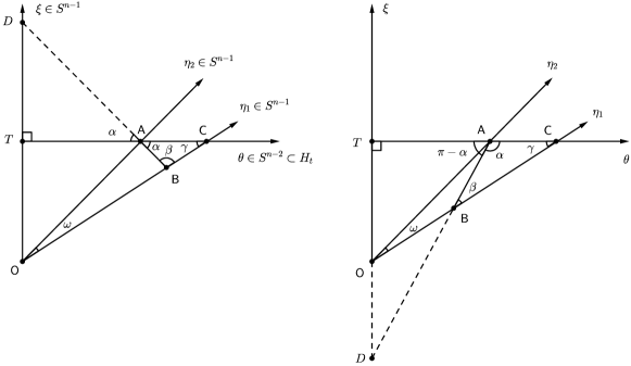
Figure 1. The diagrams represent two extremes: when the angle $\alpha$ is small $(\alpha<\pi/2)$, and when it is large $(\alpha>\pi/2)$. The point $O$ represents the origin in $\mathbb{R}^{n}$, and $\left|\overline{OT}\right|=t$ where $0\leq t\leq r/4$. The points $A$ and $C$ are the boundary points for $K$ and $K_{\delta}$ in the direction $\theta$, with two obvious possibilities: either $\left|\overline{TA}\right|=\rho_{K\cap H_{t}}(\theta)$ and $\left|\overline{TC}\right|=\rho_{K_{\delta}\cap H_{t}}(\theta)$, or the opposite. The point $B$ is a boundary point for the same convex body as $A$, but in the direction $\eta_{1}$. The point $D$ lies outside of the convex body for which $A$ and $B$ are boundary points.

Lemma (2.4) in [8] establishes the existence of a small neighbourhood of $t=0$, independent of $\xi\in S^{n-1}$, on which $A_{K,\xi}$ is $m$-smooth. The following is an elaboration of Koldobsky’s proof, so that we may uniformly approximate the derivatives of $A_{K,\xi}$. Again fix $\xi\in S^{n-1}$, and fix $\theta\in S^{n-2}\subset H_{t}$. Let $\rho_{K,\theta}$ denote the $m$-smooth restriction of $\rho_{K}$ to the two dimensional plane spanned by $\xi$ and $\theta$, and consider $\rho_{K,\theta}$ as a function on $[0,2\pi]$, where the angle is measured from the positive $\theta$-axis. A right triangle then gives the equation

$$\rho_{K\cap H_{t}}^{2}(\theta)+t^{2}=\rho_{K,\theta}^{2}\left(\arctan\left(\frac{t}{\rho_{K\cap H_{t}}(\theta)}\right)\right),$$

which we can use to implicitly differentiate $y(t):=\rho_{K\cap H_{t}}(\theta)$ as a function of $t$. Indeed,

$$F(t,y):=y^{2}+t^{2}-\rho_{K,\theta}^{2}\left(\arctan\left(\frac{t}{y}\right)\right)$$

is differentiable away from $y=0$, with

$$F_{y}(t,y)=2y+\frac{2t}{y^{2}+t^{2}}\rho_{K,\theta}\left(\arctan\left(\frac{t}{y}\right)\right)\rho_{K,\theta}^{\prime}\left(\arctan\left(\frac{t}{y}\right)\right).$$

The containment $B_{r}(0)\subset K\subset B_{R}(0)$ implies $\rho_{K,\theta}$ is bounded above on $S^{n-1}$ by $R$, and

$$\rho_{K\cap H_{t}}(\theta)\geq\frac{\sqrt{15}\,r}{4}$$

for $|t|\leq r/4$. If

$$M=1+\sup_{\xi\in S^{n-1}}\big{|}\nabla_{o}\rho_{K}(\xi)\big{|}<\infty,$$

and $\lambda\in\mathbb{R}$ is a constant such that

$$0<\lambda<\min\left\{\frac{15\sqrt{15}\,r^{3}}{128RM},\frac{r}{4}\right\},$$

then

$$\Big{|}F_{y}\big{(}t,\rho_{K\cap H_{t}}(\theta)\big{)}\Big{|}>\frac{\sqrt{15}\,r}{4}$$

for $|t|\leq\lambda$. Therefore, by the Implicit Function Theorem, $y(t)=\rho_{K\cap H_{t}}(\theta)$ is differentiable on $(-\lambda,\lambda)$, with

$$y^{\prime}(t)=\frac{\rho_{K,\theta}\left(\arctan\left(\frac{t}{y}\right)\right)\rho^{\prime}_{K,\theta}\left(\arctan\left(\frac{t}{y}\right)\right)\big{(}y^{2}+t^{2}\big{)}^{-1}y-t}{y+t\rho_{K,\theta}\left(\arctan\left(\frac{t}{y}\right)\right)\rho^{\prime}_{K,\theta}\left(\arctan\left(\frac{t}{y}\right)\right)\big{(}y^{2}+t^{2}\big{)}^{-1}}.$$

Recursion shows that $\rho_{K\cap H_{t}}(\theta)$ is $m$-smooth on $(-\lambda,\lambda)$, independent of $\xi\in S^{n-1}$ and $\theta\in S^{n-2}$. It follows from the integral expression (6) that $A_{K,\xi}$ is $m$-smooth on $(-\lambda,\lambda)$ for every $\xi\in S^{n-1}$. This argument also shows that $A_{K_{\delta},\xi}$ is $m$-smooth on the same interval, for $\delta>0$ small enough. Using the resulting expressions for the derivatives of $A_{K,\xi}$ and $A_{K_{\delta},\xi}$, and applying equations (3), (5), and the inequality (7), we have

$$\lim_{\delta\rightarrow 0}\sup_{\xi\in S^{n-1}}\sup_{|t|\leq\lambda}\left|A_{K,\xi}^{(k)}(t)-A_{K_{\delta},\xi}^{(k)}(t)\right|=0$$

for $k=1,\ldots,m$.

Finally, for any $p\in\mathbb{R}$ such that $-1<p<m$ and $p\neq 0,1,\ldots,m-1$, we will uniformly approximate $A_{K,\xi}^{(p)}(0)$. With $\lambda>0$ as chosen above, we have

$$A_{K,\xi}^{(p)}(0)= \frac{1}{\Gamma(-p)}\int_{0}^{\lambda}t^{-1-p}\left(A_{K,\xi}(-t)-\sum_{k=0}^{m-1}\frac{(-1)^{k}A_{K,\xi}^{(k)}(0)}{k!}t^{k}\right)\,dt$$

$$+\frac{1}{\Gamma(-p)}\int_{\lambda}^{\infty}t^{-1-p}A_{K,\xi}(-t)\,dt+\frac{1}{\Gamma(-p)}\sum_{k=0}^{m-1}\frac{(-1)^{k}\lambda^{k-p}A_{K,\xi}^{(k)}(0)}{k!(k-p)}.$$

The first integral in this equation can be rewritten as

$$\int_{0}^{\lambda}t^{-1-p}\int_{0}^{t}\frac{A_{K,\xi}^{(m)}(-z)}{(m-1)!}(t-z)^{m-1}\,dz\,dt,$$

using the integral form of the remainder in Taylor’s Theorem. We also have

$$\int_{\lambda}^{\infty}t^{-1-p}A_{K,\xi}(-t)\,dt$$

$$=\int_{K\cap\{\langle x,-\xi\rangle\geq\lambda\}}\langle x,-\xi\rangle^{-1-p}\,dx$$

$$=\int_{B_{K}(\xi)}\langle\eta,-\xi\rangle^{-1-p}\int_{\lambda\langle\eta,-\xi\rangle^{-1}}^{\rho_{K}(\eta)}r^{n-2-p}\,dr\,d\eta$$

$$=\frac{1}{n-1-p}\int_{B_{K}(\xi)}\Big{(}\langle\eta,-\xi\rangle^{-1-p}\rho_{K}^{n-1-p}(\eta)-\lambda^{n-1-p}\langle\eta,-\xi\rangle^{-n}\Big{)}\,d\eta,$$

where

$$B_{K}(\xi)=\Big{\{}\eta\in S^{n-1}\Big{|}\langle\eta,\xi\rangle<0\mbox{ and }\rho_{K}(\eta)\geq\lambda\langle\eta,-\xi\rangle^{-1}\Big{\}}.$$

Therefore, with the set $B_{K_{\delta}}(\xi)$ defined similarly, we have

$$\left|A_{K,\xi}^{(p)}(0)-A_{K_{\delta},\xi}^{(p)}(0)\right|\cdot\big{|}\Gamma(-p)\big{|}$$

$$\leq\frac{1}{(m-1)!}\left(\sup_{|z|\leq\lambda}\left|A_{K,\xi}^{(m)}(z)-A_{K_{\delta},\xi}^{(m)}(z)\right|\right)\int_{0}^{\lambda}\int_{0}^{t}t^{-1-p}(t-z)^{m-1}\,dz\,dt$$ (8)

$$\quad+\left(\sup_{\eta\in S^{n-1}}\left|\rho_{K}^{n-1-p}(\eta)-\rho_{K_{\delta}}^{n-1-p}(\eta)\right|\right)\int_{B_{K}(\xi)\cap B_{K_{\delta}}(\xi)}\frac{\langle\eta,-\xi\rangle^{-1-p}}{|n-1-p|}\,d\eta$$ (9)

$$\quad+\int_{B_{K}(\xi)\setminus B_{K_{\delta}}(\xi)}\left|\frac{\langle\eta,-\xi\rangle^{-1-p}\rho_{K}^{n-1-p}(\eta)-\lambda^{n-1-p}\langle\eta,-\xi\rangle^{-n}}{n-1-p}\right|\,d\eta$$ (10)

$$\quad+\int_{B_{K_{\delta}}(\xi)\setminus B_{K}(\xi)}\left|\frac{\langle\eta,-\xi\rangle^{-1-p}\rho_{K_{\delta}}^{n-1-p}(\eta)-\lambda^{n-1-p}\langle\eta,-\xi\rangle^{-n}}{n-1-p}\right|\,d\eta$$ (11)

$$\quad+\sum_{k=0}^{m-1}\frac{\lambda^{k-p}}{k!|k-p|}\left|A_{K,\xi}^{(k)}(0)-A_{K_{\delta},\xi}^{(k)}(0)\right|,$$

for $\delta>0$ small enough. The integrals in expressions (8) and (9) are finite, with

$$\int_{0}^{\lambda}\int_{0}^{t}t^{-1-p}(t-z)^{m-1}\,dz\,dt=\frac{\lambda^{m-p}}{m(m-p)},$$

since $p$ is a non-integer less than $m$, and

$$\int_{B_{K}(\xi)\cap B_{K_{\delta}}(\xi)}\langle\eta,-\xi\rangle^{-1-p}\,d\eta\leq\left(\frac{R}{\lambda}\right)^{1+p}\omega_{n}.$$

Furthermore, the integrands in expression (10) and (11) are bounded above by

$$\left(\frac{2R}{\lambda}\right)^{1+p}(2R)^{n-1-p}+\lambda^{n-1-p}\left(\frac{2R}{\lambda}\right)^{n}\qquad\mbox{ if }p<n-1,$$

and

$$\left(\frac{2R}{\lambda}\right)^{1+p}\left(\frac{r}{2}\right)^{n-1-p}+\lambda^{n-1-p}\left(\frac{2R}{\lambda}\right)^{n}\qquad\mbox{ if }p>n-1,$$

noting that $B_{r/2}(0)\subset K_{\delta}\subset B_{2R}(0)$ for $\delta<1/2$.

It is now sufficient to prove

$$\lim_{\delta\rightarrow 0}\sup_{\xi\in S^{n-1}}\int_{S^{n-1}}\chi_{B(\xi,\delta)}\,d\eta=0,$$

where

$$B(\xi,\delta)=B_{K}(\xi)\Delta B_{K_{\delta}}(\xi)$$

$$=\left\{\eta\in S^{n-1}\,\bigg{|}\,\rho_{K}(\eta)\geq\frac{\lambda}{\langle\eta,-\xi\rangle}>\rho_{K_{\delta}}(\eta)\mbox{ or }\rho_{K_{\delta}}(\eta)\geq\frac{\lambda}{\langle\eta,-\xi\rangle}>\rho_{K}(\eta)\right\}.$$

We will prove the equivalent statement

$$\lim_{\delta\rightarrow 0}\sup_{\xi\in S^{n-1}}\int_{S^{n-1}}\chi_{B(-\xi,\delta)}\,d\eta=0,$$

where the sign of $\xi$ has changed, so that we may use Figure 1.

Towards this end, fix any $\theta\in S^{n-2}$, and consider Figure 1 specifically when $t=\lambda$. In this case,

$$\left|\overline{OA}\right|=\rho_{K}(\eta_{2})=\lambda\langle\eta_{2},\xi\rangle^{-1}\mbox{ and }\left|\overline{OC}\right|=\rho_{K_{\delta}}(\eta_{1})=\lambda\langle\eta_{1},\xi\rangle^{-1}$$

or

$$\left|\overline{OC}\right|=\rho_{K}(\eta_{2})=\lambda\langle\eta_{2},\xi\rangle^{-1}\mbox{ and }\left|\overline{OA}\right|=\rho_{K_{\delta}}(\eta_{1})=\lambda\langle\eta_{1},\xi\rangle^{-1}.$$

Any $\eta\in B(-\xi,\delta)$ lying in the right half-plane spanned by $\xi$ and $\theta$ will lie between $\eta_{1}$ and $\eta_{2}$. Furthermore, the angle $\omega$ converges to zero as $\delta$ approaches zero, uniformly with respect to $\xi\in S^{n-1}$ and $\theta\in S^{n-2}$. Indeed, we have

$$0\leq\sin\omega\leq\frac{2\,\sin\beta\,\sin\gamma}{r\,\sin\alpha}\big{|}\rho_{K}(\eta_{1})-\rho_{K_{\delta}}(\eta_{1})\big{|},$$

using the fact that both $K$ and $K_{\delta}$ contain a ball of radius $r/2$, and with $\sin\alpha$ uniformly bounded away from zero as before. It follows that the spherical measure of $B(-\xi,\delta)$ converges to zero as $\delta$ approaches zero, uniformly with respect to $\xi\in S^{n-1}$. ∎

Lemma 9.

Let $K\subset\mathbb{R}^{n}$ be a convex body contained in a ball of radius $R$, and containing a ball of radius $r$, where both balls are centred at the origin. If

$$L(n)=8(n-1)\pi^{\frac{n-1}{2}}\left[\Gamma\left(\frac{n+1}{2}\right)\right]^{-1},$$

then

$$\left|A_{K,\xi}(t)-A_{K,\xi}(s)\right|\leq L(n)\,R^{n-1}\,r^{-1}\,|t-s|$$

for all $s,t\in[-r/2,r/2]$ and $\xi\in S^{n-1}$.

Proof.

For $\xi\in S^{n-1}$, Brunn’s Theorem implies $f:=A_{K,\xi}^{\frac{1}{n-1}}$ is concave on its support, which includes the interval $[-r,r]$. Let

$$L_{0}=\max\left\{\left|\frac{f\left(\frac{-3r}{4}\right)-f(-r)}{\frac{-3r}{4}-(-r)}\right|,\left|\frac{f(r)-f\left(\frac{3r}{4}\right)}{r-\frac{3r}{4}}\right|\right\},$$

and suppose $s,t\in[-r/2,r/2]$ are such that $s<t$. If

$$\frac{f(t)-f(s)}{t-s}>0,$$

then

$$\frac{f\left(\frac{-3r}{4}\right)-f(-r)}{\frac{-3r}{4}-(-r)}\geq\frac{f(s)-f\left(\frac{-3r}{4}\right)}{s-\left(\frac{-3r}{4}\right)}\geq\frac{f(t)-f(s)}{t-s}>0\,;$$

otherwise, we will obtain a contradiction of the concavity of $f$. Similarly, if

$$\frac{f(t)-f(s)}{t-s}<0,$$

then

$$\frac{f(r)-f\left(\frac{3r}{4}\right)}{r-\frac{3r}{4}}\leq\frac{f\left(\frac{3r}{4}\right)-f(t)}{\frac{3r}{4}-t}\leq\frac{f(t)-f(s)}{t-s}<0.$$

Therefore,

$$\left|A_{K,\xi}^{\frac{1}{n-1}}(t)-A_{K,\xi}^{\frac{1}{n-1}}(s)\right|\leq L_{0}\,|t-s|$$

for all $s,t\in[-r/2,r/2]$. Now, we have

$$\left|A_{K,\xi}(t)-A_{K,\xi}(s)\right| \leq(n-1)\left(\max_{t_{0}\in\mathbb{R}}A_{K,\xi}(t_{0})\right)^{\frac{n-2}{n-1}}\left|A_{K,\xi}^{\frac{1}{n-1}}(t)-A_{K,\xi}^{\frac{1}{n-1}}(s)\right|$$

by the Mean Value Theorem, and

$$L_{0} \leq\frac{4}{r}\cdot 2\left(\max_{t_{0}\in\mathbb{R}}A_{K,\xi}(t_{0})\right)^{\frac{1}{n-1}}=\frac{8}{r}A_{K,\xi}^{\frac{1}{n-1}}\big{(}t_{K}(\xi)\big{)}.$$

Finally, since $K$ is contained in a ball of radius $R$, we have

$$A_{K,\xi}\big{(}t_{K}(\xi)\big{)}\leq\frac{\pi^{\frac{n-1}{2}}}{\Gamma\left(\frac{n+1}{2}\right)}R^{n-1}.$$

Combining these inequalities gives

$$\left|A_{K,\xi}(t)-A_{K,\xi}(s)\right|\leq L(n)\,R^{n-1}\,r^{-1}\,|t-s|$$

for all $s,t\in[-r/2,r/2]$ and $\xi\in S^{n-1}$. ∎

We now prove two lemmas that will be the core of the proof of Theorem 2.

Lemma 10.

Let $K$ be a convex body in $\mathbb{R}^{n}$ contained in a ball of radius $R$, and containing a ball of radius $r$, where both balls are centred at the origin. Let $\{K_{\delta}\}_{0<\delta<1}$ be as in Lemma 8. If there exists $0<\varepsilon<\frac{r^{2}}{16}$ so that

$$\rho(CK,IK)\leq\varepsilon,$$

then, for $\delta>0$ small enough,

$$\int_{S^{1}}\big{|}A_{K_{\delta},\xi}^{\prime}(0)\big{|}\,d\xi\leq\left(6\pi+\frac{32\,\pi}{\sqrt{3}\,r}\right)\sqrt{\varepsilon}\ \mbox{ when }n=2,$$

$$\int_{S^{n-1}}\big{|}A_{K_{\delta},\xi}^{\prime}(0)\big{|}^{2}\,d\xi\leq C(n)\left(\sqrt{\varepsilon}+\frac{R^{2n-4}}{r}+\frac{R^{3n-3}}{r^{n+2}}\right)\sqrt{\varepsilon}\ \mbox{ when }n\geq 3.$$

Here, $C(n)>0$ are constants depending only on the dimension.

Proof.

By Lemma 8, we may choose $0<\alpha<1/2$ small enough so that for every $0<\delta<\alpha$,

$$\sup_{\xi\in S^{n-1}}\sup_{|t|\leq r/4}\big{|}A_{K,\xi}(t)-A_{K_{\delta},\xi}(t)\big{|}\leq\varepsilon.$$

We first show that for each $0<\delta<\alpha$ and $\xi\in S^{n-1}$, there exists a number $c_{\delta}(\xi)$ with $|c_{\delta}(\xi)|\leq\sqrt{\varepsilon}$ for which

$$\big{|}A_{K_{\delta},\xi}^{\prime}\big{(}c_{\delta}(\xi)\big{)}\big{|}\leq 3\sqrt{\varepsilon}.$$

Indeed, if $\xi\in S^{n-1}$ is such that $|t_{K_{\delta}}(\xi)|\leq\sqrt{\varepsilon}$, then

$$A_{K_{\delta},\xi}^{\prime}\big{(}t_{K_{\delta}}(\xi)\big{)}=0,$$

and we may take $c_{\delta}(\xi)=t_{K_{\delta}}(\xi)$.

Assume $\xi\in S^{n-1}$ is such that $|t_{K_{\delta}}(\xi)|>\sqrt{\varepsilon}$. Letting $s$ denote the sign of $t_{K_{\delta}}(\xi)$, we have

$$\big{|}A_{K_{\delta},\xi}(s\sqrt{\varepsilon})-A_{K_{\delta},\xi}(0)\big{|}=A_{K_{\delta},\xi}(s\sqrt{\varepsilon})-A_{K_{\delta},\xi}(0)$$

$$=\Big{(}A_{K,\xi}(s\sqrt{\varepsilon})-A_{K,\xi}(0)\Big{)}+\Big{(}A_{K_{\delta},\xi}(s\sqrt{\varepsilon})-A_{K,\xi}(s\sqrt{\varepsilon})\Big{)}$$

$$\hskip 128.0374pt+\Big{(}A_{K,\xi}(0)-A_{K_{\delta},\xi}(0)\Big{)}$$

$$\leq\sup_{\xi\in S^{n-1}}\left|\max_{t\in\mathbb{R}}A_{K,\xi}(t)-A_{K,\xi}(0)\right|+2\sup_{\xi\in S^{n-1}}\sup_{|t|\leq r/4}\big{|}A_{K,\xi}(t)-A_{K_{\delta},\xi}(t)\big{|}$$

$$\leq 3\varepsilon.$$

It then follows from the Mean Value Theorem that there is a number $c_{\delta}(\xi)$ with $|c_{\delta}(\xi)|\leq\sqrt{\varepsilon}$ for which

$$\big{|}A_{K_{\delta},\xi}^{\prime}\big{(}c_{\delta}(\xi)\big{)}\big{|}=\left|\frac{A_{K_{\delta},\xi}(s\sqrt{\varepsilon})-A_{K_{\delta},\xi}(0)}{\sqrt{\varepsilon}-0}\right|\leq 3\sqrt{\varepsilon}.$$

With the numbers $c_{\delta}(\xi)$ as above, for the case $n=2$ we have

$$\int_{S^{1}}\big{|}A_{K_{\delta},\xi}^{\prime}(0)\big{|}\,d\xi$$

$$\leq\int_{S^{1}}\left(\big{|}A_{K_{\delta},\xi}^{\prime}\big{(}c_{\delta}(\xi)\big{)}\big{|}+\left|\int_{c_{\delta}(\xi)}^{0}A_{K_{\delta},\xi}^{\prime\prime}(t)\,dt\right|\right)\,d\xi$$

$$\leq 6\pi\sqrt{\varepsilon}+\int_{S^{1}}\int_{-\sqrt{\varepsilon}}^{\sqrt{\varepsilon}}\big{|}A_{K_{\delta},\xi}^{\prime\prime}(t)\big{|}\,dt\,d\xi.$$ (12)

When $0<\delta<1/2$, $K_{\delta}$ is contained in a ball of radius $2R$, and contains a ball of radius $r/2$. Lemma 9 then implies

$$\sup_{\xi\in S^{n-1}}\sup_{t\in(-\sqrt{\varepsilon},\sqrt{\varepsilon})}\big{|}A_{K_{\delta},\xi}^{\prime}(t)\big{|}\leq\frac{2L(n)\,(2R)^{n-1}}{r}.$$

So, when $n\geq 3$,

$$\int_{S^{n-1}}\big{|}A_{K_{\delta},\xi}^{\prime}(0)\big{|}^{2}\,d\xi$$

$$\leq\int_{S^{n-1}}\left(\big{|}A_{K_{\delta},\xi}^{\prime}\big{(}c_{\delta}(\xi)\big{)}\big{|}^{2}+\left|\int_{c_{\delta}(\xi)}^{0}2A_{K_{\delta},\xi}^{\prime\prime}(t)A_{K_{\delta},\xi}^{\prime}(t)\,dt\right|\right)\,d\xi$$

$$\leq 9\,\omega_{n}\,\varepsilon+\frac{4L(n)\,(2R)^{n-1}}{r}\int_{S^{n-1}}\int_{-\sqrt{\varepsilon}}^{\sqrt{\varepsilon}}\big{|}A_{K_{\delta},\xi}^{\prime\prime}(t)\big{|}\,dt\,d\xi$$ (13)

Considering inequalities (3) and (3), we still need to bound

$$\int_{S^{n-1}}\int_{-\sqrt{\varepsilon}}^{\sqrt{\varepsilon}}\big{|}A_{K_{\delta},\xi}^{\prime\prime}(t)\big{|}\,dt\,d\xi$$

for arbitrary $n$. Rearranging the equation

$$\frac{d^{2}}{dt^{2}}A_{K_{\delta},\xi}^{\frac{1}{n-1}}(t) =\frac{d}{dt}\left(\frac{1}{n-1}A_{K_{\delta},\xi}^{\frac{2-n}{n-1}}(t)\,A_{K_{\delta},\xi}^{\prime}(t)\right)$$

$$=\frac{2-n}{(n-1)^{2}}A_{K_{\delta},\xi}^{\frac{3-2n}{n-1}}(t)\,\left(A_{K_{\delta},\xi}^{\prime}(t)\right)^{2}+\frac{1}{n-1}A_{K_{\delta},\xi}^{\frac{2-n}{n-1}}(t)\,A_{K_{\delta},\xi}^{\prime\prime}(t)$$

gives

$$A_{K_{\delta},\xi}^{\prime\prime}(t)=(n-1)A_{K_{\delta},\xi}^{\frac{n-2}{n-1}}(t)\frac{d^{2}}{dt^{2}}A_{K_{\delta},\xi}^{\frac{1}{n-1}}(t)+\frac{n-2}{n-1}\frac{\big{(}A_{K_{\delta},\xi}^{\prime}(t)\big{)}^{2}}{A_{K_{\delta},\xi}(t)}.$$

Brunn’s Theorem implies that the second derivative of $A_{K_{\delta},\xi}^{\frac{1}{n-1}}$ is non-positive for $|t|<r$, so

$$\big{|}A_{K_{\delta},\xi}^{\prime\prime}(t)\big{|} \leq(1-n)A_{K_{\delta},\xi}^{\frac{n-2}{n-1}}(t)\frac{d^{2}}{dt^{2}}A_{K_{\delta},\xi}^{\frac{1}{n-1}}(t)+\frac{n-2}{n-1}\frac{\big{(}A_{K_{\delta},\xi}^{\prime}(t)\big{)}^{2}}{A_{K_{\delta},\xi}(t)}$$

$$=-A_{K_{\delta},\xi}^{\prime\prime}(t)+2\left(\frac{n-2}{n-1}\right)\frac{\big{(}A_{K_{\delta},\xi}^{\prime}(t)\big{)}^{2}}{A_{K_{\delta},\xi}(t)}.$$

Because $K_{\delta}$ contains a ball of radius $r/2$ centred at the origin, we have

$$A_{K_{\delta},\xi}(t)\geq\frac{1}{\Gamma\left(\frac{n+1}{2}\right)}\left(\frac{3\pi r^{2}}{16}\right)^{\frac{n-1}{2}}$$

for $|t|\leq r/4$, and so

$$\frac{n-2}{n-1}\frac{\big{(}A_{K_{\delta},\xi}^{\prime}(t)\big{)}^{2}}{A_{K_{\delta},\xi}(t)} \leq\frac{n-2}{n-1}\,\Gamma\left(\frac{n+1}{2}\right)\,\left(\frac{2L(n)\,(2R)^{n-1}}{r}\right)^{2}\,\left(\frac{16}{3\pi r^{2}}\right)^{\frac{n-1}{2}}$$

$$=\frac{\widetilde{L}(n)\,R^{2n-2}}{r^{n+1}}$$

for all $|t|\leq\sqrt{\varepsilon}$, where $\widetilde{L}(n)$ is a constant depending only on $n$. Therefore,

$$\int_{S^{n-1}}\int_{-\sqrt{\varepsilon}}^{\sqrt{\varepsilon}}\Big{|}A_{K_{\delta},\xi}^{\prime\prime}(t)\Big{|}\,dt\,d\xi$$

$$\leq\int_{S^{n-1}}\int_{-\sqrt{\varepsilon}}^{\sqrt{\varepsilon}}\Big{(}-A_{K_{\delta},\xi}^{\prime\prime}(t)\Big{)}\,dt\,d\xi+\frac{4\,\omega_{n}\,\widetilde{L}(n)\,R^{2n-2}}{r^{n+1}}\sqrt{\varepsilon}.$$ (14)

We will bound the first term on the final line above using formula (1). Letting

$$\widetilde{C}(n)=\frac{\Gamma\left(\frac{n}{2}\right)}{\sqrt{\pi}\,\Gamma\left(\frac{n-1}{2}\right)},$$

formula (1) becomes

$$f_{K_{\delta}}(t) =\widetilde{C}(n)\int_{S^{n-1}}\int_{|t|}^{\rho_{K_{\delta}}(\xi)}\frac{1}{r}\left(1-\frac{t^{2}}{r^{2}}\right)^{\frac{n-3}{2}}r^{n-1}\,dr\,d\xi$$

$$=\widetilde{C}(n)\int_{S^{n-1}}\int_{|t|}^{\rho_{K_{\delta}}(\xi)}r\left(r^{2}-t^{2}\right)^{\frac{n-3}{2}}\,dr\,d\xi$$

$$=\frac{\widetilde{C}(n)}{(n-1)}\int_{S^{n-1}}\left(\rho_{K_{\delta}}^{2}(\xi)-t^{2}\right)^{\frac{n-1}{2}}\,d\xi.$$

The derivatives of $A_{K_{\delta},\xi}$ and $\left(\rho_{K_{\delta}}^{2}(\xi)-t^{2}\right)^{\frac{n-1}{2}}$ are bounded on $(-\sqrt{\varepsilon},\sqrt{\varepsilon})$ uniformly with respect to $\xi\in S^{n-1}$, so

$$f_{K_{\delta}}^{\prime}(t)=\frac{1}{\omega_{n}}\int_{S^{n-1}}A_{K_{\delta},\xi}^{\prime}(t)\,d\xi=-\widetilde{C}(n)\,t\int_{S^{n-1}}\left(\rho_{K_{\delta}}^{2}(\xi)-t^{2}\right)^{\frac{n-3}{2}}\,d\xi.$$

Observing $\widetilde{C}(2)=\pi^{-1}$, and using that $0<\varepsilon<r^{2}/16$ and $r/2\leq\rho_{K_{\delta}}\leq 2R$ for $\delta<1/2$, we have

$$\left|\int_{S^{n-1}}A_{K_{\delta},\xi}^{\prime}(\pm\sqrt{\varepsilon})\,d\xi\right|$$

$$=\omega_{n}\left|f_{K_{\delta}}^{\prime}(\pm\sqrt{\varepsilon})\right|=\widetilde{C}(n)\,\omega_{n}\sqrt{\varepsilon}\int_{S^{n-1}}\left(\rho_{K_{\delta}}^{2}(\xi)-\varepsilon\right)^{\frac{n-3}{2}}\,d\xi$$

$$\leq\begin{cases}16\,\pi\left(\sqrt{3}\,r\right)^{-1}\sqrt{\varepsilon}\ &\mbox{ if }n=2,\\ \widetilde{C}(n)\,\omega_{n}^{2}\,(2R)^{n-3}\sqrt{\varepsilon}\ &\mbox{ if }n\geq 3.\end{cases}$$

This implies

$$\left|\int_{S^{n-1}}\int_{-\sqrt{\varepsilon}}^{\sqrt{\varepsilon}}-A_{K_{\delta},\xi}^{\prime\prime}(t)\,dt\,d\xi\right| =\left|\int_{S^{n-1}}\big{(}A_{K_{\delta},\xi}^{\prime}(-\sqrt{\varepsilon})-A_{K_{\delta},\xi}^{\prime}(\sqrt{\varepsilon})\big{)}\,d\xi\right|$$

$$\leq\begin{cases}32\,\pi\left(\sqrt{3}\,r\right)^{-1}\sqrt{\varepsilon}\ &\mbox{ if }n=2,\\ 2\,\widetilde{C}(n)\,\omega_{n}^{2}\,(2R)^{n-3}\sqrt{\varepsilon}\ &\mbox{ if }n\geq 3.\end{cases}$$ (15)

Noting that $\widetilde{L}(2)=0$, inequalities (3), (3), and (3) give

$$\int_{S^{1}}\big{|}A_{K_{\delta},\xi}^{\prime}(0)\big{|}\,d\xi\leq\left(6\pi+\frac{32\pi}{\sqrt{3}\,r}\right)\sqrt{\varepsilon}$$

when $n=2$. For $n\geq 3$, inequalities (3), (3), and (3) give

$$\int_{S^{n-1}}\big{|}A_{K_{\delta},\xi}^{\prime}(0)\big{|}^{2}\,d\xi\leq C(n)\left(\sqrt{\varepsilon}+\frac{R^{2n-4}}{r}+\frac{R^{3n-3}}{r^{n+2}}\right)\sqrt{\varepsilon},$$

where $C(n)$ is a constant depending on $n$. ∎

Lemma 11.

Let $K$ and $L$ be infinitely smooth convex bodies in $\mathbb{R}^{n}$ which are contained in a ball of radius $R$, and contain a ball of radius $r$, where both balls are centred at the origin. Let $p\in(0,n)$. If $\varepsilon>0$ is such that

$$\left\|I_{p}\left(\|\xi\|_{K}^{-n+p}-\|\xi\|_{L}^{-n+p}\right)\right\|_{2}\leq\varepsilon,$$

then when $n\leq 2p$,

$$\rho(K,L)\leq C(n,p)\,R^{2}r^{\frac{-3n-1+2p}{n+1}}\varepsilon^{\frac{2}{n+1}},$$

and when $n>2p$,

$$\rho(K,L)\leq C(n,p)\,R^{2}r^{\frac{-3n-1+2p}{n+1}}\left(\varepsilon^{2}+\frac{R^{2(n+1-p)}}{r^{2}}\right)^{\frac{n-2p}{(n+2-2p)(n+1)}}\varepsilon^{\frac{4}{(n+2-2p)(n+1)}}.$$

Here, $\|\cdot\|_{2}$ denotes the norm on $L^{2}(S^{n-1})$, and $C(n,p)>0$ are constants depending on the dimension and $p$.

Proof.

Define the function

$$f(\xi):=\|\xi\|_{K}^{-n+p}-\|\xi\|_{L}^{-n+p}$$

on $S^{n-1}$. Towards bounding the radial distance between $K$ and $L$ by $\|f\|_{2}$, the $L^{2}(S^{n-1})$ norm of $f$, note that the identity

$$\rho_{K}(\xi)-\rho_{L}(\xi)=\rho_{K}(\xi)\rho_{L}(\xi)\big{(}\|\xi\|_{L}-\|\xi\|_{K}\big{)}$$

implies

$$\big{|}\rho_{K}(\xi)-\rho_{L}(\xi)\big{|}\leq R^{2}\big{|}\|\xi\|_{K}-\|\xi\|_{L}\big{|}.$$

By Theorem 6, we have

$$\delta_{\infty}(K^{\circ},L^{\circ})\leq C(n)D^{\frac{n-1}{n+1}}\big{(}\delta_{2}(K^{\circ},L^{\circ})\big{)}^{\frac{2}{n+1}},$$

where $C(n)>0$ is a constant depending on $n$, and $D$ is the diameter of $K^{\circ}\cup L^{\circ}$. Both $K^{\circ}$ and $L^{\circ}$ are contained in a ball of radius $r^{-1}$ centred at the origin. We then have $D\leq 2r^{-1}$, and

$$\sup_{\xi\in S^{n-1}}\big{|}\|\xi\|_{K}-\|\xi\|_{L}\big{|}\leq C(n)r^{\frac{1-n}{n+1}}\left(\int_{S^{n-1}}\big{(}\|\xi\|_{K}-\|\xi\|_{L}\big{)}^{2}\,d\xi\right)^{\frac{1}{n+1}}$$

for some new constant $C(n)$. There exists a function $g:S^{n-1}\rightarrow\mathbb{R}$ such that

$$\big{(}\|\xi\|_{K}-\|\xi\|_{L}\big{)}g(\xi)=\|\xi\|_{K}^{-n+p}-\|\xi\|_{L}^{-n+p}.$$

If $\xi\in S^{n-1}$ is such that $\|\xi\|_{K}\neq\|\xi\|_{L}$, then an application of the Mean Value Theorem to the function $t^{-n+p}$ on the interval bounded by $\|\xi\|_{K}$ and $\|\xi\|_{L}$ gives

$$|g(\xi)|\geq(n-p)\left(\max\big{\{}\|\xi\|_{K},\|\xi\|_{L}\big{\}}\right)^{-n-1+p}\geq(n-p)r^{n+1-p}.$$

Therefore,

$$\big{|}\|\xi\|_{K}-\|\xi\|_{L}\big{|}\leq(n-p)^{-1}r^{-n-1+p}|f(\xi)|.$$

Combining the above inequalities, we get

$$\sup_{\xi\in S^{n-1}}\big{|}\rho_{K}(\xi)-\rho_{L}(\xi)\big{|}\leq C(n,p)R^{2}r^{\frac{-3n-1+2p}{n+1}}\|f\|_{2}^{\frac{2}{n+1}},$$ (16)

for some constant $C(n,p)$.

We now compare the $L^{2}$ norm of $f$ to that of $I_{p}(f)$ by considering two separate cases based on the dimension $n$, as in the proof of Theorem 3.6 in [6]. In both cases, we let $\sum_{m=0}^{\infty}Q_{m}$ be the condensed harmonic expansion for $f$, and let $\lambda_{m}(n,p)$ be the eigenvalues from Lemma 7. As in [6], the condensed harmonic expansion for $I_{p}f$ is then given by $\sum_{m=0}^{\infty}\lambda_{m}(n,p)Q_{m}$.

Assume $n\leq 2p$. An application of Stirling’s formula to the equations given in Lemma 7 shows that $\lambda_{m}(n,p)$ diverges to infinity as $m$ approaches infinity. The eigenvalues are also non-zero, so there is a constant $C(n,p)$ such that $C(n,p)|\lambda_{m}(n,p)|^{2}$ is greater than one for all $m$. Therefore,

$$\|f\|_{2}^{2} =\sum_{m=0}^{\infty}\|Q_{m}\|_{2}^{2}$$

$$\leq C(n,p)\sum_{m=0}^{\infty}\big{|}\lambda_{m}(n,p)\big{|}^{2}\|Q_{m}\|_{2}^{2}=C(n,p)\|I_{p}(f)\|_{2}^{2}\leq C(n,p)\varepsilon^{2}.$$

Combining this inequality with (16) gives the first estimate in the theorem.

Assume $n>2p$. Hölder’s inequality gives

$$\|f\|_{2}^{2}=\sum_{m=0}^{\infty}\|Q_{m}\|_{2}^{2}$$

$$=\sum_{m=0}^{\infty}\left(\big{|}\lambda_{m}(n,p)\big{|}^{\frac{4}{n+2-2p}}\left\|Q_{m}\right\|_{2}^{\frac{4}{n+2-2p}}\right)\cdot\left(\big{|}\lambda_{m}(n,p)\big{|}^{\frac{-4}{n+2-2p}}\left\|Q_{m}\right\|_{2}^{\frac{2n-4p}{n+2-2p}}\right)$$

$$\leq\left(\sum_{m=0}^{\infty}\big{|}\lambda_{m}(n,p)\big{|}^{2}\left\|Q_{m}\right\|_{2}^{2}\right)^{\frac{2}{n+2-2p}}\left(\sum_{m=0}^{\infty}\big{|}\lambda_{m}(n,p)\big{|}^{\frac{-4}{n-2p}}\left\|Q_{m}\right\|_{2}^{2}\right)^{\frac{n-2p}{n+2-2p}},$$

where we again note that the eigenvalues are all non-zero. It follows from Lemma 7 and Stirling’s formula that there is a constant $C(n,p)$ such that

$$\big{|}\lambda_{m}(n,p)\big{|}^{\frac{-4}{n-2p}}\leq C(n,p)m^{2}$$

for all $m\geq 1$, and

$$\big{|}\lambda_{0}(n,p)\big{|}^{\frac{-4}{n-2p}}\leq C(n,p).$$

Using the identity

$$\|\nabla_{o}f\|_{2}^{2}=\sum_{m=1}^{\infty}m(m+n-2)\|Q_{m}\|_{2}^{2}$$ (17)

given by Corollary 3.2.12 in [7], we then have

$$\|f\|_{2}^{2} \leq C(n,p)\left(\left\|I_{p}(f)\right\|_{2}^{2}\right)^{\frac{2}{n+2-2p}}\left(\|Q_{0}\|_{2}^{2}+\|\nabla_{o}f\|_{2}^{2}\right)^{\frac{n-2p}{n+2-2p}}.$$

The Minkowski functional of a convex body is the support function of the corresponding polar body, so

$$\nabla_{o}\|\xi\|_{K}^{-n+p}=(-n+p)\|\xi\|_{K}^{-n-1+p}\,\nabla_{o}h_{K^{\circ}}(\xi).$$

Because $K^{\circ}$ is contained in a ball of radius $r^{-1}$, it follows from Lemma 2.2.1 in [7] that

$$|\nabla_{o}h_{K^{\circ}}(\xi)|\leq 2r^{-1}$$

for all $\xi\in S^{n-1}$. We now have

$$\left\|\nabla_{o}\|\xi\|_{K}^{-n+p}\right\|_{2}^{2}\leq 4(n-p)^{2}R^{2(n+1-p)}r^{-2}\omega_{n}.$$

This constant bounds the squared $L^{2}$ norm of $\nabla_{o}\|\xi\|_{L}^{-n+p}$ as well, so

$$\big{\|}\nabla_{o}f\big{\|}_{2}^{2} \leq 16(n-p)^{2}R^{2(n+1-p)}r^{-2}\omega_{n}.$$

Therefore,

$$\|f\|_{2}^{2}\leq C(n,p)\varepsilon^{\frac{4}{n+2-2p}}\left(\varepsilon^{2}+R^{2(n+1-p)}r^{-2}\right)^{\frac{n-2p}{n+2-2p}},$$

where the constant $C(n,p)>0$ is different from before. This inequality with (16) gives the second estimate in the theorem. ∎

4. Proofs of Stability Results

We are now ready to prove our stability results.

Proof of Theorem 2.

Let $\{K_{\delta}\}_{0<\delta<1}$ be the family of smooth convex bodies from Lemma 8. We will show that $\rho(K_{\delta},-K_{\delta})$ is small for $0<\delta<\alpha$, where $\alpha$ is the constant from the proof of Lemma 10. The bounds in the theorem will then follow from

$$\rho(K,-K)\leq\lim_{\delta\rightarrow 0}\big{(}2\rho(K,K_{\delta})+\rho(K_{\delta},-K_{\delta})\big{)}=\lim_{\delta\rightarrow 0}\rho(K_{\delta},-K_{\delta}).$$

We begin by separately considering the case $n=2$. Let the radial function $\rho_{K_{\delta}}$ be a function of the angle measured counter-clockwise from the positive horizontal axis. For any $\xi\in S^{1}$, let the angles $\phi_{1}$ and $\phi_{2}$ be functions of $t\in(-r,r)$ as indicated in Figure 2. If $\xi$ corresponds to the angle $\theta$, then the parallel section function for $K_{\delta}$ may be written as

$$A_{K_{\delta},\theta}(t)=\rho_{K_{\delta}}(\theta+\phi_{1})\,\sin\phi_{1}+\rho_{K_{\delta}}(\theta-\phi_{2})\,\sin\phi_{2}.$$

Implicit differentiation of

$$\cos\phi_{j}=\frac{t}{\rho_{K_{\delta}}\left(\theta-(-1)^{j}\phi_{j}\right)}\ \ (j=1,2)$$

gives

$$\frac{d\phi_{j}}{dt}\Big{|}_{t=0}=\frac{(-1)}{\rho_{K_{\delta}}\left(\theta-(-1)^{j}\frac{\pi}{2}\right)},$$

so

$$A_{K_{\delta},\theta}^{\prime}(0)=-\frac{\rho_{K_{\delta}}^{\prime}\left(\theta+\frac{\pi}{2}\right)}{\rho_{K_{\delta}}\left(\theta+\frac{\pi}{2}\right)}+\frac{\rho_{K_{\delta}}^{\prime}\left(\theta-\frac{\pi}{2}\right)}{\rho_{K_{\delta}}\left(\theta-\frac{\pi}{2}\right)}.$$

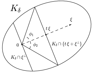
Figure 2. $K_{\delta}$ is a convex body in $\mathbb{R}^{2}$, and $\xi\in S^{1}$.

Since $f(\phi):=\rho_{K_{\delta}}(\phi+\pi/2)-\rho_{K_{\delta}}(\phi-\pi/2)$ is a continuous function on $[0,\pi]$ with

$$f(0)=\rho_{K_{\delta}}(\pi/2)-\rho_{K_{\delta}}(-\pi/2)=-\big{(}\rho_{K_{\delta}}(-\pi/2)-\rho_{K_{\delta}}(\pi/2)\big{)}=-f(\pi),$$

there exists an angle $\theta_{0}\in[0,\pi]$ such that $\rho_{K_{\delta}}(\theta_{0}+\pi/2)=\rho_{K_{\delta}}(\theta_{0}-\pi/2)$. With this $\theta_{0}$, we get the inequality

$$\left|\int_{\theta_{0}}^{\theta}\left(-\frac{\rho_{K_{\delta}}^{\prime}\left(\phi+\frac{\pi}{2}\right)}{\rho_{K_{\delta}}\left(\phi+\frac{\pi}{2}\right)}+\frac{\rho_{K_{\delta}}^{\prime}\left(\phi-\frac{\pi}{2}\right)}{\rho_{K_{\delta}}\left(\phi-\frac{\pi}{2}\right)}\right)\,d\phi\right|\leq\int_{0}^{2\pi}\left|A_{K_{\delta},\phi}^{\prime}(0)\right|\,d\phi.$$

Integrating the left side of this inequality, and applying Lemma 10 to the right side, gives

$$\left|\log\left(\frac{\rho_{K_{\delta}}\left(\theta-\frac{\pi}{2}\right)}{\rho_{K_{\delta}}\left(\theta+\frac{\pi}{2}\right)}\right)\right|\leq\left(6\pi+\frac{32\pi}{\sqrt{3}\,r}\right)\sqrt{\varepsilon}.$$

This implies

$$1-\exp\left[\left(6\pi+\frac{32\pi}{\sqrt{3}\,r}\right)\sqrt{\varepsilon}\right] \leq\exp\left[-\left(6\pi+\frac{32\pi}{\sqrt{3}\,r}\right)\sqrt{\varepsilon}\right]-1$$

$$\leq\frac{\rho_{K_{\delta}}\left(\theta-\frac{\pi}{2}\right)}{\rho_{K_{\delta}}\left(\theta+\frac{\pi}{2}\right)}-1$$

$$\leq\exp\left[\left(6\pi+\frac{32\pi}{\sqrt{3}\,r}\right)\ \sqrt{\varepsilon}\right]-1.$$

It follows that

$$-2\left(\exp\left[\left(6\pi+\frac{32\pi}{\sqrt{3}\,r}\right)\sqrt{\varepsilon}\right]-1\right)R \leq\rho_{K_{\delta}}\left(\theta-\frac{\pi}{2}\right)-\rho_{K_{\delta}}\left(\theta+\frac{\pi}{2}\right)$$

$$\leq 2\left(\exp\left[\left(6\pi+\frac{32\pi}{\sqrt{3}\,r}\right)\sqrt{\varepsilon}\right]-1\right)R,$$

since $K_{\delta}$ is contained in a ball of radius $2R$. Viewing $\rho_{K_{\delta}}$ again as a function of vectors, we have

$$\sup_{\xi\in S^{1}}\left|\rho_{K_{\delta}}(\xi)-\rho_{K_{\delta}}(-\xi)\right|\leq 2\left(\exp\left[\left(6\pi+\frac{32\pi}{\sqrt{3}\,r}\right)\sqrt{\varepsilon}\right]-1\right)R.$$

The inequality $e^{t}-1\leq 2t$ is valid when $0<t<1$; therefore, if

$$\varepsilon<\left(\frac{\sqrt{3}\,r}{6\sqrt{3}\pi r+32\pi}\right)^{2},$$

then

$$\sup_{\xi\in S^{1}}\left|\rho_{K_{\delta}}(\xi)-\rho_{K_{\delta}}(-\xi)\right|\leq\left(24\pi+\frac{128\pi}{\sqrt{3}\,r}\right)R\sqrt{\varepsilon}.$$

Consider the case when $n>2$. For $K_{\delta}$ with $p=1$, Equation (2) becomes

$$I_{2}\left(\|x\|_{K_{\delta}}^{-n+2}-\|-x\|_{K_{\delta}}^{-n+2}\right)(\xi)=-2\pi i\,(n-2)A_{K_{\delta},\xi}^{\prime}(0),$$

so

$$\left\|I_{2}\left(\|x\|_{K_{\delta}}^{-n+2}-\|x\|_{-K_{\delta}}^{-n+2}\right)\right\|_{2}=2\pi(n-2)\left(\int_{S^{n-1}}\big{|}A_{K_{\delta},\xi}^{\prime}(0)\big{|}^{2}\,d\xi\right)^{\frac{1}{2}}$$

$$\leq\widetilde{C}(n)\left(\sqrt{\varepsilon}+\frac{R^{2n-4}}{r}+\frac{R^{3n-3}}{r^{n+2}}\right)^{\frac{1}{2}}\varepsilon^{\frac{1}{4}}$$

by Lemma 10. Finally, by Lemma 11,

$$\rho(K_{\delta},-K_{\delta})\leq C(n)\frac{R^{2}}{r^{\frac{3n-3}{n+1}}}\left(\sqrt{\varepsilon}+\frac{R^{2n-4}}{r}+\frac{R^{3n-3}}{r^{n+2}}\right)^{\frac{1}{n+1}}\varepsilon^{\frac{1}{2(n+1)}}$$

when $n=3\mbox{ or }4$, and

$$\rho(K_{\delta},-K_{\delta})\leq C(n) \left[\left(\sqrt{\varepsilon}+\frac{R^{2n-4}}{r}+\frac{R^{3n-3}}{r^{n+2}}\right)\sqrt{\varepsilon}+\frac{R^{2(n-1)}}{r^{2}}\right]^{\frac{n-4}{(n-2)(n+1)}}$$

$$\cdot\left(\sqrt{\varepsilon}+\frac{R^{2n-4}}{r}+\frac{R^{3n-3}}{r^{n+2}}\right)^{\frac{2}{(n-2)(n+1)}}\frac{R^{2}\varepsilon^{\frac{1}{(n-2)(n+1)}}}{r^{\frac{3n-3}{n+1}}}$$

when $n\geq 5$, where $C(n)>0$ are constants depending on the dimension. ∎

We now present the proof of our second stability result.

Proof of Theorem 5.

Apply Lemma 8 to $K$ and $L$; let $\{K_{\delta}\}_{0<\delta<1}$ and $\{L_{\delta}\}_{0<\delta<1}$ be the resulting families of smooth convex bodies. For each $\delta$, define the constant

$$\varepsilon_{\delta}:=\sup_{\xi\in S^{n-1}}\left|A_{K_{\delta},\xi}^{(p)}(0)-A_{K,\xi}^{(p)}(0)\right|+\sup_{\xi\in S^{n-1}}\left|A_{L_{\delta},\xi}^{(p)}(0)-A_{L,\xi}^{(p)}(0)\right|+\varepsilon.$$

Defining the auxiliary function

$$f_{\delta}(\xi):=\|\xi\|_{K_{\delta}}^{-n+1+p}-\|\xi\|_{L_{\delta}}^{-n+1+p},$$

we have

$$\cos\left(\frac{p\pi}{2}\right)I_{1+p}\big{(}f_{\delta}(x)+f_{\delta}(-x)\big{)}(\xi)+i\sin\left(\frac{p\pi}{2}\right)I_{1+p}\big{(}f_{\delta}(x)-f_{\delta}(-x)\big{)}(\xi)$$

$$=2\pi(n-1-p)\Big{(}A_{K_{\delta},\,\xi}^{(p)}(0)-A_{L_{\delta},\,\xi}^{(p)}(0)\Big{)}$$

from Equation (2). The function of $\xi$ on the left side of this equality is split into its even and odd parts, because $I_{1+p}$ preserves even and odd symmetry. Therefore,

$$\frac{\cos\left(\frac{p\pi}{2}\right)}{\pi(n-1-p)}I_{1+p}\big{(}f_{\delta}(x)+f_{\delta}(-x)\big{)}(\xi)$$

$$\qquad=\Big{(}A_{K_{\delta},\,\xi}^{(p)}(0)-A_{L_{\delta},\,\xi}^{(p)}(0)\Big{)}+\Big{(}A_{K_{\delta},\,-\xi}^{(p)}(0)-A_{L_{\delta},\,-\xi}^{(p)}(0)\Big{)}$$

and

$$\frac{i\sin\left(\frac{p\pi}{2}\right)}{\pi(n-1-p)}I_{1+p}\big{(}f_{\delta}(x)-f_{\delta}(-x)\big{)}(\xi)$$

$$\qquad=\Big{(}A_{K_{\delta},\,\xi}^{(p)}(0)-A_{L_{\delta},\,\xi}^{(p)}(0)\Big{)}-\Big{(}A_{K_{\delta},\,-\xi}^{(p)}(0)-A_{L_{\delta},\,-\xi}^{(p)}(0)\Big{)}$$

By the definition of $\varepsilon_{\delta}$,

$$\Big{|}I_{1+p}\big{(}2f_{\delta}\big{)}(\xi)\Big{|} \leq\bigg{|}I_{1+p}\Big{(}f_{\delta}(x)+f_{\delta}(-x)\Big{)}(\xi)\bigg{|}+\bigg{|}I_{1+p}\Big{(}f_{\delta}(x)-f_{\delta}(-x)\Big{)}(\xi)\bigg{|}$$

$$\leq\frac{2\pi(n-1-p)}{\cos\left({}^{p\pi}/_{2}\right)}\,\varepsilon_{\delta}+\frac{2\pi(n-1-p)}{\sin\left({}^{p\pi}/_{2}\right)}\,\varepsilon_{\delta},$$

which implies

$$\left\|I_{1+p}(f_{\delta})\right\|_{2}\leq\pi\sqrt{\omega_{n}}\,(n-1-p)\Big{(}\big{|}\sec\left({}^{p\pi}/_{2}\right)\big{|}+\big{|}\csc\left({}^{p\pi}/_{2}\right)\big{|}\Big{)}\varepsilon_{\delta}.$$

Both $K_{\delta}$ and $L_{\delta}$ are contained in a ball of radius $2R$ when $0<\delta<1/2$, and contain a ball of radius $r/2$. It now follows from Lemma 11 that

$$\rho(K_{\delta},L_{\delta})\leq C(n,p)\,R^{2}r^{\frac{-3n+1+2p}{n+1}}\varepsilon_{\delta}^{\frac{2}{n+1}}$$

when $n\leq 2p+2$, and

$$\rho(K_{\delta},L_{\delta})\leq C(n,p)\,R^{2}r^{\frac{-3n+1+2p}{n+1}}\left(\varepsilon_{\delta}^{2}+\frac{R^{2(n-p)}}{r^{2}}\right)^{\frac{n-2-2p}{(n-2p)(n+1)}}\varepsilon_{\delta}^{\frac{4}{(n-2p)(n+1)}}$$

when $n>2p+2$, where $C(n,p)>0$ are constants depending on the dimension and $p$. Finally, the bounds in the theorem statement follow from the observations

$$\rho(K,L)\leq\lim_{\delta\rightarrow 0}\Big{(}\rho(K,K_{\delta})+\rho(L,L_{\delta})+\rho(K_{\delta},L_{\delta})\Big{)}=\lim_{\delta\rightarrow 0}\rho(K_{\delta},L_{\delta}),$$

and $\lim_{\delta\rightarrow 0}\varepsilon_{\delta}=\varepsilon$. ∎

References

[1]S. Bobkov and A. Koldobsky, On the central limit property of convex bodies, Geometric aspects of functional analysis, 44–52, Lecture Notes in Math. 1807, Springer, Berlin, 2003.
[3]U. Brehm and J. Voigt, Asymptotics of cross-sections for convex bodies, Beiträge Algebra Geom. 41 (2000), 437–454.
[4]M. Fradelizi, Hyperplane sections of convex bodies in isotropic position, Beiträge Algebra Geom. 40 (1999), 163-–183.
[5]R. J. Gardner, D. Ryabogin, V. Yaskin, and A. Zvavitch, A problem of Klee on inner section functions of convex bodies, J. Differential Geom. 91 (2012), 261–279.
[6]P. Goodey, V. Yaskin, and M. Yaskina, Fourier transforms and the Funk-Hecke theorem in convex geometry, J. London Math. Soc. (2) 80 (2009), 388–404.
[7]H. Groemer, Geometric Applications of Fourier Series and Spherical Harmonics, Cambridge University Press, New York, 1996.
[8]A. Koldobsky, Fourier Analysis in Convex Geometry, American Mathematical Society, Providence RI, 2005.
[9]A. Koldobsky and C. Shane, The determination of convex bodies from derivatives of section functions, Arch. Math. 88 (2007), 279–288.
[14]F. Nazarov, D. Ryabogin, and A. Zvavitch, An asymmetric convex body with maximal sections of constant volume, Journal of Amer. Math. Soc. 27 (2014), 43–68.
[15]D. Ryabogin and V. Yaskin, Detecting symmetry in star bodies, J. Math. Anal. Appl. 395 (2012), 509–514.
[16]R. Schneider, Convex bodies: the Brunn-Minkowski theory, Cambridge University Press, Cambridge, 1993.
[17]R. Vitale, metrics for compact, convex sets, J. Approx. Theory 45 (1985), 280–287.