Kondo effect in a fermionic hierarchical model

Abstract

In this paper, a fermionic hierarchical model is defined, inspired by the Kondo model, which describes a 1-dimensional lattice gas of spin-1/2 electrons interacting with a spin-1/2 impurity. This model is proved to be exactly solvable, and is shown to exhibit a Kondo effect, i.e. that, if the interaction between the impurity and the electrons is antiferromagnetic, then the magnetic susceptibility of the impurity is finite in the 0-temperature limit, whereas it diverges if the interaction is ferromagnetic. Such an effect is therefore inherently non-perturbative. This difficulty is overcome by using the exact solvability of the model, which follows both from its fermionic and hierarchical nature.

1 Introduction

Although at high temperature the resistivity of most metals is an increasing function of the temperature, experiments carried out since the early XX^th century have shown that in metals containing trace amounts of magnetic impurities (i.e. copper polluted by iron), the resistivity has a minimum at a small but positive temperature, below which the resistivity decreases as the temperature increases. One interesting aspect of such a phenomenon, is its strong non-perturbative nature: it has been measured in samples of copper with iron impurities at a concentration as small as 0.0005% Ko005 , which raises the question of how such a minute perturbation can produce such an effect. Kondo introduced a toy model in 1964, see Eq.(1) below, to understand such a phenomenon, and computed electronic scattering amplitudes at third order in the Born approximation scheme Ko964 , and found that the effect may stem from an antiferromagnetic coupling between the impurities (called “localized spins” in Ko964 ) and the electrons in the metal. The existence of such a coupling had been proposed by Anderson An961 .

Kondo’s theory attracted great attention and its scaling properties and connection to $1D$ Coulomb gases were understood Dy969 ; An970 ; AYH970b when in a seminal paper, published in 1975 Wi975 , Wilson addressed and solved the problem by constructing a sequence of Hamiltonians that adequately represent the system on ever increasing length scales. Using ideas from his formulation of the renormalization group, Wilson showed, by a combination of numerical and perturbative methods, that only few (three) terms in each Hamiltonian, need to be studied in order to account for the Kondo effect (or rather, a related effect on the magnetic susceptibility of the impurities, see below).

The non-perturbative nature of the effect manifests itself in Wilson’s formalism by the presence of a non-trivial fixed point in the renormalization group flow, at which the corresponding effective theory behaves in a way that is qualitatively different from the non-interacting one. Wilson has studied the system around the non-trivial fixed point by perturbative expansions, but the intermediate regime (in which perturbation theory breaks down) was studied by numerical methods. In fact, when using renormalization group techniques to study systems with non-trivial fixed points, oftentimes one cannot treat non-perturbative regimes analytically. The hierarchical Kondo model, which will be discussed below, is an exception to this rule: indeed, we will show that the physical properties of the model can be obtained by iterating an explicit map, computed analytically, and called the beta function, whereas, in the current state of the art, the beta function for the full (non-hierarchical) Kondo model can only be computed numerically.

In this paper, we present a hierarchical version of the Kondo model, whose renormalization group flow equations can be written out exactly, with no need for perturbative methods, and show that the flow admits a non-trivial fixed point. In this model, the transition from the fixed point can be studied by iterating an explicit map, which allows us to compute reliable numerical values for the Kondo temperature, that is the temperature at which the Kondo effect emerges, which is related to the number of iterations required to reach the non-trivial fixed point from the trivial one. This temperature has been found to obey the expected scaling relations, as predicted in Wi975 .

It is worth noting that the Kondo model (or rather a linearized continuum version of it) was shown to be exactly solvable by Andrei An980 at $h=0$, as well as at $h\neq 0$, AFL983 , using Bethe Ansatz, who proved the existence of a Kondo effect in that model. The aim of the present work is to show how the Kondo effect can be understood as coming from a non-trivial fixed point in a renormalization group analysis (in the context of a hierarchical model) rather than a proof of the existence of the Kondo effect, which has already been carried out in Ref.An980 ; AFL983 .

2 Kondo model and main results

Consider a 1-dimensional Fermi gas of spin-1/2 “electrons”, and a spin-1/2 fermionic “impurity” with no interactions. It is well known that: (1) the magnetic susceptibility of the impurity diverges as $\beta=\frac{1}{k_{B}T}\to\infty$ while
(2) both the total susceptibility per particle of the electron gas (i.e. the response to a field acting on the whole sample) Ki976 and the susceptibility to a magnetic field acting on a single lattice site of the chain (i.e. the response to a field localized on a site, say at $0$) are finite at zero temperature (see remark (1) in App.G for a discussion of the second claim).

The question that will be addressed in this work is whether a small coupling of the impurity fermion with the electron gas can change this behavior, that is whether the susceptibility of the impurity interacting with the electrons diverges or not. To that end we will study a model inspired by the Kondo Hamiltonian which, expressed in second quantized form, is

$$H_{0}=\sum_{\alpha\in\{\uparrow,\downarrow\}}\Big{(}\sum_{x=-{L}/2}^{{L}/2-1}c^{+}_{\alpha}(x)\,\left(-\frac{\Delta}{2}-1\right)\,c^{-}_{\alpha}(x)\Big{)}$$

$$H_{K}=H_{0}+V_{0}+V_{h}{\buildrel def\over{=}}H_{0}+V$$ (1)

$$V_{0}=-\lambda_{0}\kern-14.22636pt\sum_{j=1,2,3\atop\alpha_{1},\alpha_{2},\alpha_{3},\alpha_{4}}\kern-8.53581ptc^{+}_{\alpha_{1}}(0)\sigma^{j}_{\alpha_{1},\alpha_{2}}c^{-}_{\alpha_{2}}(0)\,d^{+}_{\alpha_{3}}\sigma^{j}_{\alpha_{3},\alpha_{4}}d^{-}_{\alpha_{4}}$$

$$V_{h}=-h\,\sum_{j=1,2,3}{\mbox{\boldmath$\omega$}}_{j}\sum_{(\alpha,\alpha^{\prime})\in\{\uparrow,\downarrow\}^{2}}d^{+}_{\alpha}\sigma^{j}_{\alpha,\alpha^{\prime}}d_{\alpha^{\prime}}$$

where $\lambda_{0},h$ are the interaction and magnetic field strengths and (1) $c_{\alpha}^{\pm}(x),d^{\pm}_{\alpha},\,\alpha=\uparrow,\downarrow$ are creation and annihilation operators corresponding respectively to electrons and the impurity
(2) $\sigma^{j},\,j=1,2,3$, are the Pauli matrices
(3) $x$ is on the unit lattice and $-{L}/2$, ${L}/2$ are identified (periodic boundary)
(4) $\Delta f(x)=f(x+1)-2f(x)+f(x-1)$ is the discrete Laplacian.
(5) ${\mbox{\boldmath$\omega$}}\equiv({\mbox{\boldmath$\omega$}}_{1},{\mbox{\boldmath$\omega$}}_{2},{\mbox{\boldmath$\omega$}}_{3})$ is a norm-1 vector which specifies the direction of the magnetic field.
(6) the $-1$ term in $H_{0}$ is the chemical potential, set to $-1$ (half-filling) for convenience.

The model Eq.(1) differs from the original Kondo model in which the interaction was

$$-\lambda_{0}\sum_{j=1}^{3}c^{+}_{\alpha_{1}}(0)\sigma^{j}_{\alpha_{1},\alpha_{2}}c^{-}_{\alpha_{2}}(0)\,\tau^{j}$$

where $\tau^{j}$ is the $j$-th Pauli matrix and acts on the spin of the impurity. The two models are closely related and equivalent for our purposes (see App.A). The technical advantage of the model Eq.(1), is that it allows us set up the problem via a functional integral to exploit fully the remark that “since the Kondo problem of the magnetic impurity treats only a single-point impurity, the question reduces to a sum over paths in only one (“time”) dimension” AYH970b . The formulation in Eq.(1) was introduced in An980 .

The model will be said to exhibit a Kondo effect if, no matter how small the coupling $\lambda_{0}$ is, as long as it is antiferromagnetic (i.e. $\lambda_{0}<0$), the susceptibility remains finite and positive as $\beta\to\infty$ and continuous as $h\to 0$, while it diverges in presence of a ferromagnetic (i.e. $\lambda_{0}>0$) coupling. The soluble model in An980 and Wilson’s version of the model in Eq.(1) do exhibit the Kondo effect.

Remark: In the present work, the Kondo effect is defined as an effect on the susceptibility of the impurity, and not on the resistivity of the electrons of the chain, which, we recall, was Kondo’s original motivation Ko964 . The reason for this is that the magnetic susceptibility of the impurity is easier to compute than the resistivity of the chain, but still exhibits a non-trivial effect, as discussed by Wilson Wi975 .

Here the same questions will be studied in a hierarchical model defined below. The interest of this model is that various observables can be computed by iterating a map, which is explicitly computed and called the “beta function”, involving few (nine) variables, called “running couplings”. The possibility of computing the beta function exactly for general fermionic hierarchical models has been noticed and used in Do991 .

Remark: The hierarchical Kondo model will not be an approximation of Eq.(1). It is a model that illustrates a simple mechanism for the control of the growth of relevant operators in a theory exhibiting a Kondo effect.

The reason why the Kondo effect is not easy to understand is that it is an intrinsically non-perturbative effect, in that the impurity susceptibility in the interacting model is qualitatively different from its non-interacting counterpart. In the sense of the renormalization group it exhibits several “relevant”, “marginal” and “irrelevant” running couplings: this makes any naive perturbative approach hopeless because all couplings become large (i.e. at least of O(1)) at large scale, no matter how small the interaction is, as long as $\lambda_{0}<0$, and thus leave the perturbative regime. It is among the simplest cases in which asymptotic freedom does not occur. Using the fact that the beta function of the hierarchical model can be computed exactly, its non-perturbative regime can easily be investigated.

In the sections below, we will define the hierarchical Kondo model and show numerical evidence for the following claims (in principle, such claims could be proved using computer-assisted methods, though, since the numerical results are very clear and stable, it may not be worth the trouble).

If the interactions between the electron spins and the impurity are antiferromagnetic (i.e. $\lambda_{0}<0$ in our notations), then

(1) The existence of a Kondo effect can be proved in spite of the lack of asymptotic freedom and formal growth of the effective Hamiltonian away from the trivial fixed point, because the beta function can be computed exactly (in particular non-pertubatively).

(2) In addition, there exists an inverse temperature $\beta_{K}=2^{n_{K}(\lambda_{0})}$ called the Kondo inverse temperature, such that the Kondo effect manifests itself for $\beta>\beta_{K}$. Asymptotically as $\lambda_{0}\to 0$, $n_{K}(\lambda_{0})=c_{1}|\lambda_{0}|^{-1}+O(1)$.

(3) It will appear that perturbation theory can only work to describe properties measurable up to a length scale $2^{n_{2}(\lambda_{0})}$, in which $n_{2}(\lambda_{0})$ depends on the coupling $\lambda_{0}$ between the impurity and the electron chain and, asymptotically as $\lambda_{0}\to 0$, $n_{2}(\lambda_{0})=c_{2}\log|\lambda_{0}|^{-1}+O(1)$ for some $c_{2}>0$; at larger scales perturbation theory breaks down and the evolution of the running couplings is controlled by a non-trivial fixed point (which can be computed exactly).

(4) Denoting the magnetic field by $h$, if $h>0$ and $\beta_{K}h\ll 1$, the flow of the running couplings tends to a trivial fixed point ($h$-independent but different from $0$) which is reached on a scale $r(h)$ which, asymptotically as $h\to 0$, is $r(h)=c_{r}\log h^{-1}+O(1)$.

The picture is completely different in the ferromagnetic case, in which the susceptibility diverges at zero temperature and the flow of the running couplings is not controlled by the non trivial fixed point.

Remark: Unlike in the model studied by Wilson Wi975 , the $T=0$ nontrivial fixed point is not infinite in the hierarchical Kondo model: this shows that the Kondo effect can, in some models, be somewhat subtler than a rigid locking of the impurity spin with an electron spinNo974 .

Technically this is one of the few cases in which functional integration for fermionic fields is controlled by a non-trivial fixed point and can be performed rigorously and applied to a concrete problem. Remark: (1) It is worth stressing that in a system consisting of two classical spins with coupling $\lambda_{0}$ the susceptibility at $0$ field is $4\beta(1+e^{-2\beta\lambda_{0}})^{-1}$, hence it vanishes at $T=0$ in the antiferromagnetic case and diverges in the ferromagnetic and in the free case. Therefore this simple model does not exhibit a Kondo effect.
(2) In the exactly solvable XY model, which can be shown to be equivalent to a spin-less analogue of Eq.(1), the susceptibility can be shown to diverge in the $\beta\to\infty$ limit, see App.G, H (at least for some boundary conditions). Therefore this model does not exhibit a Kondo effect either.

3 Functional integration in the Kondo model

In Wi975 , Wilson studies the Kondo problem using renormalization group techniques in a Hamiltonian context. In the present work, our aim is to reproduce, in a simpler model, analogous results using a formalism based on functional integrals.

In this section, we give a rapid review of the functional integral formalism we will use, following BG990 ; Sh994 . We will not attempt to reproduce all technical details, since it will merely be used as an inspiration for the definition of the hierarchical model in section 4.

We introduce an extra dimension, called imaginary time, and define new creation and annihilation operators:

$$c_{\alpha}^{\pm}(x,t){\buildrel def\over{=}}e^{tH_{0}}c_{\alpha}^{\pm}(x)e^{-tH_{0}},\quad d^{\pm}_{\alpha}(t){\buildrel def\over{=}}e^{tH_{0}}d^{\pm}_{\alpha}e^{-tH_{0}},$$ (2)

for $\alpha\in\{\uparrow,\downarrow\}$, to which we associate anti-commuting Grassmann variables:

$$c_{\alpha}^{\pm}(x,t)\longmapsto\psi_{\alpha}^{\pm}(x,t),\quad d_{\alpha}^{\pm}(t)\longmapsto\varphi_{\alpha}^{\pm}(t).$$ (3)

Functional integrals are expressed as “Gaussian integrals” over the Grassmann variables:

$$\int P(d\varphi)P(d\psi)\cdot\ {\buildrel def\over{=}}\ \int\prod_{\alpha}P(d\varphi_{\alpha})P(d\psi_{\alpha})\ \cdot$$ (4)

$P(d\varphi_{\alpha})$ and $P(d\psi_{\alpha})$ are Gaussian measures whose covariance (also called propagator) is defined by

$$g_{\psi,\alpha}(x-x^{\prime},t-t^{\prime}) {\buildrel def\over{=}} \left\{\begin{array}[]{ll}\displaystyle\frac{\hbox{Tr}\,e^{-\beta H_{0}}c^{-}_{\alpha}(x,t)c^{+}_{\alpha}(x^{\prime},t^{\prime})}{\hbox{Tr}\,e^{-\beta H_{0}}}&\mathrm{if\ }t>t^{\prime}\\[14.22636pt] \displaystyle-\frac{\hbox{Tr}\,e^{-\beta H_{0}}c^{+}_{\alpha}(x^{\prime},t^{\prime})c^{-}_{\alpha}(x,t)}{\hbox{Tr}\,e^{-\beta H_{0}}}&\mathrm{if\ }t\leq t^{\prime}\end{array}\right.$$ (7)

$$g_{\varphi,\alpha}(t-t^{\prime}) {\buildrel def\over{=}} \left\{\begin{array}[]{ll}\hbox{Tr}\,d^{-}_{\alpha}(t)d^{+}_{\alpha}(t^{\prime})&\mathrm{if\ }t>t^{\prime}\\[14.22636pt] -\hbox{Tr}\,d^{+}_{\alpha}(t^{\prime})d^{-}_{\alpha}(t)&\mathrm{if\ }t\leq t^{\prime}\end{array}\right..$$ (10)

By a direct computation BG990 , Eq.(2.7), we find that in the limit $L,\beta\to\infty$, if $e(k){\buildrel def\over{=}}(1-\cos k)-1\equiv-\cos k$ (assuming the Fermi level is set to $1$, i.e. the Fermi momentum to $\pm\frac{\pi}{2}$) then

$$g_{\psi,\alpha}(\xi,\tau)=\int\frac{dk_{0}dk}{(2\pi)^{2}}\,{e^{-ik_{0}(\tau+0^{-})-ik\xi}\over-ik_{0}+e(k)},\quad g_{\varphi,\alpha}(\xi,\tau)=\int\frac{dk_{0}}{2\pi}\,{e^{-ik_{0}(\tau+0^{-})}\over-ik_{0}}.$$ (11)

If $\beta,L$ are finite, $\int\,\frac{dk_{0}dk}{(2\pi)^{2}}$ in Eq.(11) has to be understood as $\frac{1}{\beta}\sum_{k_{0}}\frac{1}{L}\sum_{k}$, where $k_{0}$ is the “Matsubara momentum” $k_{0}=\frac{\pi}{\beta}+\frac{2\pi}{\beta}n_{0}$, $n_{0}\in\mathbb{Z}$, $|n_{0}|\leq\frac{1}{2}\beta$, and $k$ is the linear momentum $k=\frac{2\pi}{L}n$, $n\in[-L/2,L/2-1]\cap\mathbb{Z}$.

In the functional representation, the operator $V$ of Eq.(1) is substituted with the following function of the Grassmann variables (3):

$$V(\psi,\varphi) = -h\,\sum_{j\in\{1,2,3\}}{\mbox{\boldmath$\omega$}}_{j}\int dt\sum_{(\alpha,\alpha^{\prime})\in\{\uparrow,\downarrow\}^{2}}\varphi^{+}_{\alpha}\sigma^{j}_{\alpha,\alpha^{\prime}}\varphi^{-}_{\alpha^{\prime}}$$

$$-\lambda_{0}\sum_{{j\in\{1,2,3\}}\atop{\alpha_{1},\alpha^{\prime}_{1},\alpha_{2},\alpha_{2}^{\prime}\in\{\uparrow,\downarrow\}}}\int dt(\psi^{+}_{\alpha_{1}}(0,t)\sigma^{j}_{\alpha_{1},\alpha^{\prime}_{1}}\psi^{-}_{\alpha^{\prime}_{1}}(0,t))(\varphi^{+}_{\alpha_{2}}(t)\sigma^{j}_{\alpha_{2},\alpha_{2}^{\prime}}\varphi^{-}_{\alpha_{2}^{\prime}}(t)).$$

Notice that $V$ only depends on the fields located at the site $x=0$. This is important because it will allow us to reduce the problem to a 1-dimensional one AY969 ; AYH970b .

The average of a physical observable $F$ localized at $x=0$, which is a polynomial in the fields $\psi_{\alpha}^{\pm}(0,t)$ and $\varphi_{\alpha}^{\pm}(t)$, will be denoted by

$${{\mbox{\boldmath$\langle$}}\,F\,{\mbox{\boldmath$\rangle$}}}_{K}{\buildrel def\over{=}}\frac{1}{Z}\int P(d\varphi)P_{0}(d\psi)\,e^{-V(\psi,\varphi)}\,F,\quad$$ (13)

in which $P_{0}(d\psi)$ is the Gaussian Grassmannian measure over the fields $\psi_{\alpha}^{\pm}(0,t)$ localized at the site $0$ and with propagator $g_{\psi,\alpha}(0,\tau)$ and $Z$ is a normalization factor.

The propagators can be split into scales by introducing a smooth cutoff function $\chi$ which is different from $0$ only on $(\frac{1}{4},1)$ and, denoting $N_{\beta}{\buildrel def\over{=}}\log_{2}\beta$, is such that $\sum_{m=-N_{\beta}}^{\infty}\chi(2^{-2m}z^{2})=1$ for all $|z|\in[\frac{\pi}{\beta},N_{\beta}]$. Let

$$g_{\psi}^{[m]}(0,\tau) {\buildrel def\over{=}} \sum_{\omega\in\{-,+\}}\int\frac{dk_{0}dk}{(2\pi)^{2}}{e^{-ik_{0}(\tau+0^{-})}\over-ik_{0}+e(k)}\chi(2^{-2m}((k-\omega\pi/2)^{2}+k_{0}^{2}))$$

$$g_{\psi}^{[\mathrm{uv}]}(0,\tau) {\buildrel def\over{=}} g_{\psi}(0,\tau)-\sum_{m=-N_{\beta}}^{m_{0}}g_{\psi}^{[m]}(0,\tau)$$ (14)

$$g_{\varphi}^{[m]}(\tau) {\buildrel def\over{=}} \int\frac{dk_{0}}{2\pi}\,{e^{-ik_{0}(\tau+0^{-})}\over-ik_{0}}\chi(2^{-2m}k_{0}^{2})$$

$$g_{\varphi}^{[\mathrm{uv}]}(\tau) {\buildrel def\over{=}} g_{\varphi}(\tau)-\sum_{m=-N_{\beta}}^{m_{0}}g_{\varphi}^{[m]}(\tau).$$

where $m_{0}$ is an integer of order one (see below). Remark: The $\omega=\pm$ label refers to the “quasi particle” momentum $\omega p_{F}$, where $p_{F}$ is the Fermi momentum. The usual approach BG990 ; Sh994 is to decompose the field $\psi$ into quasi-particle fields:

$$\psi^{\pm}_{\alpha}(0,t)=\sum_{\omega=\pm}\psi^{\pm}_{\omega,\alpha}(0,t),$$ (15)

indeed, the introduction of quasi particles BG990 ; Sh994 , is key to separating the oscillations on the Fermi scale $p_{F}^{-1}$ from the propagators thus allowing a “naive” renormalization group analysis of fermionic models in which multiscale phenomena are important (as in the theory of the ground state of interacting fermions BG990 ; BGPS994 , or as in the Kondo model). In this case, however, since the fields are evaluated at $x=0$, such oscillations play no role, so we will not decompose the field.

We set $m_{0}$ to be small enough (i.e. negative enough) so that $2^{m_{0}}p_{F}\leq 1$ and introduce a first approximation: we neglect $g_{\psi}^{[\mathrm{uv}]}$ and $g_{\varphi}^{[\mathrm{uv}]}$, and replace $e(k)$ in Eq.(11) by its first order Taylor expansion around $\omega p_{F}$, that is by $\omega k$. As long as $m_{0}$ is small enough, for all $m\leq m_{0}$ the supports of the two functions $\chi(2^{-2m}((k-\omega\pi/2)^{2}+k_{0}^{2}))$, $\omega=\pm 1$, which appear in the first of Eqs.(14) do not intersect, and approximating $e(k)$ by $\omega k$ is reasonable. We shall hereafter fix $m_{0}=0$ thus avoiding the introduction of a further length scale and keeping only two scales when no impurity is present.

Since we are interested in the infrared properties of the system, we consider such approximations as minor and more of a simplification rather than an approximation, since the ultraviolet regime is expected to be trivial because of the discreteness of the model in the operator representation.

After this approximation, the propagators of the model reduce to

$$g_{\psi}^{[m]}(0,\tau) = \sum_{\omega\in\{-,+\}}\int\frac{dk_{0}dk}{(2\pi)^{2}}{e^{-ik_{0}(\tau+0^{-})}\over-ik_{0}+\omega k}\chi(2^{-2m}(k^{2}+k_{0}^{2}))$$

$$g_{\varphi}^{[m]}(\tau) = \int\frac{dk_{0}}{2\pi}\,{e^{-ik_{0}(\tau+0^{-})}\over-ik_{0}}\chi(2^{-2m}k_{0}^{2}).$$ (16)

and satisfy the following scaling property:

$$\kern-8.53581ptg_{\psi}^{[m]}(0,\tau)=2^{m}g_{\psi}^{[0]}(0,2^{m}\tau),\quad g_{\varphi}^{[m]}(\tau)=g_{\varphi}^{[0]}(2^{m}\tau).$$ (17)

The Grassmannian fields are similarly decomposed into scales:

$$\psi^{\pm}_{\alpha}(0,t)=\sum_{m=-N_{\beta}}^{0}2^{\frac{m}{2}}\psi_{\alpha}^{[m]\pm}(0,2^{-m}t),\quad\varphi^{\pm}_{\alpha}(t)=\sum_{m=-N_{\beta}}^{0}\kern-5.69054pt\varphi_{a}^{[m]\pm}(2^{-m}t)$$ (18)

with $\psi_{\alpha}^{[m]}(0,t)$ and $\varphi_{\alpha}^{[m]}(t)$ being, respectively, assigned the following propagators:

$$\int P_{0}(d\psi^{[m]})\psi_{\alpha}^{[m]-}(0,t)\psi_{\alpha^{\prime}}^{[m]+}(0,t^{\prime}) {\buildrel def\over{=}} \delta_{\alpha,\alpha^{\prime}}g_{\psi}^{[0]}(0,2^{m}(t-t^{\prime}))$$

$$\int P(d\varphi^{[m]})\varphi_{\alpha}^{[m]-}(t)\varphi_{\alpha^{\prime}}^{[m]+}(t^{\prime}) {\buildrel def\over{=}} \delta_{\alpha,\alpha^{\prime}}g_{\varphi}^{[0]}(2^{m}(t-t^{\prime})).$$ (19)

Remark: by Eq.(17) this is equivalent to stating that the propagators associated with the $\psi^{[m]},\varphi^{[m]}$ fields are $2^{-m}g^{[m]}$ and $g^{[m]}$, respectively. Finally, we define

$$\psi_{\alpha}^{[\leq m]\pm}(0,t){\buildrel def\over{=}}\sum_{m^{\prime}=-N_{\beta}}^{m}2^{\frac{m^{\prime}}{2}}\psi_{\alpha}^{[m^{\prime}]\pm}(0,t),\quad\varphi_{\alpha}^{[\leq m]\pm}(t){\buildrel def\over{=}}\sum_{m^{\prime}=-N_{\beta}}^{m}\varphi_{\alpha}^{[m^{\prime}]\pm}(t).$$ (20)

Notice that the functions $g_{\psi}^{[m]}(\xi,\tau),g_{\varphi}^{[m]}(\tau)$ decay faster than any power as $\tau$ tends to $\infty$ (as a consequence of the smoothness of the cut-off function $\chi$), so that at any fixed scale $m\leq 0$, fields $\psi^{[m]},\varphi^{[m]}$ that are separated in time by more than $2^{-m}$ can be regarded as (almost) independent.

The decomposition into scales allows us to express the quantities in Eq.(13) inductively (see (22)). For instance the partition function $Z$ is given by

$$Z=\exp\Big{(}-\beta\sum_{m=-N_{\beta}}^{0}c^{[m]}\,\Big{)}$$ (21)

where, for $N_{\beta}<m\leq 0$,

$$\beta c^{[m-1]}+V^{[m-1]}(\psi^{[\leq m-1]},\varphi^{[\leq m-1]}) {\buildrel def\over{=}} -\log\int P(d\psi^{[m]})P(d\varphi^{[m]})\,e^{-V^{[m]}(\psi^{[m]},\varphi^{[m]})}$$

$$V^{[0]}(\psi^{[\leq 0]},\varphi^{[\leq 0]}) {\buildrel def\over{=}} V(\psi^{[\leq 0]},\varphi^{[\leq 0]})$$ (22)

in which $c^{[m-1]}\in R$ and $V^{[m-1]}$ has no constant term, i.e. no fields independent term.

4 Hierarchical Kondo model

In this section, we define a hierarchical Kondo model, localized at $x=0$ (the location of the impurity), inspired by the discussion in the previous section and the remark that the problem of the Kondo effect is reduced there to the evaluation of a functional integral over the fields $\psi(x,t),\varphi(t)$ with $x\equiv 0$. The hierarchical model is a model that is represented using a functional integral, that shares a few features with the functional integral described in Sec.3, which are essential to the Kondo effect. Therein the fields $\psi^{[m]}$ and $\varphi^{[m]}$ evaluated at $x=0$ are assumed to be constant in $t$ on scale $2^{-m},m=0,-1,-2\ldots$, and the propagators $g_{\psi}^{[m]}(0,\tau)$ and $g_{\varphi}^{[m]}(\tau)$ with large Matsubara momentum $k_{0}$ are neglected ($g^{[uv]}=0$ in Eq.(14)).

The hierarchical Kondo model is defined by introducing a family of hierarchical fields and specifying a propagator for each pair of fields. The average of any monomial of fields is then computed using the Wick rule.

As a preliminary step, we pave the time axis $R$ with boxes of size $2^{-m}$ for every $m\in\{0,-1,\ldots,-N_{\beta}\}$. To that end, we define the set of boxes on scale $m$ as

$${\mathcal{Q}}_{m}{\buildrel def\over{=}}\left\{[i2^{|m|},(i+1)2^{|m|})\right\}_{i=0,1,\cdots,2^{N_{\beta}-|m|}-1,\atop m=0,-1,\ldots\kern 39.83368pt}$$ (23)

Given a box $\Delta\in{\mathcal{Q}}_{m}$, we define $t_{\Delta}$ as the center of $\Delta$; conversely, given a point $t\in R$, we define $\Delta^{[m]}(t)$ as the (unique) box on scale $m$ that contains $t$.

A naive approach would then be to define the hierarchical model in terms of the fields $\psi^{[m]}_{t_{\Delta}}$ and $\varphi^{[m]}_{t_{\Delta}}$, and neglect the propagators between fields in different boxes, but, as we will see below, such a model would be trivial (all propagators would vanish because of Fermi statistics).

Instead, we further decompose each box into two half boxes: given $\Delta\in{\mathcal{Q}}_{m}$ and $\eta\in\{-,+\}$, we define

$$\Delta_{\eta}{\buildrel def\over{=}}\Delta^{[m+1]}(t_{\Delta}+\eta 2^{-m-2})$$ (24)

for $m<0$ and similarly for $m=0$. Thus $\Delta_{-}$ is the lower half of $\Delta$ and $\Delta_{+}$ the upper half.

The elementary fields used to define the hierarchical Kondo model will be constant on each half-box and will be denoted by $\psi_{\alpha}^{[m]\pm}(\Delta_{\eta})$ and $\varphi_{\alpha}^{[m]\pm}(\Delta_{\eta})$ for $m\in\{0,-1,\cdots,$ $-N_{\beta}\}$, $\Delta\in\mathcal{Q}_{m}$, $\eta\in\{-,+\}$, $\alpha\in\{\uparrow,\downarrow\}$.

We now define the propagators associated with $\psi$ and $\varphi$. The idea is to define propagators that are similar Wi965 ; Wi970 ; Dy969 , in a sense made more precise below, to the non-hierarchical propagators defined in Eq.(7). Bearing that in mind, we compute the value of the non-hierarchical propagators between fields at the centers of two half boxes: given a box $\Delta\in\mathcal{Q}_{0}$ and $\eta\in\{-,+\}$, let $\delta{\buildrel def\over{=}}2^{-1}$ denote the distance between the centers of $\Delta_{-}$ and $\Delta_{+}$, we get

$$g^{[0]}_{\psi}(0,\eta\delta) = \eta\sum_{\omega=\pm}\int\frac{dkdk_{0}}{(2\pi)^{2}}\frac{k_{0}\sin(k_{0}\delta)}{k_{0}^{2}+k^{2}}\chi(k^{2}+k_{0}^{2}){\buildrel def\over{=}}\eta a$$

$$g^{[0]}_{\varphi}(\eta\delta) = \eta\int\frac{dk_{0}}{2\pi}\frac{\sin(k_{0}\delta)}{k_{0}}\chi(k_{0}^{2})\,{\buildrel def\over{=}}\,\eta b$$ (25)

in which $a$ and $b$ are constants, see (AYH970b, , p.4465). We define the hierarchical propagators, drawing inspiration from Eq.(25). In an effort to make computations more explicit, we set $a=b\equiv 1$ and define

$$\left<\psi_{\alpha}^{[m]-}(\Delta_{-\eta})\psi_{\alpha}^{[m]+}(\Delta_{\eta})\right>{\buildrel def\over{=}}\eta,\quad\left<\varphi_{\alpha}^{[m]-}(\Delta_{-\eta})\varphi_{\alpha}^{[m]+}(\Delta_{\eta})\right>{\buildrel def\over{=}}\eta$$ (26)

for $m\in\{0,-1,\cdots,-N_{\beta}\}$, $\eta\in\{-,+\}$, $\Delta\in\mathcal{Q}_{m}$, $\alpha\in\{\downarrow,\uparrow\}$. All other propagators are $0$. Note that if we had not defined the model using half boxes, all the propagators in Eq.(25) would vanish, and the model would be trivial.

In order to link back to the non-hierarchical model, we define the following quantities: for all $t\in R$,

$$\psi^{\pm}_{\alpha}(0,t){\buildrel def\over{=}}\sum_{m=-N_{\beta}}^{0}2^{\frac{m}{2}}\psi^{[m]\pm}_{\alpha}(\Delta^{[m+1]}(t)),\quad\varphi^{\pm}_{\alpha}(t){\buildrel def\over{=}}\sum_{m=-N_{\beta}}^{0}\varphi^{[m]\pm}_{\alpha}(\Delta^{[m+1]}(t))$$ (27)

(recall that $m\leq 0$ and $\Delta^{[m]}(t)\supset\Delta^{[m+1]}(t)$). The hierarchical model for the on-site Kondo effect so defined is such that the propagator on scale $m$ between two fields vanishes unless both fields belong to the same box and, at the same time, to two different halves within that box. In addition, given $t$ and $t^{\prime}$ that are such that $|t-t^{\prime}|>2^{-1}$, there exists one and only one scale $m_{(t-t^{\prime})}$ that is such that $\Delta^{[m_{(t-t^{\prime})}]}(t)=\Delta^{[m_{(t-t^{\prime})}]}(t^{\prime})$ and $\Delta^{[m_{(t-t^{\prime})}+1]}(t)\neq\Delta^{[m_{(t-t^{\prime})}+1]}(t^{\prime})$. Therefore $\forall(t,t^{\prime})\in R^{2}$, $\forall(\alpha,\alpha^{\prime})\in\{\uparrow,\downarrow\}^{2}$,

$${{\mbox{\boldmath$\langle$}}\,\psi_{\alpha}^{-}(0,t)\psi_{\alpha^{\prime}}^{+}(0,t^{\prime})\,{\mbox{\boldmath$\rangle$}}}=\delta_{\alpha,\alpha^{\prime}}2^{m_{(t-t^{\prime})}}\mathrm{sign}(t-t^{\prime}).$$ (28)

The non-hierarchical analog of Eq.(28) is (we recall that ${{\mbox{\boldmath$\langle$}}\,\cdot\,{\mbox{\boldmath$\rangle$}}}_{K}$ was defined in Eq.(13))

$${{\mbox{\boldmath$\langle$}}\,\psi_{\alpha}^{-}(0,t)\psi_{\alpha^{\prime}}^{+}(0,t^{\prime})\,{\mbox{\boldmath$\rangle$}}}_{K}=\delta_{\alpha,\alpha^{\prime}}\sum_{m^{\prime}=-N_{\beta}}^{0}2^{m^{\prime}}g_{\psi}^{[0]}(0,2^{m^{\prime}}(t-t^{\prime}))$$ (29)

from which we see that the hierarchical model boils down to neglecting the $m^{\prime}$ that are “wrong”, that is those that are different from $m_{(t-t^{\prime})}$, and approximating $g^{[m]}_{\psi}$ by $\mathrm{sign}(t-t^{\prime})$. Similar considerations hold for $\varphi$.

The physical observables $F$ considered here will be polynomials in the hierarchical fields; their averages, by analogy with Eq.(13), will be

$$\frac{1}{Z}{{\mbox{\boldmath$\langle$}}\,e^{-V(\psi,\varphi)}F\,{\mbox{\boldmath$\rangle$}}},\quad Z={{\mbox{\boldmath$\langle$}}\,e^{-V(\psi,\varphi)}\,{\mbox{\boldmath$\rangle$}}}$$ (30)

(in which ${{\mbox{\boldmath$\langle$}}\,\cdot\,{\mbox{\boldmath$\rangle$}}}$ is computed using the Wick rule and Eq.(26)) and, similarly to Eq.(3),

$$V(\psi,\varphi) = -h\,\sum_{j\in\{1,2,3\}}{\mbox{\boldmath$\omega$}}_{j}\int dt\sum_{(\alpha,\alpha^{\prime})\in\{\uparrow,\downarrow\}^{2}}\varphi^{+}_{\alpha}\sigma^{j}_{\alpha,\alpha^{\prime}}\varphi^{-}_{\alpha^{\prime}}$$

$$-\lambda_{0}\sum_{{j\in\{1,2,3\}}\atop{\alpha_{1},\alpha^{\prime}_{1},\alpha_{2},\alpha_{2}^{\prime}\in\{\uparrow,\downarrow\}}}\int dt(\psi^{+}_{\alpha_{1}}(0,t)\sigma^{j}_{\alpha_{1},\alpha^{\prime}_{1}}\psi^{-}_{\alpha^{\prime}_{1}}(0,t))(\varphi^{+}_{\alpha_{2}}(t)\sigma^{j}_{\alpha_{2},\alpha_{2}^{\prime}}\varphi^{-}_{\alpha_{2}^{\prime}}(t)).$$

in which $\psi^{\pm}_{\alpha}(0,t)$ and $\varphi^{\pm}_{\alpha}(t)$ are now defined in Eq.(27).

Note that since the model defined above only involves field localized at the impurity site, that is at $x=0$, we only have to deal with $1$-dimensional fermionic fields. This does not mean that the lattice supporting the electrons plays no role: on the contrary it will show up, and in an essential way, because the “dimension” of the electron field will be different from that of the impurity, as made already manifest by the factor $2^{m}\,\vtop{\halign{#\cr\rightarrowfill\crcr\kern-1.0pt\nointerlineskip\cr\hskip 3.0pt${\scriptstyle m\to-\infty}$\hskip 3.0pt\crcr}}\,0$ in Eq.(28).

Clearly several properties of the non-hierarchical propagators, Eq.(16), are not reflected in Eq.(28). However it will be seen that even so simplified the model exhibits a “Kondo effect” in the sense outlined in Sec.1.

5 Beta function for the partition function.

In this section, we show how to compute the partition function $Z$ of the hierarchical Kondo model (see Eq.(30)), and introduce the concept of a renormalization group flow in this context. We will first restrict the discussion to the $h=0$ case, in which $V=V_{0}$; the case $h\neq 0$ is discussed in Sec.6.

The computation is carried out in an inductive fashion by splitting the average ${{\mbox{\boldmath$\langle$}}\,e^{V_{0}(\psi,\varphi)}\,{\mbox{\boldmath$\rangle$}}}$ into partial averages over the fields on scale $m$. Given $m\in\{0,-1,\cdots,-N_{\beta}\}$, we define ${{\mbox{\boldmath$\langle$}}\,\cdot\,{\mbox{\boldmath$\rangle$}}}_{m}$ as the partial average over $\psi^{[m]\pm}_{\alpha}(\Delta_{\eta})$ and $\varphi^{[m]\pm}_{\alpha}(\Delta_{\eta})$ for $\alpha\in\{\uparrow,\downarrow\}$, $\Delta\in\mathcal{Q}_{m}$ and $\eta\in\{-,+\}$, as well as

$$\psi_{\alpha}^{[\leq m]\pm}(\Delta_{\eta}){\buildrel def\over{=}}\frac{1}{\sqrt{2}}\psi_{\alpha}^{[\leq m-1]\pm}(\Delta)+\psi_{\alpha}^{[m]\pm}(\Delta_{\eta}),\quad\varphi_{\alpha}^{[\leq m]\pm}(\Delta_{\eta}){\buildrel def\over{=}}\varphi_{\alpha}^{[\leq m-1]\pm}(\Delta)+\varphi_{\alpha}^{[m]\pm}(\Delta_{\eta})$$ (32)

and for $\Delta\in\mathcal{Q}_{-m},\,m<-N_{\beta}$,

$$\psi_{\alpha}^{[\leq m]}(\Delta_{\eta}){\buildrel def\over{=}}0,\qquad\varphi_{\alpha}^{[\leq m]}(\Delta_{\eta}){\buildrel def\over{=}}0.$$ (33)

Notice that the fields $\psi_{\alpha}^{[\leq m-1]\pm}(\Delta)$ and $\varphi_{\alpha}^{[\leq m-1]\pm}(\Delta)$ play (temporarily) the role of external fields as they do not depend on the index $\eta$, and are therefore independent of the half box in which the internal fields $\psi_{\alpha}^{[\leq m]\pm}(\Delta_{\eta})$ and $\varphi_{\alpha}^{[\leq m]\pm}(\Delta_{\eta})$ are defined. In addition, by iterating Eq.(32), we can rewrite Eq.(27) as

$$\kern-8.53581pt\psi_{\alpha}^{\pm}(t)\equiv\psi_{\alpha}^{[\leq 0]\pm}(\Delta^{[1]}(t)),\quad\varphi_{\alpha}^{\pm}(t)\equiv\varphi_{\alpha}^{[\leq 0]\pm}(\Delta^{[1]}(t))$$ (34)

We then define, for $m\in\{0,-1,\cdots,-N_{\beta}\}$,

$$\beta c^{[m]}+V^{[m-1]}(\psi^{[\leq m-1]},\varphi^{[\leq m-1]}) {\buildrel def\over{=}} -\log{{\mbox{\boldmath$\langle$}}\,e^{-V^{[m]}(\psi^{[\leq m]},\varphi^{[\leq m]})}\,{\mbox{\boldmath$\rangle$}}}_{m}$$

$$V^{[0]}(\psi^{[\leq 0]},\varphi^{[\leq 0]}) {\buildrel def\over{=}} V_{0}(\psi^{[\leq 0]},\varphi^{[\leq 0]})$$ (35)

in which $c^{[m-1]}\in R$ is a constant and $V^{[m-1]}$ contains no constant term. By a straightforward induction, we then find that $Z$ is given again by Eq.(21) with the present definition of $c^{[m]}$ (see Eq.(35)).

We will now prove by induction that the hierarchical Kondo model defined above is exactly solvable, in the sense that Eq.(35) can be written out explicitly as a finite system of equations. To that end it will be shown that $V^{[m]}$ can be parameterized by only four real numbers, ${\mbox{\boldmath$\alpha$}}^{[m]}=(\alpha^{[m]}_{0},\cdots,\alpha^{[m]}_{3})\in R^{4}$ and, in the process, the equation relating ${\mbox{\boldmath$\alpha$}}^{[m]}$ and ${\mbox{\boldmath$\alpha$}}^{[m-1]}$ (called the beta function) will be computed:

$$-V^{[m]}(\psi^{[\leq m]},\varphi^{[\leq m]})=\sum_{\Delta\in\mathcal{Q}_{m}}\sum_{n=0}^{3}\alpha_{n}^{[m]}\sum_{\eta=\pm}O_{n,\eta}^{[\leq m]}(\Delta)$$ (36)

where

$$O^{[\leq m]}_{0,\eta}(\Delta) {\buildrel def\over{=}} \frac{1}{2}{\bf A}^{[\leq m]}_{\eta}(\Delta)\cdot{\bf B}^{[\leq m]}_{\eta}(\Delta)$$

$$O^{[\leq m]}_{1,\eta}(\Delta) {\buildrel def\over{=}} \frac{1}{2}{\bf A}^{[\leq m]}_{\eta}(\Delta)^{2}$$

$$O^{[\leq m]}_{2,\eta}(\Delta) {\buildrel def\over{=}} \frac{1}{2}{\bf B}^{[\leq m]}_{\eta}(\Delta)^{2}$$ (37)

$$O^{[\leq m]}_{3,\eta}(\Delta) {\buildrel def\over{=}} \frac{1}{2}{\bf A}^{[\leq m]}_{\eta}(\Delta)^{2}{\bf B}^{[\leq m]}_{\eta}(\Delta)^{2}$$

in which ${\bf A}^{[\leq m]}$ and ${\bf B}^{[\leq m]}$ are vectors of polynomials in the fields, whose $j$-th component for $j\in\{1,2,3\}$ is

$$A^{[\leq m]j}_{\eta}(\Delta) {\buildrel def\over{=}} \sum_{(\alpha,\alpha^{\prime})\in\{\uparrow,\downarrow\}^{2}}\psi_{\alpha}^{[\leq m]+}(\Delta_{\eta})\sigma^{j}_{\alpha,\alpha^{\prime}}\psi_{\alpha^{\prime}}^{[\leq m]-}(\Delta_{\eta})$$

$$B^{[\leq m]j}_{\eta}(\Delta) {\buildrel def\over{=}} \sum_{(\alpha,\alpha^{\prime})\in\{\uparrow,\downarrow\}^{2}}\varphi_{\alpha}^{[\leq m]+}(\Delta_{\eta})\sigma^{j}_{\alpha,\alpha^{\prime}}\varphi_{\alpha^{\prime}}^{[\leq m]-}(\Delta_{\eta}).$$ (38)

For $m=0$, by injecting Eq.(34) into Eq.(4), we find that $V^{[0]}$ can be written as in Eq.(36) with ${\mbox{\boldmath$\alpha$}}^{[0]}=(\lambda_{0},0,0,0)$. As follows from Eq.(44) below, for all initial conditions, the running couplings $\alpha^{[m]}$ remain bounded, and are attracted by a sphere whose radius is independent of the initial data.

We then compute $V^{[m-1]}$ using Eq.(35) and show it can be written as in Eq.(36). We first notice that the propagator in Eq.(26) is diagonal in $\Delta$, and does not depend on the value of $\Delta$, therefore, we can split the averaging over $\psi^{[m]}(\Delta_{\pm})$ for different $\Delta$, as well as that over $\varphi^{[m]}(\Delta)$. We thereby find that

$${{\mbox{\boldmath$\langle$}}\,e^{\sum_{\Delta}\sum_{n,\eta}\alpha_{n}^{[m]}O_{n,\Delta}^{[\leq m]}}\,{\mbox{\boldmath$\rangle$}}}_{m}=\prod_{\Delta}{{\mbox{\boldmath$\langle$}}\,e^{\sum_{n,\eta}\alpha_{n}^{[m]}O_{n,\eta}^{[\leq m]}(\Delta)}\,{\mbox{\boldmath$\rangle$}}}_{m}$$ (39)

In addition, we rewrite

$$e^{\sum_{n,\eta}\alpha_{n}^{[m]}O_{n,\eta}^{[\leq m]}(\Delta)} = \prod_{\eta=\pm}e^{\sum_{n}\alpha_{n}^{[m]}O_{n,\eta}^{[\leq m]}(\Delta)}$$ (40)

$$= \prod_{\eta=\pm}\sum_{k=0}^{2}\frac{1}{k!}\Big{(}\sum_{n=0}^{3}\alpha_{n}^{[m]}O_{n,\eta}^{[\leq m]}(\Delta)\Big{)}^{k}$$

in which the sum over $k$ only goes up to 2 as a consequence of the anticommutation relations, see lemma 1; this also allows us to rewrite

$$\sum_{k=0}^{2}\frac{1}{k!}\Big{(}\sum_{n=0}^{3}\alpha_{n}^{[m]}O_{n,\eta}^{[\leq m]}(\Delta)\Big{)}^{k}=1+\sum_{n=0}^{3}\ell_{n}^{[m]}O_{n,\eta}^{[\leq m]}(\Delta)$$ (41)

where

$$\ell_{0}^{[m]}=\alpha_{0}^{[m]},\quad\ell_{1}^{[m]}=\alpha_{1}^{[m]},\quad\ell_{2}^{[m]}=\alpha_{2}^{[m]},\quad\ell_{3}^{[m]}=\alpha_{3}^{[m]}-\frac{1}{12}(\ell_{0}^{[m]})^{2}-\frac{1}{2}\ell_{1}^{[m]}\ell_{2}^{[m]}.$$ (42)

At this point, we insert Eq.(41) into Eq.(40) and compute the average, which is a somewhat long computation, although finite (see App.B for the main shortcuts). We find that

$$\Big{\langle}\prod_{\eta=\pm}\Big{(}1+\sum_{n=0}^{3}\ell_{n}^{[m]}O_{n,\eta}^{[\leq m]}(\Delta)\Big{)}\Big{\rangle}_{m}=C^{[m]}\Big{(}1+\sum_{n=0}^{3}\ell^{[m-1]}_{n}O_{n}^{[\leq m-1]}(\Delta)\Big{)}$$ (43)

with (in order to reduce the size of the following equation, we dropped all ^[m] from the right side)

$$C^{[m]} = 1+3\ell_{0}^{2}+9\ell_{1}^{2}+9\ell_{2}^{2}+324\ell_{3}^{2}$$

$$\ell_{0}^{[m-1]} = \frac{1}{C^{[m]}}\Big{(}\ell_{0}+18\ell_{0}\ell_{3}+3\ell_{0}\ell_{2}+3\ell_{0}\ell_{1}-2\ell_{0}^{2}\Big{)}$$

$$\ell_{1}^{[m-1]} = \frac{1}{C^{[m]}}\Big{(}\frac{1}{2}\ell_{1}+9\ell_{2}\ell_{3}+\frac{1}{4}\ell_{0}^{2}\Big{)}$$ (44)

$$\ell_{2}^{[m-1]} = \frac{1}{C^{[m]}}\Big{(}2\ell_{2}+36\ell_{1}\ell_{3}+\ell_{0}^{2}\Big{)}$$

$$\ell_{3}^{[m-1]} = \frac{1}{C^{[m]}}\Big{(}\frac{1}{2}\ell_{3}+\frac{1}{4}\ell_{1}\ell_{2}+\frac{1}{24}\ell_{0}^{2}\Big{)}.$$

The ${\mbox{\boldmath$\alpha$}}^{[m-1]}$ could then be reconstructed from Eq.(44) by inverting the map ${\mbox{\boldmath$\alpha$}}\mapsto{\mbox{\boldmath$\ell$}}$ (see Eq.(42)). It is nevertheless convenient to work with the $\ell$’s as running couplings rather than with the $\alpha$’s.

This concludes the proof of Eq.(36), and provides an explicit map, defined in Eq.(44) and which we denote by $\mathcal{R}$, that is such that ${\mbox{\boldmath$\ell$}}^{[m]}=\mathcal{R}^{|m|}{\mbox{\boldmath$\ell$}}^{[0]}$. Finally, the $c^{[m]}$ appearing in Eq.(35) is given by

$$c^{[m]}=-2^{N_{\beta}+m}\log(C^{[m]})$$ (45)

which is well defined: it follows from Eq.(44) that $C^{[m]}\geq 1$.

The dynamical system defined by the map $\mathcal{R}$ in Eq.(44) admits a few non trivial fixed points. A numerical analysis shows that if the initial data $\lambda_{0}\equiv\alpha_{0}$ is small and $<0$ the flow converges to a fixed point ${\mbox{\boldmath$\ell$}}^{*}$

$$\ell^{*}_{0}=-x_{0}\frac{1+5x_{0}}{1-4x_{0}},\quad\ell^{*}_{1}=\frac{x_{0}}{3},\quad\ell^{*}_{2}=\frac{1}{3},\quad\ell^{*}_{3}=\frac{x_{0}}{18}$$ (46)

where $x_{0}\approx 0.15878626704216...$ is the real root of $4-19x-22x^{2}-107x^{3}=0$. The corresponding ${\mbox{\boldmath$\alpha$}}^{*}$ is (see Eq.(42))

$$\alpha^{*}_{0}=\ell^{*}_{0},\quad\alpha^{*}_{1}=\ell^{*}_{1},\quad\alpha^{*}_{2}=\ell^{*}_{2},\quad\alpha^{*}_{3}=\ell^{*}_{3}-\frac{1}{12}\ell^{*2}_{0}-\frac{1}{2}\ell^{*}_{1}\ell^{*}_{2}={-\frac{1}{12}\ell^{*2}_{0}}$$ (47)

Remark: Proving that the flow converges to ${\mbox{\boldmath$\ell$}}^{*}$ analytically is complicated by the somewhat contrived expression of ${\mbox{\boldmath$\ell$}}^{*}$. It is however not difficult to prove that if the flow converges, then it must go to ${\mbox{\boldmath$\ell$}}^{*}$ (see App.E). Since the numerical iterations of the flow converge quite clearly, we will not attempt a full proof of the convergence to the fixed point.

Remark: A simpler case that can be treated analytically is that in which the irrelevant terms ($\ell_{1}$ and $\ell_{3}$) are neglected (the flow in this case is (at least numerically) close to that of the full beta function in Eq.(44) projected onto $\ell_{1}=\ell_{3}=cst$). Indeed the map reduces to

$$C^{[m]} = 1+3\ell_{0}^{2}+9\ell_{2}^{2}$$

$$\ell_{0}^{[m-1]} = \frac{1}{C^{[m]}}\Big{(}\ell_{0}+3\ell_{0}\ell_{2}-2\ell_{0}^{2}\Big{)}$$ (48)

$$\ell_{2}^{[m-1]} = \frac{1}{C^{[m]}}\Big{(}2\ell_{2}+\ell_{0}^{2}\Big{)}$$

which can be shown to have $4$ fixed points:

$f_{0}=(0,0)$, unstable in the $\ell_{2}$ direction and marginal in the $\ell_{0}$ direction (repelling if $\ell_{0}<0,\ell_{2}=0$), this is the trivial fixed point;
$f_{+}=(0,\frac{1}{3})$, stable in the $\ell_{2}$ direction and marginal in the $\ell_{0}$ direction (repelling if $\ell_{0}<0,\ell_{2}=\frac{1}{3}$), which we call the ferromagnetic fixed-point (because the flow converges to $f_{+}$ in the ferromagnetic case, see below);
$f_{-}=(0,-\frac{1}{3})$ stable in both directions;
$f^{*}=(-\frac{2}{3},\frac{1}{3})$, stable in both directions, which we call the anti-ferromagnetic fixed point (because the flow converges to $f^{*}$ in the anti-ferromagnetic case, see below).

One can see by straightforward computations that the flow starting from $-\frac{2}{3}<\ell^{[0]}_{0}<0$ and $\ell^{[0]}_{2}=0$ converges to $f^{*}$ and that the flow starting from $\ell^{[0]}_{0}>0$ and $\ell^{[0]}_{2}=0$ converges to $f_{+}$ (see App.E).

6 Beta function for the Kondo effect

In this section, we discuss the Kondo effect in the hierarchical model: i.e. the phenomenon that as soon as the interaction is strictly repulsive (i.e. $\lambda_{0}<0$) the susceptibility of the impurity at zero temperature remains positive and finite, although it can become very large for small coupling. The problem will be rigorously reduced to the study of a dynamical system, extending the map ${\mbox{\boldmath$\ell$}}\to{\cal R}{\mbox{\boldmath$\ell$}}$ in Eq.(44). The value of the susceptibility follows from the iterates of the map, as explained below. The computation will be performed numerically; a rigorous computer assisted analysis of the flow appears possible, but we have not attempted it because the results are very stable and clear.

We introduce a magnetic field of amplitude $h\in R$ and direction ${\mbox{\boldmath$\omega$}}\in\mathcal{S}_{2}$ (in which $\mathcal{S}_{2}$ denotes the $2$-sphere) acting on the impurity. As a consequence, the potential $V$ becomes

$$V(\psi,\varphi)=V_{0}(\psi,\varphi)-h\sum_{j\in\{1,2,3\}}\int dt(\varphi_{\alpha}^{+}(t)\sigma_{\alpha,\alpha^{\prime}}^{j}\varphi_{\alpha^{\prime}}^{-}(t))\,\omega_{j}$$ (49)

The corresponding partition function is denoted by $Z_{h}{\buildrel def\over{=}}{{\mbox{\boldmath$\langle$}}\,e^{-V_{h}}\,{\mbox{\boldmath$\rangle$}}}$ and the free energy of the system by $f_{h}{\buildrel def\over{=}}-\beta^{-1}\log Z_{h}$. The impurity susceptibility is then defined as

$$\chi(h,\beta){\buildrel def\over{=}}\frac{\partial^{2}f_{h}}{\partial h^{2}}.$$ (50)

The $h$-dependent potential and the constant term, i.e. $-V^{[m]}_{h}$ and $c^{[m]}_{h}$, are then defined in the same way as in Eq.(35), in terms of which,

$$f_{h}=\sum_{m=-N_{\beta}}^{0}c^{[m]}_{h}.$$ (51)

We compute $c^{[m]}_{h}$ in the same way as in Sec.5. Because of the extra term in the potential in Eq.(49), the number of running coupling constants increases to nine: indeed we prove by induction that $V^{[m]}_{h}$ is parametrized by nine real numbers, ${\mbox{\boldmath$\alpha$}}^{[m]}_{h}=(\alpha_{0,h}^{[m]},\cdots,\alpha_{8,h}^{[m]})\in R^{9}$:

$$-V_{h}^{[m]}(\psi^{[\leq m]},\varphi^{[\leq m]})=\sum_{\Delta\in\mathcal{Q}_{m}}\sum_{n=0}^{8}\alpha_{n,h}^{[m]}\sum_{\eta\in\{-,+\}}O_{n,\eta}^{[\leq m]}(\Delta)$$ (52)

where $O_{n,\eta}^{[\leq m]}(\Delta)$ for $n\in\{0,1,2,3\}$ was defined in Eq.(37) and

$$O^{[\leq m]}_{4,\eta}(\Delta) {\buildrel def\over{=}} \frac{1}{2}{\bf A}^{[\leq m]}_{\eta}(\Delta)\cdot{\mbox{\boldmath$\omega$}}$$

$$O^{[\leq m]}_{5,\eta}(\Delta) {\buildrel def\over{=}} \frac{1}{2}{\bf B}^{[\leq m]}_{\eta}(\Delta)\cdot{\mbox{\boldmath$\omega$}}$$

$$O^{[\leq m]}_{6,\eta}(\Delta) {\buildrel def\over{=}} \frac{1}{2}\Big{(}{\bf A}^{[\leq m]}_{\eta}(\Delta)\cdot{\mbox{\boldmath$\omega$}}\Big{)}\Big{(}{\bf B}^{[\leq m]}_{\eta}(\Delta)\cdot{\mbox{\boldmath$\omega$}}\Big{)}$$ (53)

$$O^{[\leq m]}_{7,\eta}(\Delta) {\buildrel def\over{=}} \frac{1}{2}\Big{(}{\bf A}^{[\leq m]}_{\eta}(\Delta)\cdot{\bf A}^{[\leq m]}_{\eta}(\Delta)\Big{)}\Big{(}{\bf B}^{[\leq m]}_{\eta}(\Delta)\cdot{\mbox{\boldmath$\omega$}}\Big{)}$$

$$O^{[\leq m]}_{8,\eta}(\Delta) {\buildrel def\over{=}} \frac{1}{2}\Big{(}{\bf B}^{[\leq m]}_{\eta}(\Delta)\cdot{\bf B}^{[\leq m]}_{\eta}(\Delta)\Big{)}\Big{(}{\bf A}^{[\leq m]}_{\eta}(\Delta)\cdot{\mbox{\boldmath$\omega$}}\Big{)}.$$

We proceed as in Sec.5. For $m=0$, we write $V_{h}(\psi,\varphi)$ as in Eq.(52) with ${\mbox{\boldmath$\alpha$}}_{h}=(1,0,0,0,0,h,0,0,0)$. For $m<0$, we rewrite

$$\big{\langle}\exp{\sum_{\Delta}}\sum_{n,\eta}\alpha_{n,h}^{[m]}O_{n,\eta}^{[\leq m]}(\Delta)\big{\rangle}_{m}=\prod_{\Delta}\Big{\langle}\prod_{\eta=\pm}\sum_{k=0}^{4}\frac{1}{k!}\Big{(}{\sum_{n=0}^{8}}\alpha_{n,h}^{[m]}O_{n,\eta}^{[\leq m]}(\Delta)\Big{)}^{k}\Big{\rangle}_{m}$$ (54)

and, using lemma 1, we rewrite

$$\sum_{k=0}^{4}\frac{1}{k!}\Big{(}{\sum_{n=0}^{8}}\alpha_{n,h}^{[m]}O_{n,\eta}^{[\leq m]}(\Delta)\Big{)}^{k}=1+\sum_{n=0}^{8}\ell_{n,h}^{[m]}O_{n,\eta}^{[\leq m]}(\Delta)$$ (55)

where $\ell_{n,h}^{[m]}$ is related to $\alpha_{n,h}^{[m]}$ by Eq.(69). Inserting Eq.(55) into Eq.(54) the average is evaluated, although the computation is even longer than that in Sec.5, but can be performed easily using a computer (see App.I). The result of the computation is a map $\widetilde{\mathcal{R}}$ which maps $\ell_{n,h}^{[m]}$ to $\ell_{n,h}^{[m-1]}$, as well as the expression for the constant $C_{h}^{[m]}$. Their explicit expression is somewhat long, and is deferred to Eq.(68).

By Eq.(45), we rewrite Eq.(50) as

$$\chi(h,\beta)=\sum_{m=-N_{\beta}}^{0}2^{m}\Big{(}\frac{\partial_{h}^{2}C_{h}^{[m]}}{C_{h}^{[m]}}-\frac{(\partial_{h}C_{h}^{[m]})^{2}}{(C_{h}^{[m]})^{2}}\Big{)}.$$ (56)

In addition, the derivatives of $C_{h}^{[m]}$ can be computed exactly using the flow in Eq.(68): indeed $\partial_{h}C_{h}^{[m]}=\partial_{\mbox{\boldmath$\ell$}}C_{h}^{[m]}\cdot\partial_{h}{\mbox{\boldmath$\ell$}}_{h}^{[m]}$ and similarly for $\partial^{2}_{h}C_{h}^{[m]}$, and $\partial_{h}{\mbox{\boldmath$\ell$}}_{h}^{[m]}$ can be computed inductively by deriving $\widetilde{\mathcal{R}}({\mbox{\boldmath$\ell$}})$:

$$\partial_{h}{\mbox{\boldmath$\ell$}}_{h}^{[m-1]}=\partial_{\mbox{\boldmath$\ell$}}\widetilde{\mathcal{R}}({\mbox{\boldmath$\ell$}}_{h}^{[m]})\cdot\partial_{h}{\mbox{\boldmath$\ell$}}_{h}^{[m]},$$ (57)

and similarly for $\partial_{h}^{2}{\mbox{\boldmath$\ell$}}_{h}^{[m]}$. Therefore, using Eq.(68) and its derivatives, we can inductively compute $\chi(\beta,h)$.

By a numerical study which produces results that are stable and clear we find that:

(1) if $\lambda_{0}\equiv\alpha_{0}<0$, $\alpha_{j}=0,\,j>0$, and $h=0$, then the flow tends to a nontrivial, $\lambda$–independent, fixed point ${\mbox{\boldmath$\ell$}}^{*}$ (see Fig.1).

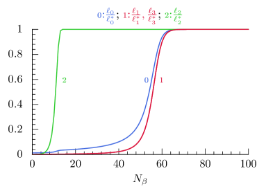
Figure 1: plot of $\frac{{\mbox{\boldmath$\ell$}}}{{\mbox{\boldmath$\ell$}}^{*}}$ as a function of the iteration step $N_{\beta}$ for $\lambda_{0}\equiv\alpha_{0}=-0.01$. The relevant coupling $\ell_{2}$ (curve number 2, in green, color online) reaches its fixed point first, after which the marginal coupling $\ell_{0}$ (number 0, blue) tends to its fixed value, closely followed by the irrelevant couplings $\ell_{1}$ and $\ell_{3}$ (number 1, both are drawn in red since they are almost equal).

We define $n_{j}(\lambda_{0})$ for $j=0,1,2,3$ as the step of the flow at which the right-discrete derivative of $\ell_{j}/\ell_{j}^{*}$ with respect to the step $N_{\beta}$ is largest. The reason for this definition is that, as $\lambda_{0}$ tends to $0$, the flow of $\ell_{j}$ tends to a step function, so that for each component $j$ the scale $n_{j}$ is a good measure of the number of iterations needed for that component to reach its fixed value. The Kondo temperature $\beta_{K}$ is defined as $2^{n_{0}(\lambda_{0})}$, and is the temperature at which the non-trivial fixed point is reached by all components. For small $\lambda_{0}$, we find that (see Fig.7), for $j=0,1,3$,

$$n_{j}(\lambda_{0})=c_{0}|\lambda_{0}|^{-1}+O(1),\quad c_{0}\approx 0.5$$ (58)

and (see Fig.8)

$$n_{2}(\lambda_{0})=c_{2}|\log_{2}|\lambda_{0}||+O(1),\quad c_{2}\approx 2.$$ (59)

(2) In addition to the previously mentioned fixed point ${\mbox{\boldmath$\ell$}}^{*}$, there are at least three extra fixed points, located at ${\mbox{\boldmath$\ell$}}_{0}^{*}{\buildrel def\over{=}}(0,0,0,0)$ and ${\mbox{\boldmath$\ell$}}_{\pm}^{*}{\buildrel def\over{=}}(0,0,\pm 1/3,0)$ (see Fig.2).

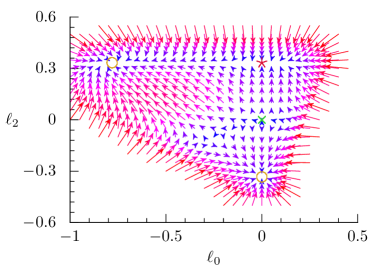
Figure 2: phase diagram of the flow projected on the $(\ell_{0},\ell_{2})$ plane, with initial conditions chosen in the plane that contains all four fixed points: ${\mbox{\boldmath$\ell$}}^{*}$ (which is linearly stable and represented by a yellow circle), ${\mbox{\boldmath$\ell$}}^{*}_{0}$ (which has one linearly unstable direction and one quadratically marginal and is represented by a green cross), ${\mbox{\boldmath$\ell$}}_{+}^{*}$ (which has one linearly stable direction and one quadratically marginal and is represented by a red star), and ${\mbox{\boldmath$\ell$}}_{-}^{*}$ (which is linearly stable, and is represented by a yellow circle).

When the running coupling constants are at ${\mbox{\boldmath$\ell$}}^{*}$, the susceptibility remains finite as $\beta\to\infty$ and positive, whereas when they are at ${\mbox{\boldmath$\ell$}}_{+}^{*}$, it grows linearly with $\beta$ (which is why ${\mbox{\boldmath$\ell$}}_{+}^{*}$ was called “trivial” in the introduction).

In addition, when $\lambda_{0}<0$ the flow escapes along the unstable direction towards the neighborhood of ${\mbox{\boldmath$\ell$}}^{*}_{+}$, which is reached after $n_{2}(\lambda_{0})$ steps, but since it is marginally unstable for $\lambda_{0}<0$, it flows away towards ${\mbox{\boldmath$\ell$}}^{*}$ after $n_{K}(\lambda_{0})$ steps. The susceptibility is therefore finite for $\lambda_{0}<0$ (see Fig.3 (which may be compared to the exact solution (AFL983, , Fig.3))).

If $\lambda_{0}>0$, then the flow approaches ${\mbox{\boldmath$\ell$}}^{*}_{+}$ from the $\lambda_{0}>0$ side, which is marginally stable, so the flow never leaves the vicinity of $\ell_{+}^{*}$ and the susceptibility diverges as $\beta\to\infty$.

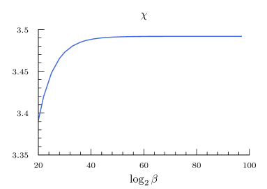
Figure 3: plot of $\chi(\beta,0)$ as a function of $\log_{2}\beta$ for $\lambda_{0}=-0.28$.

(3) We now discuss the flow at $h>0$ and address the question of continuity of the susceptibility in $h$ as $h\to 0$. If $\lambda_{0}<0$ and $\alpha_{5}=h\ll\beta_{K}^{-1}=2^{-n_{K}(\lambda_{0})}$, $\ell_{0}$ through $\ell_{3}$ first behave similarly to the $h=0$ case and tend to the same fixed point ${\mbox{\boldmath$\ell$}}^{*}$ and stay there until $\ell_{4}$ through $\ell_{8}$ become large enough, after which the flow tends to a fixed point in which $\ell_{2}=1/3$, $\ell_{5}=2$ and $\ell_{j}=0$ for $j\neq 2,5$ (see Fig.4).

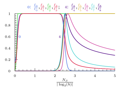
Figure 4: plot of $\frac{{\mbox{\boldmath$\ell$}}}{{\mbox{\boldmath$\ell$}}^{*}}$ as a function of the iteration step $N_{\beta}$ for $\lambda_{0}=-0.01$ and $h=2^{-40}$. Here $\ell_{0}^{*}$ through $\ell_{3}^{*}$ are the components of the non-trivial fixed point ${\mbox{\boldmath$\ell$}}^{*}$ and $\ell_{4}^{*}$ through $\ell_{8}^{*}$ are the values reached by $\ell_{4}$ through $\ell_{8}$ of largest absolute value. The flow behaves similarly to that at $h=0$ until $\ell_{4}$ through $\ell_{8}$ become large, at which point the couplings decay to 0, except for $\ell_{5}$ and $\ell_{2}$.

Setting the initial conditions for the flow as $\alpha_{j}=\alpha_{j}^{*}$ for $j=0,1,2,3$ and $\alpha_{5}=h$, we define $r_{j}(h)$ for $j=0,1,3$ and $j=4,5,6,7,8$ as the step of the flow at which the discrete derivative of $\ell_{j}/\ell_{j}^{*}$ is respectively smallest (that is most negative) and largest. Thus $r_{j}(h)$ measures when the flow leaves ${\mbox{\boldmath$\ell$}}^{*}$. We find that (see Fig.9) for small $h$,

$$r_{j}(h)=c_{r}\log_{2}h^{-1}+O(1),\quad c_{r}\approx 2.6.$$ (60)

Note that the previous picture only holds if $r_{j}(h)\gg\log_{2}(\beta_{K})$, that is $\beta_{K}h\ll 1$.

The susceptibility at $0<h\ll\beta_{K}^{-1}$ is continuous in $h$ as $h\to 0$ (see Fig.5). This, combined with the discussion in point (2) above, implies that the hierarchical Kondo model exhibits a Kondo effect.

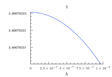
Figure 5: plot of $\chi(\beta,h)$ for $h\leq 10^{-6}$ at $\lambda_{0}=-0.28$ and $\beta=2^{20}$ (so that the largest value for $\beta h$ is $\sim 1$).

(4) In (Wi975, , Fig.17, p.836), there is a plot of $\frac{\beta_{K}}{\chi(\beta,0)}$ as a function of $\frac{\beta_{K}}{\beta}$. For the sake of comparison, we have reproduced it for the hierarchical Kondo model (see Fig.6).

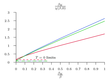
Figure 6: plot of $\frac{\beta_{K}}{\chi(\beta,0)}$ as a function of $\frac{\beta_{K}}{\beta}$ for various values of $\lambda_{0}$: $\lambda_{0}=-0.024$ (blue), $\lambda_{0}=-0.02412$ (green), $\lambda_{0}=-0.05$ (red). In Wi975 , $\lambda_{0}=-0.024$ and $-0.02412$. Note that the abscissa of the data points are $2^{-n}$ for $n\geq 0$, so that there are only $3$ points in the range $[0.25,1]$. The lines are drawn for visual aid.

Similarly to Wi975 , we find that $\frac{\beta_{K}}{\chi}$ seems to be affine as it approaches the Kondo temperature, although it is hard to tell for sure because of the scarcity of data points (by its very construction, the hierarchical Kondo model only admits inverse temperatures that are powers of 2 so the portion of Fig.6 that appears to be affine actually only contains three data points). However, we have found that such a diagram depends on $\lambda_{0}$: indeed, by sampling values of $|\lambda_{0}|$ down to $10^{-4}$, $\frac{\beta_{K}}{\chi(\beta,0)}$ has been found to tend to 0 faster than $(\log\beta_{K})^{-1.2}$ but slower than $(\log\beta_{K})^{-1.3}$. In order to get a more precise estimate on this exponent, one would need to consider $|\lambda_{0}|$ that are smaller than $10^{-4}$, which would give rise to numerical values larger than $10^{5000}$, and since the numbers used to perform the numerical computations are x86-extended precision floating point numbers, such values are too large.

7 Concluding remarks

(a) The hierarchical Kondo model defined in Sec.4 is a well defined statistical mechanics model, for which the partition function and correlation functions are unambiguously defined and finite as long as $\beta$ is finite. In addition, since the magnetic susceptibility of the impurity can be rewritten as a correlation function:

$$\chi(\beta,0)=\int_{0}^{\beta}dt\,{{\mbox{\boldmath$\langle$}}\,(\varphi^{+}(0){\mbox{\boldmath$\sigma$}}\varphi^{-}(0))(\varphi^{+}(t){\mbox{\boldmath$\sigma$}}\varphi^{-}(t))\,{\mbox{\boldmath$\rangle$}}}_{h=0},$$ (61)

$\chi(\beta,0)$ is a thermodynamical quantity of the model. (b) The qualitative behavior of the renormalization group flow is unchanged if all but the relevant and marginal running coupling constants (i.e. six constants out of nine) of the beta functions of Sec.5,6 are neglected (i.e. set to $0$ at every step of the iteration). In particular, we still find a Kondo effect. (c) In the hierarchical model defined in Sec.4, quantities other than the magnetic susceptibility of the impurity can be computed, although all observables must only involve fields localized at $x=0$. For instance, the response to a magnetic field acting on all sites of the fermionic chain as well as the impurity cannot be investigated in this model, since the sites of the chain with $x\neq 0$ are not accounted for.

(c.a) We have attempted to extend the definition of the hierarchical model to allow observables on the sites of the chain at $x\neq 0$ by paving the space-time plane with square boxes (instead of paving the time axis with intervals, see Sec.4), defining hierarchical fields for each quarter box and postulating a propagator between them by analogy with the non-hierarchical model. The magnetic susceptibility of the impurity is defined as the response to a magnetic field acting on every site of the chain and on the impurity, to which the susceptibility of the non-interacting chain is subtracted. We have found, iterating the flow numerically, that for such a model there is no Kondo effect, that is the impurity susceptibility diverges as $\beta$ when $\beta\to\infty$.

(c.b) A second approach has yielded better results, although it is not completely satisfactory. The idea is to incorporate the effect of the magnetic field $h$ acting on the fermionic chain into the propagator of the non-hierarchical model, after which the potential $V$ only depends on the site at $x=0$, so that the hierarchical model can be defined in the same way as in Sec.4 but with an $h$-dependent propagator. In this model, we have found that there is a Kondo effect.

Appendix A Comparison with the original Kondo model

If the partition function for the original Kondo model in presence of a magnetic field $h$ acting only on the impurity site and at finite $L$ is denoted by $Z^{0}_{K}(\beta,\lambda_{0},h)$ and the partition function for the model Eq.(1) with the same field $h$ is denoted by $Z_{K}(\beta,\lambda_{0},h)$, then

$$Z_{K}(\beta,\lambda_{0},h)=Z^{0}_{K}(\beta,\lambda_{0},h)+Z^{0}_{K}(\beta,0,0)$$ (62)

so that by defining

$$\kappa\,{\buildrel def\over{=}}\,1+\frac{Z^{0}_{K}(\beta,0,0)}{Z^{0}_{K}(\beta,\lambda_{0},h)}$$ (63)

we get

$$m_{K}(\beta,\lambda_{0},h) = \frac{1}{\kappa}{m^{0}_{K}(\beta,\lambda_{0},h)},$$

$$m^{0}_{K}(\beta,\lambda_{0},h) = \kappa\,m_{K}(\beta,\lambda_{0},h)$$ (64)

$$\chi_{K}(\beta,\lambda_{0},h) = \frac{1}{\kappa}\,{\chi_{K}^{0}(\beta,\lambda_{0},h)}+\frac{\kappa-1}{\kappa}\,\beta\,m^{0}_{K}(\beta,\lambda_{0},h)^{2}$$

$$\chi_{K}^{0}(\beta,\lambda_{0},h) = \kappa\,\chi_{K}(\beta,\lambda_{0},h)-(\kappa-1)\beta m_{K}(\beta,\lambda_{0},h)^{2}.$$

In addition $1\leq\kappa\leq 2$: indeed the first inequality is trivial and the second follows from the variational principle (see (Ru969, , theorem 7.4.1, p.188)):

$$\log Z^{0}_{K}(\beta,\lambda_{0},h) = \max_{\mu}(s(\mu)-\mu(H_{0}+V))$$ (65)

$$\geq s(\mu_{0})-\mu_{0}(H_{0})+\mu_{0}(V)=s(\mu_{0})-\mu_{0}(H_{0})=\log Z^{0}_{K}(\beta,0,0)$$

where $s(\mu)$ is the entropy of the state $\mu$, and in which we used

$$\mu_{0}(V)={\rm Tr}\,(e^{-\beta H_{0}}\,V)/Z_{K}(\beta,0,0)=0.$$ (66)

Therefore, for $\beta h^{2}\ll 1$ (which implies that if there is a Kondo effect then $\beta m_{K}^{2}\ll 1$), the model Eq.(1) exhibits a Kondo effect if and only if the original Kondo model does, therefore, for the purposes of this paper, both models are equivalent.

Appendix B Some identities.

In this appendix, we state three relations used to compute the flow equation Eq.(44), which follow from a patient algebraic meditation:

$${{\mbox{\boldmath$\langle$}}\,A_{1}^{j_{1}}A_{2}^{j_{2}}\,{\mbox{\boldmath$\rangle$}}} = \delta_{j_{1},j_{2}}\Big{(}2+\frac{1}{3}{\bf a}^{2}\Big{)}-2\,a^{j_{1},j_{2}}\delta_{j_{1}\neq j_{2}}\,s_{t_{2},t_{1}}$$

$${{\mbox{\boldmath$\langle$}}\,A^{j_{1}}_{1}A^{j_{2}}_{1}A^{j_{3}}_{2}\,{\mbox{\boldmath$\rangle$}}} \equiv 2\,a^{j_{3}}\,\delta_{j_{1},j_{2}}$$ (67)

$${{\mbox{\boldmath$\langle$}}\,A_{1}^{j_{1}}A_{1}^{j_{2}}A_{2}^{j_{3}}A_{2}^{j_{4}}\,{\mbox{\boldmath$\rangle$}}} = 4\delta_{j_{1},j_{2}}\delta_{j_{3},j_{4}}$$

where the lower case ${\bf a}$ denote ${{\mbox{\boldmath$\langle$}}\,{\bf A}_{1}\,{\mbox{\boldmath$\rangle$}}}\equiv{{\mbox{\boldmath$\langle$}}\,{\bf A}_{2}\,{\mbox{\boldmath$\rangle$}}}$ and $a^{j_{1},j_{2}}={{\mbox{\boldmath$\langle$}}\,\psi^{+}_{1}\sigma^{j_{1}}\sigma^{j_{2}}\psi^{-}_{1}\,{\mbox{\boldmath$\rangle$}}}={{\mbox{\boldmath$\langle$}}\,\psi^{+}_{2}\sigma^{j_{1}}\sigma^{j_{2}}\psi^{-}_{2}\,{\mbox{\boldmath$\rangle$}}}$.

Appendix C Complete beta function

The beta function for the flow described in Sec.6 is

$$\ell_{0}^{[m-1]} = \frac{1}{C^{[m]}}(\ell_{0}-2\ell_{0}\ell_{6}+18\ell_{0}\ell_{3}+3\ell_{0}\ell_{2}+3\ell_{0}\ell_{1}-2\ell_{0}^{2})$$

$$\ell_{1}^{[m-1]} = \frac{1}{C^{[m]}}(\frac{1}{2}\ell_{1}+9\ell_{2}\ell_{3}+\frac{3}{2}\ell_{8}^{2}+\frac{1}{12}\ell_{6}^{2}+\frac{1}{2}\ell_{5}\ell_{7}+\frac{1}{24}\ell_{4}^{2}+\frac{1}{6}\ell_{0}\ell_{6}+\frac{1}{4}\ell_{0}^{2})$$

$$\ell_{2}^{[m-1]} = \frac{1}{C^{[m]}}(2\ell_{2}+36\ell_{1}\ell_{3}+\ell_{0}^{2}+6\ell_{7}^{2}+\frac{1}{3}\ell_{6}^{2}+\frac{1}{6}\ell_{5}^{2}+2\ell_{4}\ell_{8}+\frac{2}{3}\ell_{0}\ell_{6})$$ (68)

$$\ell_{3}^{[m-1]} = \frac{1}{C^{[m]}}(\frac{1}{2}\ell_{3}+\frac{1}{4}\ell_{1}\ell_{2}+\frac{1}{24}\ell_{0}^{2}+\frac{1}{36}\ell_{0}\ell_{6}+\frac{1}{72}\ell_{6}^{2}+\frac{1}{12}\ell_{5}\ell_{7}+\frac{1}{12}\ell_{4}\ell_{8})$$

$$\ell_{4}^{[m-1]} = \frac{1}{C^{[m]}}(\ell_{4}+6\ell_{6}\ell_{7}+\ell_{5}\ell_{6}+108\ell_{3}\ell_{8}+18\ell_{2}\ell_{8}+3\ell_{1}\ell_{4}+6\ell_{0}\ell_{7}+\ell_{0}\ell_{5})$$

$$\ell_{5}^{[m-1]} = \frac{1}{C^{[m]}}(2\ell_{5}+12\ell_{6}\ell_{8}+2\ell_{4}\ell_{6}+216\ell_{3}\ell_{7}+6\ell_{2}\ell_{5}+36\ell_{1}\ell_{7}+12\ell_{0}\ell_{8}+2\ell_{0}\ell_{4})$$

$$\ell_{6}^{[m-1]} = \frac{1}{C^{[m]}}(\ell_{6}+18\ell_{7}\ell_{8}+3\ell_{5}\ell_{8}+3\ell_{4}\ell_{7}+\frac{1}{2}\ell_{4}\ell_{5}+18\ell_{3}\ell_{6}+3\ell_{2}\ell_{6}+3\ell_{1}\ell_{6}$$

$$\hskip 25.0pt+2\ell_{0}\ell_{6})$$

$$\ell_{7}^{[m-1]} = \frac{1}{C^{[m]}}(\frac{1}{2}\ell_{7}+\frac{1}{2}\ell_{6}\ell_{8}+\frac{1}{12}\ell_{4}\ell_{6}+\frac{3}{2}\ell_{3}\ell_{5}+\frac{3}{2}\ell_{2}\ell_{7}+\frac{1}{4}\ell_{1}\ell_{5}+\frac{1}{2}\ell_{0}\ell_{8}$$

$$\hskip 25.0pt+\frac{1}{12}\ell_{0}\ell_{4})$$

$$\ell_{8}^{[m-1]} = \frac{1}{C^{[m]}}(\ell_{8}+\ell_{6}\ell_{7}+\frac{1}{6}\ell_{5}\ell_{6}+3\ell_{3}\ell_{4}+\frac{1}{2}\ell_{2}\ell_{4}+3\ell_{1}\ell_{8}+\ell_{0}\ell_{7}+\frac{1}{6}\ell_{0}\ell_{5})$$

$$C^{[m]} = 1+2\ell_{0}^{2}+(\ell_{0}+\ell_{6})^{2}+9\ell_{1}^{2}+9\ell_{2}^{2}+324\ell_{3}^{2}+\frac{1}{2}\ell_{4}^{2}+\frac{1}{2}\ell_{5}^{2}+18\ell_{7}^{2}+18\ell_{8}^{2}$$

in which we dropped the ^[m] exponent on the right side. By considering the linearized flow equation (around $\ell_{j}=0$), we find that $\ell_{0},\ell_{4},\ell_{6},\ell_{8}$ are marginal, $\ell_{2},\ell_{5}$ relevant and $\ell_{1},\ell_{3},\ell_{7}$ irrelevant. The consequent linear flow is very different from the full flow discussed in Sec.6.

The vector $\ell$ is related to $\alpha$ and via the following map:

$$\ell_{0} = \alpha_{0},\quad\ell_{1}=\alpha_{1}+\frac{1}{12}\alpha_{4}^{2},\quad\ell_{2}=\alpha_{2}+\frac{1}{12}\alpha_{5}^{2}$$

$$\ell_{3} = \alpha_{3}+\frac{1}{12}\alpha_{0}^{2}+\frac{1}{18}\alpha_{0}\alpha_{6}+\frac{1}{2}\alpha_{1}\alpha_{2}+\frac{1}{6}\alpha_{4}\alpha_{8}+\frac{1}{6}\alpha_{5}\alpha_{7}+\frac{1}{36}\alpha_{6}^{2}$$ (69)

$$+\frac{1}{36}\alpha_{0}\alpha_{4}\alpha_{5}+\frac{1}{24}\alpha_{1}\alpha_{5}^{2}+\frac{1}{24}\alpha_{2}\alpha_{4}^{2}+\frac{1}{36}\alpha_{4}\alpha_{5}\alpha_{6}+\frac{1}{288}\alpha_{4}^{2}\alpha_{5}^{2}$$

$$\ell_{4} = \alpha_{4},\quad\ell_{5}=\alpha_{5},\quad\ell_{6}=\alpha_{6}+\frac{1}{2}\alpha_{4}\alpha_{5}$$

$$\ell_{7} = \alpha_{7}+\frac{1}{6}\alpha_{0}\alpha_{4}+\frac{1}{2}\alpha_{1}\alpha_{5}+\frac{1}{6}\alpha_{4}\alpha_{6}+\frac{1}{24}\alpha_{4}^{2}\alpha_{5}$$

$$\ell_{8} = \alpha_{8}+\frac{1}{6}\alpha_{0}\alpha_{5}+\frac{1}{2}\alpha_{2}\alpha_{4}+\frac{1}{6}\alpha_{5}\alpha_{6}+\frac{1}{24}\alpha_{4}\alpha_{5}^{2}.$$

Appendix D The algebra of the operators $O_{n,\pm}$.

Lemma 1

Given $\eta\in\{-,+\}$, $m\leq 0$ and $\Delta\in\mathcal{Q}_{m}$, the span of the operators $\{O_{n,\eta}^{[\leq m]}(\Delta)\}_{n\in\{0,1,2,3\}}$ defined in Eq.(37) is an algebra, that is all linear combinations of products of $O_{n,\eta}^{[\leq m]}(\Delta)$’s is itself a linear combination of $O_{n,\eta}^{[\leq m]}(\Delta)$’s.
The same result holds for the span of the operators $\{O_{n,\eta}^{[\leq m]}(\Delta)\}_{n\in\{0,\cdots,8\}}$ defined in Eq.(53).

Proof: The only non-trivial part of this proof is to show that the product of two $O_{n,\eta}$’s is a linear combination of $O_{n,\eta}$’s.

Due to the anti-commutation of Grassmann variables, any linear combination of $\psi_{\alpha}^{[\leq m]\pm}$ and $\varphi_{\alpha}^{[\leq m]\pm}$ squares to 0. Therefore, a straightforward computation shows that $\forall(i,j)\in\{1,2,3\}^{2}$,

$$A^{i}_{\eta}A^{j}_{\eta}=2\delta_{i,j}\psi^{+}_{\uparrow}\psi^{+}_{\downarrow}\psi^{-}_{\uparrow}\psi^{-}_{\downarrow},\quad B^{i}_{\eta}B^{j}_{\eta}=2\delta_{i,j}\varphi^{+}_{\uparrow}\varphi^{+}_{\downarrow}\varphi^{-}_{\uparrow}\varphi^{-}_{\downarrow}$$ (70)

where the labels ^[≤m] and $(\Delta)$ are dropped to alleviate the notation. In particular, this implies that any product of three $A^{i}_{\eta}$ for $i\in\{1,2,3\}$ vanishes (because the product of the right side of the first of Eq.(70) and any Grassmann field $\psi_{\alpha}^{\pm}$ vanishes) and similarly for the product of three $B^{i}_{\eta}$.

Using Eq.(70), we prove that $\mathrm{span}\{O_{n,\eta}^{[\leq m]}(\Delta)\}_{n\in\{0,1,2,3\}}$ is an algebra. For all $n\in\{0,1,2,3\}$, $p\in\{1,2,3\}$, $l\in\{1,2\}$,

$$O_{p}^{2}=0,\quad O_{3}O_{n}=0,\quad O_{l}O_{0}=0,\quad O_{0}^{2}=\frac{1}{6}O_{3},\quad O_{1}O_{2}=\frac{1}{2}O_{3}$$ (71)

(here the ^[≤m], $(\Delta)$ and _η are dropped). This concludes the proof of the first claim.

Next we prove that $\mathrm{span}\{O_{n,\eta}^{[\leq m]}(\Delta)\}_{n\in\{0,\cdots,8\}}$ is an algebra. In addition to Eq.(71), we have, for all $p\in\{0,\cdots,8\}$,

$$O_{0}O_{4}=\frac{1}{6}O_{7},\quad O_{0}O_{5}=\frac{1}{6}O_{8},\quad O_{0}O_{6}=\frac{1}{18}O_{3},\quad O_{0}O_{7}=O_{0}O_{8}=0,\quad O_{1}O_{5}=\frac{1}{2}O_{7},$$

$$O_{1}O_{4}=O_{1}O_{6}=O_{1}O_{7}=O_{1}O_{8}=0,\quad O_{2}O_{4}=\frac{1}{2}O_{8},\quad O_{2}O_{5}=O_{2}O_{6}=O_{2}O_{7}=O_{2}O_{8}=0,$$

$$O_{3}O_{p}=0,\quad O_{4}^{2}=\frac{1}{6}O_{1},\quad O_{4}O_{5}=\frac{1}{2}O_{6},\quad O_{4}O_{8}=\frac{1}{6}O_{3},\quad O_{4}O_{7}=0,\quad O_{5}^{2}=\frac{1}{6}O_{2},$$ (72)

$$O_{5}O_{7}=\frac{1}{6}O_{3},\quad O_{5}O_{8}=0,\quad O_{6}^{2}=\frac{1}{18}O_{3},\quad O_{6}O_{7}=O_{6}O_{8}=0,\quad O_{7}^{2}=O_{8}^{2}=O_{7}O_{8}=0.$$

This concludes the proof of the lemma.

Appendix E Fixed points at $h=0$

We first compute the fixed points of Eq.(44) for $\ell_{2}\geq 0$. It follows from Eq.(44) that if $\ell$ is a fixed point, then $\ell_{1}=6\ell_{3}$, which implies

$$(1-3\ell_{2})\left(\ell_{2}(1+3\ell_{2})+6\ell_{1}^{2}+\ell_{0}^{2}\right)=0.$$ (73)

If $\ell_{2}\geq 0$, Eq.(73) implies that either $\ell_{2}=\ell_{1}=\ell_{0}=0$ or $\ell_{2}=\frac{1}{3}$. In the latter case, either $\ell_{0}=\ell_{1}=0$ or $\ell_{0}\not=0$ and Eq.(44) becomes

$$\left\{\begin{array}[]{l}3\ell_{0}^{2}+2\ell_{0}+6\ell_{1}(3\ell_{1}-1)=0\\[8.5359pt] \ell_{1}(1+18\ell_{1}^{2})+\ell_{0}^{2}(3\ell_{1}-\frac{1}{4})=0.\end{array}\right.$$ (74)

In particular, $\ell_{1}(1-12\ell_{1})>0$, so that

$$\ell_{0}=\pm 2\sqrt{\frac{\ell_{1}(1+18\ell_{1}^{2})}{1-12\ell_{1}}}$$ (75)

which we inject into Eq.(74) to find that $\ell_{0}<0$ and

$$1-\frac{35}{4}(3\ell_{1})+\frac{27}{2}(3\ell_{1})^{2}-\frac{19}{4}(3\ell_{1})^{3}+107(3\ell_{1})^{4}=0.$$ (76)

Finally, we notice that $\frac{1}{12}$ is a solution of Eq.(76), which implies that

$$4-19(3\ell_{1})-22(3\ell_{1})^{2}-107(3\ell_{1})^{3}$$ (77)

which has a unique real solution. Finally, we find that if $\ell_{1}$ satisfies Eq.(77), then

$$2\sqrt{\frac{\ell_{1}(1+18\ell_{1}^{2})}{1-12\ell_{1}}}=3\ell_{1}\frac{1+15\ell_{1}}{1-12\ell_{1}}.$$ (78)

We have therefore shown that, if $\ell_{2}\geq 0$, then Eq.(44) has three fixed points:

$${\mbox{\boldmath$\ell$}}_{0}^{*}:=(0,0,0,0),\quad{\mbox{\boldmath$\ell$}}_{+}^{*}:=\left(0,0,\frac{1}{3},0\right),$$

$${\mbox{\boldmath$\ell$}}^{*}:=\left(-x_{0}\frac{1+5x_{0}}{1-4x_{0}},\frac{x_{0}}{3},\frac{1}{3},\frac{x_{0}}{18}\right).$$ (79)

In addition, it follows from Eq.(44) and Eq.(42) that, if $\lambda_{0}<0$, then (recall that $\alpha_{0}^{[0]}=\lambda_{0}$ and $\alpha_{i}^{[0]}=0$, $i=1,2,3$)

$$\ell_{0}^{[m]}<0,\quad 0\leq\ell_{2}^{[m]}<\frac{1}{3},\quad 0\leq\ell_{1}^{[m]}<6\ell_{3}^{[m]}<\frac{1}{12}$$ (80)

for all $m\leq 0$, which implies that the set $\{{\mbox{\boldmath$\ell$}}\ |\ \ell_{0}<0,\ \ell_{2}\geq 0,\ \ell_{1}\geq 0,\ \ell_{3}\geq 0\}$ is stable under the flow. In addition, if $\ell_{0}^{[m]}>-\frac{2}{3}$, then $\ell_{0}^{[m-1]}<\ell_{0}^{[m]}$, so that the flow cannot converge to ${\mbox{\boldmath$\ell$}}_{0}^{*}$ or ${\mbox{\boldmath$\ell$}}_{+}^{*}$. Therefore if the flow converges, then it converges to ${\mbox{\boldmath$\ell$}}^{*}$.

We now study the reduced flow Eq.(48), and prove that starting from $-2/3<\ell^{[0]}_{0}<0$, $\ell^{[0]}_{2}=0$, the flow converges to $f^{*}$. It follows from Eq.(48) that $\ell^{[m]}_{0}<0$, $\ell^{[m]}_{2}>0$ for all $m<0$, so that if Eq.(48) converges to a fixed point, then it must converge to $f^{*}$. In addition, by a straightforward induction, one finds that $\ell_{2}^{[m-1]}>\ell_{2}^{[m]}$ if $\ell_{2}^{[m]}<\frac{1}{3}$. Furthermore, $(2\ell_{2}^{[m]}+(\ell_{0}^{[m]})^{2})\leq\frac{1}{3}C^{[m]}$, which implies that $\ell_{2}^{[m]}\leq\frac{1}{3}$. Therefore $\ell_{2}^{[m]}$ converges as $m\to-\infty$. In addition, $\ell_{0}^{[m-1]}<\ell_{0}^{[m]}$ if $\ell_{0}^{[m]}>-\frac{2}{3}$, and $\ell_{0}^{[m]}>-\frac{1}{3}-\ell_{2}^{[m]}\geq-\frac{2}{3}$, so that $\ell_{0}^{[m]}$ converges as well as $m\to-\infty$. The flow therefore tends to $f^{*}$.

Finally, we prove that starting from $\ell^{[0]}_{0}>0,\ell^{[0]}_{2}=0$, the flow converges to $f_{+}$. Similarly to the anti-ferromagnetic case, $\ell^{[m]}_{2}>0$ for all $m<0$, $\ell_{2}^{[m]}\leq\frac{1}{3}$ and $\ell_{2}^{[m-1]}>\ell_{2}^{[m]}$. In addition, by a simple induction, if $\lambda_{0}<1$, then $\ell_{0}^{[m]}>0$ and $\ell_{0}^{[m]}+\frac{1}{3}-\ell_{2}^{[m]}$ is strictly decreasing and positive. In conclusion, $\ell_{0}^{[m]}$ and $\ell_{2}^{[m]}$ converge to $f_{+}$.

Appendix F Asymptotic behavior of $n_{j}(\lambda_{0})$ and $r_{j}(h)$

In this appendix, we show plots to support the claims on the asymptotic behavior of $n_{j}(\lambda_{0})$ (see Eq.(58), Fig.7 and Eq.(59), Fig.8) and $r_{j}(h)$ (see Eq.(60), Fig.9). The plots below have error bars which are due to the fact that $n_{j}(\lambda_{0})$ and $r_{j}(h)$ are integers, so their value could be off by $\pm 1$.

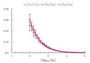
Figure 7: plot of $n_{j}(\lambda_{0})|\lambda_{0}|$ for $j=0$ (blue, color online) and $j=1,3$ (red) as a function of $|\log_{10}|\lambda_{0}||$. This plot confirms Eq.(58).

Figure 8: plot of $n_{2}(\lambda_{0})|\log_{2}|\lambda_{0}||^{-1}$ as a function of $|\log_{10}|\lambda_{0}||$. This plot confirms Eq.(59).

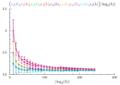
Figure 9: plot of $r_{j}(h)|\log_{2}(h)||$ as a function of $|\log_{2}(h)|$. This plot confirms Eq.(60).

Appendix G Kondo effect, XY-model, free fermions

In ABGM971 , given $\nu\in[1,\ldots,L]$, the Hamiltonian ${\cal H}_{h}={\cal H}_{0}{-h}\,\sigma_{\nu}^{z}$, with

$${\cal H}_{0}={-\frac{1}{4}}\sum_{n=1}^{L}(\sigma^{x}_{n}\sigma^{x}_{n+1}+\sigma^{y}_{n}\sigma^{y}_{n+1}).$$ (81)

has been considered with suitable boundary conditions (see App.H), under which $H_{0}$ and ${\sigma^{z}_{0}}+1$ are unitarily equivalent to $\sum_{q}{(-\cos q)}\,a^{+}_{q}a^{-}_{q}$ and, respectively, to $\frac{2}{L}\sum_{q,q^{\prime}}a^{+}_{q}a^{-}_{q^{\prime}}e^{i\nu(q-q^{\prime})}$ in which $a^{\pm}_{q}$ are fermionic creation and annihilation operators and the sums run over $q$’s that are such that $e^{iqL}=-1$. It has been shown, ABGM971 , that, by defining

$$F_{L}(\zeta) = 1+\frac{2h}{L}\sum_{q}\frac{1}{\zeta+\cos q}$$

$$F(z) = \lim_{L\to\infty}F_{L}(z)=1+\frac{2\,h}{\pi}\,\int_{0}^{\pi}\frac{dq}{(z+\cos q)}$$ (82)

the partition function is equal to $Z_{L}^{0}\zeta_{L}$ in which $Z_{L}^{0}$ is the partition function at $h=0$ and is extensive (i.e. of $O(e^{constL})$) and (see App.H, Eq.(102))

$$\log{\zeta_{L}(\beta,h)}=-\beta h+\frac{1}{2\pi i}\oint_{C}\log(1+{e^{-\beta z}})\Big{[}\frac{\partial_{z}F_{L}(z)}{F_{L}(z)}\Big{]}\,dz$$ (83)

where the contour $C$ is a closed curve which contains the zeros of $F_{L}(\zeta)$ (e.g. , for $L\to\infty$, a curve around the real interval $[-1,\sqrt{1+4h^{2}}]$ if $h<0$ and $[-\sqrt{1+4h^{2}},1]$ if $h>0$) but not around those of $1+e^{-\beta\zeta}$ (which are on the imaginary axis and away from $0$ by at least $\frac{\pi}{\beta}$). In addition, it follows from a straightforward computation that $(F(z)-1)/h$ is equal to the analytical continuation of $2(z^{2}-1)^{-\frac{1}{2}}$ from $(1,\infty)$ to $C\setminus[-1,1]$.

At fixed $\beta<\infty$ the partition function $\zeta_{L}(\beta,h)$ has a non extensive limit $\zeta(\beta,h)$ as $L\to\infty$; the $\zeta(\beta,h)$ and the susceptibility and magnetization values $m(\beta,h)$ and $\chi(\beta,h)$, are given in the thermodynamic limit by

$$\log\zeta(\beta,h) = -\beta h{+\frac{\beta}{2\pi i}}\oint_{C}\frac{dz}{1+{e^{\beta z}}}\log(1{+}\frac{2h}{(z^{2}-1)^{\frac{1}{2}}})$$

$$m(\beta,h) = -1+\frac{1}{\pi i}\oint_{C}\frac{1}{1+{e^{\beta z}}}\frac{dz}{(z^{2}-1)^{\frac{1}{2}}{+2h}}$$ (84)

$$\chi(\beta,h) = -\frac{2}{\pi i}\oint_{C}\frac{1}{1+{e^{\beta z}}}\frac{dz}{((z^{2}-1)^{\frac{1}{2}}{+2h})^{2}}$$

so that $\chi(\beta,0)=\frac{2\sinh(\beta)}{(1+\cosh(\beta))}$ and, in the $\beta\to\infty$ limit,

$$m(\infty,h)=\frac{2h}{\sqrt{1+4h^{2}}},\quad\chi(\infty,h)=\frac{2}{(1+4h^{2})^{3/2}}$$ (85)

both of which are finite. Adding an impurity at $0$, with spin operators ${\mbox{\boldmath$\tau$}}_{0}$, the Hamiltonian

$$H_{\lambda}=H_{0}{-h}(\sigma^{z}_{0}+\tau^{z}_{0}){-\lambda}\sigma^{z}_{0}\tau^{z}_{0}$$ (86)

is obtained. Does it exhibit a Kondo effect?

Since ${\mbox{\boldmath$\tau$}}_{0}$ commutes with the ${\mbox{\boldmath$\sigma$}}_{n}$ and, hence, with $H_{0}$, the average magnetization and susceptibility, $m^{int}(\beta,h,\lambda)$ and $\chi^{int}(\beta,h,\lambda)$, responding to a field $h$ acting only on the site $0$, can be expressed in terms of the functions $\zeta(\beta,h)$ and its derivatives $\zeta^{\prime}(\beta,h)$ and $\zeta^{\prime\prime}(\beta,h)$. By using the fact that $\zeta(\beta,h)$ and $\zeta^{\prime\prime}(\beta,h)$ are even in $h$, while $\zeta^{\prime}(\beta,h)$ is odd, we get:

$$\chi^{int}(\beta,0) = \beta^{-1}\partial^{2}_{h}\log{\rm Tr}\,\sum_{\tau=\pm 1}\Big{(}e^{-\beta H_{0}+\beta\lambda\sigma^{z}\tau+\beta h(\sigma^{z}+\tau)}\Big{)}\Big{|}_{h=0}$$

$${\buildrel def\over{=}} \beta^{-1}\partial^{2}_{h}\log Z^{int}(\beta,h,\lambda)\Big{|}_{h=0}$$

$$= \beta^{-1}\Big{[}\sum_{\tau}\frac{\zeta^{\prime\prime}+\zeta^{\prime}\beta\tau+(\zeta^{\prime}+\beta\tau\zeta)\beta\tau}{Z^{int}}-\Big{(}\sum_{\tau}\frac{(\zeta^{\prime}+\beta\tau\zeta)}{Z^{int}}\Big{)}^{2}\Big{]}_{h=0}$$

$$= \chi(\beta,|\lambda|)+\beta(m(\beta,|\lambda|)+1)^{2}\,\vtop{\halign{#\cr\rightarrowfill\crcr\kern-1.0pt\nointerlineskip\cr\hskip 3.0pt${\scriptstyle\beta\to\infty}$\hskip 3.0pt\crcr}}\,+\infty$$ (90)

Since $\chi^{int}(\beta,0)$ is even in $\lambda$, it diverges for $\beta\to\infty$ independently of the sign of $\lambda$, while $\chi(\beta,0)$ is finite. Hence, the model yields Pauli’s paramagnetism, without a Kondo effect.

Remarks: (1) Finally an analysis essentially identical to the above can be performed to study the model in Eq.(1) without impurity (and with or without spin) to check that the magnetic susceptibility to a field $h$ acting only at a single site is finite: the result is the same as that of the XY model above: the single site susceptibility is finite and, up to a factor $2$, given by the same formula $\chi(\beta,0)=\frac{4\sinh\beta}{1+\cosh\beta}$.

(2) The latter result makes clear both the essential roles for the Kondo effect of the spin and of the noncommutativity of the impurity spin components.

Appendix H Some details on App.G

The definition of $H_{h}$ has to be supplemented by a boundary condition to give a meaning to ${\mbox{\boldmath$\sigma$}}_{L+1}$. If $\sigma^{\pm}_{n}=(\sigma^{x}\pm i\sigma^{y}_{n})/2$ define ${\cal N}_{<n}$ as $\sum_{i<n}\sigma^{+}_{i}\sigma^{-}_{i}=\sum_{i<n}{\cal N}_{i}$ and ${\cal N}={\cal N}_{\leq L}$. Then set as boundary condition

$$\sigma_{L+1}^{\pm}{\buildrel def\over{=}}-(-1)^{\cal N}\sigma^{\pm}_{1}$$ (91)

(parity-antiperiodic b.c.) so that $H_{h}$ becomes

$$H_{h} = -h(2\sigma^{+}_{\nu}\sigma^{-}_{\nu}-1)-\frac{1}{2}\sum_{n=1}^{L-1}(\sigma^{+}_{n}(-1)^{{\cal N}_{n}}\sigma^{-}_{n+1}+\sigma^{-}_{n}(-1)^{{\cal N}_{n}}\sigma^{+}_{n+1})$$

$$-\frac{1}{2}(\,\sigma^{+}_{L}(-1)^{{\cal N}_{L}}(-\sigma^{-}_{1})+\sigma^{-}_{L}(-1)^{{\cal N}_{L}}(-\sigma^{+}_{1})\,).$$

Introducing the Pauli-Jordan transformation

$$a^{\pm}_{n}=(-1)^{{\cal N}_{<n}}\sigma^{\pm}_{n},\qquad a^{\pm}_{L+1}=-a^{\pm}_{1}.$$ (93)

In these variables

$$H_{h}={-h(2a^{+}_{\nu}a^{-}_{\nu}-1)-\frac{1}{2}}\sum_{n=1}^{L-1}(a^{+}_{n}a^{-}_{n+1}-a^{-}_{n}a^{+}_{n+1})$$ (94)

Assume $L=$even and let $I{\buildrel def\over{=}}\{q|q=\pm\frac{(2n+1)\pi}{L},\,n=0,1,\ldots,\frac{L}{2}-1\}$; then

$$H_{h} = \sum_{q}{(-\cos q)}\,A^{+}_{q}A^{-}_{q}-\frac{h}{L}\sum_{q,q^{\prime}}(2A^{+}_{q}A^{-}_{q^{\prime}}e^{i(q-q^{\prime})\nu}-1)$$ (95)

$$A^{\pm}_{q} {\buildrel def\over{=}} \frac{1}{\sqrt{L}}\sum_{n=1}^{L}e^{\pm inq}a^{\pm}_{n},\qquad e^{iLq}=-1,\quad q\in I$$

In diagonal form let $U_{jq}$ be a suitable unitary matrix such that

$$H_{h}=\sum_{j}\lambda_{j}\alpha^{+}_{j}\alpha^{-}_{j},\qquad{\rm if}\ \alpha^{+}_{j}=\sum_{q}U_{jq}A^{+}_{q}$$ (96)

Then $\lambda_{j}$ must satisfy

$$\Big{(}-\sum_{q}\cos qA^{+}_{q}A^{-}_{q}-\frac{2h}{L}\sum_{q,q^{\prime}}A^{+}_{q}A^{-}_{q^{\prime}}e^{i(q-q^{\prime})\nu}\Big{)}\sum_{q^{\prime\prime}}U_{jq^{\prime\prime}}A^{+}_{q^{\prime\prime}}{{\mbox{\boldmath$|$}}0{\mbox{\boldmath$\rangle$}}}=\lambda_{j}\sum_{q^{\prime\prime}}U_{jq^{\prime\prime}}A^{+}_{q^{\prime\prime}}{{\mbox{\boldmath$|$}}0{\mbox{\boldmath$\rangle$}}}$$ (97)

$${\rm hence}\qquad (\lambda_{j}+\cos q)U_{jq}e^{-iq\nu}=-\frac{2h}{L}\sum_{q^{\prime\prime}}e^{-iq^{\prime\prime}\nu}U_{jq^{\prime\prime}},$$

$\forall q\in I$, where we used the fact that $A^{-}_{p}A^{+}_{q}{{\mbox{\boldmath$|$}}0{\mbox{\boldmath$\rangle$}}}=\delta_{p,q}{{\mbox{\boldmath$|$}}0{\mbox{\boldmath$\rangle$}}}$. We consider the two cases $\lambda_{j}\neq-\cos q$ for all $q\in I$ or $\lambda_{j}=-\cos q_{0}$ for some $q_{0}\in I$.

In the first case:

$$U_{jq}=\frac{e^{iq\nu}}{N(\lambda_{j})}\frac{1}{\lambda_{j}+\cos q},\quad{\rm provided}\quad F_{L}(\lambda_{j}){\buildrel def\over{=}}1+\frac{2h}{L}\sum_{q}\frac{1}{\lambda_{j}+\cos q}=0,$$ (98)

where $N(\lambda_{j})$ is set in such a way that $U$ is unitary, or, in the second case,

$$\lambda_{j}=-\cos q_{0},\quad U_{jq}=\frac{e^{iq\nu}}{\sqrt{2}}(\delta_{q,q_{0}}-\delta_{q,-q_{0}}),\ \ {\rm so\ that}\sum_{q^{\prime\prime}}e^{-iq^{\prime\prime}\nu}U_{jq^{\prime\prime}}=0.$$ (99)

Since $-\cos q$ takes $\frac{1}{2}L$ values and the equation $F_{L}(\lambda)=0$ has $\frac{L}{2}$ solutions, the spectrum of $H_{h}$ is completely determined and given by the $2^{L}$ eigenvalues

$$\lambda({\bf n})=\sum_{j}n_{j}\lambda_{j},\qquad{\bf n}=(n_{1},\ldots,n_{L}),\ n_{j}=0,1$$ (100)

and the partition function is

$$\log Z_{L}(\beta,h)=\sum_{q>0}\log(1+e^{\beta\cos q})+\sum_{j}\log(1+{e^{-\beta\lambda_{j}}})=\frac{1}{2}\log Z^{0}_{L}(\beta)+\sum_{j\in I}\log(1+{e^{-\beta\lambda_{j}}}).$$ (101)

On the other hand, since the function $F^{\prime}_{L}(z)/F_{L}(z)$ has $L/2$ poles with residue $+1$ (those corresponding to the zeros of $F_{L}(z)$) and $L/2$ poles with residue $-1$ (those corresponding to the poles of $F_{L}(z)$), the contour integral in the r.h.s. of Eq.(83) is equal to

$$\sum_{j}\log(1+e^{-\beta\lambda_{j}})-\sum_{q>0}\log(1+e^{\beta\cos q})=\sum_{j}\log(1+e^{-\beta\lambda_{j}})-\frac{1}{2}\log Z^{0}_{L}(\beta)=\log Z_{L}(\beta,h)-\log Z^{0}_{L}(\beta).$$ (102)

Appendix I meankondo: a computer program to compute flow equations

The computation of the flow equation Eq.(68) is quite long, but elementary, which makes it ideally suited for a computer. We therefore attach a program, called meankondo and written by I.Jauslin, used to carry it out (the computation has been checked independently by the other authors). One interesting feature of meankondo is that it has been designed in a model-agnostic way, that is, unlike its name might indicate, it is not specific to the Kondo model and can be used to compute and manipulate flow equations for a wide variety of fermionic hierarchical models. It may therefore be useful to anyone studying such models, so we have thoroughly documented its features and released the source code under an Apache 2.0 license. See http://ian.jauslin.org/software/meankondo for details.

References

(1)
Abraham, D., Baruch, E., Gallavotti, G., Martin-Löf, A.: Dynamics of a
local perturbation in the model (I).
Studies in Applied Mathematics 50, 121–131 (1971)
(2)
Anderson, P.: Local magnetized states in metals.
Physical Review 124, 41–53 (1961)
(3)
Anderson, P.: A poor man’s derivation of scaling laws for the Kondo problem.
Journal of Physics C 3, 2436–2441 (1970)
(4)
Anderson, P., Yuval, G.: Exact Results in the Kondo Problem: Equivalence to a
Classical One-Dimensional Coulomb Gas.
Physical Review Letters 23, 89–92 (1969)
(5)
Anderson, P., Yuval, G., Hamann, D.: Exact Results in the Kondo Problem:
Equivalence to a Classical One-Dimensional Coulomb Gas.
Physical Review B 1, 4464–4473 (1970)
(6)
Andrei, N.: Diagonalization of the Kondo Hamiltonian.
Physical Review Letters 45, 379–382 (1980)
(7)
Andrei, N., Furuya, K., Lowenstein, J.: Solution of the Kondo problem.
Reviews of Modern Physics 55, 331–402 (1983)
(8)
Benfatto, G., Gallavotti, G.: Perturbation theory of the Fermi surface in a
quantum liquid. a general quasi particle formalism and one dimensional
systems.
Journal of Statistical Physics 59, 541–664 (1990)
(9)
Benfatto, G., Gallavotti, G., Procacci, A., Scoppola, B.: Beta function and
Schwinger functions for a many body system in one dimension. Anomaly of
the Fermi surface.
Communications in Mathematical Physics 160, 93–172 (1994)
(10)
Dorlas, T.: Renormalization group analysis of a simple hierarchical fermion
model.
Communications in Mathematical Physics 136, 169–194 (1991)
(11)
Dyson, F.: Existence of a phase transition in a one-dimensional Ising
ferromagnet.
Communications in Mathematical Physics 12, 91–107 (1969)
(12)
Kittel, C.: Introduction to solid state Physics.
Wiley&Sons, Hoboken (1976)
(13)
Kondo, J.: Resistance Minimum in Dilute Magnetic Alloys.
Progress of Theoretical Physics 32, 37–49 (1964)
(14)
Kondo, J.: Sticking to my bush.
Journal of the Physical Society of Japan 74 (2005)
(15)
Nozières, P.: A “fermi-liquid” description of the kondo problem at low
temperatures.
Journal of Low Temperature Physics 17, 31–42 (1974)
(16)
Ruelle, D.: Statistical Mechanics.
Benjamin, New York (1969, 1974)
(17)
Shankar, R.: Renormalization-group approach to interacting fermions.
Reviews of Modern Physics 66, 129–192 (1994)
(18)
Wilson, K.: Model Hamiltonians for local quantum field theory.
Physical Review 140, B445–B457 (1965)
(19)
Wilson, K.: Model of coupling constant renormalization.
Physical Review D 2, 1438–1472 (1970)
(20)
Wilson, K.: The renormalization group.
Reviews of Modern Physics 47, 773–840 (1975)