Helicity-based, particle-relabeling operator and normal mode expansion of the dissipationless incompressible Hall magnetohydrodynamics

Abstract

The dynamics of an incompressible, dissipationless Hall magnetohydrodynamic medium are investigated from Lagrangian mechanical viewpoint. The hybrid and magnetic helicities are shown to emerge, respectively, from the application of the particle relabeling symmetry for ion and electron flows to Noether’s first theorem, while the constant of motion associated with the theorem is generally given by their arbitrary linear combination. Furthermore, integral path variation associated with the invariant action is expressed by the operation of an integro-differential operator on the reference path. The eigenfunctions of this operator are double Beltrami flows, i.e. force-free stationary solutions to the equation of motion and provide a family of orthogonal function bases that yields the spectral representation of the equation of motion with a remarkably simple form. Among the double Beltrami flows, considering the influence of a uniform background magnetic field and the Hall term effect vanishing limit, the generalized Elsässer variables are found to be the most suitable for avoiding problems with singularities in the standard magnetohydrodynamic limit.

I Introduction

In the present study we investigate dynamical system features of a dissipationless incompressible Hall magnetohydrodynamic (HMHD) medium and propose the notion of helicity-based, particle-relabeling operator, which is located at the junction of two seemingly separated topics: particle relabeling symmetry and force-free, stationary state solution. Consideration of the invariant action associated with the particle-relabeling symmetry naturally leads to the operator, and its eigenvalue problem and associated normal-mode expansion of basic formulas and equations are examined as its application.

The HMHD is well-known as a simple, one-fluid plasma model that contains two-fluid effects and that has been intensively investigated both numerically and mathematically. The basic idea of the HMHD approximation is formulated by replacing the magnetohydrodynamic (MHD) approximation , by which a vanishing Lorentz force is assumed for the entire plasma ($\bm{E}+\bm{V}\times\bm{B}=\bm{0}$), with an assumption that the Lorentz force only vanishes for the electron component of the plasma ($\bm{E}+\bm{V}_{e}\times\bm{B}=\bm{0}$), where $\bm{V}$ and $\bm{V}_{e}$ are the averaged plasma velocity and its electron component, respectively Lighthill (1960). The formulation is completed by approximating the entire plasma velocity by its ion component ($\bm{V}\approx\bm{V}_{i}$), and then evaluating the current density by $\bm{V}_{i}-\bm{V}_{e}=\bm{J}/en_{e}$ with an approximated Ampere’s law, $\nabla\times\bm{B}=\mu_{0}\bm{J}$. Thus, the evolution equations for a dissipationless, incompressible HMHD plasma are given by the incompressibility condition, solenoidal condition, momentum equation, and induction equation as follows:

$$\nabla\cdot\bm{u}=\nabla\cdot\bm{b}=0,$$

$$\partial_{t}{\bm{u}}=\bm{u}\times(\nabla\times\bm{u})+\bm{j}\times\bm{b}-\nabla P,$$ (1)

$$\partial_{t}{\bm{b}}=\nabla\times\big{(}(\bm{u}-\alpha\bm{j})\times\bm{b}\big{)},$$

where $\bm{u}$, $\bm{b}$, $\bm{j}$, $P$, and $\alpha$ are the appropriately nondimensionalized variables corresponding to ion velocity, magnetic field, current density ($\bm{j}=\nabla\times\bm{b}$), generalized pressure, and Hall term strength parameter, respectively. It is easy to see that, in the limit $\alpha\to 0$, the system reduces to the standard MHD system.

The system (1) is known to have three constants of motion, i.e., the total energy, $E$, the magnetic helicity, $H_{M}$, and the hybrid helicity, $H_{H}$, which are given by

$$E=\frac{1}{2}\int(|\bm{u}|^{2}+|\bm{b}|^{2}){\rm{d}}^{3}\vec{x},$$ (2)

$$H_{M}=\frac{1}{2}\int\bm{a}\cdot\bm{b}{\rm{d}}^{3}\vec{x},$$ (3)

$$H_{H}=\frac{1}{2}\int(\alpha\bm{u}+\bm{a})\cdot(\alpha\nabla\times\bm{u}+\bm{b}){\rm{d}}^{3}\vec{x},$$ (4)

respectively Turner (1986), where $\bm{a}$ is the vector potential of $\bm{b}$ ($\bm{b}=\nabla\times\bm{a}$). Obviously, in the MHD limit, $\alpha\to 0$, the hybrid helicity degenerates into the magnetic helicity. However, it was very interesting that the spectral representation of (1) by the generalized Elsässer variables was naturally proved to yield four constants of motion due to the skew-symmetry of the quadratic terms coefficients Araki (2015). The fourth constant was the modified cross helicity, given by $H_{C}:=H_{H}-H_{M}$, and it converges to the cross helicity in the MHD limit. Despite that the helicity conservation has been known to emerge from the particle relabeling symmetry for the MHD case Padhye and Morrison (1996), its HMHD counterpart still remains unresolved.

We focus here on the Lagrangian mechanical aspects of the HMHD system together with a differential topological framework.

Since Holm established the Hamiltonian mechanical description of the HMHD system Holm (1987), analytical mechanical approaches to HMHD physics have been mainly carried out within the Hamiltonian mechanics framework Sahraoui et al. (2003); Hirota et al. (2006). Recently, a Lagrangian mechanical approach was employed by Keramidas Charidakos et al. Charidakos et al. (2014). Their Lagrangian was obtained by naturally extending an $n$-particle system Lagrangian to a two-fluid plasma model, and the HMHD momentum equation and Ohm’s law were derived.

On the other hand, our Lagrangian mechanical approach is rather close to Arnold’s differential-geometrical method.

Ever since Arnold Arnold (1966) reviewed his studies of dynamical systems on Lie groups and related hydrodynamic topics in a unified form, many fluid dynamical systems have been recognized to exist on appropriate Lie groups Arnold and Khesin (1998). The key mathematical objects of Arnold’s method are twofold. One is an appropriate Riemannian metric that is introduced on the relevant Lie group as a Lagrangian of the action. The other are so-called “Lin’s constraints” that provide the variation of an integration path Marsden and Ratiu (1994).

In the field of plasma physics, Arnold’s method was found to be applicable to the dynamics of a dissipationless, incompressible MHD medium if the Lie algebraic structure was appropriately defined on the function space of the pair of the velocity and magnetic fields Zeitlin and Kambe (1993); Hattori (1994). This extension to the pair was called “magnetic extension” and is now recognized as a special case of the semidirect product of a Lie group and a certain vector space (Sect. 10.B of Ref.Arnold and Khesin (1998)).

Since the induction equation is not “passive” due to the Hall term (i.e., the magnetic field can evolve autonomously), the HMHD system does not obey the magnetic extension scheme. This discrepancy of magnetic extension can be overcome by replacing the group action on the vector space with the group homomorphism, which was based on Vizman’s extended formulation Vizman (2001). The configuration space was given by a semidirect product of two volume-preserving diffeomorphisms and the Lagrangian was given by a Riemannian metric that physically implied the total plasma energy Araki (2015). In the present study, we will report another HMHD formulation, wherein the ion and electron velocities are taken as basic variables and the configuration space is given by a direct product of two volume-preserving diffeomorphisms, and we will discuss the conservation of helicities as a consequence of the particle relabeling symmetry of each fluid. For the MHD case, the particle relabeling symmetry and its relation to helicity conservation is discussed by Padhye and Morrison Padhye and Morrison (1996).

Note that, despite the simple appearance of the basic equations (1), analytical mechanical approaches to HMHD systems raise a small parameter problem when their relation to the standard MHD limit is considered. For example, in the Hamiltonian mechanics approach, one of the natural choices of vector variables is the pair of the total ion momentum density, $\bm{M}=\rho\bm{v}+R^{-1}a\rho\bm{A},$ and the magnetic vector potential, $\bm{A}$, where $\rho$, $\bm{v}$ are the density and velocity of ion component and $R/a=\alpha$ in our notation Holm (1987). In the limit $\alpha\to 0$, these two variables come close to each other, $\bm{M}\approx R^{-1}a\rho\bm{A}$, and manipulation of the small difference $\bm{v}=\bm{M}/\rho-R^{-1}a\bm{A}$ is needed to capture the ion flow. Recently, Yoshida and Hameiri proposed a method to treat the MHD limit by renormalizing the Lagrangian described by some appropriate Clebsch variables Yoshida and Hameiri (2013). In the present study, we will seek another way of avoiding the singularity problem by choosing an appropriate expansion function set.

In the context of the analysis of fully-developed turbulence, it was recently shown by direct numerical simulation (DNS) that the Hall term effect alters the formation tendency of coherent structures Miura and Araki (2015). Formation of tubular structures of currents and enstrophy densities at small scales are observed for the HMHD case, while sheet-like structures are often observed for the standard MHD system. In addition, it is interesting that although both the Lorentz force term of the ion velocity evolution equation and the Hall term of the magnetic field evolution equation contain the function $\bm{j}\times\bm{b}$, their contributions to the energy transfer of the kinetic and magnetic energies were found to be quite different Araki and Miura (2013). This suggests that, for the analysis of basic dynamical features, it is not sufficient to focus upon the features of a magnetic field alone, but that their coupling with the velocity field must also be considered. Thus, an appropriate coupled base function system is required for the DNS or some other practical analysis.

In relation to the coupling of the magnetic and ion velocity fields, there exist two significant functional categories to describe the equilibrium states, dynamics, and the stability of the HMHD system: the double Beltrami flow (DBF); and the generalized Elsässer variable (GEV).

The notion of DBF was introduced by Mahajan and Yoshida in order to extend the concept of a Taylor state to two-fluid plasma models Mahajan and Yoshida (1998). To derive the stable equilibrium state, the DBF was applied to the variational calculation to minimize a dissipation function Yoshida and Mahajan (2002). The DBF was also applied as “dynamically accessible variation,” which conserves the Casimir invariants, to analyze the nonlinear stability of the equilibrium state Hirota et al. (2006). In the present study, the Casimir-preserving nature of the DBFs will be considered based on its Lagrangian mechanical counterpart, i.e., Noether’s first theorem, and the eigenfunctions of the DBF-generating operator will be shown to provide a remarkably simple expression for the evolution equation.

On the other hand, the GEV was introduced by Galtier to formulate the HMHD dynamics in the wave/weak turbulence closure analysis framework Galtier (2006). Though GEVs were developed to describe the linear waves that are excited when a uniform background magnetic field exists, they can also be used as a set of orthogonal base functions even when the ambient field is absent. In the previous study, it was shown that the GEV expansion of the HMHD equation naturally yields four conservation laws due to the symmetric properties of the quadratic term coefficients, and it was conjectured that this observation might reflect some symmetries intrinsic to the system Araki (2015). Recently, we also have applied the GEV decomposition to the DNS data and confirmed the mirror symmetry breaking at small scales Araki and Miura (2015). In the present study, we will review the GEV as a specific example of DBF and discuss its advantages over other DBFs in relation to the MHD limit.

This paper is organized as follows: the basics of the Lagrangian mechanical formulation are given in section 2; variational calculations are carried out in section 3, where we derive the equation of motion from Hamilton’s principle and the conservation of the helicities from Noether’s first theorem; in section 4, the derivation process is reformulated using the differential topological terminology, and the topological foundations of helicity conservation are discussed. The DBFs are used as the base functions of the HMHD system and the topological basic quantities, i.e., the Riemannian metric and the structure constant of the Lie group, are given in the section 5; the influence of a uniform background magnetic field and the standard MHD limit of HMHD system are discussed in section 6; the section 7 is devoted to discussing the implications of our findings.

II Formulation

In a Lagrangian mechanical description of hydrodynamics, the basic variable for describing the fluid motion is known to be given by an $n$-tuple of functions that maps the fluid particles from one time to another; we call this variable the “particle trajectory map” (PTM) hereafter.

In the present study, we choose as the basic variables, a pair of PTMs, say $(\vec{X}(t),\vec{Y}(t))$, which describe the positions of the ion and electron fluid particles, respectively; $\vec{X}(\vec{a},t)$, $\vec{Y}(\vec{a},t)$ express the positions, which are initially (at $t=0$) located at $\vec{a}\in M$. In differential topological terminology, we consider here the dynamical system on a direct product of two volume-preserving diffeomorphisms, say $G:=S{\rm{Diff}}(M)\times S{\rm{Diff}}(M)$, hereafter. Note that, the choice of basic variables is not unique for the HMHD system; in our previous study, we used the pair of PTMs of the ion velocity and the current density to constitute a semidirect product of diffeomorphisms Araki (2015).

The PTMs are related to the ion and electron velocity fields in the Eulerian specification, say $\bm{V}_{i}(t)={V}_{i}^{k}(t)\frac{\partial}{\partial x^{k}},$ $\bm{V}_{e}(t)={V}_{e}^{k}(t)\frac{\partial}{\partial x^{k}}\in\mathfrak{X}_{\Sigma}(M),$ by

$$\begin{array}[]{l}\displaystyle\left.\frac{\partial{X}^{k}(\vec{a},\tau)}{\partial\tau}\right|_{\tau=t}\left(\frac{\partial}{\partial x^{k}}\right)_{\vec{X}(\vec{a},t)}=\left(V_{i}^{k}(t)\frac{\partial}{\partial x^{k}}\right)_{\vec{X}(\vec{a},t)},\\ \displaystyle\left.\frac{\partial{Y}^{k}(\vec{a},\tau)}{\partial\tau}\right|_{\tau=t}\left(\frac{\partial}{\partial x^{k}}\right)_{\vec{Y}(\vec{a},t)}=\left(V_{e}^{k}(t)\frac{\partial}{\partial x^{k}}\right)_{\vec{Y}(\vec{a},t)},\end{array}\hskip 10.00002pt$$ (7)

hereafter, $\mathfrak{X}_{\Sigma}(M)$ denotes the function space of the divergence-free, tangent vector fields on $M$. Mathematically, the RHS’s of these equations express the right translation of the vector field, $\bm{V}_{i}$ (resp. $\bm{V}_{e}$), by the group operation $\vec{X}(t)$ (resp. $\vec{Y}(t)$). As was discussed in Araki (2009), since the arguments of component function and basis do not agree with each other, the LHS’s of (7) are not proper differential topological objects; the Lagrangian velocities in the RHS’s form are appropriate for the calculus on manifolds.

In Lagrangian mechanics on Lie groups, there exist two key mathematical structures: the Lie bracket and the Riemannian metric. The Lie bracket is necessary to determine the higher-order terms of the Taylor expansion of a composite function of PTMs. The Riemannian metric is the inner product of two tangential vectors of PTMs and defines the Lagrangian of the system.

Since the group operation of $G$ is defined by the compositions of function triplets $(\vec{X}_{1},\vec{Y}_{1})\circ(\vec{X}_{2},\vec{Y}_{2})=\big{(}\vec{X}_{1}(\vec{X}_{2}),\vec{Y}_{1}(\vec{Y}_{2})\big{)},$ the Lie bracket of the associated Lie algebra is given by

$${\Big{[}}\vec{\bm{V}}_{1},\vec{\bm{V}}_{2}{\Big{]}}=\Big{(}\nabla\times(\bm{V}_{i1}\times\bm{V}_{i2}),\nabla\times(\bm{V}_{e1}\times\bm{V}_{e2})\Big{)},$$ (8)

where ${\vec{\bm{V}}_{k}}=(\bm{V}_{ik},\bm{V}_{ek})\in\mathfrak{g}=T_{e}G=\mathfrak{X}_{\Sigma}(M)\times\mathfrak{X}_{\Sigma}(M).$ Since $M$ is three-dimensional and the vector fields considered here are divergence free, the Lie bracket on $\mathfrak{X}_{\Sigma}(M)$ is given by $[\bm{a},\bm{b}]=\nabla\times(\bm{a}\times\bm{b})$.

In the present study, the Riemannian metric at $(\vec{X},\vec{Y})\in G$ is defined by the combination of the integrals described by the Lagrangian and the Eulerian specifications as follows:

$${\Big{<}}\vec{\bm{V}}_{1}{\Big{|}}\vec{\bm{V}}_{2}{\Big{>}}_{(\vec{X},\vec{Y})} =\int_{\vec{a}\in M}{\rm{d}}^{3}{\vec{X}(\vec{a},t)}\big{(}\bm{V}_{i1}\cdot\bm{V}_{i2}\big{)}_{\vec{X}(\vec{a},t)}$$ (9)

$$+\frac{1}{\alpha^{2}}\int_{\vec{x}\in M}{\rm{d}}^{3}{\vec{x}}\Big{\{}\big{[}(\nabla\times)^{-1}(\bm{V}_{i1}-\bm{V}_{e1})\big{]}$$

$$\hskip 50.00008pt\cdot\big{[}(\nabla\times)^{-1}(\bm{V}_{i2}-\bm{V}_{e2})\big{]}\Big{\}}_{\vec{x}},\hskip 10.00002pt$$

where ${\rm{d}}^{3}{\vec{X}(\vec{a},t)}$ and $(\nabla\times)^{-1}$ are the advected volume element at the time $t$ (which is initially located at $\vec{a}$) and the inverse of the curl operator, respectively. For practical calculations, the first term is replaced by $\int_{\vec{x}\in M}{\rm{d}}^{3}{\vec{x}}\big{(}\bm{V}_{i1}\cdot\bm{V}_{i2}\big{)}_{\vec{x}},$ because the modulus of the volume element is conserved due to the incompressibility: $|{\rm{d}}^{3}{\vec{X}(\vec{a},t)}|=|{\rm{d}}^{3}{\vec{a}}|$ for all $t$. Mathematically, this replacement implies the right invariance of the Riemannian metric.

Since the difference $\bm{V}_{i}-\bm{V}_{e}$ gives a current density $\alpha\bm{j}$, the generated magnetic field is given by $\bm{b}=\alpha^{-1}(\nabla\times)^{-1}(\bm{V}_{i1}-\bm{V}_{e1})$. Thus, the Riemannian metric expresses the sum of the kinetic energy of the ion flow (with density $\rho=1$) and the magnetic field energy generated by the plasma current, while the kinetic energy of the electron flow is assumed to be negligible.

In the present formulation, the Riemannian metric coercively combines the two different vector spaces by a subtraction operation, although the implication of the operation is quite natural from a physical viewpoint. In our previous study, the coupling of two spaces is established by the group action of a semidirect product of two diffeomorphism groups, while the Riemannian metric is defined by separately defined integrals.

A remark on the Lie algebraic structure should be made here. Substituting

$$\bm{V}_{i}=\bm{u},\ \ \bm{V}_{e}=\bm{u}-\alpha\bm{j}$$ (10)

into (8) and (9), we obtain the inner product of a $\vec{\bm{V}}$-variable and their Lie bracket as follows:

$${\Big{<}}\vec{\bm{V}}_{1}{\Big{|}}{\big{[}}\vec{\bm{V}}_{2},\vec{\bm{V}}_{3}{\big{]}}{\Big{>}}_{(e,e)}=\int_{\vec{x}\in M}{\rm{d}}^{3}\vec{x}\Big{\{}{\bm{u}_{1}}\cdot\big{[}\nabla\times(\bm{u}_{2}\times\bm{u}_{3})\big{]}$$

$$\hskip 20.00003pt+\bm{b}_{1}\cdot\big{(}\bm{u}_{2}\times\bm{j}_{3}+\bm{j}_{2}\times\bm{u}_{3}-\alpha\bm{j}_{2}\times\bm{j}_{3}\big{)}\Big{\}}_{\vec{x}},$$ (11)

where $\bm{b}_{k}$ satisfies $\bm{b}_{k}=(\nabla\times)^{-1}\bm{j}_{k},$ $\nabla\cdot\bm{b}_{k}=0.$ The same integral can be obtained from the other Riemannian metric and the commutator, i.e., from Eqs.(4) and (7) (or Eqs.(12) and (13)) of our previous study Araki (2015). This implies that these two formulations provide the same structure constant of the Lie algebra if appropriate base functions such as the GEVs are applied, and thus, these two systems are equivalent although their group structures are quite different from each other. In other words, these two formulations constitute a kind of “canonical transformation” between the configuration spaces with different group structures.

III Variational calculation: derivation of the equation of motion and helicity conservation

Action along a path $\gamma(t)=(\vec{X}(t),\vec{Y}(t))\in G$ ($t\in[0,1]$) is given by $S=\int_{0}^{1}Ldt,$ where $L$ is the Lagrangian defined by

$$L=L({\gamma(t)},{\dot{\gamma}(t)}):=\frac{1}{2}{\big{<}}\vec{\bm{V}}{\big{|}}\vec{\bm{V}}{\big{>}}_{\gamma(t)},$$ (12)

where $\gamma(t+\tau)\approx(\exp(\tau\bm{V}_{i}(t)),\exp(\tau\bm{V}_{e}(t)))\circ\gamma(t)$, $t\in[0,1]$, $\tau$ is a small parameter, and exp is the exponential map on $\mathfrak{X}_{\Sigma}(M)$. Let $\gamma(t;\delta)$ be a perturbed path, where $\gamma(t;0)=\gamma(t),$

$$\gamma(t;\delta)\approx(\exp(\delta\bm{\xi}(t)),\exp(\delta\bm{\eta}(t)))\circ\gamma(t;0),$$

$\delta$ is a small parameter, and $(\bm{\xi},\bm{\eta})\in\mathfrak{g}=\mathfrak{X}_{\Sigma}(M)\times\mathfrak{X}_{\Sigma}(M)$ are the displacement fields. Noticing that the perturbation part of the velocity, say $(\tilde{\bm{V}_{i}},\tilde{\bm{V}_{e}})$, obeys Lin constraints

$$(\tilde{\bm{V}_{i}},\tilde{\bm{V}_{e}})=\partial_{t}\big{(}{\bm{\xi}},{\bm{\eta}}\big{)}+{[}({\bm{\xi}},{\bm{\eta}}),(\bm{V}_{i},\bm{V}_{e}){]}$$ (13)

(see Appendix A for the derivation), the first variation of the action is given by

$$\delta S = \int_{0}^{1}dt\int_{\vec{x}\in M}{\rm{d}}^{3}{\vec{x}}\bigg{\{}\bm{V}_{i}\cdot\tilde{\bm{V}_{i}}$$ (14)

$$+\alpha^{-2}\Big{[}(\nabla\times)^{-1}(\bm{V}_{i}-\bm{V}_{e})\Big{]}\cdot\Big{[}(\nabla\times)^{-1}(\tilde{\bm{V}_{i}}-\tilde{\bm{V}_{e}})\Big{]}\bigg{\}}$$

$$= \int_{0}^{1}dt\int_{\vec{x}\in M}{\rm{d}}^{3}{\vec{x}}\bigg{\{}(\bm{V}_{i}+\bm{A})\cdot\Big{[}{\partial_{t}}{\bm{\xi}}+\nabla\times\big{(}\bm{\xi}\times\bm{V}_{i}\big{)}\Big{]}$$

$$-\bm{A}\cdot\Big{[}{\partial_{t}}{\bm{\eta}}+\nabla\times\big{(}\bm{\eta}\times\bm{V}_{e}\big{)}\Big{]}\bigg{\}},$$

where $\bm{A}$ is the vector potential of the magnetic field with Coulomb gauge divided by $\alpha$:

$${\bm{A}}:=\alpha^{-2}\big{(}\nabla\times\big{)}^{-2}\big{(}{\bm{V}_{i}}-{\bm{V}_{e}}\big{)}=\frac{\bm{a}}{\alpha}.$$ (15)

In the present study, we assume that the boundary integrals always vanish. The expression in the second line yields the following two results: first, the conjugate momenta of $\bm{V}_{i}$ and $\bm{V}_{e}$ are given by

$$\begin{array}[]{l}\displaystyle\bigg{.}\bm{M}_{i}:=\frac{\delta L}{\delta\bm{V}_{i}}=\bm{V}_{i}+\bm{A}=\bm{u}+\frac{\bm{a}}{\alpha},\\ \displaystyle\bigg{.}\bm{M}_{e}:=\frac{\delta L}{\delta\bm{V}_{e}}=-\bm{A}=-\frac{\bm{a}}{\alpha},\end{array}$$ (18)

respectively; second, the variations due to $\bm{\xi}$ and $\bm{\eta}$ that satisfy

$${\partial_{t}}{\bm{\xi}}+\nabla\times\big{(}\bm{\xi}\times\bm{V}_{i}\big{)}=\bm{0},\hskip 4.30554pt{\partial_{t}}{\bm{\eta}}+\nabla\times\big{(}\bm{\eta}\times\bm{V}_{e}\big{)}=\bm{0}\hskip 10.00002pt$$ (19)

retain the value of action. In terms of Lin constraints (13), this reads as $(\tilde{\bm{V}_{i}},\tilde{\bm{V}_{e}})=(\bm{0},\bm{0})$, i.e., the velocity fields along the perturbed paths are the same as those of the reference path. This symmetry for the invariant action is well-known as the particle relabeling symmetry Padhye and Morrison (1996); Salmon (1988); we give a brief review in Appendix B.

By integration by parts of (14) with respect to $t$ and $\vec{x}$ and changing the order of scalar triple products of vector fields, we obtain

$$\delta S = \int_{0}^{1}dt\int_{\vec{x}\in M}{\rm{d}}^{3}{\vec{x}}\bigg{\{}{({\bm{V}_{i}}+{\bm{A}}){}}\cdot\partial_{t}{\bm{\xi}}+$$ (21)

$$\hskip 20.00003pt\bm{\xi}\cdot\Big{[}\bm{V}_{i}\times\big{(}\nabla\times{({\bm{V}_{i}}+{\bm{A}}){}}\big{)}\Big{]}$$

$$\hskip 20.00003pt-{\bm{A}}\cdot\partial_{t}{\bm{\eta}}-\bm{\eta}\cdot\big{[}\bm{V}_{e}\times(\nabla\times\bm{A})\big{]}\bigg{\}},$$

$$= \int_{\vec{x}\in M}{\rm{d}}^{3}{\vec{x}}\big{(}{({\bm{V}_{i}}+{\bm{A}}){}}\cdot{\bm{\xi}}-{\bm{A}}\cdot{\bm{\eta}}\big{)}_{t=1}$$

$$-\int_{\vec{x}\in M}{\rm{d}}^{3}{\vec{x}}\big{(}{({\bm{V}_{i}}+{\bm{A}}){}}\cdot{\bm{\xi}}-{\bm{A}}\cdot{\bm{\eta}}\big{)}_{t=0}$$

$$+\int_{0}^{1}dt\int_{\vec{x}\in M}{\rm{d}}^{3}{\vec{x}}$$

$$\hskip 10.00002pt\times\bigg{\{}\bm{\xi}\cdot\Big{[}-\partial_{t}{({\bm{V}_{i}}+{\bm{A}}){}}+\bm{V}_{i}\times\big{(}\nabla\times{({\bm{V}_{i}}+{\bm{A}}){}}\big{)}\Big{]}$$

$$\hskip 60.00009pt+\bm{\eta}\cdot\Big{[}\partial_{t}{\bm{A}}-\bm{V}_{e}\times(\nabla\times\bm{A})\Big{]}\bigg{\}}.\hskip 10.00002pt$$

Hamilton’s principle, i.e., $\delta S=0$ for an arbitrary perturbation $(\bm{\xi},\bm{\eta})$ with fixed path end conditions, leads to the following Euler-Lagrange equations:

$$\partial_{t}{({\bm{V}_{i}}+{\bm{A}}){}} = \bm{V}_{i}\times\big{(}\nabla\times{({\bm{V}_{i}}+{\bm{A}}){}}\big{)}-\nabla P_{i},\Big{.}$$ (22)

$$\partial_{t}\bm{A} = \bm{V}_{e}\times(\nabla\times\bm{A})-\nabla P_{e},$$ (23)

where $P_{i}$ and $P_{e}$ are the generalized pressures for each fluid. Substituting (10) and (15), and carrying out some calculations, we obtain the evolution equation (1). Note that, in the limit $\alpha\to 0$, we obtain the standard MHD equations, although the variable $\bm{A}=\bm{a}/\alpha$ diverges at $O(\alpha^{-1})$.

Next, we consider specific perturbations $(\bm{\xi},\bm{\eta})$ that leave the value of action unchanged. The combinations of $\bm{\xi}=\bm{V}_{i}$ or $\nabla\times(\bm{V}_{i}+\bm{A})$ and $\bm{\eta}=\bm{V}_{e}$ or $\nabla\times\bm{A}$ are the candidates for the invariant action, because they cancel the cubic terms of (21). It is easy to see that the conservation of total energy (2) is obtained by setting $(\bm{\xi}(t),\bm{\eta}(t))=(\bm{V}_{i},\bm{V}_{e}),$ which implies that the variation is taken in the direction of the path, i.e., the variation is associated with the time translation.

By setting $(\bm{\xi}(t),\bm{\eta}(t))=(\bm{0},\nabla\times\bm{A}(t)),$ the first variation of action (21) becomes

$$\delta S = \int_{0}^{1}dt\int_{\vec{x}\in M}{\rm{d}}^{3}{\vec{x}}\Big{(}-{\bm{A}}\cdot\big{(}\nabla\times{{\partial_{t}}{\bm{A}}}\big{)}\Big{)},$$ (24)

$$= -\int_{0}^{1}dt\int_{\vec{x}\in M}{\rm{d}}^{3}{\vec{x}}\Big{(}\big{(}\nabla\times{{\bm{A}}}\big{)}\cdot{\partial_{t}}{\bm{A}}\Big{)},$$

where the second line is obtained by the integration by parts with respect to $\vec{x}$. If the path $\gamma(t)$ satisfies the Euler-Lagrange equation (23), substitution of the RHS of (23) into (24), yields the vanishing first variation; i.e., $\delta S=0$. Noticing that the identity

$$\int_{\vec{x}\in M}{\rm{d}}^{3}{\vec{x}}\Big{(}{\bm{A}}\cdot\big{(}\nabla\times{{\partial_{t}}{\bm{A}}}\big{)}\Big{)}$$

$$\hskip 20.00003pt=\frac{1}{2}\int_{\vec{x}\in M}{\rm{d}}^{3}{\vec{x}}\frac{\partial}{\partial t}\Big{(}(\nabla\times{\bm{A}})\cdot\bm{A}\Big{)}$$

holds, the integration by parts with respect to $t$ without fixed path end conditions results in the conservation of magnetic helicity (3) by Noether’s first theorem:

$$\delta S = \frac{1}{2}\int_{0}^{1}dt\int_{\vec{x}\in M}{\rm{d}}^{3}{\vec{x}}\frac{\partial}{\partial t}\Big{(}-{\bm{A}}\cdot\big{(}\nabla\times{{\bm{A}}}\big{)}\Big{)}$$ (25)

$$= \int_{\vec{x}\in M}{\rm{d}}^{3}{\vec{x}}\Big{(}{\bm{A}}\cdot\big{(}\nabla\times{\bm{A}}\big{)}\Big{)}_{t=0}$$

$$-\int_{\vec{x}\in M}{\rm{d}}^{3}{\vec{x}}\Big{(}{\bm{A}}\cdot\big{(}\nabla\times{\bm{A}}\big{)}\Big{)}_{t=1}$$

$$= \alpha^{-2}H_{M}(1)-\alpha^{-2}H_{M}(0)=0.$$

Similarly, by setting $(\bm{\xi}(t),\bm{\eta}(t))=(\nabla\times(\bm{V}_{i}(t)+\bm{A}(t)),\bm{0}),$ we obtain the conservation of hybrid helicity (4) by Noether’s first theorem:

$$\delta S = \int_{\vec{x}\in M}{\rm{d}}^{3}{\vec{x}}\Big{[}{({\bm{V}_{i}}+{\bm{A}}){}}\cdot\big{(}\nabla\times{({\bm{V}_{i}}+{\bm{A}}){}}\big{)}\Big{]}_{t=1}$$ (26)

$$-\int_{\vec{x}\in M}{\rm{d}}^{3}{\vec{x}}\Big{[}{({\bm{V}_{i}}+{\bm{A}}){}}\cdot\big{(}\nabla\times{({\bm{V}_{i}}+{\bm{A}}){}}\big{)}\Big{]}_{t=0}$$

$$= \alpha^{-2}H_{H}(1)-\alpha^{-2}H_{H}(0)=0.$$

In summary, if the path $\gamma(t)$ locally satisfies the Euler-Lagrange equations (22) and (23), the combinations of perturbations ($\bm{\xi}$,$\bm{\eta}$) = $C_{E}$($\bm{V}_{i}$,$\bm{V}_{e}$) and ($C_{i}\nabla\times{({\bm{V}_{i}}+{\bm{A}}){}}$,$-C_{e}\nabla\times\bm{A}$) retain the value of the action, where $C_{E}$, $C_{i}$ and $C_{e}$ are arbitrary constants. The derivation process clearly shows that the magnetic (resp. hybrid) helicity is obtained by varying the integral path only on the $\bm{V}_{e}$-(resp. $\bm{V}_{i}$-)side of the configuration space; i.e., the magnetic and hybrid helicities are obtained by the relabeling of $\bm{V}_{e}$ and $\bm{V}_{i}$.

IV Differential topological description

In order to obtain mathematical insight to these conservation laws, we revisit the discussion above using the differential topological expressions.

As a starting point, we notice that the Lie bracket is also expressed by the Lie derivative of a vector field; i.e.,

$$[\bm{\xi},\bm{\eta}]=L_{\bm{\eta}}\bm{\xi}=({\eta^{j}}\frac{\partial\xi^{i}}{\partial x^{j}}-{\xi^{j}}\frac{\partial\eta^{i}}{\partial x^{j}})\frac{\partial}{\partial x^{i}}$$ (27)

for $\bm{\xi}$, $\bm{\eta}\in\mathfrak{X}(M)$. Using this relation, the first variation (14) can be rewritten as

$$\delta S=\int_{0}^{1}dt\Big{\{}{\big{(}}\underline{\bm{M}_{i}}{\big{|}}(\partial_{t}+L_{\bm{V}_{i}}){\bm{\xi}}{\big{)}}+{\big{(}}\underline{\bm{M}_{e}}{\big{|}}(\partial_{t}+L_{\bm{V}_{e}}){\bm{\eta}}{\big{)}}\Big{\}},$$

(28)

where the underline denotes a differential 1-form and the parenthesis is the inner product between a differential 1-form and a vector field; ${(}*{|}*{)}:\Omega_{1}(M)\times\mathfrak{X}(M)\to\mathbb{R},$ where ${\big{(}}\bm{A}{\big{|}}\bm{B}{\big{)}}=\int_{\vec{x}\in M}A_{i}B^{i}{\rm{d}}^{3}{\vec{x}},$ $\bm{A}=A_{i}dx^{i}\in\Omega_{1}(M),$ and $\bm{B}=B^{i}\frac{\partial}{\partial x^{i}}\in\mathfrak{X}(M).$ Integration by parts yields

$$\delta S=$$

$$\Big{\{}{\big{(}}\underline{\bm{M}_{i}}{\big{|}}{\bm{\xi}}{\big{)}}+{\big{(}}\underline{\bm{M}_{e}}{\big{|}}{\bm{\eta}}{\big{)}}\Big{\}}_{t=1}-\Big{\{}{\big{(}}\underline{\bm{M}_{i}}{\big{|}}{\bm{\xi}}{\big{)}}+{\big{(}}\underline{\bm{M}_{e}}{\big{|}}{\bm{\eta}}{\big{)}}\Big{\}}_{t=0}\hskip 10.00002pt$$

$$-\int_{0}^{1}dt\Big{\{}{\big{(}}(\partial_{t}+L_{\bm{V}_{i}})\underline{\bm{M}_{i}}{\big{|}}{\bm{\xi}}{\big{)}}+{\big{(}}(\partial_{t}+L_{\bm{V}_{e}})\underline{\bm{M}_{e}}{\big{|}}{\bm{\eta}}{\big{)}}\Big{\}},$$ (29)

which corresponds to (21). Under the fixed path end conditions, $\bm{\xi}=\bm{\eta}=\bm{0}$ for $t=0$ and 1, we obtain the Euler-Lagrange equation

$${(\partial_{t}+L_{\bm{V}_{i}})\underline{\bm{M}_{i}}}=-dP_{i}^{\prime},\hskip 4.30554pt{(\partial_{t}+L_{\bm{V}_{e}})\underline{\bm{M}_{e}}}=-dP_{e}^{\prime},\hskip 10.00002pt$$ (30)

where $P_{i}^{\prime}$ and $P_{e}^{\prime}$ are introduced to satisfy the divergence-free condition. These are the differential topological expressions of (22) and (23). Since the exterior differentiation, $d$, is commutative with the Lie derivative of differential form Tur and Yanovsky (1993); Araki (2009), using $dd=0$, we obtain the exterior derivative of (30) as follows:

$$(\partial_{t}+L_{\bm{V}_{i}})d\underline{\bm{M}_{i}}=0,\hskip 4.30554pt(\partial_{t}+L_{\bm{V}_{e}})d\underline{\bm{M}_{e}}=0.\hskip 10.00002pt$$ (31)

Since we consider three dimensional space and divergence-free vector fields and differential forms here, there is a natural correspondence between the differential 2-form and the vector field . Here, we introduce the mapping $[*]:\Omega_{2}(M)\to\mathfrak{X}(M)$, defined by

$${\big{(}}\underline{\bm{A}}{\big{|}}\big{[}{\underline{\underline{\bm{\xi}}}}\big{]}{\big{)}}:=\int{\underline{\bm{A}}}\wedge{\underline{\underline{\bm{\xi}}}},$$ (32)

where ${\underline{\bm{A}}}\in\Omega_{1}(M),$ and ${\underline{\underline{\bm{\xi}}}}\in\Omega_{2}(M).$ Using the relations $\big{[}L_{\bm{V}_{x}}d\underline{\bm{M}_{x}}\big{]}=L_{\bm{V}_{x}}\big{[}d\underline{\bm{M}_{x}}\big{]},$ which are guaranteed by the divergence-free condition, we obtain

$$(\partial_{t}+L_{\bm{V}_{i}})[d\underline{\bm{M}_{i}}]=0,\hskip 10.00002pt(\partial_{t}+L_{\bm{V}_{e}})[d\underline{\bm{M}_{e}}]=0.$$ (33)

These equations obey the invariant action conditions (19). Thus, by substituting $\bm{\xi}=\alpha C_{i}[d\underline{\bm{M}_{i}}]=C_{i}(\alpha\nabla\times\bm{u}+\bm{b})$ and $\bm{\eta}=\alpha C_{e}[d\underline{\bm{M}_{e}}]=-C_{e}\bm{b}$ into (29), we obtain the general helicity conservation law $H(1)-H(0)=0$ as a consequence of invariant action, where the constant $H$, which we call the mixed helicity hereafter, is given by

$$H = \alpha C_{i}{\big{(}}\underline{\bm{M}_{i}}{\big{|}}[d\underline{\bm{M}_{i}}]{\big{)}}+\alpha C_{e}{\big{(}}\underline{\bm{M}_{e}}{\big{|}}[d\underline{\bm{M}_{e}}]{\big{)}},$$ (34)

and $C_{i}$ and $C_{e}$ are arbitrary constants. Using (32), $H$ is also written as the integral of the wedge product of differential forms:

$$H = \alpha\int\Big{(}C_{i}\underline{\bm{M}_{i}}\wedge d\underline{\bm{M}_{i}}+C_{e}\underline{\bm{M}_{e}}\wedge d\underline{\bm{M}_{e}}\Big{)}.$$ (35)

This construction procedure is also regarded as an extension of the general helicity conservation laws found by Khesin and Chekanov Khesin and Chekanov (1989) to a direct product group case.

Since the exterior derivative of a differential 1-form on a three dimensional manifold is given by the curl operation, substituting (18) into the mixed helicity (34), we obtain each part of the mixed helicity as follows:

$${\big{(}}\underline{\bm{M}_{i}}{\big{|}}[d\underline{\bm{M}_{i}}]{\big{)}} = \frac{1}{\alpha^{2}}\int_{\vec{x}\in M}(\alpha\bm{u}+\bm{a})\cdot\big{(}\alpha\nabla\times\bm{u}+\bm{b}\big{)}{\rm{d}}^{3}{\vec{x}},$$

$${\big{(}}\underline{\bm{M}_{e}}{\big{|}}[d\underline{\bm{M}_{e}}]{\big{)}} = \frac{1}{\alpha^{2}}\int_{\vec{x}\in M}\bm{a}\cdot\bm{b}\,{\rm{d}}^{3}{\vec{x}}.$$

Note that, in the standard MHD limit $\alpha\to 0$, an asymptotic relation $\bm{M}_{i}=\bm{V}_{i}+\bm{A}\approx\bm{M}_{e}=\bm{A}=\bm{a}/\alpha\sim O(\alpha^{-1})$ holds, and thus the hybrid helicity comes close to the magnetic helicity as an $O(\alpha^{-2})$ quantity. However, when $C_{i}=-C_{e}$, the singularity order of $H$ is reduced by $\alpha$, i.e., the leading orders of these helicities cancel each other, and the mixed helicity becomes

$$H=C_{i}\int{\rm{d}}^{3}{\vec{x}}\,\big{[}2\bm{u}\cdot\bm{b}+\alpha\bm{u}\cdot(\nabla\times\bm{u})\big{]},$$ (36)

which converges to a finite value in the standard MHD limit. Thus, the conservation of cross helicity is shown to be a special case of the general conservation law for the mixed helicity.

V Double Beltrami function expansion

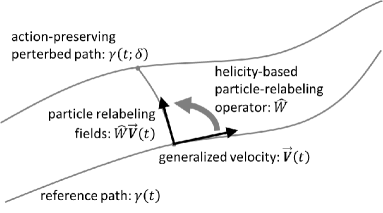
Figure 1: Relation among generalized velocity, $\vec{\bm{V}}$, helicity-based, particle-relabeling operator, $\hat{W}$, and action-preserving path variation, $\gamma(t)\to\gamma(t;\delta)$.

As is shown in the previous section, the pair of vector fields ($\alpha C_{i}{[d\underline{\bm{M}_{i}}]}$, $\alpha C_{e}{[d\underline{\bm{M}_{e}}]}$) satisfies the particle relabeling symmetry conditions (19). This implies that the integral path in the configuration space shifted in this direction retains the value of the action. Noticing that the vector fields pair is obtained by operation of appropriate operator on the ion and electron velocities pair as follows:

$$\left(\begin{array}[]{c}\alpha C_{i}{[d\underline{\bm{M}_{i}}]}\Big{.}\\ \alpha C_{e}{[d\underline{\bm{M}_{e}}]}\Big{.}\end{array}\right)=\hat{W}\left(\begin{array}[]{c}{\bm{V}_{i}}\Big{.}\\ {\bm{V}_{e}}\Big{.}\end{array}\right),$$ (41)

where the integro-differential operator, $\hat{W}$, is defined by

$$\hat{W}:=\left(\begin{array}[]{cc}C_{i}(\alpha\nabla\times)^{-1}+C_{i}\alpha\nabla\times&-C_{i}(\alpha\nabla\times)^{-1}\\ -C_{e}(\alpha\nabla\times)^{-1}&C_{e}(\alpha\nabla\times)^{-1}\end{array}\right),\hskip 10.00002pt$$ (44)

we recognize that the operation of  $\hat{W}$ on the integral path of the action physically implies infinitesimal particle relabeling operation (see Fig.1). Thus, we call $\hat{W}$ helicity-based, particle-relabeling operator hereafter.

It seems reasonable to consider the eigenvalue problem of the operator $\hat{W}$, because it is expected that the spectral expansion by such eigenfunctions should have some “good” properties for the description of the basic formulas and equations. In the following, we will solve the eigenvalue problem, demonstrate the mode expansions of various quantities and equations, and discuss the relation to the uniform background magnetic field effect and the standard MHD limit.

The eigenvalue problem of the operator,

$$\hat{W}\vec{\bm{V}}=\Lambda\vec{\bm{V}},$$ (45)

is equivalent to the double Beltrami flow (DBF) problem, which is given by the following coupled partial differential equations Mahajan and Yoshida (1998);

$$\alpha\nabla\times\bm{u}+\bm{b}=\frac{\Lambda}{C_{i}}\bm{u}, \bm{b}=-\frac{\Lambda}{C_{e}}(\bm{u}-\alpha\bm{j}).$$ (46)

Note that the eigenfunction of the DBF problem is constructed using a Beltrami flow, i.e., the eigenfunctions of the curl operator, say ${\bm{\psi}}(\vec{K},\sigma)$, which satisfies

$$\nabla\times{\bm{\psi}}(\vec{K},\sigma)=\sigma K{\bm{\psi}}(\vec{K},\sigma),$$

where $\vec{K}$, $K>0$, and $\sigma=\pm 1$ are the mode index, the associated eivenvalue, and the helicity of vector field, respectively . The Chandrasekhar-Kendall function on a cylindrical configuration Chandrasekhar and Kendall (1957) and the complex helical waves on a periodic box or a Euclidean space Waleffe (1992) are known as examples of the Beltrami flows. Expanding the variables using ${\bm{\psi}}(\vec{K},\sigma)$, the operator $\hat{W}$ is reduced to a 2$\times$2 matrix as

$$\sigma\left(\begin{array}[]{cc}\displaystyle\bigg{.}\frac{C_{i}}{\alpha K}+C_{i}\alpha K&\displaystyle-\frac{C_{i}}{\alpha K}\\ \displaystyle\bigg{.}-\frac{C_{e}}{\alpha K}&\displaystyle\frac{C_{e}}{\alpha K}\end{array}\right),$$

for each expansion mode. The eigenvalue of this matrix is given by

$$\Lambda(K,\sigma,s) = \frac{\sigma}{2}\bigg{\{}\frac{C_{i}+C_{e}}{\alpha K}+C_{i}\alpha K$$ (47)

$$+s\Big{[}\big{(}\frac{C_{i}+C_{e}}{\alpha K}-C_{i}\alpha K\big{)}^{2}+4C_{i}^{2}\Big{]}^{\frac{1}{2}}\bigg{\}},\hskip 10.00002pt$$

where $s=\pm 1$ is the polarity. Note that, the eigenvalues for the assigned $K$ and $\sigma$ satisfy

$$\Lambda(K,\sigma,+)\Lambda(K,\sigma,-)=C_{i}C_{e},$$ (48)

and, in the standard MHD limit $\alpha\to 0$, they become

$$\Lambda(K,\sigma,+)\to\infty,\ \Lambda(K,\sigma,-)\to 0 C_{i}\neq-C_{e},\ \$$   for (49)

$$\Lambda(K,\sigma,s)\to\sigma s|C_{i}| C_{i}=-C_{e}.\ \$$   for (50)

The eigenfunction of $\hat{W}$, say ${\vec{\bm{\Psi}}}={}^{t}({\bm{\Psi}{{}_{i}}},{\bm{\Psi}{{}_{e}}}),$ is given by

$${\vec{\bm{\Psi}}}{(\vec{K},\sigma,s)} = \left(\begin{array}[]{c}\left(\frac{1}{{\Lambda}(\vec{K},\sigma,s)}-\frac{\alpha K}{\sigma C_{e}}\right){\bm{\psi}}(\vec{K},\sigma)\\ \frac{1}{{\Lambda}(\vec{K},\sigma,s)}{\bm{\psi}}(\vec{K},\sigma)\end{array}\right),$$ (53)

and we call the set of the eigenfunctions the DBF basis, hereafter. If the Beltrami functions ${\bm{\psi}}$ are orthonormal each other:

$$\int{\bm{\psi}}(\vec{K},\sigma_{K})\cdot\overline{{\bm{\psi}}(\vec{P},\sigma_{P})}\,{\rm{d}}^{3}\vec{x} = \delta_{\vec{K},\vec{P}}\,\delta_{\sigma_{K},\sigma_{P}},$$ (54)

hereafter, overline and $\delta$ denote complex conjugate and Kronecker’s delta, respectively. The corresponding eigenfunctions $\vec{\bm{\Psi}}$ are orthogonal:

$${\Big{<}}\vec{\bm{\Psi}}(\widetilde{K}){\Big{|}}\overline{\vec{\bm{\Psi}}(\widetilde{P})}{\Big{>}} = g(\widetilde{K})\,\delta_{\vec{K},\vec{P}}\,\delta_{\sigma_{K},\sigma_{P}}\,\delta_{s_{K},s_{P}},\hskip 20.00003pt$$ (55)

hereafter, the tilde denotes the set of mode indices, $\widetilde{K}:=(\vec{K},\sigma_{K},s_{K})$, and $g$ is the inner product of the base function ${\vec{\bm{\Psi}}}{(\widetilde{K}{})}$, i.e., mathematically the component of the Riemannian metric tensor (9) for the DBF basis, that is to say

$$g(\widetilde{K}) := \left(\frac{1}{{\Lambda}(\widetilde{K})}-\frac{\alpha K}{\sigma_{K}C_{e}}\right)^{2}+\frac{1}{C_{e}^{2}}.$$ (56)

Substitution of $\bm{\Psi}{{}_{i}}$ and $\bm{\Psi}{{}_{e}}$ into (18) yields the base functions of conjugate momenta space, say $\underline{\vec{\bm{\Psi}}}={}^{t}(\underline{\bm{\Psi}_{i}},\underline{\bm{\Psi}_{e}}),$ as follows:

$$\underline{\vec{\bm{\Psi}}}{(\widetilde{K})} = \left(\begin{array}[]{c}\left(\frac{1}{{\Lambda}(\widetilde{K})}-\frac{\alpha K}{\sigma C_{e}}-\frac{\sigma}{C_{e}\alpha K}\right){\bm{\psi}}(\vec{K},\sigma)\\ \frac{\sigma}{C_{e}\alpha K}{\bm{\psi}}(\vec{K},\sigma)\end{array}\right).\hskip 10.00002pt$$ (59)

It is easy to check that the base functions ${\vec{\bm{\Psi}}}$ and $\underline{\vec{\bm{\Psi}}}$ are bi-orthogonal each other; i.e.,

$${\big{(}}\underline{\bm{\Psi}_{i}}{(\widetilde{K})}{\big{|}}{\bm{\Psi}_{i}}{(\widetilde{P})}{\big{)}}+{\big{(}}\underline{\bm{\Psi}_{e}}{(\widetilde{K})}{\big{|}}{\bm{\Psi}_{e}}{(\widetilde{P})}{\big{)}}$$

$$=g(\widetilde{K})\,\delta_{\vec{K},\vec{P}}\,\delta_{\sigma_{K},\sigma_{P}}\,\delta_{s_{K},s_{P}}.$$ (60)

Using these base functions, we can rewrite the eigenvalue problem (45) as follows:

$$\left(\begin{array}[]{c}\alpha C_{i}\nabla\times\underline{\bm{\Psi}_{i}}(\widetilde{K})\\ \alpha C_{e}\nabla\times\underline{\bm{\Psi}_{e}}(\widetilde{K})\end{array}\right)={\Lambda}(\widetilde{K})\left(\begin{array}[]{c}{\bm{\Psi}_{i}}(\widetilde{K})\\ {\bm{\Psi}_{e}}(\widetilde{K})\end{array}\right).$$ (65)

The generalized velocity and momentum are expanded using the eigenfunctions of $\hat{W}$ as

$$\vec{\bm{V}}=\sum_{\widetilde{K}}\widehat{V}(\widetilde{K})\,\vec{\bm{\Psi}}(\widetilde{K}), \vec{\bm{M}}=\sum_{\widetilde{K}}\widehat{V}(\widetilde{K})\,\underline{\vec{\bm{\Psi}}}(\widetilde{K}),$$ (66)

where the expansion coeffcient, $\widehat{V}(\widetilde{K})$, is obtained by the inner product,

$$\widehat{V}(\tilde{K}) = {\Big{<}}\vec{\bm{V}}{\Big{|}}\,\overline{\vec{\bm{\Psi}}(\tilde{K})}\,{\Big{>}}.$$ (67)

Since $\bm{V}_{i}=\bm{u}$ and $\alpha\nabla\times\underline{\bm{M}_{e}}=\alpha\nabla\times(\bm{a}/\alpha)=-\bm{b}$, the expansion coefficients, $\widehat{V}(\vec{K},\sigma,s)$, are determined by the following simultaneous equations:

$$\widehat{u}(\vec{K},\sigma) = \left(\frac{1}{{\Lambda}(K,\sigma,+)}-\frac{\alpha K}{\sigma C_{e}}\right)\widehat{V}(\vec{K},\sigma,+)$$

$$+\left(\frac{1}{{\Lambda}(K,\sigma,-)}-\frac{\alpha K}{\sigma C_{e}}\right)\widehat{V}(\vec{K},\sigma,-),$$

$$\widehat{b}(\vec{K},\sigma) = -\frac{1}{C_{e}}\left(\widehat{V}(\vec{K},\sigma,+)+\widehat{V}(\vec{K},\sigma,-)\right),$$ (68)

where $\widehat{u}(\vec{K},\sigma)$ and $\widehat{b}(\vec{K},\sigma)$ are the spectral expansion coefficients of the velocity and magnetic fields with respect to the basis $\{{\bm{\psi}}(\vec{K},\sigma)\}$, respectively. Unfortunately, the expansion coefficients $\widehat{V}$ converge to zero or diverge in the limit $\alpha\to 0$, unless $C_{i}=-C_{e}$.

The energy and the mixed helicity are obtained by substituting (66) into (12) and (34) and using the relations (55), (60), and (65); i.e.,

$$E = \frac{1}{2}{\Big{<}}\sum\widehat{V}(\tilde{K}){\vec{\bm{\Psi}}}(\tilde{K}){\Big{|}}\sum\widehat{V}(\tilde{P}){\vec{\bm{\Psi}}}(\tilde{P}){\Big{>}}$$ (69)

$$= \frac{1}{2}\sum_{\tilde{K}}g(\tilde{K})\left|\widehat{V}(\tilde{K})\right|^{2},$$

$$H = \alpha C_{i}{\Big{(}}\sum\widehat{V}(\tilde{K})\underline{\bm{\Psi}_{i}}(\tilde{K}){\Big{|}}\sum\widehat{V}(\tilde{P})\nabla\times\underline{\bm{\Psi}_{i}}(\tilde{P}){\Big{)}}$$ (70)

$$+\alpha C_{e}{\Big{(}}\sum\widehat{V}(\tilde{K})\underline{\bm{\Psi}_{e}}(\tilde{K}){\Big{|}}\sum\widehat{V}(\tilde{P})\nabla\times\underline{\bm{\Psi}_{e}}(\tilde{P}){\Big{)}}$$

$$= \sum_{\tilde{K}}g(\tilde{K})\Lambda(\tilde{K})\left|\widehat{V}(\tilde{K})\right|^{2}.$$

Applying the DBF expansion to the equation of motion yields the following simultaneous equations for the expansion coefficients, ${\widehat{V}(\tilde{K}{};t)}$:

$$\frac{{\rm{d}}}{{\rm{d}}t}\overline{\widehat{V}(\tilde{K}{};t)}=g(\tilde{K}{})^{-1}\sum_{\tilde{P}{}}\sum_{\tilde{Q}{}} {\big{(}}\!{\big{(}}\tilde{K}{}{\big{|}}\!{\big{|}}\tilde{P}{}{\big{|}}\!{\big{|}}\tilde{Q}{}{\big{)}}\!{\big{)}}\,\Lambda(\tilde{Q}{})\,$$ (71)

$$\times\widehat{V}(\tilde{P}{};t)\,\widehat{V}(\tilde{Q}{};t),$$

where the symbol ${\big{(}}\!{\big{(}}\tilde{K}{}{\big{|}}\!{\big{|}}\tilde{P}{}{\big{|}}\!{\big{|}}\tilde{Q}{}{\big{)}}\!{\big{)}}$ is given by

$${\big{(}}\!{\big{(}}\tilde{K}{}{\big{|}}\!{\big{|}}\tilde{P}{}{\big{|}}\!{\big{|}}\tilde{Q}{}{\big{)}}\!{\big{)}} =\frac{1}{\alpha}\Bigg{[}\frac{1}{C_{i}}\bigg{(}\frac{1}{{\Lambda}(\tilde{K}{})}-\frac{\alpha K}{\sigma_{K}C_{e}}\bigg{)}\bigg{(}\frac{1}{{\Lambda}(\tilde{P}{})}-\frac{\alpha P}{\sigma_{P}C_{e}}\bigg{)}$$

$$\times\bigg{(}\frac{1}{{\Lambda}(\tilde{Q}{})}-\frac{\alpha Q}{\sigma_{Q}C_{e}}\bigg{)}+\frac{1}{C_{e}\Lambda(\tilde{K}{})\Lambda(\tilde{P}{})\Lambda(\tilde{Q}{})}\Bigg{]}$$

$$\times\int{\bm{\psi}}(\vec{K},\sigma_{K})\cdot\left({\bm{\psi}}(\vec{P},\sigma_{P})\times{\bm{\psi}}(\vec{Q},\sigma_{Q})\right){\rm{d}}^{3}\vec{x}.$$

The derivations of (71) and (LABEL:str._const._core_DCB) are summarized in Appendix C. Note that the symbol ${\big{(}}\!{\big{(}}\tilde{K}{}{\big{|}}\!{\big{|}}\tilde{P}{}{\big{|}}\!{\big{|}}\tilde{Q}{}{\big{)}}\!{\big{)}}$ is skew-symmetric between two arbitrary argument sets, because the integrand is given by a scalar triple product of vector-valued functions whereas the coefficient is symmetric. Due to this skew symmetry, we can easily prove the conservation laws of the energy and the mixed helicity from the expression (71) as follows:

$$\frac{{\rm{d}}E}{{\rm{d}}t}= \frac{1}{2}\sum_{\tilde{K}{}}\sum_{\tilde{P}{}}\sum_{\tilde{Q}{}}{\big{(}}\!{\big{(}}\tilde{K}{}{\big{|}}\!{\big{|}}\tilde{P}{}{\big{|}}\!{\big{|}}\tilde{Q}{}{\big{)}}\!{\big{)}}\,\Lambda(\tilde{Q}{})\,$$ (73)

$$\hskip 10.00002pt\times\widehat{V}(\tilde{K}{};t)\,\widehat{V}(\tilde{P}{};t)\,\widehat{V}(\tilde{Q}{};t)+c.c.=0,\hskip 10.00002pt$$

$$\frac{{\rm{d}}H}{{\rm{d}}t}= \sum_{\tilde{K}{}}\sum_{\tilde{P}{}}\sum_{\tilde{Q}{}}{\big{(}}\!{\big{(}}\tilde{K}{}{\big{|}}\!{\big{|}}\tilde{P}{}{\big{|}}\!{\big{|}}\tilde{Q}{}{\big{)}}\!{\big{)}}\,\Lambda(\tilde{K}{})\,\Lambda(\tilde{Q}{})\,$$ (74)

$$\hskip 10.00002pt\times\widehat{V}(\tilde{K}{};t)\,\widehat{V}(\tilde{P}{};t)\,\widehat{V}(\tilde{Q}{};t)+c.c.=0.$$

Thus, the DBFs, i.e., the eigenfunctions of the helicity-based particle-relabeling operator are shown to constitute a family of orthogonal function bases that yields a remarkably simple spectral representation of the equation of motion. Especially, the mixed helicity conservation is naturally built in this representation due to the skew-symmetry of the coefficients of the quadratic terms. In the previous study, wherein the generalized Elsässer variables (GEV) expansion of the HMHD system was presented, we conjectured that the conservation of the modified cross helicity might reflect some symmetry intrinsic in the system Araki (2015). Since the DBFs become the GEVs for $C_{i}=-C_{e}=1$, the modified helicity conservation is now recognized as the consequence of a special case of the particle relabeling symmetry for ion and electron flows.

VI Consideration of the uniform background magnetic field

For some practical applications, it is important to consider the influence of the uniform background magnetic field on the dynamics of plasmas.

Here, we mathematically consider the influence of a background magnetic field, say $\bm{B}_{0}$, which is a harmonic function: $\nabla\times\bm{B}_{0}=\bm{0}$, $\nabla\cdot\bm{B}_{0}={0}$. Substitution of $\bm{b}+\bm{B}_{0}$ into the equations of motion (33) yields

$$\begin{array}[]{l}(\partial_{t}+L_{\bm{V}_{i}})(\alpha[d\underline{\bm{M}_{i}}]+\bm{B}_{0})=\bm{0},\Big{.}\\ (\partial_{t}+L_{\bm{V}_{e}})(\alpha[d\underline{\bm{M}_{e}}]-\bm{B}_{0})=\bm{0}.\Big{.}\end{array}$$ (77)

When the amplitudes of the variables are sufficiently small compared to the modulus of $\bm{B}_{0}$, these equations are approximated as

$$\alpha\partial_{t}\big{[}d\underline{\bm{M}_{i}}\big{]}=L_{\bm{B}_{0}}{\bm{V}_{i}},\hskip 10.00002pt \alpha\partial_{t}\big{[}d\underline{\bm{M}_{e}}\big{]}=-L_{\bm{B}_{0}}{\bm{V}_{e}},$$ (78)

where the identity for two vector fields $L_{\bm{\xi}}{\bm{\eta}}=-L_{\bm{\eta}}{\bm{\xi}}$ is used (see Eq.(27)). These linear simultaneous equations can be described using the operator $\hat{W}$ as:

$$\frac{\partial}{\partial t}\hat{W}\left(\begin{array}[]{c}{\bm{V}_{i}}\\ {\bm{V}_{e}}\end{array}\right)=L_{\bm{B}_{0}}\left(\begin{array}[]{c}{\bm{V}_{i}}\\ {\bm{V}_{e}}\end{array}\right).$$ (83)

Thus, the linear waves are shown to be expressed by the eigenfunctions of the DBF problem (53), with $C_{i}=1$ and $C_{e}=-1$. The eigenvalue become

$$\Lambda(\tilde{K})=\frac{\sigma}{2}(\alpha K+s\sqrt{(\alpha K)^{2}+4}).$$

For typical velocity and magnetic field variables, the linear simultaneous equations are given by

$$\begin{array}[]{l}{{\partial_{t}}{\bm{u}}}=\bm{j}\times\bm{B}_{0}-\nabla P,\Big{.}\\ {{\partial_{t}}{\bm{b}}}=\nabla\times\big{(}(\bm{u}-\alpha\nabla\times\bm{b})\times\bm{B}_{0}\big{)}.\Big{.}\end{array}$$ (86)

The eigenfunctions of the linearized HMHD system (86) are known as the generalized Elsässer variables (GEV) Galtier (2006). Physically, the GEVs describe the ion cyclotron or whistler waves in plasmas. The phase velocity for an assigned $\tilde{K}$ is $\omega(\tilde{K}):=B_{0}k_{\parallel}\Lambda(\tilde{K})^{-1},$ where $k_{\parallel}$ is the wavenumber of ${\bm{\psi}}(\vec{K},\sigma_{K})$ in the direction of $\bm{B}_{0}$. The equations of motion for this case are obtained by substituting $\widehat{V}(\tilde{K};t)e^{-i\omega(\tilde{K})t}$ into $\widehat{V}(\tilde{K};t)$.

It is interesting that the GEV expansion coefficients of the basic variables are simply and hierarchically expressed by $\widehat{V}$ multiplied by the powers of $\Lambda$ as follows:

$$\begin{array}[]{rcl}\bm{V}_{e}&=&\bm{u}-\alpha\nabla\times\bm{b}\\ &=&\sum_{\tilde{K}{}}{\Lambda}(\tilde{K}{})^{-1}\ \widehat{V}(\tilde{K}{})\ {\bm{\psi}}(\vec{K},\sigma_{K}),\\ \\ -\alpha[d\underline{\bm{M}_{e}}]&=&\bm{b}\\ &=&\sum_{\tilde{K}{}}\widehat{V}(\tilde{K}{})\ {\bm{\psi}}(\vec{K},\sigma_{K}),\\ \\ \bm{V}_{i}&=&\bm{u}\\ &=&\sum_{\tilde{K}{}}{\Lambda}(\tilde{K}{})\ \widehat{V}(\tilde{K}{})\ {\bm{\psi}}(\vec{K},\sigma_{K}),\\ \\ \alpha[d\underline{\bm{M}_{i}}]&=&\alpha\nabla\times\bm{u}+\bm{b}\\ &=&\sum_{\tilde{K}{}}{\Lambda}(\tilde{K}{})^{2}\ \widehat{V}(\tilde{K}{})\ {\bm{\psi}}(\vec{K},\sigma_{K}).\end{array}$$ (98)

Note that helicity parameters for the linear wave modes have the following significant properties.

Firstly, the eigenvalues (47) do not diverge in the standard MHD limit, $\alpha\to 0$:

$$\Lambda(\tilde{K}{})\approx\sigma_{K}s_{K}+\frac{\alpha}{2}\sigma_{K}K+\frac{\alpha^{2}}{8}\sigma_{K}s_{K}K^{2}\longrightarrow\sigma_{K}s_{K}.$$

This convergence leads to the finiteness of the following quantities in that limit: coefficients of the base functions (53):

$${\vec{\bm{\Psi}}}{(\tilde{K}{})} \approx\left(\begin{array}[]{r}(\sigma_{K}s_{K}+\frac{\alpha}{2}\sigma_{K}K){\bm{\psi}}(\vec{K},\sigma_{K})\\ (\sigma_{K}s_{K}-\frac{\alpha}{2}\sigma_{K}K){\bm{\psi}}(\vec{K},\sigma_{K})\end{array}\right)$$ (104)

$$\longrightarrow\sigma_{K}s_{K}\left(\begin{array}[]{r}{\bm{\psi}}(\vec{K},\sigma_{K})\\ {\bm{\psi}}(\vec{K},\sigma_{K})\end{array}\right),$$

the Riemannian metric (56):

$$g(\tilde{K}{})=2+{\alpha}^{2}K^{2}\longrightarrow 2,$$

the coefficient of the RHS of (LABEL:str._const._core_DCB):

$$\frac{1}{\alpha}\Bigg{[}\bigg{(}\frac{1}{{\Lambda}(\tilde{K}{})}+\frac{\alpha K}{\sigma_{K}}\bigg{)}\bigg{(}\frac{1}{{\Lambda}(\tilde{P}{})}+\frac{\alpha P}{\sigma_{P}}\bigg{)}\bigg{(}\frac{1}{{\Lambda}(\tilde{Q}{})}+\frac{\alpha Q}{\sigma_{Q}}\bigg{)}$$

$$\hskip 10.00002pt-\frac{1}{\Lambda(\tilde{K}{})\Lambda(\tilde{P}{})\Lambda(\tilde{Q}{})}\Bigg{]}$$

$$\approx\sigma_{K}\sigma_{P}\sigma_{Q}s_{K}s_{P}s_{Q}\bigg{(}s_{K}K+s_{P}P+s_{Q}Q\bigg{)}$$

$$\hskip 10.00002pt+\frac{1}{8}\alpha^{2}\sigma_{K}\sigma_{P}\sigma_{Q}KPQ\bigg{(}\frac{s_{P}P+s_{Q}Q}{s_{K}K}$$

$$\hskip 30.00005pt+\frac{s_{Q}Q+s_{K}K}{s_{P}P}+\frac{s_{K}K+s_{P}P}{s_{Q}Q}+2\bigg{)}+o(\alpha^{2})$$

$$\longrightarrow\sigma_{K}\sigma_{P}\sigma_{Q}s_{K}s_{P}s_{Q}\bigg{(}s_{K}K+s_{P}P+s_{Q}Q\bigg{)}.$$ (105)

Since the simultaneous equations (68) converge to

$$\widehat{u}(\vec{K},\sigma_{K})=\sigma_{K}s_{K}\widehat{V}(\vec{K},\sigma_{K},-)-\sigma_{K}s_{K}\widehat{V}(\vec{K},\sigma_{K},+),$$

$$\widehat{b}(\vec{K},\sigma_{K})=\widehat{V}(\vec{K},\sigma_{K},+)+\widehat{V}(\vec{K},\sigma_{K},-),$$ (106)

we obtain the MHD limit of the expansion coefficient, $\widehat{V}$:

$$\widehat{V}(\tilde{K}{},\sigma_{K},s_{K})=\widehat{b}(\vec{K},\sigma_{K})-\sigma_{K}s_{K}\,\widehat{u}(\vec{K},\sigma_{K}),$$ (107)

and thus, the equation of motion (71) has the standard MHD limit. The coefficients, $\widehat{V}$, are associated with the conventional Elsässer variables by the formula

$$\begin{array}[]{rcl}\bm{z}_{+}&=&\bm{u}+\bm{b}\\ &=&\widehat{V}(K,+,-){\bm{\psi}}(K,+)+\widehat{V}(K,-,+){\bm{\psi}}(K,-),\\ \bm{z}_{-}&=&\bm{u}-\bm{b}\\ &=&-\widehat{V}(K,+,+){\bm{\psi}}(K,+)-\widehat{V}(K,-,-){\bm{\psi}}(K,-).\end{array}\hskip 10.00002pt$$ (112)

The base function in momentum space $\underline{\vec{\bm{\Psi}}}$, on the other hand, diverges on the order of $\alpha^{-1}$, at which the diverging $\bm{a}/\alpha$ term is reflected.

Secondly, the singularity order of the mixed helicity (34) reduces by $\alpha$ and the constant $H$ become the modified cross helicity, which converges to the cross helicity:

$$H_{C} =\int{\rm{d}}^{3}{\vec{x}}\,\big{[}2\bm{u}\cdot\bm{b}+\alpha\bm{u}\cdot(\nabla\times\bm{u})\big{]}$$ (113)

$$\longrightarrow 2\int{\rm{d}}^{3}{\vec{x}}\ \bm{u}\cdot\bm{b}.$$

In our previous study, it was shown that the conservation of the modified cross helicity is naturally derived from the GEV representation of the HMHD dynamics.

VII Discussion

In the present study, we considered the helicity conservation laws of HMHD system from Lagrangian mechanical, invariant action theory viewpoint. The hybrid and magnetic helicity conservation laws were derived as consequences of the particle relabeling symmetry of the ion and electron flows, respectively. To prove the conservation laws, it is convenient to use the pair of ion and electron velocity fields (7) as basic variables, while that of fluid velocity and current fields had been used in our previous study Araki (2015). Mathematically, this variables change was carried out by changing the configuration space of HMHD system from semidirect product group to direct product one.

Furthermore, associated integral path variation of the invariant action was shown to be expressed by the operation of the helicity-based, particle-relabeling operator (44) on the reference path, which maps the generalized velocities $(\bm{V}_{i},\bm{V}_{e})$ to the action-preserving, particle-relabeling fields $(\alpha C_{i}{[d\underline{\bm{M}_{i}}]},\alpha C_{e}{[d\underline{\bm{M}_{e}}]})$.

The eigenfunctions of the relabeling operator are DBFs, which are well-known, force-free solutions of the HMHD system Mahajan and Yoshida (1998), and found to provide a family of orthogonal function bases that yields the spectral representation of the equation of motion with a remarkably simple form. Thus, the GEV based formulation we had discussed in Araki (2015) is now understood as an example of more wider class of orthogonal function expansion of the HMHD equations, since the GEVs are special case of the DBFs ($C_{i}=-C_{e}=1$).

The implication of this eigenvalue problem may be well-understood by considering the correspondence between the Lagrangian and Hamiltonian mechanics.

It is well-known that the Lie algebraic structure naturally induces a so-called Lie-Poisson structure on the dual space of the Lie algebra by defining the Poisson bracket by ${\{}A,B{\}}(\mu)={\big{(}}\mu{\big{|}}{[}\frac{\partial A}{\partial\mu},\frac{\partial B}{\partial\mu}{]}{\big{)}},$ where $\mu\in\mathfrak{g}^{*}$ is an element of the generalized momentum space, and $A,\,B\in{\cal{F}}(\mathfrak{g}^{*})$ are the functionals of the generalized momenta Marsden and Ratiu (1994). In the incompressible HMHD case, the Poisson bracket based on (8) and (9) becomes

$${\big{\{}}A,B{\big{\}}}(\vec{\bm{M}}) = {\Big{(}}\bm{M}_{i}{\Big{|}}\nabla\times\big{(}\frac{\delta A}{\delta\bm{M}_{i}}\times\frac{\delta B}{\delta\bm{M}_{i}}\big{)}{\Big{)}}$$ (114)

$$+{\Big{(}}\bm{M}_{e}{\Big{|}}\nabla\times\big{(}\frac{\delta A}{\delta\bm{M}_{e}}\times\frac{\delta B}{\delta\bm{M}_{e}}\big{)}{\Big{)}}.$$

When $B$ is the Hamiltonian obtained by the Legendre transformation of the Lagrangian (12), which results in $B(\vec{\bm{M}})=L(\vec{\bm{V}})$, the functional derivatives of $B$ are given by $\frac{\delta B}{\delta\bm{M}_{i}}=\bm{V}_{i},$ $\frac{\delta B}{\delta\bm{M}_{e}}=\bm{V}_{e}.$ Integration by parts of (114) yields

$${\big{\{}}A,B{\big{\}}}(\vec{\bm{M}}) = \int{\rm{d}}^{3}\vec{x}\bigg{[}\frac{\delta A}{\delta\bm{M}_{i}}\cdot\Big{(}\bm{V}_{i}\times\big{(}\nabla\times\bm{M}_{i}\big{)}\Big{)}$$ (115)

$$\hskip 30.00005pt+\frac{\delta A}{\delta\bm{M}_{e}}\cdot\Big{(}\bm{V}_{e}\times\big{(}\nabla\times\bm{M}_{e}\big{)}\Big{)}\bigg{]}.\hskip 10.00002pt$$

By setting the derivatives $\frac{\delta A}{\delta\bm{M}_{i}}=\bm{\xi},$ $\frac{\delta A}{\delta\bm{M}_{e}}=\bm{\eta},$ the cubic terms of the first variation (21) are reproduced, and thus, the action-preserving variation is shown to correspond to the functional derivative of a certain Casimir function.

In the Hamiltonian mechanical approach to the stability problem of the equilibrium solutions, the DBF are known to constitute the dynamically accessible variations that a priori satisfy the conservation laws for energy and Casimirs Hirota et al. (2006). In the incompressible HMHD case, the Casimirs are given by the magnetic and hybrid helicities. In the Lagrangian mechanical approach, on the other hand, they are obtained from the invariant action. Thus, the eigenvalue problem for the invariant action is naturally described as the DBF problem.

Since the DBFs for assigned $C_{i}$ and $C_{e}$ were orthogonal each other, by using them as base functions we could obtain a general form of the “normal mode” expansion of the Riemannian metric, the structure constants of the Lie algebra, and the equation of motion. The combinations of $C_{i}$ and $C_{e}$ are arbitrary, i.e., the DBF basis has two degrees of freedom. By changing the values of $C_{i}$ and $C_{e}$, we obtained a family of “canonical” transformations between the spectral representations of the equation of motion. The spectral representations of the equation of motion formally have a common mathematical expression given by (71), which is known as the Euler-Poincare equation (Chapter 13 of Ref.Marsden and Ratiu (1994)), or as the geodesic equation Arnold (1966);

$$\frac{{\rm{d}}}{{\rm{d}}t}\frac{\partial l}{\partial\xi^{a}}=C_{da}^{b}\xi^{d}\frac{\partial l}{\partial\xi^{b}},$$

where the variables and coefficients ${\xi}^{d}$, $\frac{\partial l}{\partial\xi^{a}}$, $C_{da}^{b}$ respectively correspond to $\vec{\bm{V}}(\tilde{K}{})$, $\vec{\bm{M}}(\tilde{K}{})$, and ${(}\!{(}\tilde{K}{}{|}\!{|}\tilde{P}{}{|}\!{|}\tilde{Q}{}{)}\!{)}\Lambda(\tilde{K}{})/g(\tilde{K}{})$ in the present study. As is expected, conservation laws for the energy and the mixed helicity are easily proved from the symmetric properties of the obtained structure constant.

In the standard MHD limit $\alpha\to 0$, the eigenvalues, and thus, the related quantities such as the expansion coefficients, the Riemannian metric, and the structure constants, diverge or shrink to zero unless $C_{i}=-C_{e}$. Hence, the DBF basis seems unsuitable for comparative analysis between HMHD and MHD in most cases. However, it is very interesting that consideration of the effect of a uniform background magnetic field yields such a linear wave equation that uses the same DBF operator as $C_{i}=-C_{e}=1.$ It is well-known that the linear wave modes in the incompressible HMHD system are the ion cyclotron and whistler waves and are elegantly described by the GEV Galtier (2006). That is, the GEV is such that the DBF has non-diverging properties in the limit $\alpha\to 0.$ Thus, among the wide variety of the DBF expansions, the GEV expansion is the most suitable for comparing the dynamics of the HMHD system to its MHD limit, avoiding singularity problems.

Since the DBFs are constructed from the eigenfunctions of the curl operator, it is easy to include Laplacian-type dissipation into the spectral representation of the equation of motion;

$$\Big{(}g(\tilde{K}{})\frac{\partial}{\partial t}+D(\tilde{K}{},\nu,\eta)\Big{)}\overline{\widehat{V}(\tilde{K}{};t)}$$

$$\hskip 10.00002pt=\sum_{\tilde{P}{}}\sum_{\tilde{Q}{}}{\big{(}}\!{\big{(}}\tilde{K}{}{\big{|}}\!{\big{|}}\tilde{P}{}{\big{|}}\!{\big{|}}\tilde{Q}{}{\big{)}}\!{\big{)}}\,\Lambda(\tilde{Q}{})\,\widehat{V}(\tilde{P}{};t)\,\widehat{V}(\tilde{Q}{};t),$$ (116)

where $D$, $\nu$, and $\eta$ are the dissipation term coefficient given by

$$D(\tilde{K},\nu,\eta):={K^{2}}\left[\nu\left(\frac{1}{{\Lambda}(\tilde{K})}-\frac{\sigma_{K}K}{C_{e}}\right)^{2}+\frac{\eta}{C_{e}^{2}}\right],$$

the kinematic viscosity, and the resistivity, respectively. This feature allows us to apply the DBF expansion to such analyses as the closure problem Galtier (2006) or the direct numerical simulation Araki and Miura (2015).

Appendix A Derivation of the Lin constraints

We briefly review the derivation of the formula for the variation of the tangent vector to an integral path. For this derivation process, we use only the exponential map and the Baker-Campbell-Hausdorff formula. Since no material specific to any particular Lie algebra is used here, the result is applicable to all the Lie groups.

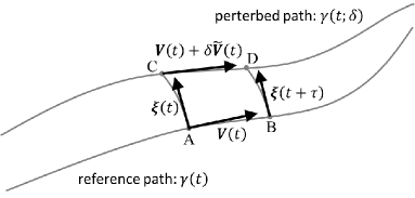
Figure 2: The derivation of the Lin constraints using approximations of short intervals on paths.

Let $\gamma(t;\delta)$ ($t\in[0,1]$) be a path on $G$ with a variation parameter $\delta\in I\in\mathbb{R}$. The path C$\to$D is approximated by

$\gamma(t+\tau;\delta)$ $\approx$ $\exp\big{[}\tau\big{(}\bm{V}(t)+\delta\tilde{\bm{V}}(t)\big{)}\big{]}$ $\circ$ $\gamma(t;\delta)$,

where ${\bm{V}}(t)$ is the tangent vector to the reference path ($\delta=0$), and $\delta\tilde{\bm{V}}(t)$ is the small deviation. The path C$\to$A$\to$B$\to$D is, on the other hand, also approximated by

$$\gamma(t+\tau;\delta) \approx \exp\big{(}\delta\bm{\xi}(t+\tau)\big{)}\circ\exp\big{(}\tau\bm{V}(t)\big{)}$$

$$\circ\exp\big{(}-\delta\bm{\xi}(t)\big{)}\circ\gamma(t;\delta)$$

(see Figure 2). Expanding $\bm{\xi}(t+\tau)=\bm{\xi}(t)+\tau{\partial_{t}}{\bm{\xi}}(t)+o(\tau)$ and using the Baker-Campbell-Hausdorff formula at the lowest two orders, we obtain

$$\exp\big{(}\delta\bm{\xi}(t+\tau)\big{)}\circ\exp\big{(}\tau\bm{V}(t)\big{)}\circ\exp\big{(}-\delta\bm{\xi}(t)\big{)}$$

$$=\exp\Big{[}\tau\bm{V}(t)+\tau\delta\big{(}{\partial_{t}}{\bm{\xi}}(t)+{[}\bm{\xi}(t),\bm{V}(t){]}\big{)}+o(\delta)+o(\tau)\Big{]}.$$

Since the two approximated paths from C to D agree with each other in the limit $\delta\to 0$ and $\tau\to 0$, we obtain the Lin constraints

$$\tilde{\bm{V}}(t)={\partial_{t}}{\bm{\xi}}(t)+{[}\bm{\xi}(t),\bm{V}(t){]}$$ (119)

at the order $O(\delta\tau)$.

Appendix B local expression of particle-relabeling symmetry

By the term “particle-relabeling symmetry,” we recognize the invariance of the flow against the change of Lagrangian coordinates. The freedom of choice of the action-preserving transformation exists only at the “initial time” and the transformation along the integral path of the action is determined by this initial condition. This symmetry is qualitatively different from the symmetry considered, for example, in gauge field theory, wherein, in principle, group transformation is applicable at any point in the relevant space and time Utiyama (1956).

Thus, the evolution of transformation should be considered. Let $\bm{\xi}$ and $\epsilon$ be a displacement-generating vector field and a small parameter, respectively. For an assigned flow and a sufficiently small displacement, the displacement field must satisfy the particle tracing relation:

$$\vec{X}\big{(}\vec{a}+\epsilon\bm{\xi}(\vec{a};0);t\big{)} = \vec{X}(\vec{a};t)+\epsilon\bm{\xi}\big{(}\vec{X}(\vec{a};t);t\big{)},$$ (120)

where the $\vec{X}$ is the PTM for the assigned flow. At the order $O(\epsilon)$, each component of $\bm{\xi}$ satisfies

$${\xi}^{k}(\vec{a};0)\left.\frac{\partial X^{i}}{\partial x^{k}}\right|_{(\vec{a};t)} = {\xi}^{i}\big{(}\vec{X}(\vec{a};t);t\big{)}.$$ (121)

Differentiating with respect to $t$ and evaluating at $t=0$, we obtain

$${\xi}^{k}(\vec{a};0)\left.\frac{\partial^{2}X^{i}}{\partial x^{k}\partial t}\right|_{(\vec{a};0)} = \left.\frac{\partial{\xi}^{i}}{\partial x^{k}}\right|_{(\vec{X}(\vec{a};0);0)}\left.\frac{\partial X^{k}}{\partial t}\right|_{(\vec{a};0)}$$ (122)

$$+\frac{\partial{\xi}^{i}}{\partial t}_{(\vec{X}(\vec{a};0);0)}.$$

The relation (7) leads to the following PDE for the vector fields in the Eulerian specification:

$$\left(\frac{\partial{\xi}^{i}}{\partial t}+V^{k}\frac{\partial{\xi}^{i}}{\partial x^{k}}-{\xi}^{k}\frac{\partial V^{i}}{\partial x^{k}}\right)_{(\vec{X}(\vec{a};0);0)}=0,$$ (123)

which is the evolution equation for the frozen-in line element. Since the Lie bracket of the vector fields is given by (27), the obtained evolution equation agrees with (119) for $\tilde{\bm{V}}(t)=\bm{0}$. For divergence-free fields in a three-dimensional space, the equation is rewritten using vector analysis notation as

$$\partial_{t}\bm{\xi}+\nabla\times(\bm{\xi}\times\bm{V})=\bm{0}.$$ (124)

Appendix C Structure constants for the DBF basis

The symbol ${\big{(}}\!{\big{(}}\tilde{K}{}{\big{|}}\!{\big{|}}\tilde{P}{}{\big{|}}\!{\big{|}}\tilde{Q}{}{\big{)}}\!{\big{)}}$, which is related to the structure constant of the Lie algebra, is defined by using a combination of the Riemannian metric and the Poisson bracket for the HMHD system as follows:

$${\big{(}}\!{\big{(}}\tilde{K}{}{\big{|}}\!{\big{|}}\tilde{P}{}{\big{|}}\!{\big{|}}\tilde{Q}{}{\big{)}}\!{\big{)}}\,{\Lambda}(\tilde{K}{}):={\Big{<}}\vec{\bm{\Psi}}{(\tilde{K}{})}{\Big{|}}{\big{[}}\vec{\bm{\Psi}}{(\tilde{P}{})},\vec{\bm{\Psi}}{(\tilde{Q}{})}{\big{]}}{\Big{>}}$$ (125)

$$= {\Big{(}}\underline{\bm{\Psi}_{i}}(\tilde{K}{}){\Big{|}}\nabla\times\big{(}\bm{\Psi}_{i}(\tilde{P}{})\times\bm{\Psi}_{i}(\tilde{Q}{})\big{)}{\Big{)}}$$

$$+{\Big{(}}\underline{\bm{\Psi}_{e}}(\tilde{K}{}){\Big{|}}\nabla\times\big{(}\bm{\Psi}_{e}(\tilde{P}{})\times\bm{\Psi}_{e}(\tilde{Q}{})\big{)}{\Big{)}}$$

$$= \frac{{\Lambda}(\tilde{K}{})}{\alpha}\int{\rm{d}}^{3}\vec{x}\Big{[}C_{i}^{-1}\bm{\Psi}_{i}(\tilde{K}{})\cdot\big{(}\bm{\Psi}_{i}(\tilde{P}{})\times\bm{\Psi}_{i}(\tilde{Q}{})\big{)}$$

$$\hskip 50.00008pt+C_{e}^{-1}\bm{\Psi}_{e}(\tilde{K}{})\cdot\big{(}\bm{\Psi}_{e}(\tilde{P}{})\times\bm{\Psi}_{e}(\tilde{Q}{})\big{)}\Big{]},\hskip 10.00002pt$$

where the second line is derived by integrating by parts with respect to $\vec{x}$ and by using the relation (65). Substitution of (53) into the second line yields (LABEL:str._const._core_DCB), i.e., the explicit expression of the symbol ${\big{(}}\!{\big{(}}\tilde{K}{}{\big{|}}\!{\big{|}}\tilde{P}{}{\big{|}}\!{\big{|}}\tilde{Q}{}{\big{)}}\!{\big{)}}.$ Using this symbol, the first variation of action reads as

$$\int_{0}^{1}dt{\Big{<}}\sum_{\tilde{Q}}\vec{\bm{V}}(\tilde{Q}{}){\Big{|}}\partial_{t}\vec{\bm{\xi}}(\tilde{K}{})+{\big{[}}\vec{\bm{\xi}}(\tilde{K}{}),\sum_{\tilde{P}}\vec{\bm{V}}{(\tilde{P}{})}{\big{]}}{\Big{>}}$$

$$=\int_{0}^{1}dt\Big{(}g(\tilde{K})\overline{\widehat{V}(\tilde{K}{})}\partial_{t}{\widehat{\xi}}(\tilde{K}{})$$

$$\hskip 40.00006pt+\sum_{\tilde{P},\tilde{Q}}\Lambda(\tilde{Q}{}){\big{(}}\!{\big{(}}\tilde{Q}{}{\big{|}}\!{\big{|}}\tilde{K}{}{\big{|}}\!{\big{|}}\tilde{P}{}{\big{)}}\!{\big{)}}\widehat{V}(\tilde{Q}{}){\widehat{\xi}}(\tilde{K}{})\widehat{V}(\tilde{P}{})\Big{)},$$

$$=\left(g(\tilde{K})\overline{\widehat{V}(\tilde{K}{})}{\widehat{\xi}}(\tilde{K}{})\right)_{t=1}-\left(g(\tilde{K})\overline{\widehat{V}(\tilde{K}{})}{\widehat{\xi}}(\tilde{K}{})\right)_{t=0}$$

$$\hskip 10.00002pt+\int_{0}^{1}dt{\widehat{\xi}}(\tilde{K}{})\Big{(}-g(\tilde{K})\partial_{t}\overline{{\widehat{V}}(\tilde{K}{})}$$

$$\hskip 50.00008pt+\sum_{\tilde{P},\tilde{Q}}\Lambda(\tilde{Q}{}){\big{(}}\!{\big{(}}\tilde{K}{}{\big{|}}\!{\big{|}}\tilde{P}{}{\big{|}}\!{\big{|}}\tilde{Q}{}{\big{)}}\!{\big{)}}\widehat{V}(\tilde{Q}{})\widehat{V}(\tilde{P}{})\Big{)}.\hskip 10.00002pt$$ (126)

We obtain the Euler-Lagrange equation (71) if the fixed path end conditions are imposed.

References

• Note (1) Despite that the term “magnetohydrodynamics” fundamentally means continuous fluid approximation models of the collective motions of ions and electrons Miyamoto (2000), in many literatures the term is used to indicate the reduced, one-fluid plasma model wherein the ion and electron momenta are averaged, the (averaged) ion charge number, $Z$, is often set to one, and the Lorentz force is formulated using these averaged quantities. In the present study we use the term “MHD” or “standard MHD” in this meaning.
• Lighthill (1960) M. J. Lighthill, Phil. Trans. R. Soc. Lond. A 252, 397 (1960).
• Turner (1986) L. Turner, IEEE Trans. Plasma Sci. 14, 849 (1986).
• Araki (2015) K. Araki, J. Phys. A: Math. Theor. 48, 175501 (2015).
• Padhye and Morrison (1996) N. Padhye and P. J. Morrison, Plasma Phys. Rep. 22, 869 (1996).
• Holm (1987) D. D. Holm, Phys. Fluids 30, 1310 (1987).
• Sahraoui et al. (2003) F. Sahraoui, G. Belmont,  and L. Rezeau, Phys. Plasmas 10, 1325 (2003).
• Hirota et al. (2006) M. Hirota, Z. Yoshida,  and E. Hameiri, Phys. Plasmas 13, 022107 (2006).
• Charidakos et al. (2014) I. K. Charidakos, M. Lingam, P. J. M. R. L. White,  and A. Wurm, Phys. Plasmas 21, 092118 (2014).
• Arnold (1966) V. Arnold, Ann. Inst. Fourier 16, 319 (1966).
• Arnold and Khesin (1998) V. I. Arnold and B. A. Khesin, Topological Methods in Hydrodynamics (Springer-Verlag, 1998).
• Marsden and Ratiu (1994) J. E. Marsden and T. S. Ratiu, Introduction to Mechanics and Symmetry (Springer-Verlag, 1994).
• Zeitlin and Kambe (1993) V. Zeitlin and T. Kambe, J. Phys. A: Math. Gen. 26, 5025 (1993).
• Hattori (1994) Y. Hattori, J. Phys. A: Math. Gen. 27, L21 (1994).
• Vizman (2001) C. Vizman, Rendiconti del Circolo Matematico di Palermo, Serie II, Supplemento 66, 199 (2001).
• Yoshida and Hameiri (2013) Z. Yoshida and E. Hameiri, J. Phys. A: Math. Theor. 46, 335502 (2013).
• Miura and Araki (2015) H. Miura and K. Araki, Phys. Plasmas 21, 072313 (2015).
• Araki and Miura (2013) K. Araki and H. Miura, Plasma Fusion Res. 8, 2401137 (2013).
• Mahajan and Yoshida (1998) S. M. Mahajan and Z. Yoshida, Phys. Rev. Lett. 81, 4863 (1998).
• Yoshida and Mahajan (2002) Z. Yoshida and S. M. Mahajan, Phys. Rev. Lett. 88, 095001 (2002).
• Galtier (2006) S. Galtier, J. Plasma Phys. 72, 721 (2006).
• Araki and Miura (2015) K. Araki and H. Miura, Plasma Fusion Res. 10, 3401030 (2015).
• Note (2) In this paper, we place an arrow above the symbol to denote the multifunctional character of mathematical quantities. For example, a diffeomorphism (a triplet of functions) is expressed by $\mathaccentV{vec}17E{X}=(X^{1},X^{2},X^{3})$, and a pair of vector fields by $\mathaccentV{vec}17E{\bm{V}}=(\bm{V}_{i},\bm{V}_{e})$. Boldface letters are used to denote vector fields on $M$.
• Araki (2009) K. Araki, J. Math-for-industry 1, 139 (2009).
• Salmon (1988) R. Salmon, Ann. Rev. Fluid Mech. 20, 225 (1988).
• Note (3) The Lie derivative of a differential 1-form is given by $L_{\bm{\xi}}{\bm{\eta}}=\left(\xi^{k}\frac{\partial\eta_{j}}{\partial x^{k}}+{\eta_{k}}\frac{\partial\xi^{k}}{\partial x^{j}}\right)dx^{j}$ for ${\bm{\eta}}=\eta_{j}dx^{j}\in\Omega_{1}(M).$ In vector analysis notation, $L_{\bm{\xi}}{\bm{\eta}}=-\bm{\xi}\times(\nabla\times\bm{\eta})+\nabla(\bm{\xi}\cdot\bm{\eta})$.
• Tur and Yanovsky (1993) A. V. Tur and V. V. Yanovsky, J. Fluid Mech. 248, 67 (1993).
• Note (4) The Lie derivative of a differential 2-form on a three-dimensional manifold is given by $L_{\bm{\xi}}\bm{\eta}=\left(\xi^{k}\frac{\partial\eta^{j}}{\partial x^{k}}-{\eta^{k}}\frac{\partial\xi^{j}}{\partial x^{k}}+{\eta^{j}}\frac{\partial\xi^{k}}{\partial x^{k}}\right)\epsilon_{jlm}dx^{l}\wedge dx^{m},$ for $\bm{\eta}=\epsilon_{jlm}{\eta^{j}}dx^{l}\wedge dx^{m}\in\Omega_{2}(M),$ where $\epsilon_{jlm}$ is the Levi-Civita symbol. Due to the divergence-free condition, transformation rule of the coefficients against the change of the local coordinate system is given by $\eta^{\prime j}(\mathaccentV{vec}17E{y})=\eta^{i}(\mathaccentV{vec}17E{x})\frac{\partial y^{j}}{\partial x^{i}}$ for both the vector field and differential 2-form.
• Khesin and Chekanov (1989) B. A. Khesin and Y. V. Chekanov, Physica D40, 119 (1989).
• Note (5) Since $(\nabla\times)^{2}=-\triangle$ for divergence-free vector fields, if the function is not harmonic, the value $K>0$ is determined by the eigenvalue of the Laplacian: $\triangle\bm{\psi}=-K^{2}\bm{\psi}$.
• Chandrasekhar and Kendall (1957) S. Chandrasekhar and P. C. Kendall, Astrophys. J. 126, 457 (1957).
• Waleffe (1992) F. Waleffe, Phys. Fluids A 4, 350 (1992).
• Utiyama (1956) R. Utiyama, Phys. Rev. 101, 1597 (1956).
• Miyamoto (2000) K. Miyamoto, Fundamentals of plasma physics and controlled fusion, Tech. Rep. (National Inst. for Fusion Science, Nagoya (Japan), 2000).