Localized Multiple Kernel Learning—A Convex Approach

Abstract

We propose a localized approach to multiple kernel learning that can be formulated as a convex optimization problem over a given cluster structure. For which we obtain generalization error guarantees and derive an optimization algorithm based on the Fenchel dual representation. Experiments on real-world datasets from the application domains of computational biology and computer vision show that convex localized multiple kernel learning can achieve higher prediction accuracies than its global and non-convex local counterparts.

Keywords: Multiple kernel learning, Localized algorithms, Generalization analysis

1 Introduction

Kernel-based methods such as support vector machines have found diverse applications due to their distinct merits such as the descent computational complexity, high usability, and the solid mathematical foundation [e.g., 44]. The performance of such algorithms, however, crucially depends on the involved kernel function as it intrinsically specifies the feature space where the learning process is implemented, and thus provides a similarity measure on the input space. Yet in the standard setting of these methods the choice of the involved kernel is typically left to the user.

A substantial step toward the complete automatization of kernel-based machine learning is achieved in Lanckriet et al. [32], who introduce the multiple kernel learning (MKL) framework [15]. MKL offers a principal way of encoding complementary information with distinct base kernels and automatically learning an optimal combination of those [45]. MKL can be phrased as a single convex optimization problem, which facilitates the application of efficient numerical optimization strategies [2, 29, 45, 43, 53, 27, 54] and theoretical understanding of the generalization performance of the resulting models [48, 10, 30, 25, 26, 11, 56, 22, 33]. While early sparsity-inducing approaches failed to live up to its expectations in terms of improvement over uniform combinations of kernels [cf. 9, and references therein], it was shown that improved predictive accuracy can be achieved by employing appropriate regularization [31, 28].

Currently, most of the existing algorithms fall into the global setting of MKL, in the sense that all input instances share the same kernel weights. However, this ignores the fact that instances may require sample-adaptive kernel weights.

For instance, consider the two images of a horses given to the right. Multiple kernels can be defined, capturing the shapes in the image and the color distribution over various channels. On the image to the left,

the depicted horse and the image backgrounds exhibit distinctly different color distributions, while for the image to the right the contrary is the case. Hence, a color kernel is more significant to detect a horse in the image to the left than for the image the right. This example motivates studying localized approaches to MKL [55, 14, 36, 34, 42, 19].

Existing approaches to localized MKL (reviewed in Section 1.1) optimize non-convex objective functions. This puts their generalization ability into doubt. Indeed, besides the recent work by [34], the generalization performance of localized MKL algorithms (as measured through large-deviation bounds) is poorly understood, which potentially could make these algorithms prone to overfitting. Further potential disadvantages of non-convex localized MKL approaches include computationally difficulty in finding good local minima and the induced lack of reproducibility of results (due to varying local optima).

This paper presents a convex formulation of localized multiple kernel learning, which is formulated as a single convex optimization problem over a precomputed cluster structure, obtained through a potentially convex or non-convex clustering method. We derive an efficient optimization algorithm based on Fenchel duality. Using Rademacher complexity theory, we establish large-deviation inequalities for localized MKL, showing that the smoothness in the cluster membership assignments crucially controls the generalization error. Computational experiments on data from the domains of computational biology and computer vision show that the proposed convex approach can achieve higher prediction accuracies than its global and non-convex local counterparts (up to $+5\%$ accuracy for splice site detection).

1.1 Related Work

Gönen and Alpaydin [14] initiate the work on localized MKL by introducing gating models

$$\vspace{-0.03cm}f(x)=\sum_{m=1}^{M}\eta_{m}(x;v)\langle w_{m},\phi_{m}(x)\rangle+b,\quad\eta_{m}(x;v)\propto\exp(\langle v_{m},x\rangle+v_{m0})\vspace{-0.03cm}$$

to achieve local assignments of kernel weights, resulting in a non-convex MKL problem. To not overly respect individual samples, Yang et al. [55] give a group-sensitive formulation of localized MKL, where kernel weights vary at, instead of the example level, the group level. Mu and Zhou [42] also introduce a non-uniform MKL allowing the kernel weights to vary at the cluster-level and tune the kernel weights under the graph embedding framework. Han and Liu [19] built on Gönen and Alpaydin [14] by complementing the spatial-similarity-based kernels with probability confidence kernels reflecting the likelihood of examples belonging to the same class. Li et al. [36] propose a multiple kernel clustering method by maximizing local kernel alignments. Liu et al. [37] present sample-adaptive approaches to localized MKL, where kernels can be switched on/off at the example level by introducing a latent binary vector for each individual sample, which and the kernel weights are then jointly optimized via margin maximization principle. Moeller et al. [41] present a unified viewpoint of localized MKL by interpreting gating functions in terms of local reproducing kernel Hilbert spaces acting on the data. All the aforementioned approaches to localized MKL are formulated in terms of non-convex optimization problems, and deep theoretical foundations in the form of generalization error or excess risk bounds are unknown. Although Cortes et al. [11] present a convex approach to MKL based on controlling the local Rademacher complexity, the meaning of locality is different in Cortes et al. [11]: it refers to the localization of the hypothesis class, which can result in sharper excess risk bounds [25, 26], and is not related to localized multiple kernel learning. Liu et al. [38] extend the idea of sample-adaptive MKL to address the issue with missing kernel information on some examples. More recently, Lei et al. [34] propose a MKL method by decoupling the locality structure learning with a hard clustering strategy from optimizing the parameters in the spirit of multi-task learning. They also develop the first generalization error bounds for localized MKL.

2 Convex Localized Multiple Kernel Learning

2.1 Problem setting and notation

Suppose that we are given $n$ training samples $(x_{1},y_{1}),\ldots,(x_{n},y_{n})$ that are partitioned into $l$ disjoint clusters $S_{1},\ldots,S_{l}$ in a probabilistic manner, meaning that, for each cluster $S_{j}$, we have a function $c_{j}:\mathcal{X}\to[0,1]$ indicating the likelihood of $x$ falling into cluster $j$, i.e., $\sum_{j\in\mathbb{N}_{l}}c_{j}(x)=1$ for all $x\in\mathcal{X}$. Here, for any $d\in\mathbb{N}$, we introduce the notation $\mathbb{N}_{d}=\{1,\ldots,d\}$. Suppose that we are given $M$ base kernels $k_{1},\ldots,k_{M}$ with $k_{m}(x,\tilde{x})=\langle\phi_{m}(x),\phi_{m}(\tilde{x})\rangle_{k_{m}}$, corresponding to linear models $f_{j}(x)=\langle w_{j},\phi(x)\rangle+b=\sum_{m\in\mathbb{N}_{M}}\langle w_{j}^{(m)},\phi_{m}(x)\rangle+b,$ where $w_{j}=(w_{j}^{(1)},\ldots,w_{j}^{(M)})$ and $\phi=(\phi_{1},\ldots,\phi_{M})$. Then we consider the following proposed model, which is a weighted combination of these $l$ local models:

$$f(x)=\sum_{j\in\mathbb{N}_{l}}c_{j}(x)f_{j}(x)=\sum_{j\in\mathbb{N}_{l}}c_{j}(x)\big{[}\sum_{m\in\mathbb{N}_{M}}\langle w_{j}^{(m)},\phi_{m}(x)\rangle\big{]}+b.$$ (1)

2.2 Proposed convex localized MKL method

Using the above notation, the proposed convex localized MKL model can be formulated as follows.

Problem 1 (Convex Localized Multiple Kernel Learning (CLMKL)—Primal).

Let $C>0$ and $p\geq 1$. Given a loss function $\ell(t,y):\mathbb{R}\times\mathcal{Y}\to\mathbb{R}$ convex w.r.t. the first argument and cluster likelihood functions $c_{j}:\mathcal{X}\to[0,1]$, $j\in\mathbb{N}_{l}$, solve

$$\begin{split}\inf_{w,t,\beta,b}&\sum_{j\in\mathbb{N}_{l}}\sum_{m\in\mathbb{N}_{M}}\frac{\|w_{j}^{(m)}\|_{2}^{2}}{2\beta_{jm}}+C\sum_{i\in\mathbb{N}_{n}}\ell(t_{i},y_{i})\\ \mbox{s.t.}\;\;&\beta_{jm}\geq 0,\;\sum_{m\in\mathbb{N}_{M}}\beta^{p}_{jm}\leq 1\quad\forall j\in\mathbb{N}_{l},m\in\mathbb{N}_{M}\\ &\sum_{j\in\mathbb{N}_{l}}c_{j}(x_{i})\big{[}\sum_{m\in\mathbb{N}_{M}}\langle w_{j}^{(m)},\phi_{m}(x_{i})\rangle\big{]}+b=t_{i},\;\forall i\in\mathbb{N}_{n}.\end{split}$$ (P)

The core idea of the above problem is to use cluster likelihood functions for each example and separate $\ell_{p}$-norm constraint on the kernel weights $\beta_{j}:=(\beta_{j1},\ldots,\beta_{jM})$ for each cluster $j$ [31] . Thus each instance can obtain separate kernel weights. The above problem is convex, since a quadratic over a linear function is convex [e.g., 6, p.g. 89]. Note that Slater’s condition can be directly checked, and thus strong duality holds.

2.3 Dualization

In this section we derive a dual representation of Problem 1. We consider two levels of duality: a partially dualized problem, with fixed kernel weights $\beta_{jm}$, and the entirely dualized problem with respect to all occurring primal variables. From the former we derive an efficient two-step optimization scheme (Section  3). The latter allows us to compute the duality gap and thus to obtain a sound stopping condition for the proposed algorithm. We focus on the entirely dualized problem here. The partial dualization is deferred to Supplemental Material C.

Dual CLMKL Optimization Problem

For $w_{j}=(w_{j}^{(1)},\ldots,w_{j}^{(M)})$, we define the $\ell_{2,p}$-norm by $\|w_{j}\|_{2,p}:=\|(\|w_{j}^{(1)}\|_{k_{1}},\ldots,\|w_{j}^{(M)}\|_{k_{M}})\|_{p}=(\sum_{m\in\mathbb{N}_{M}}\|w_{j}^{(m)}\|^{p}_{k_{m}})^{\frac{1}{p}}.$ For a function $h$, we denote by $h^{*}(x)=\sup_{\mu}[x^{\top}\mu-h(\mu)]$ its Fenchel-Legendre conjugate. This results in the following dual.

Problem 2 (CLMKL—Dual).

The dual problem of (P) is given by

$$\sup_{\sum_{i\in\mathbb{N}_{n}}\alpha_{i}=0}\bigg{\{}-C\sum_{i\in\mathbb{N}_{n}}\ell^{*}(-\frac{\alpha_{i}}{C},y_{i})-\frac{1}{2}\sum_{j\in\mathbb{N}_{l}}\Big{\|}\big{(}\sum_{i\in\mathbb{N}_{n}}\alpha_{i}c_{j}(x_{i})\phi_{m}(x_{i})\big{)}_{m=1}^{M}\Big{\|}^{2}_{2,\frac{2p}{p-1}}\bigg{\}}.$$ (D)

Dualization.

Using Lemma A.2 from Supplemental Material A.1 to express the optimal $\beta_{jm}$ in terms of $w_{j}^{(m)}$, the problem (P) is equivalent to

$$\begin{split}\inf_{w,t,b}\;&\frac{1}{2}\sum_{j\in\mathbb{N}_{l}}\Big{(}\sum_{m\in\mathbb{N}_{M}}\|w_{j}^{(m)}\|_{2}^{\frac{2p}{p+1}}\Big{)}^{\frac{p+1}{p}}+C\sum_{i\in\mathbb{N}_{n}}\ell(t_{i},y_{i})\\ \mbox{s.t.}\;\;&\sum_{j\in\mathbb{N}_{l}}\big{[}c_{j}(x_{i})\sum_{m\in\mathbb{N}_{M}}\langle w_{j}^{(m)},\phi_{m}(x_{i})\rangle\big{]}+b=t_{i},\;\forall i\in\mathbb{N}_{n}.\end{split}$$ (2)

Introducing Lagrangian multipliers $\alpha_{i},i\in\mathbb{N}_{n}$, the Lagrangian saddle problem of Eq. (2) is

$$\sup_{\alpha}\inf_{w,t,b}\frac{1}{2}\sum_{j\in\mathbb{N}_{l}}\Big{(}\sum_{m\in\mathbb{N}_{M}}\|w_{j}^{(m)}\|_{2}^{\frac{2p}{p+1}}\Big{)}^{\frac{p+1}{p}}+C\sum_{i\in\mathbb{N}_{n}}\ell(t_{i},y_{i})-\sum_{i\in\mathbb{N}_{n}}\alpha_{i}\Big{(}\sum_{j\in\mathbb{N}_{l}}c_{j}(x_{i})\sum_{m\in\mathbb{N}_{M}}\langle w_{j}^{(m)},\phi_{m}(x_{i})\rangle+b-t_{i}\Big{)}$$

$$=\sup_{\alpha}\bigg{\{}-C\sum_{i\in\mathbb{N}_{n}}\sup_{t_{i}}[-\ell(t_{i},y_{i})-\frac{1}{C}\alpha_{i}t_{i}]-\sup_{b}\sum_{i\in\mathbb{N}_{n}}\alpha_{i}b-$$

$$\qquad\sup_{w}\Big{[}\sum_{j\in\mathbb{N}_{l}}\sum_{m\in\mathbb{N}_{M}}\big{\langle}w_{j}^{(m)},\sum_{i\in\mathbb{N}_{n}}\alpha_{i}c_{j}(x_{i})\phi_{m}(x_{i})\big{\rangle}-\frac{1}{2}\sum_{j\in\mathbb{N}_{l}}\Big{(}\sum_{m\in\mathbb{N}_{M}}\|w_{j}^{(m)}\|_{2}^{\frac{2p}{p+1}}\Big{)}^{\frac{p+1}{p}}\Big{]}\bigg{\}}$$ (3)

$$\stackrel{{\scriptstyle\text{def}}}{{=}}\sup_{\sum_{i\in\mathbb{N}_{n}}\alpha_{i}=0}\bigg{\{}-C\sum_{i\in\mathbb{N}_{n}}\ell^{*}(-\frac{\alpha_{i}}{C},y_{i})-\sum_{j\in\mathbb{N}_{l}}\Big{[}\frac{1}{2}\big{\|}\big{(}\sum_{i\in\mathbb{N}_{n}}\alpha_{i}c_{j}(x_{i})\phi_{m}(x_{i})\big{)}_{m=1}^{M}\big{\|}^{2}_{2,\frac{2p}{p+1}}\Big{]}^{*}\bigg{\}}$$

The result (2) now follows by recalling that for a norm $\|\cdot\|$, its dual norm $\|\cdot\|_{*}$ is defined by $\|x\|_{*}=\sup_{\|\mu\|=1}\langle x,\mu\rangle$ and satisfies: $(\frac{1}{2}\|\cdot\|^{2})^{*}=\frac{1}{2}\|\cdot\|_{*}^{2}$ [6]. Furthermore, it is straightforward to show that $\|\cdot\|_{2,\frac{2p}{p-1}}$ is the dual norm of $\|\cdot\|_{2,\frac{2p}{p+1}}$. ∎

2.4 Representer Theorem

We can use the above derivation to obtain a lower bound on the optimal value of the primal optimization problem (P), from which we can compute the duality gap using the theorem below. The proof is given in Supplemental Material A.2.

Theorem 3 (Representer Theorem).

For any dual variable $(\alpha_{i})_{i=1}^{n}$ in (D), the optimal primal variable $\{w_{j}^{(m)}(\alpha)\}_{j,m=1}^{l,M}$ in the Lagrangian saddle problem (2.3) can be represented as

$$w_{j}^{(m)}(\alpha)\!=\!\big{[}\sum_{\tilde{m}\in\mathbb{N}_{M}}\|\!\sum_{i\in\mathbb{N}_{n}}\!\alpha_{i}c_{j}(x_{i})\phi_{\tilde{m}}(x_{i})\|_{2}^{\frac{2p}{p-1}}\big{]}^{-\frac{1}{p}}\big{\|}\!\sum_{i\in\mathbb{N}_{n}}\!\alpha_{i}c_{j}(x_{i})\phi_{m}(x_{i})\big{\|}_{2}^{\frac{2}{p-1}}\big{[}\!\sum_{i\in\mathbb{N}_{n}}\alpha_{i}c_{j}(x_{i})\phi_{m}(x_{i})\big{]}.$$

2.5 Support-Vector Classification

For the hinge loss, the Fenchel-Legendre conjugate becomes $\ell^{*}(t,y)=\frac{t}{y}$ (a function of $t$) if $-1\leq\frac{t}{y}\leq 0$ and $\infty$ elsewise. Hence, for each $i$, the term $\ell^{*}(-\frac{\alpha_{i}}{C},y_{i})$ translates to $-\frac{\alpha_{i}}{Cy_{i}}$, provided that $0\leq\frac{\alpha_{i}}{y_{i}}\leq C$. With a variable substitution of the form $\alpha_{i}^{\text{new}}=\frac{\alpha_{i}}{y_{i}}$, the complete dual problem (D) reduces as follows.

Problem 4 (CLMKL—SVM Formulation).

For the hinge loss, the dual CLMKL problem (D) is given by:

$$\begin{split}\sup_{\alpha:0\leq\alpha\leq C,\sum_{i\in\mathbb{N}_{n}}\alpha_{i}y_{i}=0}\;&-\frac{1}{2}\sum_{j\in\mathbb{N}_{l}}\Big{\|}\big{(}\sum_{i\in\mathbb{N}_{n}}\alpha_{i}y_{i}c_{j}(x_{i})\phi_{m}(x_{i})\big{)}_{m=1}^{M}\Big{\|}^{2}_{2,\frac{2p}{p-1}}+\sum_{i\in\mathbb{N}_{n}}\alpha_{i},\\ \end{split}$$ (4)

A corresponding formulation for support-vector regression is given in Supplemental Material B.

3 Optimization Algorithms

As pioneered in Sonnenburg et al. [45], we consider here a two-layer optimization procedure to solve the problem (P) where the variables are divided into two groups: the group of kernel weights $\{\beta_{jm}\}_{j,m=1}^{l,M}$ and the group of weight vectors $\{w_{j}^{(m)}\}_{j,m=1}^{l,M}$. In each iteration, we alternatingly optimize one group of variables while fixing the other group of variables. These iterations are repeated until some optimality conditions are satisfied. To this aim, we need to find efficient strategies to solve the two subproblems.

It is not difficult to show (cf. Supplemental Material C) that, given fixed kernel weights $\bm{\beta}=(\beta_{jm})$, the CLMKL dual problem is given by

$$\sup_{\bm{\alpha}:\sum_{i\in\mathbb{N}_{n}}\alpha_{i}=0}-\frac{1}{2}\sum_{j\in\mathbb{N}_{l}}\sum_{m\in\mathbb{N}_{M}}\beta_{jm}\Big{\|}\sum_{i\in\mathbb{N}_{n}}\alpha_{i}c_{j}(x_{i})\phi_{m}(x_{i})\Big{\|}_{2}^{2}-C\sum_{i\in\mathbb{N}_{n}}\ell^{*}(-\frac{\alpha_{i}}{C},y_{i}),$$ (5)

which is a standard SVM problem using the kernel

$$\tilde{k}(x_{i},x_{\tilde{i}}):=\sum_{m\in\mathbb{N}_{M}}\sum_{j\in\mathbb{N}_{l}}\beta_{jm}c_{j}(x_{i})c_{j}(x_{\tilde{i}})k_{m}(x_{i},x_{\tilde{i}})$$ (6)

This allows us to employ very efficient existing SVM solvers [8]. In the degenerate case with $c_{j}(x)\in\{0,1\}$, the kernel $\tilde{k}$ would be supported over those sample pairs belonging to the same cluster.

Next, we show that, the subproblem of optimizing the kernel weights for fixed $w_{j}^{(m)}$ and $b$ has a closed-form solution.

Proposition 5 (Solution of the Subproblem w.r.t. the Kernel Weights).

Given fixed $w_{j}^{(m)}$ and $b$, the minimal $\beta_{jm}$ in optimization problem (P) is attained for

$$\beta_{jm}=\|w_{j}^{(m)}\|_{2}^{\frac{2}{p+1}}\Big{(}\sum_{k\in\mathbb{N}_{M}}\|w_{j}^{(k)}\|_{2}^{\frac{2p}{p+1}}\Big{)}^{-\frac{1}{p}}.$$ (7)

We defer the detailed proof to Supplemental Material A.3 due to lack of space. To apply Proposition 5 for updating $\beta_{jm}$, we need to compute the norm of $w_{j}^{(m)}$, and this can be accomplished by the following representation of $w_{j}^{(m)}$ given fixed $\beta_{jm}$: (cf. Supplemental Material C)

$$w_{j}^{(m)}=\beta_{jm}\sum_{i\in\mathbb{N}_{n}}\alpha_{i}c_{j}(x_{i})\phi_{m}(x_{i}).$$ (8)

The prediction function is then derived by plugging the above representation into Eq. (1).

The resulting optimization algorithm for CLMKL is shown in Algorithm 1. The algorithm alternates between solving an SVM subproblem for fixed kernel weights (Line 4) and updating the kernel weights in a closed-form manner (Line 6). To improve the efficiency, we start with a crude precision and gradually improve the precision of solving the SVM subproblem. The proposed optimization approach can potentially be extended to an interleaved algorithm where the optimization of the MKL step is directly integrated into the SVM solver. Such a strategy can increase the computational efficiency by up to 1-2 orders of magnitude (cf. [45] Figure 7 in Kloft et al. [31]). The requirement to compute the kernel $\tilde{k}$ at each iteration can be further relaxed by updating only some randomly selected kernel elements.

input : examples $\{(x_{i},y_{i})_{i=1}^{n}\}\subset\big{(}\mathcal{X}\times\{-1,1\}\big{)}^{n}$ together with the likelihood functions $\{c_{j}(x)\}_{j=1}^{l}$, $M$ base kernels $k_{1},\ldots,k_{M}$.

1 initialize $\beta_{jm}=\sqrt[p]{1/M},w_{j}^{(m)}=0$ for all $j\in\mathbb{N}_{l},m\in\mathbb{N}_{M}$

2 while Optimality conditions are not satisfied do

3       calculate the kernel matrix $\tilde{k}$ by Eq. (6)

4       compute $\alpha$ by solving canonical SVM with $\tilde{k}$

5       compute $\|w_{j}^{(m)}\|_{2}^{2}$ for all $j,m$ with $w_{j}^{(m)}$ given by Eq. (8)

6       update $\beta_{jm}$ for all $j,m$ according to Eq. (7)

7      

8 end while

Algorithm 1 Training algorithm for convex localized multiple kernel learning (CLMKL).

An alternative strategy would be to directly optimize (2) (without the need of a two-step wrapper approach). Such an approach has been presented in Sun et al. [49] in the context of $\ell_{p}$-norm MKL.

3.1 Convergence Analysis of the Algorithm

The theorem below, which is proved in Supplemental Material A.4, shows convergence of Algorithm 1. The core idea is to view Algorithm 1 as an example of the classical block coordinate descent (BCD) method, convergence of which is well understood.

Theorem 6 (Convergence analysis of Algorithm 1).

Assume that

1. the feature map $\phi_{m}(x)$ is of finite dimension, i.e, $\phi_{m}(x)\in\mathbb{R}^{e_{m}},e_{m}<\infty,\forall m\in\mathbb{N}_{M}$

2. the loss function $\ell$ is convex, continuous w.r.t. the first argument and $\ell(0,y)<\infty,\forall y\in\mathcal{Y}$

3. any iterate $\beta_{jm}$ traversed by Algorithm 1 has $\beta_{jm}>0$

4. the SVM computation in line 4 of Algorithm 1 is solved exactly in each iteration.

Then, any limit point of the sequence traversed by Algorithm 1 minimizes the problem (P).

3.2 Runtime Complexity Analysis

At each iteration of the training stage, we need $O(n^{2}Ml)$ operations to calculate the kernel (6), $O(n^{2}n_{s})$ operations to solve a standard SVM problem, $O(Mln^{2}_{s})$ operations to calculate the norm according to the representation (8) and $O(Ml)$ operations to update the kernel weights. Thus, the computational cost at each iteration is $O(n^{2}Ml)$. The time complexity at the test stage is $O(n_{t}n_{s}Ml)$. Here, $n_{s}$ and $n_{t}$ are the number of support vectors and test points, respectively.

4 Generalization Error Bounds

In this section we present generalization error bounds for our approach. We give a purely data-dependent bound on the generalization error, which is obtained using Rademacher complexity theory [3]. To start with, our basic strategy is to plug the optimal $\beta_{jm}$ established in Eq. (7) into (P), so as to equivalently rewrite (P) as a block-norm regularized problem as follows:

$$\min_{w,b}\;\frac{1}{2}\sum_{j\in\mathbb{N}_{l}}\Big{[}\sum_{m\in\mathbb{N}_{M}}\|w_{j}^{(m)}\|_{2}^{\frac{2p}{p+1}}\Big{]}^{\frac{p+1}{p}}\!+\thinspace\!C\sum_{i\in\mathbb{N}_{n}}\ell\Big{(}\sum_{j\in\mathbb{N}_{l}}c_{j}(x_{i})\big{[}\sum_{m\in\mathbb{N}_{M}}\langle w_{j}^{(m)},\!\phi_{m}(x_{i})\rangle\big{]}+b,y_{i}\Big{)}.$$ (9)

Solving (9) corresponds to empirical risk minimization in the following hypothesis space:

$$H_{p,D}:=H_{p,D,M}=\bigg{\{}f_{w}:x\to\sum_{j\in\mathbb{N}_{l}}c_{j}(x_{i})\big{[}\sum_{m\in\mathbb{N}_{M}}\langle w_{j}^{(m)},\phi_{m}(x_{i})\rangle\big{]}:\sum_{j\in\mathbb{N}_{l}}\|w_{j}\|^{2}_{2,\frac{2p}{p+1}}\leq D\bigg{\}}.$$

The following theorem establishes the Rademacher complexity bounds for the function class $H_{p,D}$, from which we derive generalization error bounds for CLMKL in Theorem 9. The proofs of the Theorems 8, 9 are given in Supplemental Material A.5.

Definition 7.

For a fixed sample $S=(x_{1},\ldots,x_{n})$, the empirical Rademacher complexity of a hypothesis space $H$ is defined as

$$\hat{R}_{n}(H):=\mathbb{E}_{\bm{\sigma}}\sup_{f\in H}\frac{1}{n}\sum_{i\in\mathbb{N}_{n}}\sigma_{i}f(x_{i}),$$

where the expectation is taken w.r.t. $\bm{\sigma}=(\sigma_{1},\ldots,\sigma_{n})^{\top}$ with $\sigma_{i},i\in\mathbb{N}_{n}$, being a sequence of independent uniform $\{\pm 1\}$-valued random variables.

Theorem 8 (CLMKL Rademacher complexity bounds).

The empirical Rademacher complexity of $H_{p,D}$ can be controlled by

$$\hat{R}_{n}(H_{p,D})\leq\frac{\sqrt{D}}{n}\inf_{2\leq t\leq\frac{2p}{p-1}}\Bigg{(}t\sum_{j\in\mathbb{N}_{l}}\Big{\|}\Big{(}\sum_{i\in\mathbb{N}_{n}}c_{j}^{2}(x_{i})k_{m}(x_{i},x_{i})\Big{)}_{m=1}^{M}\Big{\|}_{\frac{t}{2}}\Bigg{)}^{1/2}.$$ (10)

If, additionally, $k_{m}(x,x)\leq B$ for any $x\in\mathcal{X}$ and any $m\in\mathbb{N}_{M}$, then we have

$$\hat{R}_{n}(H_{p,D})\leq\frac{\sqrt{DB}}{n}\inf_{2\leq t\leq\frac{2p}{p-1}}\Big{(}tM^{\frac{2}{t}}\sum_{j\in\mathbb{N}_{l}}\sum_{i\in\mathbb{N}_{n}}c_{j}^{2}(x_{i})\Big{)}^{1/2}.$$

Theorem 9 (CLMKL Generalization Error Bounds).

Assume that $k_{m}(x,x)\leq B,\forall m\in\mathbb{N}_{M},x\in\mathcal{X}$. Suppose the loss function $\ell$ is $L$-Lipschitz and bounded by $B_{\ell}$. Then, the following inequality holds with probability larger than $1-\delta$ over samples of size $n$ for all classifiers $h\in H_{p,D}$:

$$\mathcal{E}_{\ell}(h)\leq\mathcal{E}_{\ell,\mathbf{z}}(h)+B_{\ell}\sqrt{\frac{\log(2/\delta)}{2n}}+2\frac{\sqrt{DB}}{n}\inf_{2\leq t\leq\frac{2p}{p-1}}\Big{(}tM^{\frac{2}{t}}\big{[}\sum_{j\in\mathbb{N}_{l}}\sum_{i\in\mathbb{N}_{n}}c^{2}_{j}(x_{i})\big{]}\Big{)}^{1/2},\vspace{-0.1cm}$$

where $\mathcal{E}_{\ell}(h):=\mathbb{E}[\ell(h(x),y)]$ and $\mathcal{E}_{\ell,\mathbf{z}}(h):=\frac{1}{n}\sum_{i\in\mathbb{N}_{n}}\ell(h(x_{i}),y_{i})$.

The above bound enjoys a mild dependence on the number of kernels. One can show (cf. Supplemental Material A.5) that the dependence is $O(\log M)$ for $p\leq(\log M-1)^{-1}\log M$ and $O(M^{\frac{p-1}{2p}})$ otherwise. In particular, the dependence is logarithmically for $p=1$ (sparsity-inducing CLMKL). These dependencies recover the best known results for global MKL algorithms in Cortes et al. [10], Kloft and Blanchard [25], Kloft et al. [31].

The bounds of Theorem 8 exhibit a strong dependence on the likelihood functions, which inspires us to derive a new algorithmic strategy as follows. Consider the special case where $c_{j}(x)$ takes values in $\{0,1\}$ (hard cluster membership assignment), and thus the term determining the bound has $\sum_{j\in\mathbb{N}_{l}}\sum_{m\in\mathbb{N}_{M}}c_{j}^{2}(x_{i})=n$. On the other hand, if $c_{j}(x)\equiv\frac{1}{l},j\in\mathbb{N}_{l}$ (uniform cluster membership assignment), we have the favorable term $\sum_{j\in\mathbb{N}}\sum_{i\in\mathbb{N}_{n}}c^{2}_{j}(x_{i})=\frac{n}{l}$. This motivates us to introduce a parameter $\tau$ controlling the complexity of the bound by considering likelihood functions of the form

$$c_{j}(x)\propto\exp(-\tau\text{dist}^{2}(x,S_{j})),$$ (11)

where $\text{dist}(x,S_{j})$ is the distance between the example $x$ and the cluster $S_{j}$. By letting $\tau=0$ and $\tau=\infty$, we recover uniform and hard cluster assignments, respectively. Intermediate values of $\tau$ correspond to more balanced cluster assignments. As illustrated by Theorem 8, by tuning $\tau$ we optimally adjust the resulting models’ complexities.

5 Empirical Analysis and Applications

5.1 Experimental Setup

We implement the proposed convex localized MKL (CLMKL) algorithm in MATLAB and solve the involved canonical SVM problem with LIBSVM [8]. The clusters $\{S_{1},\ldots,S_{l}\}$ are computed through kernel k-means [e.g., 12], but in principle other clustering methods (including convex ones such as Hocking et al. [21]) could be used. To further diminish k-means’ potential fluctuations (which are due to random initialization of the cluster means), we repeat kernel k-means $t$ times, and choose the one with minimal clustering error (the summation of the squared distance between the examples and the associated nearest cluster) as the final partition $\{S_{1},\ldots,S_{l}\}$. To tune the parameter $\tau$ in (11) in a uniform manner, we introduce the notation

$$\text{AE}(\tau):=\frac{1}{nl}\sum_{i\in\mathbb{N}_{n}}\sum_{j\in\mathbb{N}_{l}}\frac{\exp(-\tau\text{dist}^{2}(x_{i},S_{j}))}{\max_{\tilde{j}\in\mathbb{N}_{l}}\exp(-\tau\text{dist}^{2}(x_{i},S_{\tilde{j}}))}$$

to measure the average evenness (or average excess over hard partition) of the likelihood function. It can be checked that $\text{AE}(\tau)$ is a strictly decreasing function of $\tau$, taking value $1$ at the point $\tau=0$ and $l^{-1}$ at the point $\tau=\infty$. Instead of tuning the parameter $\tau$ directly, we propose to tune the average excess/evenness over a subset in $[l^{-1},1]$. The associated parameter $\tau$ are then fixed by the standard binary search algorithm.

We compare the performance attained by the proposed CLMKL to regular localized MKL (LMKL) [14], localized MKL based on hard clustering (HLMKL) [34], the SVM using a uniform kernel combination (UNIF) [9], and $\ell_{p}$-norm MKL [31], which includes classical MKL [32] as a special case. We optimize $\ell_{p}$-norm MKL and CLMKL until the relative duality gap drops below $0.001$. The calculation of the gradients in LMKL [14] requires $O(n^{2}M^{2}d)$ operations, which scales poorly, and the definition of the gating model requires the information of primitive features, which is not available for the biological applications studied below, all of which involve string kernels. In Supplemental Material D, we therefore give a fast and general formulation of LMKL, which requires only $O(n^{2}M)$ operations per iteration. Our implementation of which is available from the following webpage, together with our CLMKL implementation and scripts to reproduce the experiments:

https://www.dropbox.com/sh/hkkfa0ghxzuig03/AADRdtSSdUSm8hfVbsdjcRqva?dl=0.

In the following we report detailed results for various real-world experiments. Further details are shown in Supplemental Material E.

5.2 Splice Site Recognition

Our first experiment aims at detecting splice sites in the organism Caenorhabditis elegans, which is an important task in computational gene finding as splice sites are located on the DNA strang right at the boundary of exons (which code for proteins) and introns (which do not). We experiment on the mkl-splice data set, which we download from http://mldata.org/repository/data/viewslug/mkl-splice/. It includes 1000 splice site instances and 20 weighted-degree kernels with degrees ranging from 1 to 20 [4]. The experimental setup for this experiment is as follows. We create random splits of this dataset into training set, validation set and test set, with size of training set traversing over the set $\{50,100,200,300,\ldots,800\}$. We apply kernel-kmeans with uniform kernel to generate a partition with $l=3$ clusters for both CLMKL and HLMKL, and use this kernel to define the gating model in LMKL. To be consistent with previous studies, we use the area under the ROC curve (AUC) as an evaluation criterion. We tune the SVM regularization parameter from $10^{\{-1,-0.5,\ldots,2\}}$, and the average evenness over the interval $[0.4,0.8]$ with eight linearly equally spaced points, based on the AUCs on the validation set. All the base kernel matrices are multiplicatively normalized before training. We repeat the experiment $50$ times, and report mean AUCs on the test set as well as standard deviation. Figure 1 (a) shows the results as a function of the training set size $n$.

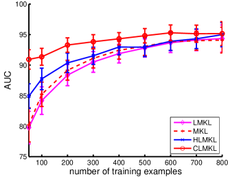
(a) Splice

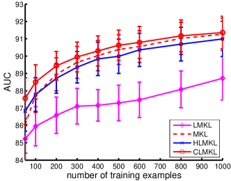
(b) TSS

Figure 1: Results of the gene finding experiments: splice site detection (left) and transcription start site detection (right). To clean the presentation, results for UNIF are not given here. The parameter $p$ for CLMKL, HLMKL and MKL is set as $1$ here.

We observe that CLMKL achieves, for all $n$, a significant gain over all baselines. This improvement is especially strong for small $n$. For $n=50$, CLMKL attains $90.9\%$ accuracy, while the best baseline only achieves $85.4\%$, improving by $5.5\%$. Detailed results with standard deviation are reported in Table 1. A hypothetical explanation of the improvement from CLMKL is that splice sites are characterized by nucleotide sequences—so-called motifs—the length of which may differ from site to site [47]. The 20 employed kernels count matching subsequences of length 1 to 20, respectively. For sites characterized by smaller motifs, low-degree WD-kernels are thus more effective than high-degree ones, and vice versa for sites containing longer motifs.

	$50$	$100$	$200$	$300$	$400$	$500$	$600$	$700$	$800$
UNIF	$79.5\!\pm\!2.8\bullet$	$84.2\!\pm\!2.2\bullet$	$88.0\!\pm\!1.7\bullet$	$90.0\!\pm\!1.7\bullet$	$91.6\!\pm\!1.5\bullet$	$92.4\!\pm\!1.5\bullet$	$93.3\!\pm\!1.7\bullet$	$93.6\!\pm\!1.7\bullet$	$93.8\!\pm\!2.3\bullet$
LMKL	$79.8\!\pm\!2.7\bullet$	$84.2\!\pm\!2.3\bullet$	$88.4\!\pm\!1.7\bullet$	$90.5\!\pm\!1.7\bullet$	$91.9\!\pm\!1.5\bullet$	$92.8\!\pm\!1.5\bullet$	$93.7\!\pm\!1.6\bullet$	$94.1\!\pm\!1.7\bullet$	$94.3\!\pm\!2.2\bullet$
MKL,p=1	$80.2\!\pm\!2.8\bullet$	$85.2\!\pm\!2.0\bullet$	$89.2\!\pm\!1.6\bullet$	$91.1\!\pm\!1.6\bullet$	$92.5\!\pm\!1.5\bullet$	$93.1\!\pm\!1.5\bullet$	$93.9\!\pm\!1.4\bullet$	$94.0\!\pm\!1.6\bullet$	$94.2\!\pm\!2.1\bullet$
MKL,p=2	$79.6\!\pm\!2.8\bullet$	$84.3\!\pm\!2.2\bullet$	$88.3\!\pm\!1.7\bullet$	$90.4\!\pm\!1.6\bullet$	$91.8\!\pm\!1.5\bullet$	$92.5\!\pm\!1.5\bullet$	$93.4\!\pm\!1.6\bullet$	$93.6\!\pm\!1.6\bullet$	$93.8\!\pm\!2.2\bullet$
MKL,p=1.33	$79.7\!\pm\!2.9\bullet$	$84.6\!\pm\!2.1\bullet$	$88.6\!\pm\!1.7\bullet$	$90.6\!\pm\!1.6\bullet$	$92.0\!\pm\!1.5\bullet$	$92.7\!\pm\!1.5\bullet$	$93.5\!\pm\!1.5\bullet$	$93.7\!\pm\!1.6\bullet$	$93.8\!\pm\!2.1\bullet$
HLMKL,p=1	$84.9\!\pm\!2.0\bullet$	$87.7\!\pm\!1.8\bullet$	$90.4\!\pm\!1.6\bullet$	$91.5\!\pm\!1.4\bullet$	$93.0\!\pm\!1.3\bullet$	$92.9\!\pm\!1.6\bullet$	$93.9\!\pm\!1.5\bullet$	$94.3\!\pm\!1.6\bullet$	$95.0\!\pm\!2.0\bullet$
HLMKL,p=2	$84.9\!\pm\!2.0\bullet$	$87.0\!\pm\!1.7\bullet$	$90.4\!\pm\!1.4\bullet$	$91.1\!\pm\!1.6\bullet$	$92.6\!\pm\!1.4\bullet$	$93.5\!\pm\!1.6\bullet$	$94.7\!\pm\!1.4\bullet$	$94.6\!\pm\!1.4\bullet$	$94.4\!\pm\!2.2\bullet$
HLMKL,p=1.33	$85.4\!\pm\!1.9\bullet$	$88.5\!\pm\!1.7\bullet$	$90.1\!\pm\!1.6\bullet$	$91.7\!\pm\!1.4\bullet$	$92.7\!\pm\!1.2\bullet$	$93.4\!\pm\!1.6\bullet$	$94.6\!\pm\!1.5\bullet$	$94.4\!\pm\!1.7\bullet$	$94.4\!\pm\!2.1\bullet$
CLMKL,p=1	$90.9\!\pm\!1.6$	$91.3\!\pm\!1.4\bullet$	$93.3\!\pm\!1.2\bullet$	$93.8\!\pm\!1.2\bullet$	$94.3\!\pm\!1.0\bullet$	$94.8\!\pm\!1.2$	$95.3\!\pm\!1.3\bullet$	$95.1\!\pm\!1.4\bullet$	$95.2\!\pm\!2.0\bullet$
CLMKL,p=2	$90.5\!\pm\!1.6\bullet$	$92.3\!\pm\!1.2\bullet$	$93.0\!\pm\!1.2\bullet$	$94.0\!\pm\!1.2$	$94.4\!\pm\!1.1\bullet$	$94.7\!\pm\!1.2\bullet$	$95.4\!\pm\!1.4\bullet$	$95.3\!\pm\!1.5\bullet$	$95.6\!\pm\!1.9\bullet$
CLMKL,p=1.33	$90.9\!\pm\!1.5$	$90.1\!\pm\!1.3$	$92.7\!\pm\!1.2$	$94.1\!\pm\!1.2$	$94.8\!\pm\!1.1$	$94.9\!\pm\!1.1$	$95.6\!\pm\!1.2$	$95.4\!\pm\!1.5$	$95.4\!\pm\!1.9$

Table 1: Performances achieved by LMKL, UNIF, regular $\ell_{p}$ MKL, HLMKL, and CLMKL on Splice Dataset. $\bullet$ indicates that CLMKL with $p=1.33$ is significantly better than the compared method (paired t-tests at $95\%$ significance level).

5.3 Transcription Start Site Detection

Our next experiment aims at detecting transcription start sites (TSS) of RNA Polymerase II binding genes in genomic DNA sequences. We experiment on the TSS data set, which we downloaded from http://mldata.org/repository/data/viewslug/tss/. This data set, which is included in the larger study of [46], comes with $5$ kernels. The SVM based on the uniform combination of these $5$ kernels was found to have the highest overall performance among $19$ promoter prediction programs [1]. It therefore constitutes a strong baseline. To be consistent with previous studies [1, 24, 46], we use the area under the ROC curve (AUC) as an evaluation criterion. We consider the same experimental setup as in the splice detection experiment. The gating function and the partition are computed with the TSS kernel, which carries most of the discriminative information [46]. All kernel matrices were normalized with respect to their trace, prior to the experiment.

	$50$	$100$	$200$	$300$	$400$	$500$	$600$	$800$	$1000$
UNIF	$83.9\!\pm\!2.4\bullet$	$86.2\!\pm\!1.3\bullet$	$87.6\!\pm\!1.0\bullet$	$88.4\!\pm\!0.9\bullet$	$88.7\!\pm\!0.9\bullet$	$89.1\!\pm\!0.9\bullet$	$89.2\!\pm\!1.0\bullet$	$89.6\!\pm\!1.1\bullet$	$89.8\!\pm\!1.1\bullet$
LMKL	$85.2\!\pm\!1.2\bullet$	$85.9\!\pm\!1.1\bullet$	$86.6\!\pm\!1.1\bullet$	$87.1\!\pm\!1.0\bullet$	$87.2\!\pm\!0.9\bullet$	$87.3\!\pm\!1.0\bullet$	$87.5\!\pm\!1.0\bullet$	$88.1\!\pm\!1.1\bullet$	$88.7\!\pm\!1.3\bullet$
MKL,p=1	$86.0\!\pm\!1.7\bullet$	$87.7\!\pm\!1.0\bullet$	$88.9\!\pm\!0.9\bullet$	$89.6\!\pm\!0.9\bullet$	$90.0\!\pm\!0.9\bullet$	$90.3\!\pm\!0.9\bullet$	$90.5\!\pm\!0.9$	$91.0\!\pm\!0.9$	$91.2\!\pm\!0.9$
MKL,p=2	$85.1\!\pm\!2.0\bullet$	$86.9\!\pm\!1.1\bullet$	$88.1\!\pm\!0.9\bullet$	$88.8\!\pm\!0.9\bullet$	$89.2\!\pm\!0.9\bullet$	$89.6\!\pm\!0.9\bullet$	$89.8\!\pm\!1.0\bullet$	$90.3\!\pm\!1.0\bullet$	$90.7\!\pm\!0.9\bullet$
MKL,p=1.33	$85.7\!\pm\!1.8\bullet$	$87.5\!\pm\!1.0\bullet$	$88.7\!\pm\!0.9\bullet$	$89.4\!\pm\!0.9\bullet$	$89.8\!\pm\!0.9\bullet$	$90.2\!\pm\!0.9\bullet$	$90.4\!\pm\!0.9\bullet$	$90.9\!\pm\!0.9\bullet$	$91.2\!\pm\!0.9\bullet$
HLMKL,p=1	$86.8\!\pm\!1.2\bullet$	$87.8\!\pm\!1.0\bullet$	$88.7\!\pm\!0.9\bullet$	$89.4\!\pm\!0.9\bullet$	$89.8\!\pm\!1.0\bullet$	$90.0\!\pm\!1.0\bullet$	$90.4\!\pm\!1.0\bullet$	$90.7\!\pm\!1.0\bullet$	$91.0\!\pm\!1.0\bullet$
HLMKL,p=2	$86.3\!\pm\!1.4\bullet$	$87.5\!\pm\!1.0\bullet$	$88.5\!\pm\!0.9\bullet$	$89.3\!\pm\!0.9\bullet$	$89.4\!\pm\!0.9\bullet$	$89.7\!\pm\!0.9\bullet$	$89.8\!\pm\!1.0\bullet$	$90.3\!\pm\!1.1\bullet$	$90.5\!\pm\!1.0\bullet$
HLMKL,p=1.33	$86.5\!\pm\!1.4\bullet$	$87.7\!\pm\!1.1\bullet$	$88.7\!\pm\!0.9\bullet$	$89.3\!\pm\!0.9\bullet$	$89.8\!\pm\!1.0\bullet$	$90.1\!\pm\!0.9\bullet$	$90.2\!\pm\!1.0\bullet$	$90.7\!\pm\!1.0\bullet$	$91.0\!\pm\!0.9\bullet$
CLMKL,p=1	$87.6\!\pm\!1.2$	$88.5\!\pm\!1.0$	$89.4\!\pm\!0.8$	$90.0\!\pm\!0.9$	$90.3\!\pm\!0.9\bullet$	$90.6\!\pm\!0.9$	$90.8\!\pm\!0.9\bullet$	$91.2\!\pm\!0.9\bullet$	$91.4\!\pm\!0.9$
CLMKL,p=2	$87.3\!\pm\!1.3\bullet$	$88.3\!\pm\!1.0\bullet$	$89.1\!\pm\!0.8\bullet$	$89.6\!\pm\!0.8\bullet$	$89.9\!\pm\!0.9\bullet$	$90.2\!\pm\!0.9\bullet$	$90.3\!\pm\!0.9\bullet$	$90.7\!\pm\!1.0\bullet$	$90.9\!\pm\!0.9\bullet$
CLMKL,p=1.33	$87.6\!\pm\!1.2$	$88.6\!\pm\!0.9$	$89.4\!\pm\!0.8$	$89.9\!\pm\!0.9$	$90.2\!\pm\!0.9$	$90.5\!\pm\!0.9$	$90.6\!\pm\!1.0$	$91.1\!\pm\!1.0$	$91.3\!\pm\!0.9$

Table 2: Performances achieved by LMKL, UNIF, regular $\ell_{p}$ MKL, HLMKL and CLMKL on TSS Dataset. $\bullet$ indicates that CLMKL with $p=1.33$ is significantly better than the compared method (paired t-tests at $95\%$ significance level).

Figure 1 (b) shows the AUCs on the test data sets as a function of the number of training examples.We observe that CLMKL attains a consistent improvement over other competing methods. Again, this improvement is most significant when $n$ is small. Detailed results with standard deviation are reported in Table 2.

5.4 Protein Fold Prediction

	UNIF	LMKL	MKL			HLMKL			CLMKL
			$p=1$	$p=1.2$	$p=2$	$p=1$	$p=1.2$	$p=2$	$p=1$	$p=1.2$	$p=2$
ACC	$68.4\bullet$	$64.3\bullet$	$68.7\bullet$	$74.2\bullet$	$70.8\bullet$	$72.7\pm 1.3\bullet$	$74.6\pm 0.6$	$72.4\pm 0.8\bullet$	$71.3\pm 0.5\bullet$	$\bm{75.0\pm 0.7}$	$71.7\pm 0.5\bullet$

Table 3: Results of the protein fold prediction experiment. $\bullet$ indicates that CLMKL with $p=1.2$ is significantly better than the compared method (paired t-tests at $95\%$ significance level).

Protein fold prediction is a key step towards understanding the function of proteins, as the folding class of a protein is closely linked with its function; thus it is crucial for drug design. We experiment on the protein folding class prediction dataset by Ding and Dubchak [13], which was also used in Campbell and Ying [7], Kloft [24], Kloft and Blanchard [25]. This dataset consists of $27$ fold classes with $311$ proteins used for training and $383$ proteins for testing. We use exactly the same $12$ kernels as in Campbell and Ying [7], Kloft [24], Kloft and Blanchard [25] reflecting different features, such as van der Waals volume, polarity and hydrophobicity. We precisely replicate the experimental setup of previous experiments by Campbell and Ying [7], Kloft [24], Kloft and Blanchard [25], which is detailed in Supplementary Material E.1. We report the mean prediction accuracies, as well as standard deviations in Table 3.

The results show that CLMKL surpasses regular $\ell_{p}$-norm MKL for all values of $p$, and achieves accuracies up to $0.6\%$ higher than the one reported in Kloft [24], which is higher than the initially reported accuracies in Campbell and Ying [7]. LMKL works poorly in this dataset, possibly because LMKL based on precomputed custom kernels requires to optimize $nM$ additional variables, which may overfit.

5.5 Visual Image Categorization—UIUC Sports

We experiment on the UIUC Sports event dataset [35] consisting of 1574 images, belonging to 8 image classes of sports activities. We compute 9 $\chi^{2}$-kernels based on SIFT features and global color histograms, which is described in detail in Supplemental Material E.2, where we also give background on the experimental setup.

From the results shown in Table 4, we observe that CLMKL achieves a performance improvement by $0.26\%$ over the $\ell_{p}$-norm MKL baseline while localized MKL as in Gönen and Alpaydin [14] underperforms the MKL baseline.

	MKL	LMKL	CLMKL		MKL	LMKL	CLMKL
ACC	90.00	87.29	90.26	$\Delta$	0+ 11= 0-	0+ 1= 10-	4+ 6= 1-

Table 4: Results of the visual image recognition experiment on the UIUC sports dataset. $\Delta$ indicates on how many outer cross validation test splits a method is worse ($n-$), equal ($n=$) or better ($n+$) than MKL.

5.6 Execution Time Experiments

To demonstrate the efficiency of the proposed implementation, we compare the training time for UNIF, LMKL, $\ell_{p}$-norm MKL, HLMKL and CLMKL on the TSS dataset. We fix the regularization parameter

$C=1$. We fix $l=3$ and $\text{AE}=0.5$ for CLMKL, and fix $l=3$ for HLMKL. On the image to the right, we plot the training time versus the training set size. We repeat the experiment $20$ times and report the average training time here. We optimize CLMKL, HLMKL and MKL until the relative gap is under $10^{-3}$. The figure implies that CLMKL converges faster than LMKL. Furthermore, training an $\ell_{2}$-norm MKL requires significantly less time than training an $\ell_{1}$-norm MKL, which is consistent with the fact that the dual problem of $\ell_{2}$-norm MKL is much smoother than the $\ell_{1}$-norm counterpart.

6 Conclusions

Localized approaches to multiple kernel learning allow for flexible distribution of kernel weights over the input space, which can be a great advantage when samples require varying kernel importance. As we show in this paper, this can be the case in image recognition and several computational biology applications. However, almost prevalent approaches to localized MKL require solving difficult non-convex optimization problems, which makes them potentially prone to overfitting as theoretical guarantees such as generalization error bounds are yet unknown.

In this paper, we propose a theoretically grounded approach to localized MKL, consisting of two subsequent steps: 1. clustering the training instances and 2. computation of the kernel weights for each cluster through a single convex optimization problem. For which we derive an efficient optimization algorithm based on Fenchel duality. Using Rademacher complexity theory, we establish large-deviation inequalities for localized MKL, showing that the smoothness in the cluster membership assignments crucially controls the generalization error. The proposed method is well suited for deployment in the domains of computer vision and computational biology. For splice site detection, CLMKL achieves up to $5\%$ higher accuracy than its global and non-convex localized counterparts.

Future work could analyze extension of the methodology to semi-supervised learning [17, 18] or using different clustering objectives [52, 21] and how to principally include the construction of the data partition into our framework by constructing partitions that can capture the local variation of prediction importance of different features.

Supplemental Material

Appendix A Lemmata and Proofs

A.1 Lemmata Used for Dualization in Section 2.3

Let $H_{1},\ldots,H_{M}$ be $M$ Hilbert spaces and $p\geq 1$. Define the function $g_{p}(v_{1},\ldots,v_{M}):H_{1}\times\cdots\times H_{M}\to\mathbb{R}$ by

$$g_{p}(v_{1},\ldots,v_{M})=\frac{1}{2}\|(v_{1},\ldots,v_{M})\|^{2}_{2,p},\quad p\geq 1.$$

For any $p\geq 1$, denote by $p^{*}$ the conjugated exponent satisfying $\frac{1}{p}+\frac{1}{p^{*}}=1$.

Lemma A.1.

The gradient of $g_{p}$ is

$$\frac{\partial g_{p}(v_{1},\ldots,v_{M})}{\partial v_{m}}=\big{[}\sum_{\tilde{m}\in\mathbb{N}_{M}}\|v_{\tilde{m}}\|_{2}^{p}\big{]}^{\frac{2}{p}-1}\|v_{m}\|_{2}^{p-2}v_{m}.$$

Proof.

By the chain rule, we have

$$\frac{\partial g_{p}(v_{1},\ldots,v_{M})}{\partial v_{m}} =\frac{1}{p}\big{[}\sum_{\tilde{m}\in\mathbb{N}_{M}}\|v_{\tilde{m}}\|_{2}^{p}\big{]}^{\frac{2}{p}-1}\frac{\partial\langle v_{m},v_{m}\rangle^{\frac{p}{2}}}{\partial v_{m}}$$

$$=\frac{1}{2}\big{[}\sum_{\tilde{m}\in\mathbb{N}_{M}}\|v_{\tilde{m}}\|_{2}^{p}\big{]}^{\frac{2}{p}-1}\frac{\partial\langle v_{m},v_{m}\rangle}{\partial v_{m}}\langle v_{m},v_{m}\rangle^{\frac{p}{2}-1}$$

$$=\big{[}\sum_{\tilde{m}\in\mathbb{N}_{M}}\|v_{\tilde{m}}\|_{2}^{p}\big{]}^{\frac{2}{p}-1}\|v_{m}\|_{2}^{p-2}v_{m}.$$

∎

Lemma A.2 (Micchelli and Pontil 40).

Let $a_{i}\geq 0,i\in\mathbb{N}_{d}$ and $1\leq r<\infty$. Then

$$\min_{\eta:\eta_{i}\geq 0,\sum_{i\in\mathbb{N}_{d}}\eta_{i}^{r}\leq 1}\sum_{i\in\mathbb{N}_{d}}\frac{a_{i}}{\eta_{i}}=\Big{(}\sum_{i\in\mathbb{N}_{d}}a_{i}^{\frac{r}{r+1}}\Big{)}^{1+\frac{1}{r}}$$

and the minimum is attained at $\eta_{i}=a_{i}^{\frac{1}{r+1}}\Big{(}\sum_{k\in\mathbb{N}_{d}}a_{k}^{\frac{r}{r+1}}\Big{)}^{-\frac{1}{r}}.$

A.2 Proof of Representer Theorem (Theorem 3)

Proof of Theorem 3.

In our derivation (2.3) of the dual problem, the variable $w_{j}(\alpha):=\big{(}w_{j}^{(1)}(\alpha),\ldots,w_{j}^{(M)}(\alpha)\big{)}$ should meet the optimality in the sense

$$w_{j}(\alpha)=\arg\max_{v_{1}\in H_{1},\ldots,v_{M}\in H_{M}}\bigg{[}\Big{\langle}(v_{m})_{m=1}^{M},\Big{(}\sum_{i=1}^{n}\alpha_{i}c_{j}(x_{i})\phi_{m}(x_{i})\Big{)}_{m=1}^{M}\Big{\rangle}-\frac{1}{2}\|(v_{m})_{m=1}^{M}\|^{2}_{2,\frac{2p}{p+1}}\bigg{]}.$$

Since $(\bigtriangledown f)^{-1}=\bigtriangledown f^{*}$ for any convex function $f$ and the Fenchel-conjugate of $g_{p}$ is $g_{p^{*}}$, we obtain

$$w_{j}(\alpha) =\bigtriangledown g^{-1}_{\frac{2p}{p+1}}\Big{(}\sum_{i\in\mathbb{N}_{n}}\alpha_{i}c_{j}(x_{i})\phi_{1}(x_{i}),\ldots,\sum_{i\in\mathbb{N}_{n}}\alpha_{i}c_{j}(x_{i})\phi_{M}(x_{i})\Big{)}$$

$$=\bigtriangledown g_{\frac{2p}{p-1}}\Big{(}\sum_{i\in\mathbb{N}_{n}}\alpha_{i}c_{j}(x_{i})\phi_{1}(x_{i}),\ldots,\sum_{i\in\mathbb{N}_{n}}\alpha_{i}c_{j}(x_{i})\phi_{M}(x_{i})\Big{)}$$

$$\stackrel{{\scriptstyle\text{Lem.~{}\ref{lem:gradient-pnorm}}}}{{=}}\big{[}\sum_{\tilde{m}\in\mathbb{N}_{M}}\|\sum_{i\in\mathbb{N}_{n}}\alpha_{i}c_{j}(x_{i})\phi_{\tilde{m}}(x_{i})\|_{2}^{\frac{2p}{p-1}}\big{]}^{-\frac{1}{p}}\Big{(}\big{\|}\sum_{i\in\mathbb{N}_{n}}\alpha_{i}c_{j}(x_{i})\phi_{1}(x_{i})\big{\|}_{2}^{\frac{2}{p-1}}\big{[}\sum_{i\in\mathbb{N}_{n}}\alpha_{i}c_{j}(x_{i})\phi_{1}(x_{i})\big{]},$$

$$\qquad\ldots,\big{\|}\sum_{i\in\mathbb{N}_{n}}\alpha_{i}c_{j}(x_{i})\phi_{M}(x_{i})\big{\|}_{2}^{\frac{2}{p-1}}\big{[}\sum_{i\in\mathbb{N}_{n}}\alpha_{i}c_{j}(x_{i})\phi_{M}(x_{i})\big{]}\Big{)}.$$

Note that the above derivation uses Lemma A.1 from Supplemental Material A.1. ∎

A.3 Proof of Proposition 5

Proof of Proposition 5.

Fixing the variables $w_{j}^{(m)}$ and $b$, the optimization problem (P) reduces to

$$\min_{\beta}\;\sum_{j\in\mathbb{N}_{l}}\sum_{m\in\mathbb{N}_{M}}\frac{\|w_{j}^{(m)}\|_{2}^{2}}{2\beta_{jm}}\quad\mbox{s.t.}\;\sum_{m\in\mathbb{N}_{M}}\beta^{p}_{jm}\leq 1,\beta_{jm}\geq 0,\;\forall j\in\mathbb{N}_{l},m\in\mathbb{N}_{M}.$$

This problem can be decomposed into $l$ independent subproblems, one at each locality. For example, the subproblem at the $j$-th locality is as follows

$$\min_{\beta}\;\sum_{m\in\mathbb{N}_{M}}\frac{\|w_{j}^{(m)}\|_{2}^{2}}{2\beta_{jm}}\quad\mbox{s.t.}\;\sum_{m\in\mathbb{N}_{M}}\beta^{p}_{jm}\leq 1,\beta_{jm}\geq 0,\;\forall m\in\mathbb{N}_{M}.$$

Applying Lemma A.2 with $\alpha_{m}=\|w_{j}^{(m)}\|_{2}^{2}$, $\eta_{m}=\beta_{jm}$ and $r=p$ completes the proof. ∎

A.4 Proof of Theorem 6: Convergence of the CLMKL Optimization Algorithm

The following lemma is a direct consequence of Lemma 3.1 and Theorem 4.1 in Tseng [50].

Lemma A.3.

Let $f:\mathbb{R}^{d_{1}+\cdots+d_{R}}\to\mathbb{R}\cup\{\infty\}$ be a function. Put $d=d_{1}+\cdots+d_{R}$. Suppose that $f$ can be decomposed into $f(\alpha_{1},\ldots,\alpha_{R})+\sum_{r\in\mathbb{N}_{R}}f_{r}(\alpha_{r})$ for some $f_{0}:\mathbb{R}^{d}\to\mathbb{R}\cup\{\infty\}$ and $f_{r}:\mathbb{R}^{d_{r}}\to\mathbb{R}\cup\{\infty\},r\in\mathbb{N}_{R}$. Initialize the block coordinate descent method by $\alpha^{0}=(\alpha^{0}_{1},\ldots,\alpha_{R}^{0})$. Define the iterates $\alpha^{k}=(\alpha_{1}^{k},\ldots,\alpha_{R}^{k})$ by

$$\alpha_{r}^{k+1}=\arg\min_{\mathfrak{u}\in\mathbb{R}^{d_{k}}}f(\alpha_{1}^{k+1},\ldots,\alpha_{r-1}^{k+1},\mathfrak{u},\alpha^{k}_{r+1},\ldots,\alpha^{k}_{R}),\quad\forall r\in\mathbb{N}_{R},k\in\mathbb{N}_{+}.$$ (A.1)

Assume that

1. $f$ is convex and proper, i.e., $f\not\equiv\infty$

2. the sublevel set $\mathcal{A}^{0}:=\{\alpha\in\mathbb{R}^{d}:f(\alpha)\leq f(\alpha^{0})\}$ is compact and $f$ is continuous on $\mathcal{A}^{0}$

3. $\text{dom}(f_{0}):=\{\alpha\in\mathbb{R}^{d}:f_{0}(\alpha)\leq\infty\}$ is open and $f_{0}$ is continuously differentiable on $\text{dom}(f_{0})$.

Then, the minimizer in (A.1) exists and any limit point of the sequence $(\alpha^{k})_{k\in\mathbb{N}_{+}}$ minimizes $f$ over $\mathcal{A}^{0}$.

The proof of Theorem 6 is a direct consequence of the above lemma.

Proof of Theorem 6.

The primal problem (P) can be rewritten as follows:

$$\inf_{w,\beta_{j}\in\Theta_{p},j\in\mathbb{N}_{l}}\sum_{j\in\mathbb{N}_{l}}\sum_{m\in\mathbb{N}_{M}}\frac{\|w_{j}^{(m)}\|_{2}^{2}}{2\beta_{jm}}+C\sum_{i\in\mathbb{N}_{n}}\ell(\sum_{j\in\mathbb{N}_{l}}c_{j}(x_{i})\sum_{m\in\mathbb{N}_{M}}\langle w_{j}^{(m)},\phi_{m}(x_{i})\rangle,y_{i}),$$ (A.2)

where $\Theta_{p}=\{(\theta_{1},\ldots,\theta_{M})\in\mathbb{R}^{M}:\theta_{m}\geq 0,\|(\theta_{m})_{m=1}^{M}\|_{p}\leq 1\}$, and $w_{j}^{(m)}\in\mathbb{R}^{e_{m}},\forall j\in\mathbb{N}_{l},m\in\mathbb{N}_{M}$. Note that Eq. (A.2) can be written as the following unconstrained problem:

$$\inf_{w,\beta}f(w,\beta),\qquad\text{where }f(w,\beta)=f_{0}(w,\beta)+f_{1}(w)+f_{2}(\beta),$$

with

$$f_{0}(w,\beta)=\sum_{j\in\mathbb{N}_{l}}\sum_{m\in\mathbb{N}_{M}}\Big{[}\frac{\|w_{j}^{(m)}\|_{2}^{2}}{2\beta_{jm}}+I_{\beta_{jm}\geq 0}(\beta_{jm})\Big{]}$$

$$f_{1}(w)=C\sum_{i\in\mathbb{N}_{n}}\ell(\sum_{j\in\mathbb{N}_{l}}c_{j}(x_{i})\sum_{m\in\mathbb{N}_{M}}\langle w_{j}^{(m)},\phi_{m}(x_{i})\rangle,y_{i})\quad\text{and }f_{2}(\beta)=\sum_{j\in\mathbb{N}_{l}}I_{\|\beta_{j}\|_{p}\leq 1}(\beta_{j}).$$

Here $I$ is the indicator function, i.e., $I_{S}(s)=0$ if $s\in S$ and $\infty$ otherwise.

Now, it remains to check the assumption (A1), (A2) and (A3) in Lemma A.3 for Algorithm 1.

Validity of A1. It is known that a quadratic over a linear function is convex, so the term $\sum_{j\in\mathbb{N}_{l}}\sum_{m\in\mathbb{N}_{M}}\frac{\|w_{j}^{(m)}\|_{2}^{2}}{2\beta_{jm}}$ is convex. Also, since $\ell$ is convex w.r.t. the first argument and the term $\sum_{j\in\mathbb{N}_{l}}c_{j}(x_{i})\sum_{m\in\mathbb{N}_{M}}\langle w_{j}^{(m)},\phi_{m}(x_{i})\rangle$ is a linear function of $w$, we immediately know the term $\sum_{i\in\mathbb{N}_{n}}\ell(\sum_{j\in\mathbb{N}_{l}}c_{j}(x_{i})\sum_{m\in\mathbb{N}_{M}}\langle w_{j}^{(m)},\phi_{m}(x_{i})\rangle,y_{i})$ is convex. The convexity of $f$ follows immediately. For the initial assignment $w^{(0)}=\{w_{j}^{(m,0)}\}_{j,m}$ with $w_{j}^{(m,0)}=0$ and $\beta^{(0)}=\{\beta^{(0)}_{jm}\}_{jm}$ with $\beta^{(0)}_{jm}=M^{-1/p}$, we know

$$f(w^{(0)},\beta^{(0)})=Cn\sup_{y\in\mathcal{Y}}\ell(0,y)<\infty$$

and therefore $f$ is proper.

Validity of A2. Recall that our algorithm is initialized with $w^{(0)}=0$ and $\beta^{(0)}=M^{-1/p}$. For any $(w,\beta)\in\mathcal{A}^{0}:=\{(\bar{w},\bar{\beta}):f(\bar{w},\bar{\beta})\leq Cn\sup_{y\in\mathcal{Y}}\ell(0,y)\}$, we have

$$\|w_{j}^{(m)}\|^{2}_{2}\leq 2\beta_{jm}Cn\sup_{y\in\mathcal{Y}}\ell(0,y)\leq 2Cn\sup_{y\in\mathcal{Y}}\ell(0,y),$$

which, coupled with the constraint $\|(\beta_{jm})_{m=1}^{M}\|_{p}\leq 1,\forall j\in\mathbb{N}_{l}$, immediately shows that $\mathcal{A}^{0}$ is bounded. Furthermore, since $f_{0},f_{1}$ and $f_{2}$ are continuous on their respective domains, the function $f$ is therefore continuous on $\mathcal{A}^{0}\subset\text{dom}(f_{0})\cap\text{dom}(f_{1})\cap\text{dom}(f_{2})$. It is also known that the preimage of a closed set is closed under a continuous function, from which we know the set $\mathcal{A}^{0}=f^{-1}(-\infty,f(w^{(0)},\beta^{(0)})]$ is closed. Any closed and bounded subset in $\mathbb{R}^{d},d\in\mathbb{N}$ is compact and thus $\mathcal{A}^{(0)}$ is compact.

Validity of A3. Clearly, $\text{dom}(f_{0})=\{(w,\beta):\beta>0\}$ is open and $f_{0}$ is continuously differentiable on $\text{dom}(f_{0})$. ∎

A.5 Proof of Generalization Error Bounds (Theorem 8)

In this section we present the proof of the achieved generalization error bounds (Theorem 9 in the main text). Denote $\bar{p}=\frac{2p}{p+1}$ for any $p\geq 1$ and observe that $\bar{p}\leq 2$, which implies $\bar{p}^{*}\geq 2$. To start with, we give a discussion on the interpretation and tightness of Rademacher complexity bounds in Theorem 8.

Interpretation and Tightness of Rademacher complexity bounds

It can be directly checked that the function $x\to xM^{2/x}$ is decreasing along the interval $(0,2\log M)$ and increasing along the interval $(2\log M,\infty)$. Therefore, under the assumption $k_{m}(x,x)\leq B$ the Rademacher complexity bounds thus satisfy the inequalities:

$$\hat{R}_{n}(H_{p,D})\leq\sqrt{\frac{DB}{n}}\times\begin{cases}\frac{1}{n}\sqrt{2eDB\log M[\sum_{j\in\mathbb{N}_{l}}\sum_{i\in\mathbb{N}_{n}}c_{j}^{2}(x_{i})]},&\text{if }p\leq\frac{\log M}{\log M-1},\\ \frac{1}{n}\sqrt{\frac{2p}{p-1}DBM^{\frac{p-1}{p}}[\sum_{j\in\mathbb{N}_{l}}\sum_{i\in\mathbb{N}_{n}}c_{j}^{2}(x_{i})]},&\text{otherwise}.\end{cases}$$

In particular, the former expression can be taken for $p=1$, resulting in a mild logarithmic dependence on the number of kernels. Note that in the limiting case of just one cluster, i.e., $l=1$, the Rademacher complexity bounds match the result by Cortes et al. [10], which was shown to be tight.

The proof of Theorem 8 is based on the following lemmata.

Lemma A.4 (Khintchine-Kahane inequality [23]).

Let $v_{1},\ldots,v_{n}\in\mathcal{H}$. Then, for any $q\geq 1$, it holds

$$\mathbb{E}_{\bm{\sigma}}\big{\|}\sum_{i\in\mathbb{N}_{n}}\sigma_{i}v_{i}\big{\|}_{2}^{q}\leq\bigg{(}q\sum_{i\in\mathbb{N}_{n}}\|v_{i}\|_{2}^{2}\bigg{)}^{\frac{q}{2}}.$$

Lemma A.5 (Block-structured Hölder inequality [26]).

Let $x=(x^{(1)},\ldots,x^{(n)}),y=(y^{(1)},\ldots,y^{(n)})\in\mathcal{H}=\mathcal{H}_{1}\times\cdots\times\mathcal{H}_{n}$. Then, for any $p\geq 1$, it holds

$$\langle x,y\rangle\leq\|x\|_{2,p}\|y\|_{2,p^{*}}.$$

Proof of Theorem 8.

Firstly, for any $1\leq\bar{t}\leq 2$ we can apply a block-structured version of Hölder inequality to bound $\sum_{i\in\mathbb{N}_{n}}\sigma_{i}f_{w}(x_{i})$ by

$$\begin{split}\sum_{i\in\mathbb{N}_{n}}\sigma_{i}f_{w}(x_{i})&=\sum_{i\in\mathbb{N}_{n}}\sigma_{i}\Big{[}\sum_{j\in\mathbb{N}_{l}}c_{j}(x_{i})\sum_{m\in\mathbb{N}_{M}}\langle w_{j}^{(m)},\phi_{m}(x_{i})\rangle\Big{]}\\ &=\sum_{i\in\mathbb{N}_{n}}\sigma_{i}\Big{[}\sum_{j\in\mathbb{N}_{l}}c_{j}(x_{i})\langle w_{j},\phi(x_{i})\rangle\Big{]}\\ &=\sum_{j\in\mathbb{N}_{l}}\bigg{\langle}w_{j},\sum_{i\in\mathbb{N}_{n}}\sigma_{i}c_{j}(x_{i})\phi(x_{i})\bigg{\rangle}\\ &\stackrel{{\scriptstyle\text{H\"{o}lder}}}{{\leq}}\sum_{j\in\mathbb{N}_{l}}\Big{[}\|w_{j}\|_{2,\bar{t}}\Big{\|}\sum_{i\in\mathbb{N}_{n}}\sigma_{i}c_{j}(x_{i})\phi(x_{i})\Big{\|}_{2,\bar{t}^{*}}\Big{]}\\ &\stackrel{{\scriptstyle\text{C.~{}S}}}{{\leq}}\Big{[}\sum_{j\in\mathbb{N}_{l}}\|w_{j}\|^{2}_{2,\bar{t}}\Big{]}^{\frac{1}{2}}\Big{[}\sum_{j\in\mathbb{N}_{l}}\Big{\|}\sum_{i\in\mathbb{N}_{n}}\sigma_{i}c_{j}(x_{i})\phi(x_{i})\Big{\|}^{2}_{2,\bar{t}^{*}}\Big{]}^{\frac{1}{2}}.\end{split}$$ (A.3)

For any $j\in\mathbb{N}_{l}$, the Khintchine-Kahane (K.-K.) inequality and Jensen inequality (since $\bar{t}^{*}\geq 2$) permit us to bound $\mathbb{E}_{\bm{\sigma}}\Big{\|}\sum_{i\in\mathbb{N}_{n}}\sigma_{i}c_{j}(x_{i})\phi(x_{i})\Big{\|}^{2}_{2,\bar{t}^{*}}$ by

$$\mathbb{E}_{\bm{\sigma}}\Big{\|}\sum_{i\in\mathbb{N}_{n}}\sigma_{i}c_{j}(x_{i})\phi(x_{i})\Big{\|}^{2}_{2,\bar{t}^{*}} \stackrel{{\scriptstyle\text{def}}}{{=}}\mathbb{E}_{\bm{\sigma}}\bigg{[}\sum_{m\in\mathbb{N}_{M}}\Big{\|}\sum_{i\in\mathbb{N}_{n}}\sigma_{i}c_{j}(x_{i})\phi_{m}(x_{i})\Big{\|}_{2}^{\bar{t}^{*}}\bigg{]}^{\frac{2}{\bar{t}^{*}}}$$

$$\stackrel{{\scriptstyle\text{Jensen}}}{{\leq}}\bigg{[}\mathbb{E}_{\bm{\sigma}}\sum_{m\in\mathbb{N}_{M}}\Big{\|}\sum_{i\in\mathbb{N}_{n}}\sigma_{i}c_{j}(x_{i})\phi_{m}(x_{i})\Big{\|}_{2}^{\bar{t}^{*}}\bigg{]}^{\frac{2}{\bar{t}^{*}}}$$

$$\stackrel{{\scriptstyle\text{K.-K.}}}{{\leq}}\bigg{[}\sum_{m\in\mathbb{N}_{M}}\Big{(}\bar{t}^{*}\sum_{i\in\mathbb{N}_{n}}c_{j}^{2}(x_{i})\|\phi_{m}(x_{i})\|_{2}^{2}\Big{)}^{\frac{\bar{t}^{*}}{2}}\bigg{]}^{\frac{2}{\bar{t}^{*}}}$$

$$=\bar{t}^{*}\bigg{[}\sum_{m\in\mathbb{N}_{M}}\Big{(}\sum_{i\in\mathbb{N}_{n}}c^{2}_{j}(x_{i})k_{m}(x_{i},x_{i})\Big{)}^{\frac{\bar{t}^{*}}{2}}\bigg{]}^{\frac{2}{\bar{t}^{*}}}$$

$$=\bar{t}^{*}\bigg{\|}\Big{(}\sum_{i\in\mathbb{N}_{n}}c^{2}_{j}(x_{i})k_{m}(x_{i},x_{i})\Big{)}^{M}_{m=1}\bigg{\|}_{\frac{\bar{t}^{*}}{2}}.$$

Plugging the above inequalities into Eq. (A.3) and noticing the trivial inequality $\|w_{j}\|_{2,\bar{t}}\leq\|w_{j}\|_{2,\bar{p}},\forall t\geq p\geq 1$, we get the following bound:

$$\hat{R}_{n}(H_{p,D})\leq\inf_{t\geq p}\hat{R}_{n}(H_{t,D})\leq\frac{\sqrt{D}}{n}\inf_{t\geq p}\bigg{(}\bar{t}^{*}\sum_{j\in\mathbb{N}_{l}}\bigg{\|}\Big{(}\sum_{i\in\mathbb{N}_{n}}c^{2}_{j}(x_{i})k_{m}(x_{i},x_{i})\Big{)}^{M}_{m=1}\bigg{\|}_{\frac{\bar{t}^{*}}{2}}\bigg{)}^{1/2}.$$

The above inequality can be equivalently written as Eq. (10).

Under the condition $k_{m}(x,x)\leq B$, the term in the brace of Eq. (10) can be controlled by

$$\sum_{j\in\mathbb{N}_{l}}\bigg{\|}\Big{(}\sum_{i\in\mathbb{N}_{n}}c^{2}_{j}(x_{i})k_{m}(x_{i},x_{i})\Big{)}^{M}_{m=1}\bigg{\|}_{\frac{t}{2}} =\sum_{j\in\mathbb{N}_{l}}\bigg{[}\sum_{m\in\mathbb{N}_{M}}(\sum_{i\in\mathbb{N}_{n}}c^{2}_{j}(x_{i})k_{m}(x_{i},x_{i}))^{\frac{t}{2}}\bigg{]}^{\frac{2}{t}}$$

$$\leq BM^{\frac{2}{t}}\sum_{j\in\mathbb{N}_{l}}\sum_{i\in\mathbb{N}_{n}}c_{j}^{2}(x_{i}).$$

Therefore, the inequality (10) further translates to

$$\hat{R}_{n}(H_{p,D}) \leq\frac{\sqrt{DB}}{n}\inf_{2\leq t\leq\frac{2p}{p-1}}\Big{(}tM^{\frac{2}{t}}\big{[}\sum_{j\in\mathbb{N}_{l}}\sum_{i\in\mathbb{N}_{n}}c_{j}^{2}(x_{i})\big{]}\Big{)}^{\frac{1}{2}}.$$

∎

Proof of Theorem 9.

The proof now simply follows by plugging in the bound of Theorem 8 into Theorem 7 of Bartlett and Mendelson [3]. ∎

Appendix B Support Vector Regression Formulation of CLMKL

For the $\epsilon$-insensitive loss $\ell(t,y)=[|y-t|-\epsilon]_{+}$, denoting $a_{+}=\max(a,0)$ for all $a\in\mathbb{R}$, we have $\ell^{*}(-\frac{\alpha_{i}}{C},y_{i})=-\frac{1}{C}\alpha_{i}y_{i}+\epsilon|\frac{\alpha_{i}}{C}|$ if $|\alpha_{i}|\leq C$ and $\infty$ elsewise [20]. Hence, the complete dual problem (D) reduces to

$$\begin{split}\sup_{\alpha}&-\frac{1}{2}\sum_{j\in\mathbb{N}_{l}}\Big{\|}\big{(}\sum_{i\in\mathbb{N}_{n}}\alpha_{i}c_{j}(x_{i})\phi_{m}(x_{i})\big{)}_{m=1}^{M}\Big{\|}^{2}_{2,\frac{2p}{p-1}}+\sum_{i\in\mathbb{N}_{n}}(\alpha_{i}y_{i}-\epsilon|\alpha_{i}|),\\ \mbox{s.t.}&\sum_{i\in\mathbb{N}_{n}}\alpha_{i}=0,\\ &|\alpha_{i}|\leq C,\qquad\forall i\in\mathbb{N}_{n}.\end{split}$$ (B.1)

Let $\alpha_{i}^{+},\alpha_{i}^{-}\geq 0$ be the positive and negative parts of $\alpha_{i}$, that is, $\alpha_{i}=\alpha_{i}^{+}-\alpha_{i}^{-},|\alpha_{i}|=\alpha_{i}^{+}+\alpha_{i}^{-}$. Then, the optimization problem (B.1) translates as follows.

Problem B.1 (CLMKL—Regression Problem).

For the $\epsilon$-insensitive loss, the dual CLMKL problem (D) is given by:

$$\begin{split}\sup_{\alpha}&-\frac{1}{2}\sum_{j\in\mathbb{N}_{l}}\Big{\|}\big{(}\sum_{i\in\mathbb{N}_{n}}c_{j}(x_{i})(\alpha_{i}^{+}-\alpha_{i}^{-})\phi_{m}(x_{i})\big{)}_{m=1}^{M}\Big{\|}^{2}_{2,\frac{2p}{p-1}}+\sum_{i\in\mathbb{N}_{n}}(\alpha_{i}^{+}-\alpha_{i}^{-})y_{i}-\epsilon\sum_{i\in\mathbb{N}_{n}}(\alpha_{i}^{+}+\alpha_{i}^{-})\\ \mbox{s.t.}&\sum_{i\in\mathbb{N}_{n}}(\alpha_{i}^{+}-\alpha_{i}^{-})=0\\ &0\leq\alpha_{i}^{+},\alpha_{i}^{-}\leq C,\alpha_{i}^{+}\alpha_{i}^{-}=0,\qquad\forall i\in\mathbb{N}_{n}.\end{split}$$ (B.2)

Appendix C Primal and Dual CLMKL Problem Given Fixed Kernel Weights

Temporarily fixing the kernel weights $\beta$, the partial primal and dual optimization problems become as follows.

Problem C.1 (Primal CLMKL Optimization Problem).

Given a loss function $\ell(t,y):\mathbb{R}\times\mathcal{Y}\to\mathbb{R}$ convex in the first argument and kernel weights $\bm{\beta}=(\beta_{jm})$, solve

$$\begin{split}\min_{w,t,b}&\sum_{j\in\mathbb{N}_{l}}\sum_{m\in\mathbb{N}_{M}}\frac{\|w_{j}^{(m)}\|_{2}^{2}}{2\beta_{jm}}+C\sum_{i\in\mathbb{N}_{n}}\ell(t_{i},y_{i})\\ \mbox{s.t.}\;\;&\sum_{j\in\mathbb{N}_{l}}\big{[}c_{j}(x_{i})\sum_{m\in\mathbb{N}_{M}}\langle w_{j}^{(m)},\phi_{m}(x_{i})\rangle\big{]}+b=t_{i},\;\forall i\in\mathbb{N}_{n}.\end{split}$$ (C.1)

Problem C.2 (Dual CLMKL Problem—Partially Dualized).

Given a loss function $\ell(t,y):\mathbb{R}\times\mathcal{Y}\to\mathbb{R}$ convex in the first argument and kernel weights $\bm{\beta}=(\beta_{jm})$, solve

$$\sup_{\bm{\alpha}:\sum_{i\in\mathbb{N}_{n}}\alpha_{i}=0}-\frac{1}{2}\sum_{j\in\mathbb{N}_{l}}\sum_{m\in\mathbb{N}_{M}}\beta_{jm}\Big{\|}\sum_{i\in\mathbb{N}_{n}}\alpha_{i}c_{j}(x_{i})\phi_{m}(x_{i})\Big{\|}_{2}^{2}-C\sum_{i\in\mathbb{N}_{n}}\ell^{*}(-\frac{\alpha_{i}}{C},y_{i}).$$ (C.2)

For any feasible dual variables, the primal variable $w_{j}^{(m)}(\alpha)$ minimizing the associated Lagrangian saddle problem is

$$w_{j}^{(m)}(\alpha)=\beta_{jm}\sum_{i\in\mathbb{N}_{n}}\alpha_{i}c_{j}(x_{i})\phi_{m}(x_{i}).$$ (C.3)

Dualization.

With the Lagrangian multipliers $\alpha_{i},i\in\mathbb{N}_{n}$, the Lagrangian saddle problem of Eq. (C.1) is

$$\begin{split}&\sup_{\alpha}\inf_{w,t,b}\sum_{j\in\mathbb{N}_{l}}\sum_{m\in\mathbb{N}_{M}}\frac{\|w_{j}^{(m)}\|_{2}^{2}}{2\beta_{jm}}+C\sum_{i\in\mathbb{N}_{n}}\ell(t_{i},y_{i})\\ &\qquad-\sum_{i\in\mathbb{N}_{n}}\alpha_{i}\Big{(}\sum_{j\in\mathbb{N}_{l}}[c_{j}(x_{i})\sum_{m\in\mathbb{N}_{M}}\langle w_{j}^{(m)},\phi_{m}(x_{i})\rangle]+b-t_{i}\Big{)}\\ &=\sup_{\alpha}\bigg{\{}-C\sum_{i\in\mathbb{N}_{n}}\sup_{t_{i}}[-\ell(t_{i},y_{i})-\frac{1}{C}\alpha_{i}t_{i}]-\sup_{b}\sum_{i\in\mathbb{N}_{n}}\alpha_{i}b-\\ &\qquad\sum_{j\in\mathbb{N}_{l}}\sum_{m\in\mathbb{N}_{M}}\sup_{w_{j}^{(m)}}\frac{1}{\beta_{jm}}\Big{[}\langle w_{j}^{(m)},\sum_{i\in\mathbb{N}_{n}}\beta_{jm}\alpha_{i}c_{j}(x_{i})\phi_{m}(x_{i})-\frac{1}{2}\|w_{j}^{(m)}\|_{2}^{2}\Big{]}\bigg{\}}\\ &\stackrel{{\scriptstyle\text{def}}}{{=}}\sup_{\sum_{i\in\mathbb{N}_{n}}\alpha_{i}=0}\bigg{\{}-C\sum_{i\in\mathbb{N}_{n}}\ell^{*}(-\frac{\alpha_{i}}{C},y_{i})-\frac{1}{2}\sum_{j\in\mathbb{N}_{l}}\sum_{m\in\mathbb{N}_{M}}\beta_{jm}\big{\|}\sum_{i\in\mathbb{N}_{n}}\alpha_{i}c_{j}(x_{i})\phi_{m}(x_{i})\big{\|}_{2}^{2}\bigg{\}}.\end{split}$$ (C.4)

From the above deduction, the variable $w_{j}^{(m)}(\alpha)$ is a solution of the following problem

$$w_{j}^{(m)}(\alpha)=\arg\min_{v\in H_{m}}\big{[}\langle v,\sum_{i\in\mathbb{N}_{n}}\alpha_{i}\beta_{jm}c_{j}(x_{i})\phi_{m}(x_{i})\rangle-\frac{1}{2}\|v\|^{2}_{2}\big{]}$$

and it can be directly checked that this $w_{j}^{(m)}(\alpha)$ can be analytically represented by

$$w_{j}^{(m)}(\alpha)=\beta_{jm}\sum_{i\in\mathbb{N}_{n}}\alpha_{i}c_{j}(x_{i})\phi_{m}(x_{i}).$$

∎

Plugging the Fenchel conjugate function of the hinge loss and the $\epsilon$-insensitive loss into Problem C.2, we have the following partial dual problems for the hinge loss and $\epsilon$-insensitive loss. Here $\tilde{k}$ is the kernel defined in Eq. (6).

Problem C.3 (Dual CLMKL Problem—Partially Dualized for Hinge Loss).

$$\sup_{\alpha_{i}}\;\; \sum_{i\in\mathbb{N}_{n}}\alpha_{i}-\frac{1}{2}\sum_{i,\tilde{i}\in\mathbb{N}_{n}}y_{i}y_{\tilde{i}}\alpha_{i}\alpha_{\tilde{i}}\tilde{k}(x_{i},x_{\tilde{i}})$$

s.t. $$\sum_{i\in\mathbb{N}_{n}}\alpha_{i}y_{i}=0$$

$$0\leq\alpha_{i}\leq C\qquad\forall i\in\mathbb{N}_{n}.$$

Problem C.4 (Dual CLMKL Problem—Partially Dualized for $\epsilon$-insensitive Loss).

$$\max_{\alpha_{i}}\;\; -\frac{1}{2}\sum_{i,\tilde{i}\in\mathbb{N}_{n}}(\alpha_{i}^{+}-\alpha_{i}^{-})(\alpha^{+}_{\tilde{i}}-\alpha^{-}_{\tilde{i}})\tilde{k}(x_{i},x_{\tilde{i}})+\sum_{i\in\mathbb{N}_{n}}(\alpha_{i}^{+}-\alpha_{i}^{-})y_{i}-\epsilon\sum_{i\in\mathbb{N}_{n}}(\alpha_{i}^{+}+\alpha_{i}^{-})$$

s.t. $$\sum_{i\in\mathbb{N}_{n}}(\alpha_{i}^{+}-\alpha_{i}^{-})=0$$

$$0\leq\alpha_{i}^{+},\alpha_{i}^{-}\leq C,\alpha_{i}^{+}\alpha_{i}^{-}=0,\qquad\forall i\in\mathbb{N}_{n}.$$

Appendix D Details on Our Implementation of Localized MKL

Gönen and Alpaydin [14] give the first formulation of localized MKL algorithm by using gating model $\eta_{m}(x)\propto\exp(\langle v_{m},x\rangle+v_{m0})$ to realize locality, and optimize the parameters $v_{m},v_{m0},m\in\mathbb{N}_{M}$ with a gradient descent method. However, the calculation of the gradients requires $O(n^{2}M^{2}d)$ operations in Gönen and Alpaydin [14], which scales poorly w.r.t. the dimension $d$ and the number of kernels. Also, the definition of gating model requires the information of primitive features, which is not accessible in some application areas. For example, data in bioinformatics may appear in a non-vectorial format such as trees and graphs for which the representation of the data with vectors is non-trivial but the calculation of kernel matrices is direct. Although Gönen and Alpaydın [16] propose to use the empirical feature map $x^{\mathcal{G}}=[k_{\mathcal{G}}(x_{1},x),\ldots,k_{\mathcal{G}}(x_{n},x)]$ to replace the primitive feature in this case ($k_{\mathcal{G}}$ is a kernel), this turns out to not strictly obey the spirit of the gating function: the empirical feature does not reflect the location of the example in the feature space induced from the kernel. Furthermore, with this strategy the computation of gradient scales as $O(n^{3}M^{2})$, which is quite computationally expensive. In this paper, we give a natural definition of the gating model in a kernel-induced feature space, and provide a fast implementation of the resulting LMKL algorithm. Let $k_{0}$ be the kernel used to define the gating model, and let $\phi_{0}$ be the associated feature map. Our basic idea is based on the discovery that the parameter $v_{m}$ can always be represented as a linear combination of $\phi_{0}(x_{1}),\ldots,\phi_{0}(x_{n})$, so the calculation of the representation coefficients is sufficient to restore $v_{m}$. We consider the gating model of the form

$$\eta_{m}(x)=\frac{\exp\big{(}\langle v_{m},\phi_{0}(x)+v_{m0}\big{)}}{\sum_{\tilde{m}\in\mathbb{N}_{M}}\exp\big{(}\langle v_{\tilde{m}},\phi_{0}(x)+v_{\tilde{m}0}\big{)}}.$$

Gönen and Alpaydin [14] proposed to optimize the objective function

$$J(v):=\sum_{i\in\mathbb{N}_{n}}\alpha_{i}-\frac{1}{2}\sum_{i\in\mathbb{N}_{n}}\sum_{\tilde{i}\in\mathbb{N}_{n}}\alpha_{i}\alpha_{\tilde{i}}y_{i}y_{\tilde{i}}\big{[}\sum_{m\in\mathbb{N}_{M}}\eta_{m}(x_{i})k_{m}(x_{i},x_{\tilde{i}})\eta_{m}(x_{\tilde{i}})\big{]}$$

with a gradient descent method. The gradient of $J(v)$ can be expressed as:

$$\frac{\partial J(v)}{\partial v_{m}}=-\sum_{i\in\mathbb{N}_{n}}\sum_{\tilde{i}\in\mathbb{N}_{n}}\sum_{\tilde{m}\in\mathbb{N}_{M}}\alpha_{i}\alpha_{\tilde{i}}y_{i}y_{\tilde{i}}\eta_{\tilde{m}}(x_{i})k_{\tilde{m}}(x_{i},x_{\tilde{i}})\eta_{\tilde{m}}(x_{\tilde{i}})\phi_{0}(x_{i})[\delta_{m}^{\tilde{m}}-\eta_{m}(x_{i})],$$ (D.1)

where $\delta_{m}^{\tilde{m}}=1$ if $m=\tilde{m}$ and $0$ otherwise. Let $v^{(t)}=(v^{(t)}_{1},\ldots,v^{(t)}_{M})$ be the value of $v=(v_{1},\ldots,v_{M})$ at the $t$-th iteration and let $r^{(t)}(i,m)$ be the representation of $v_{m}^{(t)}$ in terms of $\phi_{0}(x_{i})$, i.e., $v^{(t)}_{m}=\sum_{i\in\mathbb{N}_{n}}r^{(t)}(i,m)\phi_{0}(x_{i})$. Analogously, let $g^{(t)}(i,m)$ be the representation coefficient of $\partial J(v^{(t)})/\partial v_{m}$ in terms of $\phi_{0}(x_{i})$. Introduce two arrays for convenience:

$$B(i,m)=\sum_{\tilde{i}\in\mathbb{N}_{n}}\alpha_{\tilde{i}}y_{\tilde{i}}k_{m}(x_{i},x_{\tilde{i}})\eta_{m}(x_{\tilde{i}}),\quad A(i)=\sum_{m\in\mathbb{N}_{M}}\eta_{m}(x_{i})B(i,m),\quad i\in\mathbb{N}_{n},m\in\mathbb{N}_{M}.$$

Eq. (D.1) then implies that

$$\begin{split}g^{(t)}(i,m)&=-\sum_{\tilde{i}\in\mathbb{N}_{n}}\sum_{\tilde{m}\in\mathbb{N}_{M}}\alpha_{i}\alpha_{\tilde{i}}y_{i}y_{\tilde{i}}\eta_{\tilde{m}}(x_{i})k_{\tilde{m}}(x_{i},x_{\tilde{i}})\eta_{\tilde{m}}(x_{\tilde{i}})[\delta_{m}^{\tilde{m}}-\eta_{m}(x_{i})]\\ &=-\alpha_{i}y_{i}\eta_{m}(x_{i})\Big{[}\sum_{\tilde{i}\in\mathbb{N}_{n}}\alpha_{\tilde{i}}y_{\tilde{i}}k_{m}(x_{i},x_{\tilde{i}})\eta_{m}(x_{\tilde{i}})-\sum_{\tilde{i}\in\mathbb{N}_{n}}\sum_{\tilde{m}\in\mathbb{N}_{M}}\alpha_{\tilde{i}}y_{\tilde{i}}\eta_{\tilde{m}}(x_{i})k_{\tilde{m}}(x_{i},x_{\tilde{i}})\eta_{\tilde{m}}(x_{\tilde{i}})\Big{]}\\ &=-\alpha_{i}y_{i}\eta_{m}(x_{i})[B(i,m)-A(i)].\end{split}$$ (D.2)

With the line search $v_{m}^{(t+1)}=v^{(t)}_{m}+\mu^{(t)}\frac{\partial J(v^{(t)})}{\partial v_{m}},m\in\mathbb{N}_{M}$, the representation coefficient can be simply updated by taking

$$r^{(t+1)}(i,m)=r^{(t)}(i,m)-\mu^{(t)}g^{(t)}(i,m),\quad\forall i\in\mathbb{N}_{n},m\in\mathbb{N}_{M}.$$

Also, in the calculation of gating model, we need to calculate $\langle\phi_{0}(x_{i}),v_{m}^{(t)}\rangle$, and this can be fulfilled by

$$\langle\phi_{0}(x_{i}),v_{m}^{(t)}\rangle=\sum_{\tilde{i}\in\mathbb{N}_{n}}\langle\phi_{0}(x_{i}),r^{(t)}(\tilde{i},m)\phi_{0}(x_{\tilde{i}})\rangle=\sum_{\tilde{i}\in\mathbb{N}_{n}}k_{0}(x_{i},x_{\tilde{i}})r^{(t)}(\tilde{i},m).$$

At each iteration, we can use $O(n^{2}M)$ operations to calculate the arrays $A,B$. Subsequently, the calculation of the gradients as illustrated by Eq. (D.2) can be fulfilled with $O(nM)$ operations. The updating of the representation coefficients $r^{(t)}(i,m)$ requires $O(nM)$ operations, while calculating the gating model $\eta_{m}(x_{i})$ requires further $O(n^{2}M)$ operations. Putting the above discussions together, our implementation of LMKL based on the kernel trick requires $O(n^{2}M)$ operations at each iteration, which is much faster than the original implementation in Gönen and Alpaydin [14] with $O(n^{2}M^{2}d)$ operations at each iteration. Here, $d$ is the dimension of the primitive feature.

Appendix E Background on the Experimental Setup and Empirical Results

E.1 Details on the Protein Fold Prediction Experiment

We precisely replicate the experimental setup of previous experiments by Campbell and Ying [7], Kloft [24], Kloft and Blanchard [25], so we use the train/test split supplied by Campbell and Ying [7] and perform CLMKL via one-versus-all strategy to tackle multiple classes. We apply kernel k-means to the uniform kernel to generate a partition with $3$ clusters for CLMKL and HLMKL, and, since we have no access to primitive features, use this kernel to define gating model in LMKL. All the base kernel matrices are multiplicatively normalized before training. We validate the regularization parameter $C$ over $10^{\{-1,-0.5,\ldots,2\}}$, and the average evenesses over the interval $[0.4,0.7]$ with eight linearly equally spaced points. Note that the model parameters are tuned separately for each training set and only based on the training set, not the test set. We repeat the experiment $15$ times.

E.2 Details on the Visual Image Categorization Experiment

We compute 9 bag-of-words features, each with a dictionary size of 512, resulting in 9 $\chi^{2}$-Kernels [57]. The first 6 bag-of-words features are computed over SIFT features [39] at three different scales and the two color channel sets RGB and opponent colors [51]. The remaining 3 bag-of-words features are computed over quantiles of color values at the same three scales. The quantiles are concatenated over RGB channels. For each channel within a set of color channels, the quantiles are concatenated. Local features are extracted at a grid of step size 5 on images that were down-scaled to 600 pixels in the largest dimension. Assignment of local features to visual words is done using rank-mapping [5]. The kernel width of the kernels is set to the mean of the $\chi^{2}$-distances. All kernels are multiplicatively normalized.

The dataset is split into 11 parts for outer crossvalidation. The performance reported in Table 4 is the average over the 11 test splits of the outer cross validation. For each outer cross validation training split, a 10-fold inner crossvalidation is performed for determining optimal parameters. The parameters are selected using only the samples of the outer training split. This avoids to report a result merely on the most favorable train test split from the outer cross validation. For the proposed CLMKL we employ kernel k-means with 3 clusters on the outer training split of the dataset.

We compare CLMKL to regular $\ell_{p}$-norm MKL [31] and to localized MKL as in [14]. For all methods, we employ a one-versus-all setup, running over $\ell_{p}$-norms in $\{1.125,1.333,2\}$ and regularization constants in $\{10^{k/2}\}_{k=0}^{k=5}$ (optima attained inside the respective grids). CLMKL uses the same set of $\ell_{p}$-norms, regularization constants from $\{10^{k/2}\}_{k=0,\ldots,5}$, and average excesses in $\{0.5+i/12\}_{i=0}^{i=5}$. Performance is measured through multi-class classification accuracy.

References

- Abeel et al. [2009] T. Abeel, Y. Van de Peer, and Y. Saeys. Toward a gold standard for promoter prediction evaluation. Bioinformatics, 25(12):i313–i320, 2009.
- Bach et al. [2004] F. R. Bach, G. R. Lanckriet, and M. I. Jordan. Multiple kernel learning, conic duality, and the smo algorithm. In ICML, page 6, 2004.
- Bartlett and Mendelson [2002] P. Bartlett and S. Mendelson. Rademacher and Gaussian complexities: Risk bounds and structural results. Journal of Machine Learning Research, 3:463–482, 2002.
- Ben-Hur et al. [2008] A. Ben-Hur, C. S. Ong, S. Sonnenburg, B. Schölkopf, and G. Rätsch. Support vector machines and kernels for computational biology. PLoS Computational Biology, 4, 2008.
- Binder et al. [2013] A. Binder, W. Samek, K.-R. Müller, and M. Kawanabe. Enhanced representation and multi-task learning for image annotation. Computer Vision and Image Understanding, 2013.
- Boyd and Vandenberghe [2004] S. P. Boyd and L. Vandenberghe. Convex optimization. Cambridge Univ. Press, New York, 2004.
- Campbell and Ying [2011] C. Campbell and Y. Ying. Learning with support vector machines. Synthesis Lectures on Artificial Intelligence and Machine Learning, 5(1):1–95, 2011.
- Chang and Lin [2011] C.-C. Chang and C.-J. Lin. LIBSVM: a library for support vector machines. ACM Transactions on Intelligent Systems and Technology (TIST), 2(3):27, 2011.
- Cortes [2009] C. Cortes. Invited talk: Can learning kernels help performance? In Proceedings of the 26th Annual International Conference on Machine Learning, ICML ’09, pages 1:1–1:1, New York, NY, USA, 2009. ACM.
- Cortes et al. [2010] C. Cortes, M. Mohri, and A. Rostamizadeh. Generalization bounds for learning kernels. In Proceedings of the 28th International Conference on Machine Learning, ICML’10, 2010.
- Cortes et al. [2013] C. Cortes, M. Kloft, and M. Mohri. Learning kernels using local rademacher complexity. In Advances in Neural Information Processing Systems, pages 2760–2768, 2013.
- Dhillon et al. [2004] I. S. Dhillon, Y. Guan, and B. Kulis. Kernel k-means: spectral clustering and normalized cuts. In ACM SIGKDD international conference on Knowledge discovery and data mining, pages 551–556. ACM, 2004.
- Ding and Dubchak [2001] C. H. Ding and I. Dubchak. Multi-class protein fold recognition using support vector machines and neural networks. Bioinformatics, 17(4):349–358, 2001.
- Gönen and Alpaydin [2008] M. Gönen and E. Alpaydin. Localized multiple kernel learning. In Proceedings of the 25th international conference on Machine learning, pages 352–359. ACM, 2008.
- Gönen and Alpaydin [2011] M. Gönen and E. Alpaydin. Multiple kernel learning algorithms. J. Mach. Learn. Res., 12:2211–2268, July 2011. ISSN 1532-4435.
- Gönen and Alpaydın [2013] M. Gönen and E. Alpaydın. Localized algorithms for multiple kernel learning. Pattern Recognition, 46(3):795–807, 2013.
- Görnitz et al. [2009] N. Görnitz, M. Kloft, and U. Brefeld. Active and semi-supervised data domain description. In Joint European Conference on Machine Learning and Knowledge Discovery in Databases, pages 407–422. Springer, 2009.
- Görnitz et al. [2013] N. Görnitz, M. M. Kloft, K. Rieck, and U. Brefeld. Toward supervised anomaly detection. Journal of Artificial Intelligence Research, 2013.
- Han and Liu [2012] Y. Han and G. Liu. Probability-confidence-kernel-based localized multiple kernel learning with norm. IEEE Transactions on Systems, Man, and Cybernetics, Part B, 42(3):827–837, 2012.
- Heinrich [2012] A. Heinrich. Fenchel duality-based algorithms for convex optimization problems with applications in machine learning and image restoration. PhD thesis, Chemnitz University of Technology, 2012.
- Hocking et al. [2011] T. D. Hocking, A. Joulin, F. Bach, J.-P. Vert, et al. Clusterpath: an algorithm for clustering using convex fusion penalties. In 28th international conference on machine learning, 2011.
- Hussain and Shawe-Taylor [2011] Z. Hussain and J. Shawe-Taylor. Improved loss bounds for multiple kernel learning. In AISTATS, pages 370–377, 2011.
- Kahane [1985] J.-P. Kahane. Some random series of functions. Cambridge University Press, Cambridge, 1985.
- Kloft [2011] M. Kloft. -norm multiple kernel learning. PhD thesis, Berlin Institute of Technology, 2011.
- Kloft and Blanchard [2011] M. Kloft and G. Blanchard. The local Rademacher complexity of -norm multiple kernel learning. In Advances in Neural Information Processing Systems 24, pages 2438–2446. MIT Press, 2011.
- Kloft and Blanchard [2012] M. Kloft and G. Blanchard. On the convergence rate of lp-norm multiple kernel learning. Journal of Machine Learning Research, 13(1):2465–2502, 2012.
- Kloft et al. [2008a] M. Kloft, U. Brefeld, P. Düessel, C. Gehl, and P. Laskov. Automatic feature selection for anomaly detection. In Proceedings of the 1st ACM workshop on Workshop on AISec, pages 71–76. ACM, 2008a.
- Kloft et al. [2008b] M. Kloft, U. Brefeld, P. Laskov, and S. Sonnenburg. Non-sparse multiple kernel learning. In NIPS Workshop on Kernel Learning: Automatic Selection of Optimal Kernels, volume 4, 2008b.
- Kloft et al. [2009] M. Kloft, U. Brefeld, P. Laskov, K.-R. Müller, A. Zien, and S. Sonnenburg. Efficient and accurate lp-norm multiple kernel learning. In Advances in neural information processing systems, pages 997–1005, 2009.
- Kloft et al. [2010] M. Kloft, U. Rückert, and P. Bartlett. A unifying view of multiple kernel learning. Machine Learning and Knowledge Discovery in Databases, pages 66–81, 2010.
- Kloft et al. [2011] M. Kloft, U. Brefeld, S. Sonnenburg, and A. Zien. Lp-norm multiple kernel learning. The Journal of Machine Learning Research, 12:953–997, 2011.
- Lanckriet et al. [2004] G. R. Lanckriet, N. Cristianini, P. Bartlett, L. E. Ghaoui, and M. I. Jordan. Learning the kernel matrix with semidefinite programming. The Journal of Machine Learning Research, 5:27–72, 2004.
- Lei and Ding [2014] Y. Lei and L. Ding. Refined Rademacher chaos complexity bounds with applications to the multikernel learning problem. Neural. Comput., 26(4):739–760, 2014.
- Lei et al. [2015] Y. Lei, A. Binder, Ü. Dogan, and M. Kloft. Theory and algorithms for the localized setting of learning kernels. In Proceedings of The 1st International Workshop on “Feature Extraction: Modern Questions and Challenges”, NIPS, pages 173–195, 2015.
- Li and Fei-Fei [2007] L.-J. Li and L. Fei-Fei. What, where and who? classifying events by scene and object recognition. In Computer Vision, 2007. ICCV 2007. IEEE 11th International Conference on, pages 1–8. IEEE, 2007.
- Li et al. [2016] M. Li, X. Liu, L. Wang, Y. Dou, J. Yin, and E. Zhu. Multiple kernel clustering with local kernel alignment maximization. In Proceedings of the Twenty-Fifth International Joint Conference on Artificial Intelligence, IJCAI’16, 2016.
- Liu et al. [2014] X. Liu, L. Wang, J. Zhang, and J. Yin. Sample-adaptive multiple kernel learning. In Proceedings of the Twenty-Eighth AAAI Conference on Artificial Intelligence, July 27 -31, 2014, Québec City, Québec, Canada., pages 1975–1981, 2014.
- Liu et al. [2015] X. Liu, L. Wang, J. Yin, Y. Dou, and J. Zhang. Absent multiple kernel learning. In Proceedings of the Twenty-Ninth AAAI Conference on Artificial Intelligence, January 25-30, 2015, Austin, Texas, USA., pages 2807–2813, 2015.
- Lowe [2004] D. G. Lowe. Distinctive image features from scale-invariant keypoints. International Journal of Computer Vision, 60(2):91–110, 2004.
- Micchelli and Pontil [2005] C. A. Micchelli and M. Pontil. Learning the kernel function via regularization. Journal of Machine Learning Research, pages 1099–1125, 2005.
- Moeller et al. [2016] J. Moeller, S. Swaminathan, and S. Venkatasubramanian. A unified view of localized kernel learning. arXiv preprint arXiv:1603.01374, 2016.
- Mu and Zhou [2011] Y. Mu and B. Zhou. Non-uniform multiple kernel learning with cluster-based gating functions. Neurocomputing, 74(7):1095–1101, 2011.
- Rakotomamonjy et al. [2008] A. Rakotomamonjy, F. Bach, S. Canu, Y. Grandvalet, et al. Simplemkl. Journal of Machine Learning Research, 9:2491–2521, 2008.
- Schölkopf and Smola [2002] B. Schölkopf and A. Smola. Learning with Kernels. MIT Press, Cambridge, MA, 2002.
- Sonnenburg et al. [2006a] S. Sonnenburg, G. Rätsch, C. Schäfer, and B. Schölkopf. Large scale multiple kernel learning. The Journal of Machine Learning Research, 7:1531–1565, 2006a.
- Sonnenburg et al. [2006b] S. Sonnenburg, A. Zien, and G. Rätsch. Arts: accurate recognition of transcription starts in human. Bioinformatics, 22(14):e472–e480, 2006b.
- Sonnenburg et al. [2008] S. Sonnenburg, A. Zien, P. Philips, and G. Rätsch. Poims: positional oligomer importance matrices—understanding support vector machine-based signal detectors. Bioinformatics, 24(13):i6–i14, 2008.
- Srebro and Ben-David [2006] N. Srebro and S. Ben-David. Learning bounds for support vector machines with learned kernels. In COLT, pages 169–183. Springer-Verlag, Berlin, 2006.
- Sun et al. [2010] Z. Sun, N. Ampornpunt, M. Varma, and S. Vishwanathan. Multiple kernel learning and the smo algorithm. In Advances in neural information processing systems, pages 2361–2369, 2010.
- Tseng [2001] P. Tseng. Convergence of a block coordinate descent method for nondifferentiable minimization. Journal of optimization theory and applications, 109(3):475–494, 2001.
- van de Sande et al. [2010] K. E. A. van de Sande, T. Gevers, and C. G. M. Snoek. Evaluating color descriptors for object and scene recognition. IEEE Trans. Pattern Anal. Mach. Intell., 32(9):1582–1596, 2010.
- Vogt et al. [2015] J. E. Vogt, M. Kloft, S. Stark, S. S. Raman, S. Prabhakaran, V. Roth, and G. Rätsch. Probabilistic clustering of time-evolving distance data. Machine Learning, 100(2-3):635–654, 2015.
- Xu et al. [2010] Z. Xu, R. Jin, H. Yang, I. King, and M. R. Lyu. Simple and efficient multiple kernel learning by group lasso. In Proceedings of the 27th international conference on machine learning (ICML-10), pages 1175–1182, 2010.
- Yang et al. [2011] H. Yang, Z. Xu, J. Ye, I. King, and M. R. Lyu. Efficient sparse generalized multiple kernel learning. IEEE Transactions on Neural Networks, 22(3):433–446, 2011.
- Yang et al. [2009] J. Yang, Y. Li, Y. Tian, L. Duan, and W. Gao. Group-sensitive multiple kernel learning for object categorization. In 2009 IEEE 12th International Conference on Computer Vision, pages 436–443. IEEE, 2009.
- Ying and Campbell [2009] Y. Ying and C. Campbell. Generalization bounds for learning the kernel. In COLT, 2009.
- Zhang et al. [2007] J. Zhang, M. Marszalek, S. Lazebnik, and C. Schmid. Local features and kernels for classification of texture and object categories: A comprehensive study. International Journal of Computer Vision, 73(2):213–238, 2007.