Sub-Finsler structures from the time-optimal control viewpoint for some nilpotent distributions

Abstract.

In this paper we study the sub-Finsler geometry as a time-optimal control problem. In particular, we consider non-smooth and non-strictly convex sub-Finsler structures associated with the Heisenberg, Grushin, and Martinet distributions. Motivated by problems in geometric group theory, we characterize extremal curves, discuss their optimality, and calculate the metric spheres, proving their Euclidean rectifiability.

1. Introduction

Sub-Finsler geometry is a natural generalization of Finsler geometry, sub-Riemannian geometry, and hence Riemannian geometry. In this paper, we introduce a very general notion of sub-Finsler structures: at each point of a manifold we consider a subspace of the tangent space endowed with a norm. Such a norm is not necessarily supposed to be strictly convex nor smooth, even away from the origin (the typical example is the $\ell^{\infty}$ norm). We will only assume that this norm changes smoothly with respect to the point of the manifold, in a suitable sense (see Section 1.1). Particularly interesting examples are those norms that are “constant” with respect to the point, since these are the structures that appear in geometric group theory and the theory of isometrically homogeneous geodesic spaces.

Lie groups equipped with sub-Finsler structures appear in geometric group theory as asymptotic cones of nilpotent finitely generated groups. Indeed, in [Pan89] Pansu established that, if we look at the Cayley graph of a finitely generated nilpotent group from afar, such a metric graph looks like a Lie group endowed with a certain left-invariant geodesic metric. Namely, the sequence of metric spaces $\{({\rm Cay}_{S}(\Gamma),\frac{1}{n}\rho_{S})\}_{n\in\mathbb{N}}$ of scaled down Cayley graphs of the nilpotent group $\Gamma$ with generating set $S$ and word metric $\rho_{S}$ converges in the Gromov–Hausdorff topology [Gro99] towards a Lie group that is stratified and nilpotent and is equipped with a certain explicit left-invariant sub-Finsler metric. We remark that such metrics come from structures that are never sub-Riemannian since the norms are characterized by convex hulls of finitely many points.

Another setting where sub-Finsler structures appear is in the study of spaces that are isometrically homogeneous, i.e., metric spaces on which the group of isometries acts transitively. Using the theory of locally compact groups and methods from Lipschitz analysis on metric spaces, [Gle52, BM46, MZ74, Ber89a, Ber89b], under the additional assumptions of being of finite dimension, locally compact, and the distance being intrinsic, it has been proven that these spaces are sub-Finsler manifolds of the following type. Let $G$ be a connected Lie group and $H$ a compact subgroup. Let $\Delta\subseteq T(G/H)$ be a $G$-invariant bracket-generating subbundle of the tangent bundle of the manifold $M:=G/H$. Consider a function $F:\Delta\to\mathbb{R}$ that is $G$-invariant and, for any $p\in M$, $F$ restricted to the vector space $\Delta_{p}$ is a norm, i.e., it is subadditive, absolutely homogeneous and vanishes only at $0$. The sub-Finsler distance (also called Carnot–Carathéodory distance) associated with $\Delta$ and $F$ is defined as

$$d(p,q)=\inf{\rm length}_{F}(\gamma),\qquad\forall p,q\in G/H,$$

where the infimum is taken along all curves $\gamma$ tangent to $\Delta$ joining $p$ to $q$ and for such curves ${\rm length}_{F}(\gamma):=\int F(\dot{\gamma})$.

Sub-Finsler structures also appear in different applications in control theory, as soon as one considers time-optimal driftless control problems where the controls enter linearly and satisfy polytopic constraints. As an example we can mention time-optimal control problems for three level quantum systems [BCC05].

Our paper gives a contribution towards the understanding of the geometry of sub-Finsler spaces. Some natural problems are the regularity of spheres and of geodesics. For instance, it is an open question whether spheres, i.e., boundaries of metric balls, are rectifiable from a Euclidean viewpoint. Regarding geodesics, it is not even known if any pair of points can always be connected by a piecewise smooth length-minimizing curve. If this is the case, one would like to know if the number of such pieces is uniformly bounded. These are fundamental questions coming directly from the asymptotic study of nilpotent finitely generated groups. Indeed, there are conjectures about asymptotic expansions for the volume growth of balls of large radii that are related to the rectifiability of spheres and to the above-mentioned regularity of geodesics for the asymptotic cone, see [BLD13].

The problem of finding length-minimizing curves in ‘constant-type’ sub-Finsler geometry can be locally reformulated as a minimum-time control problem for a system that is linear in the controls. Locally, on a manifold $M$, one considers $k$ vector fields $X_{1},\ldots,X_{k}$ defining the subspace of the tangent space and a symmetric convex body $B\subset\mathbb{R}^{k}$. The set $B$ identifies the Finsler unit ball $\{u_{1}X_{1}+\ldots+u_{k}X_{k}\,|\,u\in B\}$ in the distribution $\mathrm{span}\{X_{1},\ldots,X_{k}\}$. The problem of finding sub-Finsler shortest curves between two points $p_{1},p_{2}$ can be rewritten as the problem of finding an absolutely continuous curve $\gamma(\cdot):[0,T]\to M$, together with a measurable function $u(\cdot):[0,T]\to\mathbb{R}^{k}$, called control, that minimizes the time $T\geq 0$ and satisfies

(1) $$\left\{\begin{array}[]{ll}\dot{\gamma}(t)=u_{1}(t)X_{1}(\gamma(t))+\cdots+u_{k}(t)X_{k}(\gamma(t)),&\\ {u(t)}\in B,&\\ \gamma(0)=p_{1},\quad\gamma(T)=p_{2}.&\end{array}\right.$$

The purpose of this paper is to review some techniques of optimal control and to apply them to the study of some low-dimensional key examples: the Heisenberg, the Grushin, and the Martinet distributions endowed with norms whose balls are squares.

Each of these distributions is globally defined by the span of 2 vector fields $X_{1},X_{2}$:

(2) $$\begin{array}[]{llll}\text{Heisenberg:}&M=\mathbb{R}^{3},&X_{1}=\partial_{x}-\frac{y}{2}\partial_{z},&X_{2}=\partial_{y}+\frac{x}{2}\partial_{z},\\ \text{Grushin:}&M=\mathbb{R}^{2},&X_{1}=\partial_{x},&X_{2}=x\partial_{y},\\ \text{Martinet:}&M=\mathbb{R}^{3},&X_{1}=\partial_{x}+y^{2}\partial_{z},&X_{2}=\partial_{y}.\end{array}$$

The existence of time-minimizers for the problem (1) in these three cases is a classical consequence of Filippov’s theorem.

We consider the $\ell^{\infty}$ and $\ell^{1}$ norm with respect to the above $X_{1},X_{2}$. More precisely, for every $v\in{\rm span}\{X_{1}(q),X_{2}(q)\}\subseteq T_{q}M$, we consider the two quantities

$$\|v\|_{\infty} := \min\{\max(|w_{1}|,|w_{2}|)\;:\;v=w_{1}X_{1}(q)+w_{2}X_{2}(q)\},$$

$$\|v\|_{1} := \min\{|w_{1}|+|w_{2}|\;:\;v=w_{1}X_{1}(q)+w_{2}X_{2}(q)\}.$$

Notice that for an arbitrary structure defined by vector fields $X_{1},X_{2}$ the $\ell^{1}$ norm with respect to $X_{1},X_{2}$ is the $\ell^{\infty}$ norm with respect to $\frac{1}{2}(X_{1}+X_{2})$ and $\frac{1}{2}(X_{1}-X_{2})$. In the case of Heisenberg group it is easy to see that the $\ell^{1}$ structure coincides with the $\ell^{\infty}$ structure in a new system of coordinates. For the cases of Grushin and Martinet we obtain, up to a multiplicative constant, the vector fields

(3) $$\begin{array}[]{llll}\text{Grushin:}&M=\mathbb{R}^{2},&X_{1}=\partial_{x}+x\partial_{y},&X_{2}=\partial_{x}-x\partial_{y},\\ \text{Martinet:}&M=\mathbb{R}^{3},&X_{1}=\partial_{x}+\partial_{y}+y^{2}\partial_{z},&X_{2}=\partial_{x}-\partial_{y}+y^{2}\partial_{z}.\end{array}$$

Regarding our first result, recall that a bang-bang trajectory is a finite concatenation of curves, called arcs, corresponding to a control that is constant with values in $\{(1,1),(1,-1),(-1,1),(-1,-1)\}$.

Theorem 1.

Consider the sub-Finsler structures for the Heisenberg, Grushin and Martinet distribution defined by $\ell^{\infty}$ norm with respect to vector fields (2) or (3). Then the length-minimizing trajectories are curves of two types:

• one component of the control is constantly equal to $1$ or $-1$,

• bang-bang trajectory.

Moreover, the length-minimizing trajectories that are not of type (i) have at most 7 arcs. In addition, all curves of type (i) are length-minimizers.

We remark that type (i) and type (ii) are not mutually exclusive. Moreover, it turns out that for every trajectory of type (i) there exists a length-minimizing trajectory of type (ii) connecting the same two points. As a corollary, we deduce that any pair of points can be connected by an optimal bang-bang trajectory with at most 7 arcs.

The proof is based on the classical Pontryagin Maximal Principle, for the description of extremal trajectories, i.e., trajectories that satisfy a first-order optimality condition. The bound on the number of arcs for optimal trajectories is obtained via second-order optimality conditions proposed by Agrachev and Gamkrelidze in [AG90].

In all the three cases we give a complete description of the sub-Finsler spheres. The case of the Heisenberg group was already studied in [BLD13] with metric methods and it was proved that the sub-Finsler sphere is Euclidean rectifiable. Here we recover the shape of the sub-Finsler spheres and in addition we obtain the sub-Finsler front, i.e., the set of endpoints of extremals at a fixed time.

We remark that apart from the Heisenberg distribution, which comes form a left-invariant structure with respect to a group law, the other two examples that we study are not homogeneous structures. Nonetheless, they come from projections of homogeneous structures on groups. Namely, the Grushin plane is a right/left quotient of the Heisenberg group equipped with a right/left-invariant strucure and the Martinet space is a right/left quotient the Engel group (which is the simplest stratified group of rank 2 and step 3) equipped with a right/left-invariant strucure. Consequently, given a length-minimizer in Grushin (resp. Martinet) the curve in Heisenberg (resp. Engel) with the same control is length-minimizer as well. A feature of being quotients of nilpotent groups, with the induced projected structure, is that the distribution can be defined by vector fields that generate a nilpotent Lie algebra. Nilpotency simplifies considerably the problem. For example, in our case bang-bang trajectories have piecewise polynomial coordinates.

Thanks to the previous description of length-minimizing trajectories we are able to parametrize the spheres for the Grushin plane and the Martinet distribution, and we obtain as a consequence the following result.

Theorem 2.

Consider the sub-Finsler structures for the Heisenberg, Grushin and Martinet distribution defined by $\ell^{\infty}$ and $\ell^{1}$ norm with respect to vector fields (2). Then the sub-Finsler spheres are Euclidean rectifiable, semianalityc and homeomorphic to Euclidean spheres.

The semi-analyticity of spheres is interesting since it does not hold for the sub-Riemannian Martinet sphere, as proved in [ABCK97]. Indeed in that paper it is proved that the sub-Riemannian Martinet sphere is even not sub-analytic.

We mention that there are a few other works that consider the view point of sub-Finsler geometry. A part from the previously mentioned ones, in the papers [CM06, CMW07] the authors study the sub-Finsler geometry, such as geodesics and rigid curves, in three-dimensional manifolds and in Engel-type manifolds. However, in those papers there is an assumption that is classical in Finsler geometry: the norm is assumed to be smooth outside the zero section and strongly convex. The present paper deals mainly with the case where these assumptions are not satisfied. Another notable paper is [CM13], in which the authors study the sub-Finsler geometry associated with the solutions of evolution equations given by first-order differential operators, providing one more setting where sub-Finlser geometry appears naturally. In a paper in preparation [LDNG15], the authors study the Euclidean Lipschitz regularity of arbitrary left-invariant distances in a family of homogeneous groups, including the Heisenberg group. A significant remark is that the sphere with respect to the sub-Riemannian distance in the product of the Heisenberg group with the real line is a Lipschitz domain, while the sphere for the $\ell^{1}$ sub-Finsler structure on the same group admits a cusp, as observed in [BLD13].

1.1. Definitions

A function on $\mathbb{R}^{k}$, $k\in\mathbb{N}$, is a norm if it is subadditive, absolutely homogeneous and vanishes only at $0$.

A sub-Finsler structure (trivialized and of constant-type norm) of rank at most $k$ on a smooth manifold $M$ is a pair $(f,\|\cdot\|)$ where $\|\cdot\|$ is a norm on $\mathbb{R}^{k}$ and $f:M\times\mathbb{R}^{k}\to TM$ is a smooth morphism of bundles such that $f(\{p\}\times\mathbb{R}^{k})\subseteq T_{p}M$, for all $p\in M$.

With every sub-Finsler structure we associate the distribution $\mathcal{D}=f(E)$ and a norm on $\mathcal{D}$ defined by

(4) $$\|v\|_{\rm sF}=\inf\{\|w\|\;:\;f(p,w)=v\},\qquad\text{ for all }v\in\mathcal{D}_{p}.$$

A distribution $\mathcal{D}\subseteq TM$ is Lie bracket generating if $({\rm Lie}(\Gamma(\mathcal{D})))_{p}=T_{p}M$, for all $p\in M$. Here $\Gamma(\mathcal{D})$ is the collection of smooth vector fields tangent to $\mathcal{D}$ and, given a family $\mathcal{F}$ of vector fields, we denote by $\rm Lie(\mathcal{F})$ and $\mathcal{F}_{p}$ the Lie algebra generated by $\mathcal{F}$ and the evaluation of the elements of $\mathcal{F}$ at a point $p$, respectively.

Remark 3.

The norm on $\mathbb{R}^{k}$, defined as above, in not necessarily Finsler in the classical sense, since it is not smooth away from the origin. As a consequence, even when $\mathcal{D}=TM$ the function $v\mapsto\|v\|_{\rm sF}$ does not necessarily endow $M$ with a Finsler structure in the classical sense.

The notion of sub-Finsler structure introduced above, when some non-smoothness of the norm is allowed, can be seen as a particular case of the following more general class: A partially smooth sub-Finsler structure on $M$ is a triple $(E,\|\cdot\|_{E},f)$ where $E$ is a vector bundle over $M$, $\|\cdot\|_{E}$ is a partially smooth Finsler structure on $E$ (defined following Matveev and Troyanov [MT12]), and $f:E\to TM$ is a smooth morphism of bundles such that $f(E_{p})\subseteq T_{p}M$, for all $p\in M$. The norm on the induced distribution can be defined in analogy with (4), replacing $\|w\|$ by $\|(p,w)\|_{E}.$

Given a sub-Finsler structure with distribution $\mathcal{D}$ and norm $\|\cdot\|$ we say that an absolutely continuous curve $\gamma:[0,T]\to M$ is horizontal if $\dot{\gamma}(t)\in\mathcal{D}_{\gamma(t)}$ and in this case its lenght is defined by

$$\ell(\gamma)=\int_{0}^{T}\|\dot{\gamma}(t)\|_{\rm sF}dt.$$

We can then define the induced distance

$$d(p,q)=\inf\{\ell(\gamma)\;:\;\gamma:[0,T]\to M\text{ horizontal and }\gamma(0)=p,\gamma(T)=q\},$$

which is well defined and finite if the distribution $\mathcal{D}$ is Lie bracket generating.

2. Sub-Finsler geodesics as minimizers of a time-optimal control problem

Let $M$ be a smooth manifold and $(f,\|\cdot\|)$ a sub-Finsler structure on $M$. Notice that the bundle morphism $f:M\times\mathbb{R}^{k}\to TM$ determines $k$ vector fields $X_{1},\ldots,X_{k}$ defined by $X_{i}(p)=f(p,e_{i})$, where $e_{1},\ldots,e_{k}$ is an orthonormal basis for $\mathbb{R}^{k}$. (Conversely, given any $k$ vector fields $X_{1},\ldots,X_{k}$ on $M$ there exists a unique bundle morphism $f:M\times\mathbb{R}^{k}\to TM$ for which $X_{i}(p)=f(p,e_{i})$.)

The norm $\|\cdot\|$ identifies the set

$$B:=\{w\in\mathbb{R}^{k}\;:\;\|w\|\leq 1\},$$

which is a closed, convex, centrally symmetric, and with the origin in its interior. (Conversely, any such a set is the closed unit ball of a norm on $\mathbb{R}^{k}$.)

The problem of finding sub-Finsler geodesics, i.e., curves that minimize the length between two points $p$ and $q$, can be reinterpreted as a time-optimal control problem, that is the problem of minimizing the time $T\geq 0$ for which there exist $\gamma:[0,T]\to M$ absolutely continuous and $u:[0,T]\to\mathbb{R}^{k}$ measurable such that

(5) $$\left\{\begin{array}[]{ll}\dot{\gamma}(t)=u_{1}(t)X_{1}(\gamma(t))+\cdots+u_{k}(t)X_{k}(\gamma(t)),&\text{ for almost every }t\in[0,T],\\ {u(t)}\in B,&\text{ for almost every }t\in[0,T],\\ \gamma(0)=p,\quad\gamma(T)=q.&\end{array}\right.$$

Notice that the control function $u$ might not be uniquely determined by the trajectory $\gamma$, since the vector fields might not be linearly independent at every point. However, given the control $u$ there exists a unique trajectory $\gamma$ satisfying $\dot{\gamma}(t)=\sum_{j=1}^{k}u_{j}(t)X_{j}(\gamma(t))$ and $\gamma(0)=p$.

2.1. Hamiltonian formalism and Pontryagin Maximum Principle

If a pair $(\gamma(\cdot),u(\cdot))$ is a time-minimizer for (5), then it satisfies the first-order necessary conditions given by the Pontryagin Maximum Principle (PMP). Here we state a suitable version of the PMP for time-optimal control problem on a manifold $M$ (see, for instance, [AS04, Corollary 12.12]).

Define the Hamiltonian

(6) $$\mathcal{H}(\lambda,p,u):=\langle\lambda,f(p,u)\rangle=\sum_{i=1}^{k}u_{i}\langle\lambda,X_{i}(p)\rangle,$$

for $\lambda\in T^{*}_{p}M$, $p\in M$, and $u\in\mathbb{R}^{k}$. For every $u\in\mathbb{R}^{k}$, let $\vec{\mathcal{H}}(\cdot,\cdot,u)$ be the vector field on $T^{*}M$ uniquely determined by the relation

$$\sigma(\cdot,\vec{\mathcal{H}}(\lambda,p,u))=d_{(\lambda,p)}\mathcal{H}(\lambda,p,u),$$

where $\sigma$ is the canonical symplectic form on $T^{*}M$.

Define the maximized Hamiltonian

(7) $$H(\lambda,p):=\max\{\mathcal{H}(\lambda,p,u)\;:\;{u}\in B\}.$$

Theorem 4 (PMP).

Let $(\gamma(\cdot),u(\cdot))$ be a time-minimizer for Problem (5). Then there exist an absolutely continuous function $\lambda:[0,T]\to T^{*}M$ and a constant $\lambda_{0}\geq 0$ such that

• $\lambda(t)\in T^{*}_{\gamma(t)}M\setminus\{0\},$ for every $t\in[0,T]$,

• the pair $(\lambda(t),\gamma(t))$ satisfies the Hamiltonian equation

  $$(\dot{\lambda}(t),\dot{\gamma}(t))=\vec{\mathcal{H}}(\lambda(t),\gamma(t),u(t))),\qquad\text{ for almost every }t\in[0,T],$$

  which, in canonical coordinates, is

  $$\dot{\lambda}(t)=-\frac{\partial\mathcal{H}}{\partial p}(\lambda(t),\gamma(t),u(t)),\quad\dot{\gamma}(t)=\frac{\partial\mathcal{H}}{\partial\lambda}(\lambda(t),\gamma(t),u(t)),\qquad\text{ for almost every }t\in[0,T],$$

• $\mathcal{H}(\lambda(t),\gamma(t),u(t))=H(\lambda(t),\gamma(t))=\lambda_{0}$, for almost every $t\in[0,T]$.

If $\lambda(\cdot),\gamma(\cdot)$ satisfy for some $u(\cdot)$ and $\lambda_{0}$ the conditions (i), (ii), (iii) of Theorem 4, we say that $(\lambda(\cdot),\gamma(\cdot))$ is an extremal pair, that $\gamma(\cdot)$ is an extremal trajectory, and that $\lambda(\cdot)$ is an extremal lift of $\gamma(\cdot)$.

For every vector field $Y$, if $(\lambda(\cdot),\gamma(\cdot))$ is an extremal pair, then the function $t\mapsto\langle\lambda(t),Y(\gamma(t))\rangle$ is absolutely continuous and its derivative satisfies

(8) $$\dfrac{d}{dt}\langle\lambda(t),Y(\gamma(t))\rangle=\langle\lambda(t),\sum_{j=1}^{k}u_{j}(t)[X_{j},Y](\gamma(t))\rangle,$$

for almost every $t$ as it follows from the next classical computation. In canonical coordinates, thanks to point (ii) in Theorem 4, one has

$$\dfrac{d}{dt}\langle\lambda(t),Y(\gamma(t))\rangle = \dfrac{d}{dt}(\lambda(t)^{T}Y(\gamma(t))$$

$$= \left(-\frac{\partial\mathcal{H}}{\partial p}(\lambda(t),\gamma(t),u(t))\right)^{T}Y(\gamma(t))+\lambda(t)^{T}\frac{\partial Y}{\partial p}(\gamma(t))\frac{\partial\mathcal{H}}{\partial\lambda}(\lambda(t),\gamma(t),u(t))$$

$$= -\lambda(t)^{T}\frac{\partial f}{\partial p}(\gamma(t),u(t))Y(\gamma(t))+\lambda(t)^{T}\frac{\partial Y}{\partial p}(\gamma(t))f(\gamma(t),u(t))$$

$$= \langle\lambda(t),[f(\cdot,u(t)),Y](\gamma(t))\rangle.$$

2.2. Second-order optimality conditions

Our aim is to recall necessary conditions for the optimality of an extremal trajectory whose corresponding control is piecewise constant. We refer to [AG90]. (See also [AS03, Sig05].)

Theorem 5.

Let $M$ be a smooth manifold and $f:M\times\mathbb{R}^{k}\to TM$ a sub-$\ell^{\infty}$ structure on $M$. Let $(\gamma(\cdot),u(\cdot))$ be an extremal pair for Problem (5) and let $\lambda(\cdot)$ be an extremal lift of $\gamma(\cdot)$. Assume that $\lambda(\cdot)$ is the unique extremal lift of $\gamma(\cdot)$, up to multiplication by a positive scalar. Assume that there exist $0=\tau_{0}<\tau_{1}<\tau_{2}<\cdots<\tau_{K}<\tau_{K+1}=T$ and $u^{0},\dots,u^{K}\in\mathbb{R}^{k}$ such that $u(\cdot)$ is constantly equal to $u^{j}$ on $(\tau_{j},\tau_{j+1})$, for $j=0,\ldots,K$.

Fix $j=1,\ldots,K$. For $i=0,\ldots,K$ let $Y_{i}=f(\cdot,u^{i})\in{\rm Vec}(M)$ and define recursively the operators $P_{j}=P_{j-1}={\rm id}_{{\rm Vec}(M)}$,

$$P_{i}=P_{i-1}\circ e^{(\tau_{i}-\tau_{i-1}){\rm ad}(Y_{i-1})},\quad\forall i\in\{j+1,\ldots,K\},$$

$$P_{i}=P_{i+1}\circ e^{-(\tau_{i+2}-\tau_{i+1}){\rm ad}(Y_{i+1})},\quad\forall i\in\{0,\ldots,j-2\}.$$

Define the vector fields

$$Z_{i}=P_{i}(Y_{i}),\quad\forall i\in\{0,\ldots,K\}.$$

Let $Q$ be the quadratic form

(9) $$Q(\alpha)=\sum_{0\leq i<l\leq K}\alpha_{i}\alpha_{l}\langle\lambda(\tau_{j}),[Z_{i},Z_{l}](\gamma(\tau_{j}))\rangle\,,$$

defined on the space

(10) $$W=\left\{\alpha=(\alpha_{0},\dots,\alpha_{K})\in\mathbb{R}^{K+1}\Big{|}\sum_{i=0}^{K}\alpha_{i}=0,\ \sum_{i=0}^{K}\alpha_{i}Z_{i}(\gamma(\tau_{j}))=0\right\}.$$

If $Q$ is not negative semi-definite, i.e., if there exists $\alpha\in W$ such that $Q(\alpha)>0$, then $\gamma(\cdot)$ is not time-minimizing.

3. Sub-$\ell^{\infty}$ structures

A choice of norm in $\mathbb{R}^{k}$ that is of particular interest is the $\ell^{\infty}$-norm, that is,

$$\|w\|=|{w}|_{\infty}:=\sup_{i=1,\ldots,k}|w_{i}|.$$

When the norm in the definition of sub-Finsler structure is the $\ell^{\infty}$-norm we speak about sub-$\ell^{\infty}$ structure. The corresponding time-optimal control problem (5) rewrites as

(11) $$\left\{\begin{array}[]{ll}\dot{\gamma}(t)=u_{1}(t)X_{1}(\gamma(t))+\cdots+u_{k}(t)X_{k}(\gamma(t)),&\text{ for almost every }t\in[0,T],\\ {|u_{i}(t)|}\leq 1,&\text{ for every }i\in\{1,\ldots,k\},\;t\in[0,T],\\ \gamma(0)=p,\quad\gamma(T)=q.&\end{array}\right.$$

The maximized Hamiltonian (7) is

(12) $$H(\lambda,p)=|\langle\lambda,X_{1}(p)\rangle|+\cdots+|\langle\lambda,X_{k}(p)\rangle|.$$

3.1. Switching functions, singular, abnormal, and regular arcs

With every extremal pair $(\lambda(\cdot),\gamma(\cdot))$ and every $j=1,\dots,k$ we associate the switching function

$$t\mapsto\varphi_{j}(t):=\langle\lambda(t),X_{j}(\gamma(t))\rangle.$$

By formula (8) we have that

(13) $$\dot{\varphi}_{j}(t)=\langle\lambda(t),\sum_{i=1}^{k}u_{j}(t)[X_{i},X_{j}](\gamma(t))\rangle\qquad\mbox{for almost every $t$.}$$

The maximality condition (iii) of the PMP and (12) imply that

(14) $$|\varphi_{1}(t)|+\cdots+|\varphi_{k}(t)|=\lambda_{0},\quad\text{ for all }t$$

and that, for all $j=1,\ldots,k$ and almost every $t$,

(15) $$\varphi_{j}(t)\neq 0\implies u_{j}(t)={\rm sign}\,\varphi_{j}(t).$$

The restriction of an extremal pair $(\lambda(\cdot),\gamma(\cdot))$ to some open nonempty interval $I\subset[0,T]$ is called

• an abnormal arc if $\varphi_{j}(t)\equiv 0$ on $I$ for all $j=1,\ldots,k$;

• a $\varphi_{j}$-singular arc if $\varphi_{j}(t)\equiv 0$ on $I$;

• a regular arc if $\varphi_{j}(t)\neq 0$ for every $t\in I$ and for every $j=1,\ldots,k$;

• a bang arc if the control $u(\cdot)$ associated with the trajectory is constant and takes values in $\{1,-1\}^{k}$.

Notice that a regular arc is a bang arc, but the converse is not true. Indeed, bang arcs can be singular (see Section 6).

A bang-bang trajectory is a curve corresponding to a control that is piecewise constant with values $\{1,-1\}^{k}$. In particular, a concatenation of regular arcs is a bang-bang trajectory, called regular bang-bang trajectory. When not specified otherwise arcs are assumed to be maximal, meaning that the restriction of the extremal pair to strictly larger open intervals is not an arc.

Remark 6.

An arc is abnormal if and only if it is $\varphi_{j}$-singular for all $j=1,\ldots,k$ and if and only if $\lambda_{0}=0$. The latter equivalence follows from (14). In particular, if a trajectory contains an abnormal arc then the whole trajectory is an abnormal arc.

4. Heisenberg group

In this section we provide a description of the time-minimizing trajectories in the sub-$\ell^{\infty}$ Heisenberg group. These results have been previously obtained in [BLD13] using methods of metric geometry. The aim of this section is to illustrate how to exploit the geometric-control tools presented in the previous sections to recover such results.

We consider the sub-$\ell^{\infty}$ structure on the Heisenberg group $\mathbb{H}\simeq\mathbb{R}^{3}$ determined by the vector fields

(16) $$X_{1}=\partial_{x}-\frac{y}{2}\partial_{z},\qquad X_{2}=\partial_{y}+\frac{x}{2}\partial_{z}.$$

Let us introduce the vector field $X_{3}=\partial_{z}$, which satisfies $[X_{1},X_{2}]=X_{3}$ and $[X_{1},X_{3}]=[X_{2},X_{3}]=0$.

We use the notation from the previous section. Formula (13) gives immediately

(17) $$\dot{\varphi}_{1}=-u_{2}\varphi_{3},\qquad\dot{\varphi}_{2}=u_{1}\varphi_{3},\qquad\dot{\varphi}_{3}=0,$$

where $\varphi_{3}(t):=\langle\lambda(t),X_{3}(\gamma(t))\rangle$. Notice that, since $X_{1},X_{2},X_{3}$ are linearly independent at every point, this is a reformulation in coordinates of the vertical part of the Hamiltonian system of the PMP.

We characterize here below the abnormal, singular, and regular arcs for the associated time-optimal control problem. First, we show that there is no nontrivial abnormal trajectory. Next, we describe the structure of regular and singular arcs, showing that every nonconstant extremal trajectory is either a singular arc or a concatenation of regular arcs. Finally, we give a bound on the maximal number of regular arcs of a time-minimizer.

4.1. Abnormal arcs

Lemma 7.

The only abnormal arcs on $\mathbb{H}$ are the constant curves. Consequently, no minimizer joining two distinct points is abnormal.

Proof.

From Remark 6, we have $\varphi_{1}(t)=\varphi_{2}(t)=0$ for all $t$. By non-triviality of the covector $\lambda(\cdot)$, we deduce that $\varphi_{3}(t)\neq 0$ for every $t$.

By the first two equations in (17), we get $u_{1}(t)=u_{2}(t)=0$ for almost every $t$. Then the trajectory is constant and does not minimize the time. ∎

4.2. Singular arcs

Lemma 8.

On $\mathbb{H}$ the nonconstant trajectories that have singular arcs are exactly those for which there exists $j\in\{1,2\}$ such that $u_{j}$ is constantly equal to $1$ or $-1$. All of them consist of a single singular arc and are time-minimizers.

Proof.

In what follows the roles of $u_{1}$ and $u_{2}$ are interchangeable. Consider an extremal trajectory that is not trivial and is $\varphi_{1}$-singular when restricted to an interval $I$, i.e., $\varphi_{1}\equiv 0$ on $I$. Because of Lemma 7, the trajectory does not have abnormal arcs, i.e., $\lambda_{0}\neq 0$. Hence, by (14), $\varphi_{2}$ never vanishes on $I$. By (15), $u_{2}$ is constantly equal to $1$ or $-1$ on $I$. From the first equation in (17) we have $\varphi_{3}=0$ on $I$, and hence on the whole interval of definition of the trajectory. In particular, by (17) we have that the whole trajectory is $\varphi_{1}$-singular.

Conversely, every trajectory corresponding to $u_{2}=\pm 1$ constant and $u_{1}$ measurable with $|u_{1}|\leq 1$ has a $\varphi_{1}$-singular extremal lift with $\varphi_{2}=1$ and $\varphi_{1}=\varphi_{3}=0$.

Moreover, each of such curves $\bar{\gamma}=(\bar{x},\bar{y},\bar{z}):[0,T]\to\mathbb{H}$ is time-minimizing since $T=|\bar{y}(0)-\bar{y}(T)|$ and $|\dot{y}|\leq 1$ for every trajectory of $\dot{\gamma}=u_{1}X_{1}(\gamma)+u_{2}X_{2}(\gamma)$, with $|u_{1}|,|u_{2}|\leq 1$. ∎

4.3. Regular arcs

Lemma 9.

On $\mathbb{H}$ the trajectories that have a regular arc are regular bang-bang. Moreover, all arcs have the same length $s$ except possibly the last and the first arc, whose lengths are less than or equal to $s$. At the junction between regular arcs the components $u_{1}$ and $u_{2}$ of the control switch sign alternately.

Proof.

Let $I$ be an interval corresponding to a regular arc of the trajectory. Without loss of generality, $\varphi_{1},\varphi_{2}>0$ on $I$. Hence, by (15) we have $u\equiv(1,1)$ on $I$. Fix $t_{0}\in I$. Two cases are possible:

(a) $\varphi_{3}(t_{0})=0$:

By (17) we have that $\varphi_{1}$ and $\varphi_{2}$ are constant along the entire trajectory, which is then a single regular arc.

(b) $\varphi_{3}(t_{0})\neq 0$:

Denote by $a$ the constant value of $\varphi_{3}$. Using (17) we find

$$\varphi_{1}(t)=\varphi_{1}(t_{0})-a(t-t_{0}),\qquad\varphi_{2}(t)=\varphi_{2}(t_{0})+a(t-t_{0}),\qquad\forall t\in I.$$

Without loss of generality $a>0$. Set $t_{1}=t_{0}+\varphi_{1}(t_{0})/a$. If the trajectory is defined up to time $t_{1}$, then $\varphi_{1}$ and $\varphi_{2}$ are positive in the interval $(t_{0},t_{1})$. Also $\varphi_{1}(t_{1})=0$.

Since $u_{2}=1$ in a neighborhood of $t_{1}$, we deduce that $\varphi_{1}$ is affine in a neighborhood of $t_{1}$, with slope $-a$. Hence $\varphi_{1}<0<\varphi_{2}$ in a right-neighborhood of $t_{1}$. Then $t_{1}$ is the starting time of another regular arc with control $u=(-1,1)$.

Repeating this argument, backwards in time as well, we conclude that the extremal trajectory is the concatenation of regular arcs of length $\varphi_{2}(t_{1})/a=(\varphi_{1}(t_{0})+\varphi_{2}(t_{0}))/\varphi_{3}(t_{0})$, except possibly for the first and last arc, see Figure 1. The switching occur alternately for $u_{1}$ and $u_{2}$. ∎

The picture of the switching function, in the nontrivial case (b), is given in Figure 1.

Figure 1. The switching functions for the Heisenberg structure, when $\varphi_{3}\neq 0$.

4.4. Bound on number of optimal regular arcs

Proposition 10.

A regular bang-bang trajectory with more than $5$ arcs is not optimal.

Proof.

Let us consider a trajectory with $6$ bang arcs. By Lemma 9, without loss of generality we can assume that the successive values of the control are

$$(-1,-1),(-1,1),(1,1),(1,-1),(-1,-1),(-1,1).$$

Denote the length of the internal bang arcs by $s$ (recall that all arcs have the same, except possibly the first and last).

We are going to apply Theorem 5 by taking $j=3$. Let $\tau_{3}$ be the third switching time. Since at $\tau_{3}$ the function $\varphi_{2}$ switches sign, we have that $\varphi_{2}(\tau_{3})=\langle\lambda(\tau_{3}),X_{2}(\gamma(\tau_{3}))\rangle=0$.

Up to multiplication of $\lambda(\cdot)$ by a positive scalar, we can normalize $\varphi_{3}$, which is constant, to $-1$. Hence, $\varphi_{1}(\tau_{3})=s$, which implies that $\lambda(\cdot)$ is uniquely determined by the sequence of switching times. Set

$$X_{+}=X_{1}+X_{2},\quad X_{-}=X_{1}-X_{2}.$$

Following the notations of Theorem 5, we have

$$Z_{0} =e^{-s\,{\rm ad}(X_{+})}e^{s\,{\rm ad}(X_{-})}(-X_{+})=-X_{+}-2sX_{3},$$

$$Z_{1} =e^{-s\,{\rm ad}(X_{+})}(-X_{-})=-X_{-}-2sX_{3},$$

$$Z_{2} =X_{+},$$

$$Z_{3} =X_{-},$$

$$Z_{4} =e^{s\,{\rm ad}(X_{-})}(-X_{+})=-X_{+}-2sX_{3},$$

$$Z_{5} =e^{s\,{\rm ad}(X_{-})}e^{s\,{\rm ad}(-X_{+})}(-X_{-})=-X_{-}-2sX_{3}.$$

A simple calculation shows that

$$\sigma_{01} =\sigma_{05}=\sigma_{12}=\sigma_{23}=\sigma_{34}=\sigma_{45}=2,$$

$$\sigma_{02} =\sigma_{04}=\sigma_{13}=\sigma_{15}=\sigma_{24}=\sigma_{35}=0,$$

$$\sigma_{03} =\sigma_{14}=\sigma_{25}=-2.$$

Decomposing the relation $\sum_{i=0}^{5}\alpha_{i}Z_{i}(\gamma(\tau_{3}))=0$ on the basis $\{X_{+}(\gamma(\tau_{3})),X_{-}(\gamma(\tau_{3})),X_{3}(\gamma(\tau_{3}))\}$, one gets

$$-\alpha_{0}+\alpha_{2}-\alpha_{4}=0,\quad-\alpha_{1}+\alpha_{3}-\alpha_{5}=0,\quad 2s(-\alpha_{0}-\alpha_{1}-\alpha_{4}-\alpha_{5})=0.$$

Solving in $\alpha_{0},\alpha_{1},\alpha_{2}$, gives

$$\alpha_{3}=-\alpha_{2},\quad\alpha_{4}=-\alpha_{0}+\alpha_{2},\quad\alpha_{5}=-\alpha_{1}-\alpha_{2}.$$

Notice that the relation $\sum_{i=0}^{5}\alpha_{i}=0$ is automatically satisfied. Then we can parameterize the space $W$ appearing in the statement of Theorem 5 by $\alpha_{0},\alpha_{1},\alpha_{2}$, i.e.,

$$W=\{(\alpha_{0},\alpha_{1},\alpha_{2},-\alpha_{2},-\alpha_{0}+\alpha_{2},-\alpha_{1}-\alpha_{2})\mid\alpha_{0},\alpha_{1},\alpha_{2}\in\mathbb{R}\},$$

and write the quadratic form $Q$ as

$$Q(\alpha_{0},\alpha_{1},\alpha_{2})=4\alpha_{0}\alpha_{1}+4\alpha_{0}\alpha_{2}-4\alpha_{2}^{2}.$$

In particular, $Q(1,1,0)=4>0$, which implies that the trajectory is not optimal. ∎

4.5. Optimal trajectories and shape of the unit ball

Here we summarize the results obtained in the previous sections and we plot the unit ball in the Heisenberg group.

Recall that once we characterize the controls $u_{1}(t)$ and $u_{2}(t)$ associated with an extremal trajectory, the trajectory itself can be recovered by solving the differential equation

$$\dot{\gamma}(t)=u_{1}(t)X_{1}(\gamma(t))+u_{2}(t)X_{2}(\gamma(t)).$$

By the coordinate expression (16) of the vector fields $X_{1},X_{2}$, this is equivalent to solving the system

(18) $$\begin{cases}\dot{x}=u_{1}\\ \dot{y}=u_{2}\\ \dot{z}=\frac{1}{2}(u_{2}x-u_{1}y)\end{cases}$$

In particular, the trajectory is determined by its projection $\tilde{\gamma}$ onto the $xy$-plane, since the $z$ coordinate of the trajectory can be found by integration. As it is well-known, it computes the signed area defined by the closed curve given by following $\tilde{\gamma}$ and then coming back to the origin along a line segment.

As discussed in Lemma 8, the singular trajectories correspond to the case when the control $u_{1}(t)$ is constantly equal to $\pm 1$ and $u_{2}(t)$ is free (or the symmetric situation). In Figure 2(a) we can see an example of such a curve when $u_{1}(t)=1$. Recall that these curves are optimal for all times and that, given one such trajectory, there exists a time-optimal bang-bang trajectory with at most 3 bang arcs connecting the same endpoints.

(a) Singular arcs

(b) Regular bang arcs

Figure 2. Singular and regular arcs in the Heisenberg group

Regular bang-bang trajectories correspond to switching functions as in Figure 1, where the controls switch sign alternately. These trajectories draw squares in the $xy$-plane as in Figure 2(b).

If such a trajectory has more than 5 bang arcs, then Proposition 10 guarantees that the trajectory is not optimal.

Notice that there exist time-minimizing curves of this kind with $5$ regular bang arcs, as illustrated in Figure 2(b). However, not all bang-bang trajectories with $5$ bang arcs are time-minimizing. Indeed, if the underlying square is swept more than once, then the trajectory is no more a minimizer. Finally, let us also remark that for every minimizer with 5 regular bang arcs there exists a minimizer with 4 regular bang arcs joining the same endpoints (see again Figure 2(b)).

We stress that, by the classification of the previous sections, the only extremal trajectories connecting two distinct points on the same vertical line in the Heisenberg group are regular bang-bang. Once the shape of optimal trajectories is known, a picture of the Heisenberg sphere can be easily drawn. See Figure 3(a) and Figure 3(b).

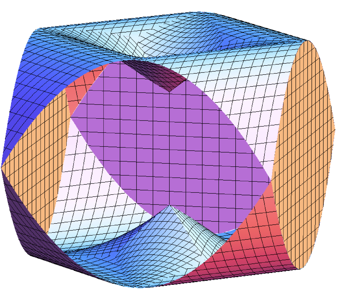
(a) Sphere

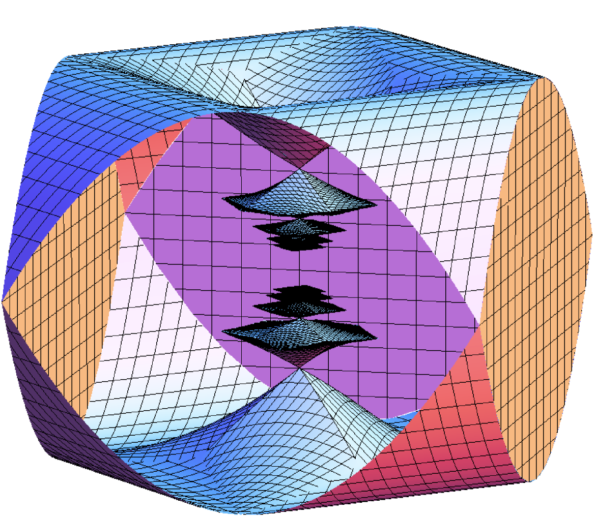
(b) Front

Figure 3. Sphere and front of the unit sphere in the Heisenberg group

5. Grushin structures

In this section we provide a description of the time-minimizing trajectories in two different sub-$\ell^{\infty}$ structures in the Grushin plane.

The classical sub-Riemannian structure on the Grushin plane is the metric structure on $\mathbb{R}^{2}$ determined by the choice of the orthonormal vector fields

$$X_{1}=\partial_{x},\qquad X_{2}=x\partial_{y}.$$

In other words the sub-Riemannian distance is characterized as follows

$$d(p_{1},p_{2})=\inf\left\{\int_{0}^{T}\sqrt{u_{1}^{2}+u_{2}^{2}}dt\,\bigg{|}\,\dot{\gamma}=u_{1}X_{1}(\gamma)+u_{2}(t)X_{2}(\gamma),\,\gamma(0)=p_{0},\,\gamma(1)=p_{1}\right\}.$$

The geodesic problem for this distance is equivalent to the time-optimal control problem defined by $X_{1}$, $X_{2}$ and $u(t)\in B$, where $B=\{u_{1}^{2}+u_{2}^{2}\leq 1\}$ is the standard Euclidean ball.

Due to the lack of symmetry of the Grushin structure, it is meaningful to consider two different sub-$\ell^{\infty}$ structures on the Grushin plane.

5.1. The first structure

Consider the sub-$\ell^{\infty}$ structures on $\mathbb{R}^{2}$ determined by the vector fields

(19) $$Y_{1}=\partial_{x}+x\partial_{y},\qquad Y_{2}=\partial_{x}-x\partial_{y}.$$

Notice that $Y_{1}=X_{1}+X_{2}$ and $Y_{2}=X_{1}-X_{2}$, so that we are considering the sub-$\ell^{1}$ sub-Finsler structure associated with $X_{1}$, $X_{2}$, up to a dilation factor. Similarly as in the Heisenberg group, let us introduce the vector field $Y_{3}=\partial_{y}$.

The Lie algebra generated by $Y_{1},Y_{2},Y_{3}$ actually satisfies the same commutator relations as in the Heisenberg group, namely

(20) $$[Y_{1},Y_{2}]=Y_{3},\qquad[Y_{1},Y_{3}]=[Y_{2},Y_{3}]=0.$$

The identities (20) gives the same equations (17) obtained in the Heisenberg case for the switching functions along an extremal trajectory

(21) $$\dot{\varphi}_{1}=-u_{2}\varphi_{3},\qquad\dot{\varphi}_{2}=u_{1}\varphi_{3},\qquad\dot{\varphi}_{3}=0.$$

In particular, $\varphi_{3}$ is constant. From the relation $Y_{2}-Y_{1}=xY_{3}$ we have the additional relation

(22) $$\varphi_{2}-\varphi_{1}=x\varphi_{3}.$$

In the case $\varphi_{3}=0$, we get $\varphi_{2}\equiv\varphi_{1}$ equals a constant, which is different from zero since the covector cannot be identically zero. Hence $u_{1},u_{2}$ are both $1$ or both $-1$. In other words, every trajectory corresponding to $\varphi_{3}=0$ is a horizontal line. Such curves are indeed time-minimizers.

Let us then consider the case $\varphi_{3}\neq 0$. Under this assumption, if both $\varphi_{1}$ and $\varphi_{2}$ are vanishing then the trajectory is abnormal. In particular relation (22) implies that $x(t)=0$ along the trajectory, hence we deduce that the trajectory is reduced to a point which is contained in the $y$-axis.

Lemma 11.

The only abnormal arcs on the sub-$\ell^{\infty}$ structure on $\mathbb{R}^{2}$ defined by the vector fields (19) are the constant curves contained in the set $\{x=0\}$. Consequently, no minimizer joining two distinct points is abnormal.

An analogous reasoning shows that there are no $\varphi_{1}$-singular (resp. $\varphi_{2}$-singular) trajectories that are not abnormal. Indeed assume the trajectory is $\varphi_{1}$-singular. Then $\varphi_{1}(t)=0$ for all $t$, that implies, by (21), that $u_{2}=0$ for all $t$ (recall that we are in the case $\varphi_{3}\neq 0$). Thus $\varphi_{2}$ is necessarily identically zero and the trajectory is actually abnormal. The situation is analogue for $\varphi_{2}$-singular trajectories.

Following the lines of Lemma 9 one can then show that, if the trajectory is not abnormal, then it is bang-bang, and all internal arcs of a bang-bang trajectory have the same length $s$.

Lemma 12.

On the sub-$\ell^{\infty}$ structure on $\mathbb{R}^{2}$ defined by the vector fields (19) the trajectories that have a regular arc are regular bang-bang. Moreover, all arcs have the same length $s$ except possibly the last and the first arc, whose lengths are less than or equal to $s$. At the junction between regular arcs the components $u_{1}$ and $u_{2}$ of the control switch sign alternately.

5.1.1. Bound on number of optimal regular arcs

Notice that if a bang-bang trajectory has an internal bang arc whose length is $t$, then $u_{1}$ and $u_{2}$ switch on the lines $x=\pm t/2$ (see Figura 4).

Regarding optimality, we claim that a bang-bang trajectory with $4$ bang arcs is not optimal. Indeed, every extremal trajectory starting from $y$-axis is not optimal after it intersects again the vertical axis, as it follows by replacing the trajectory by its reflection along the $y$-axis.

5.1.2. Optimal trajectories and shape of the unit ball

The picture of the regular bang bang trajectories for this structure on the Grushin plane is given in Figure 4. The corresponding picture of the unit ball is obtained in Figure 5.

Figure 4. Regular bang-bang trajectories for the Grushin structure (19)

Figure 5. The unit sphere and its front for the Grushin structure (19)

5.2. The second structure

We consider now the sub-$\ell^{\infty}$ structure on $\mathbb{R}^{2}$ determined by the vector fields

(23) $$X_{1}=\partial_{x},\qquad X_{2}=x\partial_{y}.$$

and we introduce the vector field $X_{3}=\partial_{y}$.

The Lie algebra generated by $X_{1},X_{2},X_{3}$ again satisfies the same commutator relations as in the Heisenberg group, namely

$$[X_{1},X_{2}]=X_{3},\qquad[X_{1},X_{3}]=[X_{2},X_{3}]=0.$$

Thus the identity (8) gives the analog equations (17) for the switching functions along an extremal trajectory

(24) $$\dot{\varphi}_{1}=-u_{2}\varphi_{3},\qquad\dot{\varphi}_{2}=u_{1}\varphi_{3},\qquad\dot{\varphi}_{3}=0,$$

In particular, $\varphi_{3}$ is constant. From $X_{2}=xX_{3}$ we have the additional relation

$$\varphi_{2}=x\varphi_{3}.$$

In the case $\varphi_{3}=0$, we get $\varphi_{2}\equiv 0$ and $\varphi_{1}$ equals a nonzero constant (otherwise the covector is identically zero). Reasoning as in Lemma 8, we have immediately the following result

Lemma 13.

On the sub-$\ell^{\infty}$ structure on $\mathbb{R}^{2}$ defined by the vector fields (23) the nonconstant trajectories that have singular arcs are exactly those for which $u_{1}$ is constantly equal to $1$ or $-1$. All of them consist of a single singular arc and are time-minimizers.

Let us then assume in what follows $\varphi_{3}\neq 0$.

Lemma 14.

The only abnormal arcs on the sub-$\ell^{\infty}$ structure on $\mathbb{R}^{2}$ defined by the vector fields (23) are the constant curves contained in the $y$-axis. Consequently, no minimizer joining two distinct points is abnormal.

If $\varphi_{3}\neq 0$ and the trajectory is not abnormal, then as in Lemma 9 it is regular bang-bang, all arcs have the same length $s$ except possibly the last and the first one, whose lengths are less than or equal to $s$. At the junction between bang arcs the components $u_{1}$ and $u_{2}$ of the control switch sign alternately.

Moreover, on a regular bang-bang trajectory, $u_{2}$ switches on the line $x=0$, since, if $\varphi_{2}(t)=0$ at a point $t$, then $x(t)\varphi_{3}=0$. Therefore if a bang-bang trajectory has an internal bang arc whose length is $s$, then $u_{1}$ switches on the lines $x=\pm s$. Moreover, at $u_{1}$-switching times the function $u_{1}$ goes from $1$ to $-1$ if the switch occurs in the half-plane $x>0$ while it goes from $-1$ to $1$ in the half-plane $x<0$, since

$${\rm sign}(\dot{\varphi}_{1})=-{\rm sign}(u_{2}\varphi_{3})=-{\rm sign}(\varphi_{2}\varphi_{3})=-{\rm sign}(x\varphi_{3}^{2})=-{\rm sign}(x).$$

5.2.1. Bound on number of optimal regular arcs

Regarding optimality, we prove the following lemma.

Lemma 15.

A regular bang-bang trajectory with more than $3$ arcs is not optimal. If, moreover, the trajectory starts on the $y$-axis and it is optimal, then it has at most $2$ arcs.

Proof.

First notice that, contrarily to what happens in the Heisenberg case, the role of the two vector fields $X_{1}$, $X_{2}$ is not symmetric. The replacement of $(u_{1},u_{2})$ by $(-u_{1},-u_{2})$ coupled with the reversion in the order of bangs, on the contrary, still yields a symmetric, equivalent, situation. This is a general fact, since it simply corresponds to reverse the parameterization of the curve. Looking at regular bang-bang trajectories (see Figure 7) one immediately recognizes that the proof of the lemma can be given by looking at two types of bang-bang trajectories, whose successive values of the control are

$$(1,-1),(1,1),(-1,1),(-1,-1)\quad\mbox{ and }\quad(1,1),(-1,1),(-1,-1),(1,-1),$$

respectively. In the first case, one notices that reflecting the second and third bang arcs with respect to the $y$-axis yields another horizontal curve with the same length, which is not extremal. Hence the curve is not optimal. This argument also shows that regular bang-bang trajectories starting from the $y$-axis and with more than 2 bang arcs are not optimal.

In the second case, let us apply Theorem 5 at the second switching time. One gets

$$Z_{0}=X_{1}+X_{2}+2sX_{3},\qquad Z_{1}=-X_{1}+X_{2},\qquad Z_{2}=-X_{1}-X_{2},\qquad Z_{3}=X_{1}-X_{2}+2sX_{3}.$$

Parameterizing the space $W$ by the coordinates $\alpha_{0},\alpha_{1}$ we get that $W=\{(\alpha_{0},\alpha_{1},-\alpha_{1},-\alpha_{0})\mid\alpha_{0},\alpha_{1}\in\mathbb{R}\}$. Normalizing $\varphi_{3}=1$ (uniqueness of the covector up to a positive factor is proved as in the case of the Heisenberg group), we write the quadratic form $Q$ as

$$Q(\alpha_{0},\alpha_{1})=2\alpha_{0}^{2}+4\alpha_{0}\alpha_{1}-2\alpha_{1}^{2}.$$

Since $Q(1,0)$ is positive, the considered trajectory is not optimal. This concludes the proof of Lemma 15. ∎

5.2.2. Optimal trajectories and shape of the unit ball

In this structure for the Grushin plane we have singular trajectories that are similar to the one obtained in the Heisenberg group, see Figure 6. Let us stress that in this case the tangent vector of the curve is forced to be inside a cone whose width increases with the $x$ coordinate.

Figure 6. Singular trajectories for the Grushin structure (23)

Regular bang bang trajectories from the origin are illustrated in Figure 7. These trajectories lose optimality as soon as they reach the vertical axes.

Figure 7. Bang-bang trajectories for the Grushin structure (23)

The picture of the unit ball in the Grushin plane with this structure is in Figure 8.

(a) Sphere

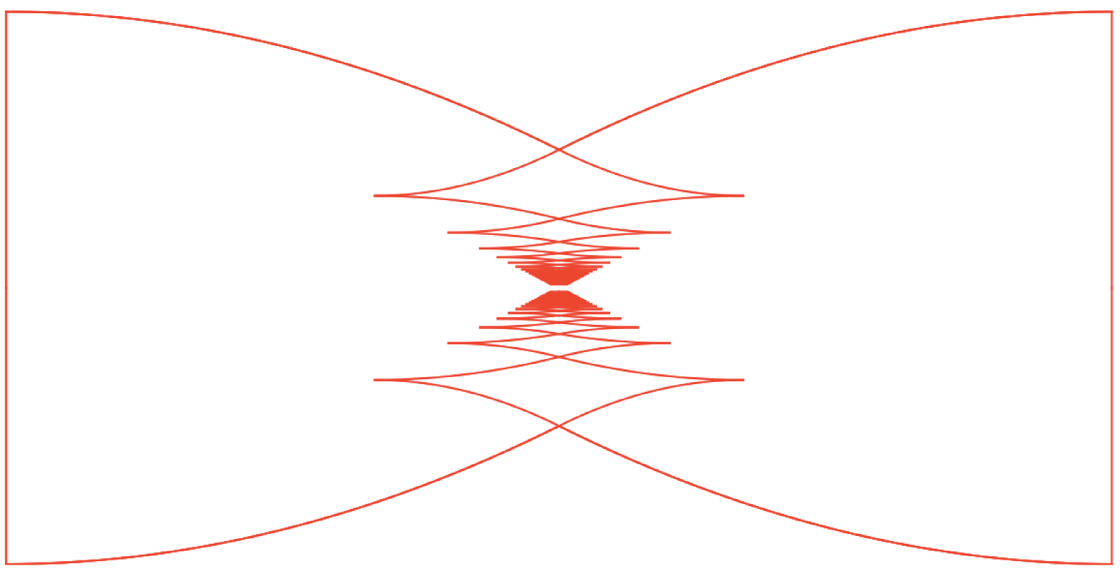
(b) Front

Figure 8. Sphere and front of the unit sphere for the Grushin structure (23)

6. Martinet structures

In this section we provide a description of the time-minimizing trajectories for two different sub-$\ell^{\infty}$ structures associated with the Martinet distribution. This is the easiest example where nontrivial abnormal minimizers appear.

The classical sub-Riemannian structure on the Martinet space is the metric structure on $\mathbb{R}^{3}$ determined by the choice of the orthonormal vector fields

$$X_{1}=\partial_{x}+y^{2}\partial_{z},\qquad X_{2}=\partial_{y}.$$

The sub-Riemannian distance is then

$$d(p_{1},p_{2})=\inf\left\{\int_{0}^{T}\sqrt{u_{1}^{2}+u_{2}^{2}}dt\,\bigg{|}\,\dot{\gamma}=u_{1}X_{1}(\gamma)+u_{2}(t)X_{2}(\gamma),\,\gamma(0)=p_{0},\,\gamma(1)=p_{1}\right\}.$$

The geodesic problem for this distance is equivalent to the time-optimal control problem defined by $X_{1},X_{2}$ and $u(t)\in B=\{u_{1}^{2}+u_{2}^{2}\leq 1\}$.

As in the case of the Grushin plane, due to the lack of symmetry, we are lead to consider two different sub-$\ell^{\infty}$ structures.

6.1. The first structure

Consider the sub-$\ell^{\infty}$ structure on $\mathbb{R}^{3}$ determined by the vector fields

(25) $$Y_{1}=\partial_{x}+\partial_{y}+y^{2}\partial_{z},\qquad Y_{2}=\partial_{x}-\partial_{y}+y^{2}\partial_{z}.$$

Notice that $Y_{1}=X_{1}+X_{2}$ and $Y_{2}=X_{1}-X_{2}$, so that we are considering the sub-$\ell^{1}$ Finsler structure defined by $X_{1}$ and $X_{2}$, up to a dilation factor. In analogy to the other cases, let us introduce the following vector fields defined by the commutators of the elements of the basis of the distribution

(26) $$Y_{3}:=[Y_{1},Y_{2}]=4y\partial_{z},\quad Y_{4}:=[Y_{1},[Y_{1},Y_{2}]]=4\partial_{z},\quad Y_{5}:=[Y_{2},[Y_{1},Y_{2}]]=-4\partial_{z}.$$

The switching functions associated with these vector fields and with an extremal pair $(\lambda(\cdot),\gamma(\cdot))$ are

$$\varphi_{i}(t)=\langle\lambda(t),Y_{i}(\gamma(t))\rangle,\qquad i=1,\ldots,5.$$

They satisfy the following system of differential equations

(27) $$\dot{\varphi}_{1}=-u_{2}\varphi_{3},\qquad\dot{\varphi}_{2}=u_{1}\varphi_{3},\qquad\dot{\varphi}_{3}=u_{1}\varphi_{4}+u_{2}\varphi_{5},$$

$$\dot{\varphi}_{4}=0,\qquad\dot{\varphi}_{5}=0.$$

Remark 16.

It follows from the bracket relations (26) that $\varphi_{4}$ and $\varphi_{5}=-\varphi_{4}$ are constants and we have $\varphi_{3}=y\varphi_{4}=-y\varphi_{5}$. In particular, if $\varphi_{4}=0$, then $\varphi_{3}$ is also constantly equal to zero, and $\varphi_{1},\varphi_{2}$ are constant.

Lemma 17.

The nontrivial abnormal arcs on the sub-$\ell^{\infty}$ structure on $\mathbb{R}^{3}$ defined by the vector fields (25) are the horizontal lines contained in the plane $\{y=0\}$.

Proof.

Assume that the trajectory is not reduced to a point and it is abnormal on some interval $I$. In particular we have $\varphi_{1}(t)=\varphi_{2}(t)=0$ for all $t\in I$, while its control $(u_{1}(t),u_{2}(t))$ is not identically zero on $I$. From identities (27) one immediately gets that $-u_{2}(t)\varphi_{3}(t)=u_{1}(t)\varphi_{3}(t)=0$. Hence, if we have that $\varphi_{3}(t)=y(t)\varphi_{4}=0$ for every $t$ (recall that $\varphi_{4}$ is constant), then $y(t)=0$ for all $t\in I$, otherwise $\varphi_{4}=0$ and the covector is identically zero. In particular $u_{1}=u_{2}$ on $I$ and the trajectory is contained in a line $\{y=0,z=z_{0}\}$. ∎

Remark 18.

Every costant trajectory (i.e., such that $u_{1}(t)=u_{2}(t)=0$ on $[0,T]$) is also abnormal.

The classification of extremal trajectories on Martinet is then reduced to regular and those that are singular with respect to exactly one control.

6.1.1. Singular arcs

Let us now consider a singular arc. We show that in this case we can recover its (singular) control by differentiation of the adjoint equations.

Indeed assume that the trajectory is $\varphi_{1}$-singular, i.e., $\varphi_{1}\equiv 0$ on $I$, and we want to recover its associated control $u_{1}$. Notice that $|u_{2}|=1$ is constant and $\dot{\varphi}_{1}=-u_{2}\varphi_{3}$. By singularity assumptions $\dot{\varphi}_{1}(t)\equiv 0$, that implies $\varphi_{3}(t)\equiv 0$ for all $t\in I$. We deduce that either $\varphi_{4}=0$ or $u_{1}=u_{2}$ on $I$. We have two possibilities::

• if $\varphi_{4}=0$ then $u_{1}$ is free,

• if $\varphi_{4}\neq 0$ then $u_{1}=u_{2}$ and the singular arc is also a bang arc, with no constraint on its length. Moreover $y=0$ on such an arc.

The situation with $\varphi_{2}$-singular arcs is perfectly symmetric.

6.1.2. Regular arcs

Assume that both $\varphi_{1}(0),\varphi_{2}(0)\neq 0$ (the same holds for small times by continuity). Because of Remark 16, we can assume that $\varphi_{4}\neq 0$ (otherwise the trajectory is made of a single bang arc). We want to show that

• When $\varphi_{1}(0)\varphi_{2}(0)>0$ then the two switching functions are affine in a right-neighborhood of $0$.

• When $\varphi_{1}(0)\varphi_{2}(0)<0$ the two switching functions are quadratic in a right-neighborhood of $0$.

On a bang arc the controls satisfy $|u_{1}|=|u_{2}|=1$ and thus we can differentiate the identity (27) and get

$$\ddot{\varphi}_{1}=-u_{2}\dot{\varphi}_{3}=-4u_{2}(u_{1}-u_{2})\varphi_{4},\quad\ddot{\varphi}_{2}=u_{1}\dot{\varphi}_{3}=4u_{1}(u_{1}-u_{2})\varphi_{4}.$$

In case (a) we have that $u_{1}=u_{2}=\pm 1$, which implies $\ddot{\varphi}_{1}=\ddot{\varphi}_{2}=0$. In case (b) we have $u_{1}-u_{2}=\pm 2$ and consequently $\ddot{\varphi}_{1}$ and $\ddot{\varphi}_{2}$ are constant and nonzero (recall that $\varphi_{4}\neq 0$ is constant). The equations for case (a) are

$$\varphi_{1}(t)=\varphi_{1}(0)+t\dot{\varphi}_{1}(0)=\varphi_{1}(0)-u_{2}\varphi_{3}(0)t,$$

$$\varphi_{2}(t)=\varphi_{2}(0)+t\dot{\varphi}_{2}(0)=\varphi_{2}(0)+u_{1}\varphi_{3}(0)t,$$

$$\varphi_{3}(t)=\varphi_{3}(0).$$

Notice that $\varphi_{3}(0)=y(0)\varphi_{4}$ is zero if we start on the abnormal set. The equations for case (b) are

$$\varphi_{1}(t)=\varphi_{1}(0)-u_{2}\varphi_{3}(0)t-u_{2}(u_{1}-u_{2})\varphi_{4}\frac{t^{2}}{2},$$

$$\varphi_{2}(t)=\varphi_{2}(0)+u_{1}\varphi_{3}(0)t+u_{1}(u_{1}-u_{2})\varphi_{4}\frac{t^{2}}{2},$$

$$\varphi_{3}(t)=\varphi_{3}(0)+(u_{1}-u_{2})\varphi_{4}t.$$

In particular, the constant $\varphi_{4}$ determines the convexity of the quadratic arc of the switching functions.

Lemma 19.

A regular bang arc can enter in a singular arc only if the switching function is quadratic and has vanishing derivative at the switching point.

Proof.

Assume, for instance, that at some time $t_{0}\in I$ we have $\varphi_{1}(t_{0})=1$ and $\varphi_{2}(t_{0})=0$. Then the control $u_{1}(t)=\text{sign}\varphi_{1}(t)$ is constantly equal to 1 in a neighborhood $U_{t_{0}}$ of $t_{0}$ and since $\varphi_{3}$ is continuous we deduce that $\dot{\varphi}_{2}=u_{1}\varphi_{3}$ is also continuous in $U_{t_{0}}$. Since on the singular arc $\dot{\varphi}_{2}=0$, we conclude. ∎

Next we discuss the possible behavior of the switching functions for regular arcs. Let us assume that $\varphi_{1}(0)>0$ and $\varphi_{2}(0)<0$. In particular $\varphi_{1}$ and $\varphi_{2}$ are quadratic on a right-neighborhood of $0$.

We are reduced to three possible cases for the the switching function $\varphi_{1}$:

• it never vanishes in the quadratic part (we say that $\varphi_{1}$ is of type NI, for not intersecting),

• it vanishes in the quadratic part and is tangent to the zero level (type T for tangent),

• it vanishes in the quadratic part and is transversal to the zero level (type I for intersecting).

In Figure 9 we picture the switching functions when $\varphi_{1}$ is of type NI, while Figures 10 and 11 correspond to type T and type I, respectively.

Figure 9. Switching functions for the Martinet structure (25) when $\varphi_{1}$ is of type NI.

Figure 10. Switching functions for the Martinet structure (25) when $\varphi_{1}$ is of type T. The relation between the length of the third and fourth bang arcs can be easily deduced from the expression of the switching functions.

Figure 11. Switching functions for the Martinet structure (25) when $\varphi_{1}$ is of type I.

Assuming that there are only regular bang arcs along the trajectory (as it is always the case when $\varphi_{1}$ is of type NI or I) we have the following result.

Proposition 20.

The switching functions of a trajectory that has only regular bang arcs are periodic.

The proof of Proposition 20 is a simple consequence of the formulas of the switching functions and Lemma 19. When $\varphi_{1}$ is of type T, the only freedom is in the length of singular arcs. The order in which the switching occur is as in Figures 9, 10 and 11, up to the symmetry which sends $(\varphi_{1},\varphi_{2},\varphi_{3},\varphi_{4})$ into $(-\varphi_{1},-\varphi_{2},\varphi_{3},-\varphi_{4})$ (which corresponds to a reflection $y\to-y$).

Remark 21.

It is easy to see from equations (27) and Remark 16 that if $\varphi_{1}$ is of type I then the $y$ coordinate of the corresponding trajectory has constant sign. When restricting our attention to trajectories starting on the plane $\{y=0\}$, we can then exclude that $\varphi_{1}$ is of type I.

6.1.3. Bound on the number of regular arcs for optimal trajectories

The goal of this section is to prove the following result.

Proposition 22.

A bang-bang trajectory with at least one regular arc and with more than $7$ arcs (either bang or singular) is not optimal. If, moreover, the trajectory starts on the plane $\{y=0\}$ and has more than $5$ arcs, then it is not optimal.

The proof works by applying several times Theorem 5. We should distinguish trajectories for which the switching functions are of one of the three types NI, T, and I.

In order to reduce the number of cases to be studied, we use the fact that time-reversion and reflection $y\to-y$ lead to trajectories with equivalent optimality properties.

Switching functions of type NI

We start by considering $\varphi_{1}$ of the type NI, as in Figure 9.

Lemma 23.

A regular bang-bang trajectory of type NI with more than $5$ arcs is not optimal. If, moreover, the trajectory starts on the plane $\{y=0\}$ and has more than $3$ arcs, then it is not optimal.

Proof.

We prove the first part of the lemma by showing that concatenations of the type

(28) $$(1,-1),(1,1),(-1,1),(1,1),(1,-1)$$

are not optimal. All concatenations of $6$ bang arcs, indeed, contain a concatenation of this type, up to symmetries (see Figure 12).

For concatenations of type (28), applying Theorem 5 at the second switching time, we get by computations as the one seen in the previous sections that the space $W$ and the quadratic form $Q$ in the statement of Theorem 5 can be written as

$$W=\{(\alpha_{0},\alpha_{1},0,-\alpha_{1},-\alpha_{0})\mid\alpha_{0},\alpha_{1}\in\mathbb{R}\},\quad Q(\alpha_{0},\alpha_{1})=8(t_{1}\alpha_{0}^{2}+t_{2}\alpha_{0}\alpha_{1}).$$

Since $Q$ is not negative semidefinite, the corresponding trajectory is not optimal.

In order to conclude the proof of Lemma 23, notice that, by metric considerations, if the trajectory starts from the plane $\{y=0\}$, then it stops to be optimal at the middle of the third bang arc, see Figure 12. ∎

Switching functions of type T

We prove here the following result concerning trajectories corresponding to switching functions of the type T as in Figure 10.

Lemma 24.

A trajectory of type T with more than $7$ arcs is not optimal. If, moreover, the trajectory starts on the plane $\{y=0\}$ and has more than $5$ arcs, then it is not optimal.

Proof.

We first consider the situation where $t^{k}_{\mathrm{sing}}>0$ for every $k$. We notice that every concatenations of $8$ arcs contains, up to symmetries, a concatenation of $6$ arcs of the type

(29) $$(1,-1),(1,1),(-1,1),(-1,-1),(-1,1),(1,1).$$

(See Figure 13). We are going to show that a concatenation as in (29) is not optimal.

For concatenations of type (29), applying Theorem 5 at the third switching time (at which $y=0$), we get that the space $W$ and the quadratic form $Q$ in the statement of Theorem 5 are written as

$$W=\{(\alpha_{0},\alpha_{1},\alpha_{2},-\alpha_{0},\alpha_{0}-\alpha_{2},-\alpha_{0}-\alpha_{1})\mid\alpha_{0},\alpha_{1},\alpha_{2}\in\mathbb{R}\},$$

$$Q(\alpha_{0},\alpha_{1},\alpha_{2})=2(t_{2}-2t^{2}_{\mathrm{sing}})\alpha_{0}^{2}+8t_{2}\alpha_{0}\alpha_{1}+8t^{2}_{\mathrm{sing}}\alpha_{0}\alpha_{2}-4t^{2}_{\mathrm{sing}}\alpha_{2}^{2}.$$

Notice that $Q$ is not negative semidefinite, since $Q(\varepsilon,1/\varepsilon,0)=2\varepsilon^{2}(t_{2}-2t^{2}_{\mathrm{sing}})+8t_{2}>0$ for $\varepsilon$ small enough. Hence, the corresponding trajectory is not optimal.

In the case where $t^{2}_{\mathrm{sing}}=0$, a concatenation as in (29) reduces to a concatenation of $4$ bang arcs

$$(1,-1),(1,1),(-1,1),(1,1).$$

Considering the following arc, we recover a concatenation as in (28), for which the same computations as in the previous section show non-optimality.

The proof of Lemma 24 can be concluded as before by metric considerations for trajectories starting from the plane $\{y=0\}$, see Figure 13. ∎

Switching functions of type I

We consider here trajectories corresponding to switching functions of type I as in Figure 11. Notice that such trajectories never cross the plane $\{y=0\}$.

We prove the following result.

Lemma 25.

A regular bang-bang trajectory of type I with more than $5$ arcs is not optimal.

Proof.

By the same symmetry considerations as in the cases NI and T, we are left to prove that concatenations of the type

(30) $$(1,-1),(-1,-1),(-1,1),(1,1),(1,-1),(-1,-1)$$

and

(31) $$(-1,1),(1,1),(1,-1),(-1,-1),(-1,1),(1,1)$$

are not optimal (see Figure 14). Notice than in both cases the trajectory is contained in $\{y<0\}$.

The application of Theorem 5 to the two cases is very similar leading (computing the quadratic form $Q$ at the second switching time $\tau_{2}$) to the expressions

$$Q(\alpha_{0},\alpha_{1},\alpha_{2})=-4(t_{1}-t_{3})\alpha_{0}^{2}-4y(\tau_{2})\alpha_{0}\alpha_{1}-4(-2t_{2}+2t_{3}+y(\tau_{2}))\alpha_{0}\alpha_{2}-4(2t_{2}-t_{3}-y(\tau_{2}))\alpha_{2}^{2}$$

and

$$Q(\alpha_{0},\alpha_{1},\alpha_{2})=-4(t_{1}-t_{3})\alpha_{0}^{2}-4y(\tau_{2})\alpha_{0}\alpha_{1}-4(-2t_{1}+2t_{2}+y(\tau_{2}))\alpha_{0}\alpha_{2}-4(t_{1}-2t_{2}-y(\tau_{2}))\alpha_{2}^{2}$$

respectively. In both cases, since $y(\tau_{2})<0$, one has that $Q(\varepsilon,1/\varepsilon,0)=-4y(\tau_{2})+O(\varepsilon^{2})$ is positive for $\varepsilon$ small enough. Theorem 5 then allows to conclude that the corresponding trajectories are not optimal. ∎

6.1.4. Optimal trajectories and shape of the unit ball

Here we present the different pictures for the $(x,y)$-components of trajectories corresponding to switching functions of the form NI, T and I. The dashed lines correspond to the part of the trajectory which is no more optimal.

In the case of trajectories of type NI we have the behavior in Figure 12.

Figure 12. Regular bang-bang trajectories of type NI for the Martinet structure (25).

Trajectories of type T have singular arcs of arbitrary length (see two examples in Figure 13). Notice that the switching to singular always happens at points where $y=0$, namely on the Martinet surface.

Figure 13. Regular/singular bang trajectories of type T for the Martinet structure (25).

The last case is given by trajectories of type I (see Figure 14). In this case the trajectory is contained in a strip $y_{0}\leq y(t)\leq y_{1}$ with eiter $0<y_{0}$ or $y_{1}>0$.

Figure 14. Regular bang-bang trajectories of type I for the Martinet structure (25).

In view of the optimality results one gets the following picture of the unit ball in the Martinet structure (25), see Figures 15 and 16.

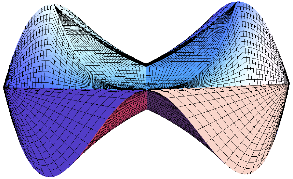
Figure 15. Unit sphere for the Martinet structure (25), view from the $x$-axis.

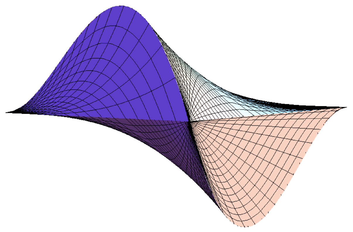
Figure 16. Unit sphere for the Martinet structure (25), view from the $y$-axis.

6.2. The second structure

The second sub-Finsler Martinet structure on $\mathbb{R}^{3}$ that we are going to consider is the sub-$\ell^{\infty}$ structure determined by the vector fields

(32) $$X_{1}=\partial_{x}+y^{2}\partial_{z},\qquad X_{2}=\partial_{y}.$$

We introduce the vector fields

(33) $$X_{3}:=[X_{1},X_{2}]=2y\partial_{z},\quad X_{4}:=[X_{1},[X_{1},X_{2}]]=0,\quad X_{5}:=[X_{2},[X_{1},X_{2}]]=2\partial_{z},$$

and the switching functions

$$\varphi_{i}(t)=\langle\lambda(t),X_{i}(\gamma(t))\rangle,\qquad i=1,\ldots,5.$$

The functions $\varphi_{i}$ satisfy the following system of differential equations

(34) $$\dot{\varphi}_{1}=-u_{2}\varphi_{3},\qquad\dot{\varphi}_{2}=u_{1}\varphi_{3},\qquad\dot{\varphi}_{3}=u_{1}\varphi_{4}+u_{2}\varphi_{5},\qquad\dot{\varphi}_{4}=0,\qquad\dot{\varphi}_{5}=0.$$

In this case the additional relations given by the bracket relations (33) are $\varphi_{3}=y\varphi_{5}$ and $\varphi_{4}=0$. In particular system (34) reduces to

(35) $$\dot{\varphi}_{1}=-u_{2}\varphi_{3},\qquad\dot{\varphi}_{2}=u_{1}\varphi_{3},\qquad\dot{\varphi}_{3}=u_{2}\varphi_{5},\qquad\dot{\varphi}_{5}=0.$$

Reasoning as in Lemma 17, we have the following characterization of abnormal arcs.

Lemma 26.

The nontrivial abnormal arcs on the sub-$\ell^{\infty}$ structure on $\mathbb{R}^{3}$ defined by the vector fields (32) are the horizontal lines contained in the plane $\{y=0\}$.

Indeed abnormal trajectories are described by the equations $\{y=0,z=z_{0}\}$. The fact that these trajectories are the same in the two Martinet structure under consideration reflects the fact that abnormal trajectories are independent of the choice of the frame (they depend only on the distribution).

6.2.1. Singular arcs

The situation is not in this case symmetric with respect to $\varphi_{1}$ and $\varphi_{2}$ singular. Let us first consider a $\varphi_{1}$-singular arc, i.e., $\varphi_{1}\equiv 0$ on $I$. Since $u_{2}=\pm 1$ is constant and $0\equiv\dot{\varphi}_{1}=-u_{2}\varphi_{3}$, it follows that $\varphi_{3}(t)=0$ for all $t\in I$. From $\dot{\varphi}_{3}=u_{2}\varphi_{5}$ we deduce that $\varphi_{5}=0$ and $u_{1}$ is arbitrary. In particular $\varphi_{3}$ is identically equal to zero, which implies that the trajectory stays singular for all times.

Let us then consider a $\varphi_{2}$-singular arc, i.e., $\varphi_{2}\equiv 0$ on $I$. Since $u_{1}=\pm 1$ is constant and $0\equiv\dot{\varphi}_{2}=u_{1}\varphi_{3}$ it follows that $\varphi_{3}(t)=0$ for all $t\in I$. We deduce that $0=\dot{\varphi}_{3}=u_{2}\varphi_{5}$. Hence, either $\varphi_{5}=0$ with $u_{2}$ arbitrary, or $u_{2}=0$ on $I$ with $\varphi_{5}\neq 0$. In the first case the trajectory stays singular for all times, in the second case the singular arc is contained in the plane $\{y=0\}$ and coincides with an abnormal trajectory on the interval $I$.

6.2.2. Regular arcs

The analysis is similar to that of the previous section. We therefore omit the computations, which yield the following result.

Proposition 27.

A regular trajectory with more than 6 arcs (either bang or singular) is not optimal.

The picture of the unit ball in the Martinet structure (32) is given in Figure 17.

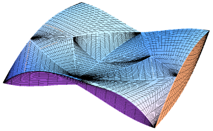
Figure 17. Unit sphere for the Martinet structure (32).

7. Euclidean rectifiability and semi-analyticity of spheres

By construction the $\ell^{\infty}$ spheres for the Heisenberg, Grushin and Martinet structures studied above are homeomorphic to Euclidean spheres ($S^{2}$ for Heisenberg and Martinet and $S^{1}$ for Grushin). Moreover these spheres are graphs of piecewise-polynomial functions.

It follows that these spheres are Euclidean rectifiable and semi-analytic. Theorem 2 follows.

References

- [ABCK97] A. Agrachev, B. Bonnard, M. Chyba, and I. Kupka, Sub-Riemannian sphere in Martinet flat case, ESAIM Control Optim. Calc. Var. 2 (1997), 377–448 (electronic).
- [AG90] A. A. Agrachëv and R. V. Gamkrelidze, Symplectic geometry for optimal control, Nonlinear controllability and optimal control, Monogr. Textbooks Pure Appl. Math., vol. 133, Dekker, New York, 1990, pp. 263–277.
- [AS03] Andrei A. Agrachev and Mario Sigalotti, On the local structure of optimal trajectories in , SIAM J. Control Optim. 42 (2003), no. 2, 513–531. MR 1982281 (2004f:49042)
- [AS04] Andrei A. Agrachev and Yuri L. Sachkov, Control theory from the geometric viewpoint, Encyclopaedia of Mathematical Sciences, vol. 87, Springer-Verlag, Berlin, 2004, Control Theory and Optimization, II.
- [BCC05] Ugo Boscain, Thomas Chambrion, and Grégoire Charlot, Nonisotropic 3-level quantum systems: complete solutions for minimum time and minimum energy, Discrete Contin. Dyn. Syst. Ser. B 5 (2005), no. 4, 957–990 (electronic).
- [Ber89a] Valeriĭ N. Berestovskiĭ, Homogeneous manifolds with an intrinsic metric. II, Sibirsk. Mat. Zh. 30 (1989), no. 2, 14–28, 225.
- [Ber89b] by same author, The structure of locally compact homogeneous spaces with an intrinsic metric, Sibirsk. Mat. Zh. 30 (1989), no. 1, 23–34.
- [BLD13] Emmanuel Breuillard and Enrico Le Donne, On the rate of convergence to the asymptotic cone for nilpotent groups and subFinsler geometry, Proc. Natl. Acad. Sci. USA 110 (2013), no. 48, 19220–19226.
- [BM46] Salomon Bochner and Deane Montgomery, Locally compact groups of differentiable transformations, Ann. of Math. (2) 47 (1946), 639–653.
- [CM06] Jeanne N. Clelland and Christopher G. Moseley, Sub-Finsler geometry in dimension three, Differential Geom. Appl. 24 (2006), no. 6, 628–651.
- [CM13] Michael G. Cowling and Alessio Martini, Sub-Finsler geometry and finite propagation speed, Trends in harmonic analysis, Springer INdAM Ser., vol. 3, Springer, Milan, 2013, pp. 147–205. MR 3026352
- [CMW07] Jeanne N. Clelland, Christopher G. Moseley, and George R. Wilkens, Geometry of sub-Finsler Engel manifolds, Asian J. Math. 11 (2007), no. 4, 699–726.
- [Gle52] Andrew M. Gleason, Groups without small subgroups, Ann. of Math. (2) 56 (1952), 193–212.
- [Gro99] Mikhail Gromov, Metric structures for Riemannian and non-Riemannian spaces, Progress in Mathematics, vol. 152, Birkhäuser Boston Inc., Boston, MA, 1999, Based on the 1981 French original, With appendices by M. Katz, P. Pansu and S. Semmes, Translated from the French by Sean Michael Bates.
- [LDNG15] Enrico Le Donne and Sebastiano Nicolussi Golo, Regularity properties of spheres in graded groups, In preparation (2015).
- [MT12] Vladimir S. Matveev and Marc Troyanov, The Binet-Legendre metric in Finsler geometry, Geom. Topol. 16 (2012), no. 4, 2135–2170.
- [MZ74] Deane Montgomery and Leo Zippin, Topological transformation groups, Robert E. Krieger Publishing Co., Huntington, N.Y., 1974, Reprint of the 1955 original.
- [Pan89] Pierre Pansu, Métriques de Carnot-Carathéodory et quasiisométries des espaces symétriques de rang un, Ann. of Math. (2) 129 (1989), no. 1, 1–60.
- [Sig05] M. Sigalotti, Local regularity of optimal trajectories for control problems with general boundary conditions, J. Dyn. Control Syst. 11 (2005), no. 1, 91–123. MR 2122468 (2005i:49002)