Demon Dynamics:
Deterministic Chaos, the Szilard Map, and
the Intelligence of Thermodynamic Systems

Abstract

We introduce a deterministic chaotic system—the Szilard Map—that encapsulates the measurement, control, and erasure protocol by which Maxwellian Demons extract work from a heat reservoir. Implementing the Demon’s control function in a dynamical embodiment, our construction symmetrizes Demon and thermodynamic system, allowing one to explore their functionality and recover the fundamental trade-off between the thermodynamic costs of dissipation due to measurement and due to erasure. The map’s degree of chaos—captured by the Kolmogorov-Sinai entropy—is the rate of energy extraction from the heat bath. Moreover, an engine’s statistical complexity quantifies the minimum necessary system memory for it to function. In this way, dynamical instability in the control protocol plays an essential and constructive role in intelligent thermodynamic systems.

Keywords: deterministic chaos, Lyapunov characteristic exponents, Markov partition, Landauer’s Principle, measurement, erasure, memory, entropy rate, mutual information, dissipated work, control theory

Synthetic nanoscale machines [1, 2, 3, 4], like their macromolecular biological counterparts [5, 6, 7], perform tasks that involve the simultaneous manipulation of energy, information, and matter. In this they are information engines—systems with two inextricably intertwined characters. The first aspect, call it “physical”, is the one in which the system—seen embedded in a material substrate—is driven by, manipulates, stores, and dissipates energy. The second aspect, call it “informational”, is the one in which the system—seen in terms of its spatial and temporal organization—generates, stores, loses, and transforms information. Information engines operate by synergistically balancing both aspects to support a given functionality, such as extracting work from a heat reservoir.

This is remarkable behavior. Though we can sometimes identify it—in a motor protein hauling nutrients across a cell’s microtubule highways [5], in how a quantum dot transistor modulates current under the influence of an evanescent wave function [8, 9]—it is not well understood. Understanding calls on a thermodynamics of nanoscale systems that operate far out of equilibrium and on a physics of information that quantitatively identifies organization and function, neither of which has been fully articulated. However, recent theoretical and experimental breakthroughs [6, 10, 11, 12, 7] hint that we may be close to a synthesis which not only provides understanding but predicts quantitative, measurable functionalities.

We define an information engine as a system that performs information processing as it undergoes controlled thermodynamic transformations. We show that information engines are chaotic dynamical systems. Building this bridge to dynamical systems theory allows us to employ its powerful tools to analyze an engine’s complex, nonlinear behavior. This includes a thorough informational and structural analysis that leads to a measure of thermodynamic system intelligence.

By way of concretely illustrating the theory, we introduce an explicit implementation of Szilard’s Engine [13] as an iterated composite map of the unit square that is a deterministic, but chaotic dynamical system. The result is a particularly simple and constructive view of the energetics and computation embedded in controlled nonlinear thermodynamical systems. That simplicity, however, gives a solid base for designing and analyzing real information engines. We end giving a concise statement of the general theory and applications.

Background

The Szilard Engine is an ideal Maxwellian Demon for examining the role of information processing in the Second Law [13]. The engine consists of three components: a controller (the Demon), a thermodynamic system (a particle in a box), and a heat bath that keeps both thermalized to a temperature $T$. It operates by a simple mechanism of a repeating three-step cycle of measurement, control, and erasure. During measurement, a barrier is inserted midway in the box, constraining the particle either to box’s left or right half, and the Demon memory changes to reflect on which side the particle is. In the thermodynamic control step, the Demon uses that knowledge to allow the particle to push the barrier, extracting $\int P~{}dV=k_{B}T\ln 2$ work from the thermal bath. (Supplementary Materials review this and related thermodynamic calculations.) In the erasure step, the Demon resets its finite memory to a default state, so that it can perform measurement again. The periodic protocol cycle of measurement, control, and erasure repeats endlessly and deterministically. The net result being the extraction of work from the bath balanced by entropy created by changes in the Demon’s memory.

Rather than seeing the Demon and box as separate, though, we view it—an information engine—as the direct product of thermodynamic system and Demon memory . Though we follow Szilard closely, he did not specify the Demon’s physical embodiment. Critically, we choose the Demon’s memory to be another spatial dimension of a particle in a box. Thus, we see the joint system as a single particle in a two-dimensional box, where one axis represents the thermodynamic System Under Study (SUS)—the original particle in a box—and the other axis represents the Demon memory. We now describe a deterministic protocol that implements the Szilard Engine, evolving a particle ensemble over the joint state space.

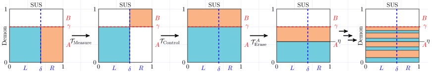
Figure 1: Szilard Engine as a deterministic dynamical system: the Szilard Map $\mathcal{T}_{\mathrm{Szilard}}=\mathcal{T}_{\mathrm{Erase}}^{A}\circ\mathcal{T}_{\mathrm{Control}}\circ\mathcal{T}_{\mathrm{Measure}}$. Regions left and right of $\delta$ colored to aid tracking particle location. Rightmost: action of $\mathcal{T}_{\mathrm{Szilard}}^{3}$ resulting in self-similar (fractal) structure in density $\widehat{\rho}$; uniform $\widehat{\rho}$ requires $\eta=\gamma\delta$. These assume the Demon’s reset memory state is $A$. (Supplementary Materials include an animation.)

A Dynamical Engine

The Szilard Engine’s measurement-control-erasure barrier-sliding protocol is equivalent to a discrete-time two-dimensional map from unit square $\mathbb{I}^{2}=[0,1]\times[0,1]$ to itself. The engine has two kinds of mesoscopic states—states of the particle’s location $\big{\{}L\sim x\in(0,\delta],R\sim x\in(\delta,1)\big{\}}$ and states of the Demon’s knowledge $\big{\{}A\sim y\in(0,\gamma],B\sim y\in(\gamma,1)\big{\}}$ of the location—that partition the joint states $(x,y)\in\mathbb{I}^{2}$.

The protocol cycle translates into a composite map $\mathcal{T}_{\mathrm{Szilard}}=\mathcal{T}_{\mathrm{E}}\circ\mathcal{T}_{\mathrm{C}}\circ\mathcal{T}_{\mathrm{M}}$ of $\mathbb{I}^{2}$; one map for each engine step; see Fig. 1(a). As they operate, they take the joint state space from one stage to another around the cycle:

Measurement:

To correlate Demon memory with particle location $\mathcal{T}_{\mathrm{M}}$ takes the $A\otimes L$ and the $B\otimes L$ mesostates to themselves, the $A\otimes R$ mesostate to $B\otimes R$, and $B\otimes R$ to $A\otimes R$:

$$\mathcal{T}_{\mathrm{M}}(x,y)=\begin{cases}(x,y)&x<\delta,y<\gamma\text{ or }x<\delta,y\geq\gamma~{},\\ \left(x,\gamma+y\frac{1-\gamma}{\gamma}\right)&x\geq\delta,y\leq\gamma~{},\\ \left(x,\gamma\frac{y-\gamma}{1-\gamma}\right)&x\geq\delta,y>\gamma~{}.\end{cases}$$

Thermodynamic control:

To extract energy from the bath $\mathcal{T}_{\mathrm{C}}$ expands both the $A$ and $B$ Demon memory mesostates over the SUS’s whole interval:

$$\mathcal{T}_{\mathrm{C}}(x,y)=\begin{cases}(\frac{x}{\delta},y)&x<\delta~{},\\ \left(\frac{x-\delta}{1-\delta},y\right)&x\geq\delta~{}.\end{cases}$$

Erasure:

$\mathcal{T}_{\mathrm{E}}$ maps both the $A$ and $B$ Demon memory mesostates back to a selected Demon memory reset mesostate. If that reset state is $A$, then the mapping is:

$$\mathcal{T}_{\mathrm{E}}^{A}(x,y)=\begin{cases}(x,y\delta)&y<\gamma~{},\\ \left(x,\delta\gamma+\frac{y-\gamma}{1-\gamma}\gamma(1-\delta)\right)&y\geq\gamma~{}.\end{cases}$$

This explicit construction establishes that Szilard’s Engine is a deterministic dynamical system whose component maps are thermodynamic transformations—a piecewise thermodynamical system. The mapping $\mathcal{T}_{\mathrm{Szilard}}$ means we can avail ourselves of the analytical tools of dynamical systems theory [15, 16] to analyze the Szilard Engine mechanisms. This perforce suggests a number of more refined and quantitative questions about the dynamics ranging from the structural role of the stable and unstable submanifolds in supporting information and thermodynamic processing and the existence of asymptotic invariant measures to measures of information generation, storage, and intelligence.

As typically done to establish a known initial state for any engineered computing device, we initialize the system first using $\mathcal{T}_{\mathrm{E}}$. The result is that $\mathcal{T}_{\mathrm{Szilard}}$ becomes the well known asymmetric Baker’s Map $\mathcal{T}_{\mathrm{Baker}}^{A}(x,y)=\mathcal{T}_{\mathrm{C}}\circ\mathcal{T}_{\mathrm{M}}\circ\mathcal{T}_{\mathrm{E}}^{A}$:

$$\mathcal{T}_{\mathrm{Baker}}^{A}(x,y)= \begin{cases}(\frac{x}{\delta},\delta y)&x<\delta~{},\\ \left(\frac{x-\delta}{1-\delta},\delta+y(1-\delta)\right)&x\geq\delta~{}.\end{cases}$$

The familiar stretching and folding action of $\mathcal{T}_{\mathrm{Baker}}$ is shown in Fig. S1(b) of the Supplementary Materials. Being a Baker’s map, it is immediately clear that the Szilard Engine dynamics are chaotic [15, 16].

While the overall composite map $\mathcal{T}_{\mathrm{Szilard}}$ is important, considering its complete-cycle behavior alone misses much. What is key are the component maps that nominally control a thermodynamic system, with each step corresponding to a different thermodynamic transformation. We now analyze the dynamics to see how the component maps contribute to information processing and thermodynamics. (Supplementary Materials give calculational details.)

Dynamical Systems Analysis

What does chaos in the Szilard Engine mean? The joint system generates information—the information about particle position that the Demon must keep repeatedly measuring to stay synchronized to the SUS and so extract energy from the bath. On the one hand, it is generated by the heat bath through state-space expansion during $\mathcal{T}_{\mathrm{C}}$. And, on the other, it is stored by the Demon (temporarily) and must be erased during $\mathcal{T}_{\mathrm{E}}$. The latter’s construction makes clear that it, dynamically, contracts state-space and so is locally dissipative.

With explicit equations of motion in hand, one can directly check, by calculating the Jacobian $\partial_{xy}\mathcal{T}_{\mathrm{Baker}}$, that the map is globally area preserving. Moreover, the invariant distribution $\widehat{\rho}$ can be determined from the Frobenious-Perron operator [15, 16]:

$$\widehat{\rho}(x^{\prime},y^{\prime})=\int_{\mathbb{I}^{2}}dxdy~{}\delta\big{(}(x^{\prime},y^{\prime})-\mathcal{T}_{\mathrm{Baker}}(x,y)\big{)}\widehat{\rho}(x,y)~{}.$$

($\delta(\cdot)$ here, and only here, is the Dirac delta-function.) Calculation shows that $\widehat{\rho}$ has full support on the unit square $\mathbb{I}^{2}$ and so its fractal dimension is $d_{f}=2$ for all $\delta,\gamma\in(0,1)$. The particle density is uniform when, during $\mathcal{T}_{\mathrm{E}}$, the Demon’s memory mesostate partition falls at $\eta=\gamma\delta$. However, when $\eta\neq\gamma\delta$, the density is not uniform, which is reflected in $\widehat{\rho}$’s information dimension $d_{I}<d_{f}$, [16, Chs. 11-12]. This corresponds to changing the efficiency of the Demon’s information extraction, which we see is reflected in the difference $d_{f}-d_{I}$.

The Szilard Map Jacobian also determines its local linearization and so one can easily calculate the spectrum of Lyapunov characteristic exponents (LCEs) for the overall cycle and so realize the contribution of each protocol step. This gives insight into the directions (submanifolds) of stability (convergence) and instability (divergence). There are two LCEs: one positive $\lambda^{+}=\operatorname{H}(\delta)$ and one negative $\lambda^{-}=-\operatorname{H}(\delta)$, where $\operatorname{H}(\delta)$ is the (base $2$) binary entropy function [17]. (See Supplementary Material for details.) Note that energy conservation ($\mathcal{T}_{\mathrm{Szilard}}$’s area preservation) is reflected in the exact balance of instability and stability: $\lambda^{+}+\lambda^{-}=0$. The unstable manifolds (parallel the $x$-axis) support the mechanism that amplifies small fluctuations from the heat bath to macroscopic scale during energy extraction ($\mathcal{T}_{\mathrm{C}}$). The stable manifolds (parallel the $y$-axis) are the mechanism that dissipates energy into the ambient heat bath, during erasure ($\mathcal{T}_{\mathrm{E}}$).

The overall information production rate is given by $\mathcal{T}_{\mathrm{Szilard}}$’s Kolmogorov-Sinai entropy $h_{\mu}$ [18]. For the Szilard Engine, given the well behaved nature of $\widehat{\rho}$, $h_{\mu}=\sum_{\lambda>0}\lambda=\lambda^{+}$ by Pesin’s Theorem [16]. (That is, $h_{\mu}=\operatorname{H}(\delta)$, directly verified shortly.) This measures the flow of information from the SUS into the Demon: information harvested from the bath and used by the Demon to convert thermal energy into work. Simply stated, the degree of chaos determines the rate of energy extraction from the bath.

Computational Mechanics Analysis

The Demon memory and particle location mesostates form Markov partitions for the Szilard Map dynamics [16, Chs. 7,9]: tracking sequences of symbols in $\{A,B\}$ or in $\{R,L\}$ (or all four pairs $\{AR,AL,BR,BL\}$) leads to a symbolic dynamics that captures all of the joint system’s information processing behavior. We now use this fact to analyze the various kinds of information processing and introduce a way to measure the Demon’s “intelligence” or, more appropriately, that of the entire engine. We do this by calculating computational mechanics’ $\epsilon$-machines and $\epsilon$-transducers from the engine’s symbolic dynamics [19, 20]. The overall engine transducer is shown in Fig. 2(a), that for the SUS particle dynamics in Fig. S2(a), and for the Demon memory dynamics in Fig. S2(b).

In addition to explicitly expressing the effective mechanisms that support information processing, $\epsilon$-machines allow us to quantify the effects of measurement, control, and erasure. The engine’s Kolmogorov-Sinai entropy $h_{\mu}$ can be calculated directly from the $\epsilon$-machines’s causal-state averaged transition uncertainty. To quantitatively measure the minimal required memory—a key component of “intelligence”—for the information engine functioning, we employ the $\epsilon$-machine’s statistical complexity $C_{\mu}=\operatorname{H}[\Pr(\sigma)]$, where $\sigma\in\bm{\mathcal{S}}$ are the system’s causal states [19] and $\operatorname{H}[\cdot]$ is the Shannon information [17].

(a)                              (b)

Figure 2: $\epsilon$-Transducers for the symbolic dynamics of the Szilard information engine from the Markov partition of its joint state space: (a) The $\epsilon$-transducer for $\mathcal{T}_{\mathrm{Szilard}}$ that reads in the periodic control signal for measure ($M$), control (C), and erase (E). (b) $\mathcal{T}_{\mathrm{Szilard}}$ single-state $\epsilon$-transducer: Memoryless over the full measure-control-erase protocol. Transitions $\beta|\alpha:p$ denote reading protocol symbol $\alpha$, taking the transition with probability $p$, emitting symbol $\beta$. Asymptotic state probabilities are given in parentheses underneath state names.

It is important to emphasize an aspect of the information engine $\epsilon$-machine construction: It is stage-dependent in that, to fully capture the component operations and their thermodynamic effects, the individual maps must to taken into account. This observation should be contrasted with the symbolic dynamics and particle position $\epsilon$-machine for the overall Szilard map in its Baker’s map form. The resulting process arises from stroboscopically observing the behavior after driving the engine with the three-symbol word $MCE$. As an example, the particle position process’s $\epsilon$-machine is shown in Fig. 2(b); it is a biased coin—a single-state $\epsilon$-machine with no memory: $C_{\mu}(\mathcal{T}_{\mathrm{Baker}})=0$. This is as it should be: The overall cycle must return to the same state storing no memory of previous cycles.

Computational mechanics analysis shows that, over the three-step cycle, the Engine has an entropy rate of $h_{\mu}=\operatorname{H}(\delta)$ as seen above (or $\operatorname{H}(\delta)/3$ per map step) and a statistical complexity of $C_{\mu}=\log_{2}3+\operatorname{H}(\delta)$. (See Supplementary Materials for details, including analysis of SUS and Demon subsystems.) How predictable is the Engine’s operation? The information in its future predictable from its past is given by the excess entropy: ${\bf E}=\operatorname{I}[\smash{\overleftarrow{Z}};\smash{\overrightarrow{Z}}]$, where $\smash{\overleftarrow{Z}}$ is the past and $\smash{\overrightarrow{Z}}$ is the future of the joint process over random variable $Z_{t}\in\{A,B\}\otimes\{R,L\}$. We see that the machine in Fig. 2(a), driven by the protocol, is counifilar and so ${\bf E}=C_{\mu}$ [21].

Thermodynamics

During each protocol step the Engine interacts thermodynamically with the heat bath. The Supplementary Materials calculate the average heat $\braket{Q}$ and work $\braket{W}$ flows between the Demon and the bath and between the SUS and the bath during each step. For the Szilard Engine heat and work are equivalent and so we discuss only the heat as energies $\braket{Q_{\text{diss}}}$ dissipated to the bath for each interaction. As we will see, although $\gamma$—the Demon memory partition—did not play a direct role in the informational properties, it does in the thermodynamics.

The expected heat flow during measurement is $\braket{Q_{\mathrm{measure}}}=-k_{B}T(1-\delta)\ln\left((1-\gamma)/\gamma\right)$. Since $\gamma\in[0,1]$, the dissipated heat can be negative or positive. It vanishes at $\gamma=1/2$. Negative dissipated heat means that the engine absorbs energy from the heat bath and, in that case, turns it into work. The work $\int P~{}dV$ done by the particle on the barrier is $k_{B}T\operatorname{H}(\delta)\ln 2$. Thus, the average heat absorbed by the engine from the heat bath during thermodynamic control is $\braket{Q_{\mathrm{control}}}=-k_{B}T\operatorname{H}(\delta)\ln 2$, which is maximized when $\delta=1/2$. During memory erasure the Demon shifts back to its default state, without affecting the SUS state. The barrier partitioning the Demon’s mesostates slides, compressing the contained particle into the default state $A$, say. The heat dissipated in this process is $\braket{Q_{\mathrm{erase}}}=k_{B}T(1-\delta)\ln\left((1-\gamma)/\gamma\right)+k_{B}T\operatorname{H}(\delta)\ln 2$.

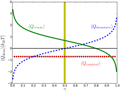
Figure 3: Beyond Landauer’s Principle: Thermodynamic costs (energy dissipation $Q_{\mathrm{diss}}$) for measurement, control, and erasure in Szilard’s information engine as a function of $\gamma$ (Demon partition) with SUS barrier at $\delta=1/2$. Landauer’s Principle applies only at $\gamma=1/2$ (vertical yellow band): measurements are thermodynamically free, erasure costs since heat is dissipated as a result of Demon resetting. Costs exactly flip at $\gamma=4/5$, though.

While the heat dissipated during control is independent of $\gamma$, both measurement and erasure can dissipate any positive or negative amount of heat, depending on $\gamma$. Notably, for $\gamma>1/2$, the Szilard Engine violates Landauer’s Principle [22, 23] in that $\braket{Q_{\mathrm{erase}}}\leq\ln 2$; in energy units of $k_{B}T$. Indeed, for $\gamma=4/5$, erasure is thermodynamically free and measurement is costly—an anti-Landauer Principle.

Figure 3 illustrates the trade-offs in thermodynamic costs for each step. They sum to zero and so the Engine respects the Second Law over the whole range of $\delta$ and $\gamma$. The erasure and measurement steps together obey the relation: $\braket{Q_{\mathrm{erase}}}+\braket{Q_{\mathrm{measure}}}=k_{B}T\operatorname{H}(\delta)\ln 2$, recovering trade-offs noted previously [24, 25, 26, 27]. That is, the Szilard Engine achieves the lower bounds on energy dissipation during measurement and erasure. And so, it plays an analogous optimal role in the conversion of information into work as the Carnot Engine does for optimal efficiency when converting thermal energy to work.

Final Remarks

We leveraged a straightforward observation to give a thorough dynamical systems, computational mechanics, and thermodynamic analysis of Szilard’s Engine: an information engine’s intrinsic computation is supported by the evolution of its joint state-space distribution and its thermodynamic costs monitor how those distributional changes couple energetically to its environment.

The Szilard Map construction is straightforward and easy to interpret. For these reasons, we selected it to illustrate the bridge between thermodynamics, information theory, and dynamical systems necessary to fully analyze information engines. The approach generalizes. We can now state our central proposal: (i) an information engine is the dynamic over a joint state space of a thermodynamic system and a physically embodied controller, (ii) the causal states of the joint dynamics, formed from the predictive equivalence classes of system histories, capture its information processing and emergent organization, (iii) a necessary component of the engine’s effective “intelligence”, its memory, is given by its statistical complexity $C_{\mu}$, (iv) its dissipation is given by the dynamical system negative LCEs, and (v) the rate of energy extracted from the heat bath is governed by the Kolmogorov-Sinai entropy $h_{\mu}$.

Sequels use this approach to analyze the information thermodynamics of more sophisticated engines, including the Mandal-Jarzynski ratchet [28], experimental nanoscale information processing devices, and intelligent macromolecules.

Supplementary Materials:

Calculational details, further discussion and interpretation, and animation illustrating a continuous-time embedding of $\mathcal{T}_{\mathrm{Szilard}}$.

Supplementary Materials

I Szilard Map Construction Details

Here, we mention several details underlying the construction of $\mathcal{T}_{\mathrm{Szilard}}$ and $\mathcal{T}_{\mathrm{Baker}}$. There is, in fact, a family of related maps. Partly, this comes from the incompleteness of Szilard’s presentation Futz_Szil29a; partly, due to possible, permitted variations in implementation. The following comments only hint at these variations. A sequel will develop them more systematically.

Erasure:

$\mathcal{T}_{\mathrm{E}}$ maps both the $A$ and $B$ Demon memory mesostates back to a selected Demon memory reset mesostate. If that reset state is $A$, then the mapping is:

$$\mathcal{T}_{\mathrm{E}}^{A}(x,y)=\begin{cases}(x,y\delta)&y<\gamma~{},\\ \left(x,\delta\gamma+\frac{y-\gamma}{1-\gamma}\gamma(1-\delta)\right)&y\geq\gamma~{}.\end{cases}$$

If the reset state is $B$, then the mapping is:

$$\mathcal{T}_{\mathrm{E}}^{B}(x,y)=\begin{cases}\left(x,\gamma-y+\frac{y}{\gamma}\left(1-\delta(1-\gamma)\right)\right)&y<\gamma~{},\\ \left(x,1-\delta(1-y)\right)&y\geq\gamma~{}.\end{cases}$$

The cell boundary required by area preservation (probability invariance) under map $\mathcal{T}_{\mathrm{E}}^{A}$ is $y^{\prime}=\delta\gamma$ and for map $\mathcal{T}_{\mathrm{E}}^{B}$, $y^{\prime}=1-\delta(1-\gamma)$. The reason for this is that during the control operation horizontal stretching by $\delta^{-1}$ or by $(1-\delta)^{-1}$ “dilutes the gas” or reduces the probability density. To maintain probability invariance (or “gas density”) we must compensate in the erase operation by multiplying the Demon (vertical) coordinate by $\delta$ or $1-\delta$.

Full cycle operation:

The overall information engine cycle, then, is the map given by the composition of the component maps: $\mathcal{T}_{\mathrm{Szilard}}=\mathcal{T}_{\mathrm{E}}^{A}\circ\mathcal{T}_{\mathrm{C}}\circ\mathcal{T}_{\mathrm{M}}$. The action of $\mathcal{T}_{\mathrm{Szilard}}$ is shown in Fig. S1(a), where $\eta=\gamma\delta$. The map is area preserving, as is verified below by calculating the determinant of its Jacobian.

Initial-reset engine:

If one first resets the engine with $\mathcal{T}_{\mathrm{E}}^{A}$, then we obtain the familiar Baker’s Map $\mathcal{T}_{\mathrm{Baker}}=\mathcal{T}_{\mathrm{C}}\circ\mathcal{T}_{\mathrm{M}}\circ\mathcal{T}_{\mathrm{E}}^{A}$:

$$\mathcal{T}_{\mathrm{Baker}}(x,y)= \begin{cases}(\frac{x}{\delta},\delta y)&x<\delta~{},\\ \left(\frac{x-\delta}{1-\delta},\delta+y(1-\delta)\right)&x\geq\delta~{}.\end{cases}$$

It’s action on the joint state space is show in Fig. S1(b).

Due to several choices in the construction of the component maps, the two distinct $\mathcal{T}_{\mathrm{Szilard}}$ maps that individually require proper initialization (reset to $A$ or reset to $B$) can be combined into a single, more general $\widehat{\mathcal{T}}_{\mathrm{Szilard}}$ that does not. The resulting map simply operates on what it is given as initial conditions $(x_{0},y_{0})\in\mathbb{I}^{2}$. Mesostates in one or the other reset memory are properly transformed. This composite map is:

$$\widehat{\mathcal{T}}_{\mathrm{Szilard}}(x,y)= \begin{cases}(\frac{x}{\delta},\delta y)&x<\delta,y<\gamma~{},\\ \left(\frac{x-\delta}{1-\delta},\delta\gamma+y(1-\delta)\right)&x\geq\delta,y<\gamma~{},\\ \left(\frac{x}{\delta},\delta\gamma+\frac{y-\gamma}{1-\gamma}\gamma(1-\delta)\right)&x<\delta,y\geq\gamma~{},\\ \left(\frac{x-\delta}{1-\delta},\frac{y-\gamma}{1-\gamma}\gamma\delta\right)&x\geq\delta,y\geq\gamma~{}.\end{cases}$$

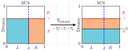
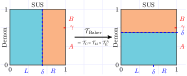
(a)                                                                        (b)

Figure S1: Dynamical Szilard Engine Composite Maps: (a) Szilard Map $\mathcal{T}_{\mathrm{Szilard}}=\mathcal{T}_{\mathrm{Erase}}^{A}\circ\mathcal{T}_{\mathrm{Control}}\circ\mathcal{T}_{\mathrm{Measure}}$ and (b) Asymmetric Baker’s Map $\mathcal{T}_{\mathrm{Baker}}=\mathcal{T}_{\mathrm{Control}}\circ\mathcal{T}_{\mathrm{Measure}}\circ\mathcal{T}_{\mathrm{Erase}}^{A}$. These assume the Demon’s reset memory state is $A$. Areas left and right of $\delta$ are colored only as an aid to understanding the maps’ action and to track the particle location history.

II Szilard Engine Dynamical System: An Animation

Probably the most direct way to understand the operation of Szilard’s Engine is via a continuous-time embedding of $\mathcal{T}_{\mathrm{Szilard}}$. Animations can be viewed at http://csc.ucdavis.edu/~cmg/compmech/pubs/dds.htm.

Here, we provide accompanying descriptive text that addresses several issues: How the discrete-time $\mathcal{T}_{\mathrm{Szilard}}$ is embedded in continuous time, what the protocol cycle looks like in operation, where the instability and chaos occur (during energy extraction), what erasure affects, and, notably, the appearance of self-similar (fractal) structure in the joint state-space distribution.

Background:

In 1929 Szilard Futz_Szil29a gave Maxwell’s Demon its first logical resolution—that “intelligence” was not violating the Second Law—by accounting for the Demon’s own, what we now call, information processing:

…we must conclude that the intervention which establishes the coupling between $y$ and $x$, the measurement of $x$ by $y$, must be accompanied by a production of entropy.

(Cf. Smoluchowski’s “physical” resolution Smol12a,Smol14a,Feyn63a.)

Szilard Engine Operation:

There are two ways to describe the Engine’s operation: as its action on a single particle or that on an infinite ensemble of particles via evolving a probability density. The graphics and animations show the latter. The former is easier to describe, initially.

Consider a single particle in a box, whose position the Demon determines by placing a partition at $x=\delta$. Then, noting on which side (left or right) the particle falls, the Demon lets the particle push the partition (right or left, respectively) to extract energy ($\int_{\delta}^{1}P~{}dV$ or $\int_{\delta}^{0}P~{}dV$, respectively). (See Sec. V for the thermodynamic calculations.) The entire system is held at constant temperature $T$ by a heat bath. Finally, the Demon’s memory is reset to its original state (mesostate $A$ or $B$).

Our construction of $\mathcal{T}_{\mathrm{Szilard}}$ demonstrates that Szilard’s Engine is, in fact, a deterministic chaotic map of the unit square $\mathbb{I}^{2}=[0,1]\times[0,1]$. The construction “symmetrizes” the Demon and System Under Study (SUS). (The latter is the name for the particle-in-a-box thermodynamic subsystem.) That is, we look at the joint state-space of both the Demon and SUS.

Interpretation:

In the ensemble view, information processing describes changes in the support and shape of the joint state-space distributions. The thermodynamics describes the energy flow to/from the heat bath during each protocol step.

Animation:

This is a continuous-time embedding of the 2D map. Suspending a discrete-time map in a continuous-time flow is a standard, if somewhat under-utilized, visualization technique Maye87a.

The animation shows the evolution of the Engine state-space distribution, beginning when the Demon starts in its “reset” mesostate $A$. Two pieces of the distribution are colored to correspond to the particle in the left or right side of the partition placed at $x=\delta$. This is an aid to visually track the particle’s location and also to highlight the component maps’ actions on areas.

The animation steps through the protocol (i) Measurement (Demon memory state and particle location come into correlation), (ii) Control (extract energy from heat bath), and (iii) Erase (clear Demon memory to start the cycle anew).

The parameter $\gamma\in[0,1]$ represents the division between Demon memory mesostates $A$ and $B$.

$\gamma$ and $\delta$ together let us explore the “efficiency” of Demon measurements of particle location.

The energy extraction (“gas expansion”) corresponds to the state-space stretching during the thermodynamic control step $\mathcal{T}_{\mathrm{C}}$. This is particularly noteworthy: The instability of chaos is essential to energy extraction.

Crucially, one sees another consequence of the chaotic dynamics: The build-up over each cycle of the self-similar (fractal) structure of the joint state-space distribution.

The construction allows one to make a solid connection between thermodynamics, information processing, and chaotic dynamics. Indeed, everything can be analytically calculated. Leaving few, if any, remaining mysteries for the Szilard Engine, as originally conceived. In this light, Szilard’s conclusion takes on new meaning Futz_Szil29a:

…a simple inanimate device can achieve the same essential result as would be achieved by the intervention of intelligent beings. We have examined the “biological phenomena” of a nonliving device and have seen that it generates exactly that quantity of entropy which is required by thermodynamics.

With this firm foundation, designing and analyzing more sophisticated thermodynamic control systems becomes possible, including monitoring information creation and the necessary attributes of “intelligence”.

III Spectrum of Lyapunov Characteristic Exponents

The Szilard Map Jacobian $\partial_{xy}\mathcal{T}_{\mathrm{Szilard}}$ determines its local linearization and so one can easily calculate the spectrum of Lyapunov characteristic exponents (LCEs) for each thermodynamic step and for the overall cycle [15, 16]. This gives insight into the directions (submanifolds) of stability (convergence) and instability (divergence). We work with $\mathcal{T}_{\mathrm{Baker}}$. There are two LCEs. We find that one is positive:

$$\lambda^{+} =\lim_{t\to\infty}t^{-1}\log_{2}\big{|}\partial_{xy}\mathcal{T}_{\mathrm{Baker}}^{t}(x_{0},y_{0})\cdot\delta\vec{x}\big{|}~{},$$

where, since the unstable manifolds parallel the $x$-axis, the initial vector is $\delta\vec{x}=(1,0)$. Due to ergodicity, we can calculate via:

$$\lambda^{+} =\int_{0}^{1}dx\left[\int_{0}^{\delta}dy~{}\widehat{\rho}~{}\log_{2}\delta+\int_{\delta}^{1}dy~{}\widehat{\rho}~{}\log_{2}(1-\delta)\right]$$

$$=\operatorname{H}(\delta)~{}.$$

There is no dependence on initial condition $(x_{0},y_{0})\in\mathbb{I}^{2}$. There is a companion negative LCE that monitors state space contraction. Since the stable manifolds parallel the $y$-axis, we take the initial vector $\delta\vec{y}=(0,1)$, finding:

$$\lambda^{-} =\lim_{t\to\infty}t^{-1}\log_{2}\big{|}\partial_{xy}\mathcal{T}_{\mathrm{Baker}}^{t}(x_{0},y_{0})\cdot\delta\vec{y}\big{|}$$

$$=-\operatorname{H}(\delta)~{}.$$

Note that state-space area preservation is reflected in the exact balance of instability and stability: $\lambda^{+}+\lambda^{-}=0$. More specifically, the unstable manifold supports the mechanism that amplifies small fluctuations from the heat bath to macroscopic scale and so to extractable work. The stable manifold is the mechanism that dissipates energy into the ambient heat bath, due to Demon memory resetting.

IV Intrinsic Computation Calculations

We can project the global symbolic dynamics, captured by the $\epsilon$-transducer of Fig. 2(a), onto just that for the Demon (over alphabet $\{A,B\}$) or just that for the SUS (over alphabet $\{L,R\}$). The SUS and Demon $\epsilon$-transducers are shown in Fig. S2(a) and S2(b), respectively. Comparisons are insightful.

The projections make it clear that the SUS and Demon $\epsilon$-transducers are duals of each other. When one splits into multiple causal states, the other contracts its causal states, as expected. Branching and contraction must be balanced in a state-space volume preserving system.

Computational mechanics analysis shows that the SUS system has an entropy rate of:

$$h_{\mu}^{\text{SUS}} =\operatorname{H}[X|\mathcal{S}]$$

$$=-\sum_{\sigma\in\bm{\mathcal{S}}^{\text{SUS}}}\Pr(\sigma)\sum_{x\in\{L,R\}}\Pr(x|\sigma)\log_{2}\Pr(x|\sigma)$$

$$=\operatorname{H}(\delta)/3~{},$$

where $\bm{\mathcal{S}}^{\text{SUS}}$ is the set of its causal states, and a statistical complexity of:

$$C_{\mu}^{\text{SUS}} =\operatorname{H}[\Pr(\mathcal{S})]$$

$$=-\sum_{\sigma\in\bm{\mathcal{S}}^{\text{SUS}}}\Pr(\sigma)\Pr(\sigma)\log_{2}\Pr(\sigma)$$

$$=\log_{2}3+2/3\operatorname{H}(\delta)~{}.$$

Note that the time scale here is measured in individual protocol steps.

The Demon’s memory process has the same entropy rate $h_{\mu}^{\text{Demon}}=\operatorname{H}(\delta)/3$, but different statistical complexity $C_{\mu}^{\text{Demon}}=\log_{2}3+1/3\operatorname{H}(\delta)$. For the overall Szilard information engine (Fig. 2(a)) we find that it has the same entropy rate $h_{\mu}^{\text{Szilard}}=\operatorname{H}(\delta)/3$, but statistical complexity $C_{\mu}^{\text{Szilard}}=\log_{2}3+\operatorname{H}(\delta)$. The analysis shows us that the SUS and the Demon subsystems are not independent, however. The joint $C_{\mu}^{\text{Szilard}}$ is substantially less than the sum of that of the two subsystems: $C_{\mu}^{\text{Szilard}}=C_{\mu}^{\text{SUS}}+C_{\mu}^{\text{Demon}}-\log_{2}3$. Not surprisingly, the two subsystems are redundant in their operation. The $\log_{2}3$ bits of memory reflect the synchronization of SUS and Demon during the period-$3$ control protocol, which is accounted for only once in the overall Engine $C_{\mu}^{\text{Szilard}}$.

An information engine is a control system and its effectiveness depends on the controller (Demon) knowing the state of the thermodynamic subsystem (SUS). So, how predictable is the SUS from the Demon’s perspective? And, for that matter, since our construction is symmetrized, the Demon from the viewpoint of the SUS? The answers start with the information engine’s past-future mutual information, the excess entropy: ${\bf E}^{\text{Szilard}}=\operatorname{I}[\smash{\overleftarrow{Z}};\smash{\overrightarrow{Z}}]$, where $\smash{\overleftarrow{Z}}=\ldots Z_{-3}Z_{-2}Z_{-1}$ is the past and $\smash{\overrightarrow{Z}}=Z_{0}Z_{1}Z_{2}\ldots$ is the future of the joint process over random variable $Z_{t}\in\{A,B\}\otimes\{R,L\}$. ${\bf E}^{\text{Szilard}}$ measures the amount of future information predictable from the past. We can also ask about the predictability of the individual SUS and Demon subprocesses using ${\bf E}^{\text{SUS}}$ and ${\bf E}^{\text{Demon}}$, respectively, defined similarly. We see that the machines in Fig. S2 are counifilar Crut08a,Crut08b and so ${\bf E}^{\text{Szilard}}=C_{\mu}^{\text{Szilard}}$, ${\bf E}^{\text{Demon}}=C_{\mu}^{\text{Demon}}$, and ${\bf E}^{\text{SUS}}=C_{\mu}^{\text{SUS}}$ Crut08b. (Section VI calculates the inter-subsystem information flows.)

(a) SUS $\epsilon$-transducer.                 (b) Demon $\epsilon$-transducer.

Figure S2: $\epsilon$-Transducers for the symbolic dynamics of the Szilard information engine from the Markov partition of the Demon and SUS state spaces: (a) $\epsilon$-Transducer for the thermodynamic system, giving the $\{R,L\}$-symbolic dynamics of particle location when the engine’s $\epsilon$-transducer is driven by the period-$3$ measurement protocol: $M\to C\to E\to\ldots$. (b) $\epsilon$-Transducer for the Demon’s memory, with the engine similarly driven. $\epsilon$-Transducer transitions $\beta|\alpha:p$ denote taking a transition with probability $p$ on seeing $\alpha=\{M,E,C\}$ and emitting symbol $\beta\in\{R,L\}$ or $\beta\in\{A,B\}$. Asymptotic state probabilities are given in parentheses underneath state names.

V Engine Thermodynamics

The minimum energy cost of the measurement, control, and erasure protocol steps can be calculated by treating the Szilard Engine as a box of ideal gas. (Sequels address more realistic models of the working fluid.) Each of the transitions shown in Fig. 1 is achieved by isothermal sliding of barriers, so the work done is exactly calculable by integrating the force on these barriers. The work done on this system is equal to the heat dissipated, since the thermal energy of the particle does not change for an isothermal process.

For each component-map thermodynamic transformation, the work done on the system is given by $W=-\int PdV$, where $P=k_{B}T/V$ for a single particle. Thus:

$$W=-\int_{V_{0}}^{V_{1}}\frac{k_{B}T}{V}dV=k_{B}T\ln\frac{V_{0}}{V_{1}}~{},$$

where $V_{0}$ is the initial volume of the region being manipulated and $V_{1}$ is the final volume.

Assume the Demon resets to mesostate $A$.

To calculate the thermodynamic cost of measurement $\langle Q_{\mathrm{measure}}\rangle$, note that there are two regions where the particle can exist. The particle starts in a uniform distribution over the $L\otimes A$ and $R\otimes A$ regions. The probability of being in each of those regions is proportional to the the region’s volume. Assuming the box has volume $V$, the size of region $L\otimes A$ is $\delta\gamma V$ and the size of region $R\otimes A$ is $(1-\delta)\gamma V$. Thus, before measurement, the probability of being in $R\otimes A$ is $(1-\delta)$.

The region $L\otimes A$ is unchanged under the measurement map $\mathcal{T}_{\mathrm{M}}$, meaning that there is no work done in the case where the particle is on the left. However, if the particle is on the right, volume is being moved to the $R\otimes B$ region, so we have a change in volume. The resulting average work done is the average dissipated heat:

$$\langle Q_{\mathrm{measure}}\rangle =\langle W_{\text{measure}}\rangle$$

$$=\Pr(L\otimes A)\times 0+\Pr(R\otimes A)\times-\int_{V_{R\otimes A}}^{V_{R\otimes B}}PdV$$

$$=0+(1-\delta)k_{B}T\ln\frac{V_{R\otimes A}}{V_{R\otimes B}}$$

$$=-k_{B}T(1-\delta)\ln\frac{1-\gamma}{\gamma}~{}.$$

Before the thermodynamic control transformation $\mathcal{T}_{\mathrm{C}}$, the particle has probability $\delta$ of being in the $L\otimes A$ region and probability $1-\delta$ of being in the $R\otimes B$ region. If the particle is in the $L\otimes A$ region, then after control the particle occupies the whole $A$ region, and if it was in $R\otimes B$, then it occupies the whole $B$ region. According to the change in volume, the average heat dissipated is:

$$\langle Q_{\mathrm{control}}\rangle =\langle W_{\text{control}}\rangle$$

$$=-\Pr(L\otimes A)\int_{V_{L\otimes A}}^{V_{L\otimes A}+V_{R\otimes A}}\frac{k_{B}T}{V}dV-\Pr(R\otimes B)\int_{V_{R\otimes B}}^{V_{R\otimes B}+V_{L\otimes B}}\frac{k_{B}T}{V}dV$$

$$=-\delta k_{B}T\ln\frac{V\gamma}{V\delta\gamma}-(1-\delta)k_{B}T\ln\frac{V(1-\gamma)}{V(1-\delta)(1-\gamma)}$$

$$=-k_{B}T(-\delta\ln\delta-(1-\delta)\ln(1-\delta))$$

$$=-k_{B}T\ln 2\,\operatorname{H}(\delta)~{}.$$

Before the erasure transformation $\mathcal{T}_{\mathrm{E}}$, the particle has probability $\delta$ of being distributed uniformly over the $A$ region and probability $1-\delta$ of being distributed uniformly over the $B$ region. The $B$ region is compressed into the region between $\eta=\gamma\delta$ and $\gamma$ on the vertical demon axis, which has volume $\gamma(1-\delta)V$. The $A$ region is compressed between $0$ and $\eta$ on the Demon axis, which has volume $\gamma\delta V$. The associated heat dissipation is, then:

$$\langle Q_{\mathrm{erase}}\rangle =\langle W_{\text{erase}}\rangle$$

$$=-\Pr(B)\int_{(1-\gamma)V}^{\gamma(1-\delta)V}\frac{k_{B}T}{V}dV-\Pr(A)\int_{\gamma V}^{\gamma\delta V}\frac{k_{B}T}{V}dV$$

$$=-k_{B}T((1-\delta)\ln\frac{\gamma(1-\delta)}{1-\gamma}+\delta\ln\delta)$$

$$=k_{B}T\ln 2\,\operatorname{H}(\delta)+k_{B}T(1-\delta)\ln\frac{1-\gamma}{\gamma}~{}.$$

After erasure, the particle is once again uniformly distributed over the $A$ region.

We close by commenting on the main text’s mention of the Szilard Engine’s optimality. We note that the results above match those in Ref. Saga12a for $\delta=1/2$. Moreover, they achieve the bounds described there for all $\delta$ and $\gamma$. Specifically, for $\delta=1/2$, our results match Eq. (7.23) for erasure and Eq. (7.40) for measurement. And, our results achieve the lower bounds given there in Eqs. (7.41), (7.43), and (7.44), since $I_{QC}=H(\delta)$. Our development, though, places measurement, control, and erasure on the same footing, allowing us to make the same statements about each, which is that we quantify how much heat they dissipate.

VI Monitoring Correlation and Coordination During the Control Protocol

There are many different correlations potentially relevant to Demon functioning and to monitoring its interaction with the SUS. Let $Y$ be the random variable for the Demon’s memory $\{A,B\}$. Let $X$ be the random variable for the SUS’s particle locations $\{L,R\}$. Let $S^{Y}$ be that for Demon’s causal states (Fig. S2(b)) and $S^{X}$ that for SUS’s causal states (Fig. S2(a)).

The first mutual information we consider is the asymptotic communication rate between the Demon and the SUS:

$$\lim_{\ell\rightarrow\infty}\frac{\operatorname{I}[X_{0:\ell};Y_{0:\ell}]}{\ell}~{},$$ (S1)

where the random variable blocks are $X_{0:\ell}=X_{0}X_{1}\ldots X_{\ell-1}$ and $Y_{0:\ell}=Y_{0}Y_{1}\ldots Y_{\ell-1}$. This can be evaluated by breaking it into components:

$$\lim_{\ell\rightarrow\infty}\frac{\operatorname{I}[X_{0:\ell};Y_{0:\ell}]}{\ell} =\lim_{\ell\rightarrow\infty}\frac{1}{\ell}\left(\operatorname{H}[X_{0:\ell}]+\operatorname{H}[Y_{0:\ell}]-\operatorname{H}[X_{0:\ell},Y_{0:\ell}]\right)$$

$$=h_{\mu}[\overleftrightarrow{X}]+h_{\mu}[\overleftrightarrow{Y}]-h_{\mu}[\overleftrightarrow{X},\overleftrightarrow{Y}]$$

$$=\operatorname{H}(\delta)/3+\operatorname{H}(\delta)/3-\operatorname{H}(\delta)/3$$

$$=\operatorname{H}(\delta)/3~{}.$$

Note that the Shannon (base 2) binary entropy function $\operatorname{H}(\delta)$ Cove06aSupp features prominently in the expressions for heat dissipation. However, the above shows that it often signifies an amount of shared or mutual information, not just a degree of Shannon information uncertainty. These two interpretations are rather distinct.

This should be compared to single-symbol (length-$1$ block) mutual information between the Demon and SUS:

$$\operatorname{I}[X_{0};Y_{0}] =\frac{\delta(2+\delta)}{3}\log_{2}\frac{2+\delta}{1+\delta}+\frac{(1-\delta)(1+\delta)}{3}\log_{2}\frac{1+\delta}{2+\delta}$$ (S2)

$$\quad-\frac{\delta(1-\delta)}{3}+\frac{(1-\delta)(2-\delta)}{3}\log_{2}\frac{2-\delta}{2-2\delta}~{}.$$ (S3)

Note that this differs from the asymptotic rate above and so the single-symbol quantity misestimates the degree of Demon-SUS correlation.

To measure the degree of internal coordination between the SUS and the Demon, consider now the single-symbol mutual information between the SUS and Demon causal states. First, we find the stationary distribution over the causal states in the joint process (Fig. 2(a)) and label the joint causal states with the corresponding causal states of the SUS and Demon. The resulting single-state mutual information is:

$$\operatorname{I}[S^{X}_{0};S^{Y}_{0}]=\log_{2}3~{}.$$

This tells us the correlation between SUS and Demon causal states is limited to their synchronization within the three step cycle of measurement, control, and erasure.

We can similarly calculate the correlation rate between the Demon and SUS states. For this we need the $\epsilon$-transducers for the joint, Demon, and SUS processes in Figs. 2(a), S2(a), and S2(b), respectively. It turns out that the entropy rate for all three machines is also $\operatorname{H}(\delta)/3$ as well, so:

$$\lim_{\ell\rightarrow\infty}\frac{\operatorname{I}[S^{X}_{0:\ell};S^{Y}_{0:\ell}]}{\ell} =\operatorname{H}(\delta)/3+\operatorname{H}(\delta)/3-\operatorname{H}(\delta)/3$$

$$=\operatorname{H}(\delta)/3~{}.$$

This equals the communication rate between the Demon and SUS symbolic processes above, indicating that there is little “hidden” internal state information compared to the symbolic processes. The Szilard Engine is not a cryptic process Crut08a.

Last, adopting the transducer perspective, we calculate the single-symbol conditional mutual information between the Demon and SUS variables given the three possible control protocol inputs. These monitor the dependence of correlation during the individual protocol steps. Let our input control variable be $Z$ over alphabet $\{M,C,E\}$. For instance, during the measurement step, we directly calculate:

$$\operatorname{I}[X_{0};Y_{0}|Z_{0}=M] =\sum_{y\in\{A,B\}}\sum_{x\in\{L,R\}}\Pr(X_{0}=x,Y_{0}=y|Z_{0}=M)\log_{2}\left(\frac{\Pr(X_{0}=x,Y_{0}=y|Z_{0}=M)}{\Pr(X_{0}=x|Z_{0}=M)\Pr(Y_{0}=y|Z_{0}=M)}\right)$$

$$=\operatorname{H}(\delta)~{}.$$

Similarly, we calculate that during erasure there is no correlation:

$$\operatorname{I}[X_{0};Y_{0}|Z_{0}=E]=0~{},$$

and that during thermodynamic control the same holds true:

$$\operatorname{I}[X_{0};Y_{0}|Z_{0}=C]=0~{}.$$

Thus, the single-symbol correlation between Demon and SUS comes from measurement. There is also a connection between these quantities and the work extracted during control. The work extracted in control is $\braket{W}=k_{B}T\operatorname{H}(\delta)\ln 2$. That is, the Engine uses the decrease in correlation of mesostates between measurement and control to extract work from the thermal bath.

Note that these calculations for the Szilard Engine are straightforward. We detail them here to show the individual analyses, uncluttered by distracting calculational moves, that one must do for more complex information engines. In the latter cases, especially when the thermodynamical system is nonhyperbolic, the calculations can be quite challenging. Sequels illustrate.

chaos

References

- [1] T. Rueckes, K. Kim, E. Joselevich, Greg Y. Tseng, C-L. Cheung, and C. M. Lieber. Science, 289:94–97, 2000.
- [2] A. M. Fennimore, T. D. Yuzvinsky, W.-Q. Han, M. S. Fuhrer, J. Cumings, and A. Zettl. Nature, 424:408–410, 2003.
- [3] Z. Zhong, D. Wang, Y. Cui, M. W. Bockrath, and C. M. Lieber. Science, 302:1377–1379, 2003.
- [4] J. Chen, N. Jonoska, and G. Rozenberg, editors. Nanotechnology: Science and Computation, Natural Computing, New York, 2006. Springer-Verlag.
- [5] F. Julicher, A. Ajdari, and J. Prost. Rev. Mod. Phys., 69(4):1269–1281, 1997.
- [6] C. Bustamante, J. Liphardt, and F. Ritort. Physics Today, 58(7):43–48, 2005.
- [7] A. R. Dunn and A. Price. Physics Today, 68(2):27–32, 2015.
- [8] L. Zhuang, L. Guo, and S. Y. Chou. Appl. Phys. Lett., 72(10):1205–1207, 1998.
- [9] F. Hetsch, N. Zhao, S. V. Kershaw, and A. L. Rogach. Materials Today, 16(9):312–325, 2013.
- [10] S. Toyabe, T. Sagawa, M. Ueda, E. Muneyuki, and M. Sano. Nature Physics, 6:988–992, 2010.
- [11] A. Berut, A. Arakelyan, A. Petrosyan, S. Ciliberto, R. Dillenschneider, and E. Lutz. Nature, 483:187–190, 2012.
- [12] R. Klages, W. Just, and C. Jarzynski, editors. Wiley, New York, 2013.
- [13] L. Szilard. Z. Phys., 53:840–856, 1929.
- [14] Cf. the schematic diagram in Ref. [23, Fig. 12], a more complicated product system, used to argue that only erasure during logically irreversible operations dissipates energy. This, however, is a restricted case.
- [15] A. Lasota and M. C. Mackey. Probabilistic Properties of Deterministic Systems. Cambridge University press, Cambridge, United Kingdom, 1985.
- [16] J. R. Dorfman. An Introduction to Chaos in Nonequilibrium Statistical Mechanics. Cambridge University Press, Cambridge, United Kingdom, 1999.
- [17] T. M. Cover and J. A. Thomas. Elements of Information Theory. Wiley-Interscience, New York, second edition, 2006.
- [18] Ja. G. Sinai. Dokl. Akad. Nauk. SSSR, 124:768, 1959.
- [19] J. P. Crutchfield. Nature Physics, 8(January):17–24, 2012.
- [20] N. Barnett and J. P. Crutchfield. J. Stat. Phys., to appear, 2015.
- [21] C. J. Ellison, J. R. Mahoney, and J. P. Crutchfield. J. Stat. Phys., 136(6):1005–1034, 2009.
- [22] R. Landauer. IBM J. Res. Develop., 5(3):183–191, 1961.
- [23] C. H. Bennett. Intl. J. Theo. Phys., 21:905, 1982.
- [24] K. Shizume. Phys. Rev. E, 52(4):3495–3499, 1995.
- [25] F. N. Fahn. Found. Physics, 26(1):71–93, 1996.
- [26] M. M. Barkeshli. arXiv:cond-mat, 0504323.
- [27] T. Sagawa. Prog. Theo. Phys., 127, 2012.
- [28] D. Mandal and C. Jarzynski. Proc. Natl. Acad. Sci. USA, 109(29):11641–11645, 2012.