Polynomial Bell inequalities

Abstract

It is a recent realization that many of the concepts and tools of causal discovery in machine learning are highly relevant to problems in quantum information, in particular quantum nonlocality. The crucial ingredient in the connection between both fields is the tool of Bayesian networks, a graphical model used to reason about probabilistic causation. Indeed, Bell’s theorem concerns a particular kind of a Bayesian network and Bell inequalities are a special case of linear constraints following from such models. It is thus natural to look for generalized Bell scenarios involving more complex Bayesian networks. The problem, however, relies on the fact that such generalized scenarios are characterized by polynomial Bell inequalities and no current method is available to derive them beyond very simple cases. In this work, we make a significant step in that direction, providing a general and practical method for the derivation of polynomial Bell inequalities in a wide class of scenarios, applying it to a few cases of interest. We also show how our construction naturally gives rise to a notion of nonsignalling in generalized networks.

Bell’s theorem Bell (1964) demonstrates that our classical conceptions of causal relations must be taken with care, as they fail to commit with the results obtained in some quantum experiments performed by distant parties, the phenomenon known as quantum nonlocality. Even without detailed information about the underlying processes, the causal structure of the setup alone already implies strong constraints – the famous Bell’s inequalities – on the correlations that are compatible with it.

This is close to the reasoning employed in the field of causal inference Pearl (2009); Spirtes et al. (2001), a connection that has recently attracted considerable attention Ver Steeg and Galstyan (2011); Fritz (2012, 2014); Chaves et al. (2014a); Wood and Spekkens (2015); Henson et al. (2014); Chaves et al. (2015a, b); Ried et al. (2015). Since Bell’s theorem is a statement about classical correlations, it comes as no surprise that mathematical tools and concepts, originally devised in a causal inference context, can also be applied to the study of nonlocality. Indeed, Bell’s theorem concerns the same kind of causal structures that are the object of study in Bayesian networks Pearl (2009) and Bell inequalities are a special case of linear constraints following from such models Ver Steeg and Galstyan (2011). Bayesian networks not only offer a new conceptual perspective to revisit quantum nonlocality Wood and Spekkens (2015); Chaves et al. (2015b) but also provide the right language to devise generalized Bell scenarios Fritz (2012, 2014).

Several extensions of the paradigmatic Bell experiment – two distant parties, performing two possible experiments on their shares of a joint system – have been proposed, including more parties Werner and Wolf (2001); Zukowski and Brukner (2002), more measurements/outcomes Collins et al. (2002); Collins and Gisin (2004) and sequential measurements Popescu (1995); Gallego et al. (2014). However, all these different generalizations share the same basic property: the correlations between all the parties originate from a single (not directly observable) source, being therefore named as local hidden variable (LHV) models. In spite of the rich plethora of phenomena and applications Brunner et al. (2014), LHV models represent a very particular case of the possibilities offered by Bayesian networks. Those typically include several independent hidden variables and will be named here as generalized local hidden variable (GLHV) models. These scenarios with many independent sources are also ubiquitous in quantum information, e.g., entanglement percolation Acín et al. (2007), entanglement swapping Zukowski et al. (1993) and quantum repeaters Sangouard et al. (2011); Sen (De). Thus, understanding generalized Bell scenarios is not only of fundamental interest but also of high practical relevance.

Within that context, the basic question to be solved is how to derive Bell inequalities for general Bayesian networks. Bell inequalities play a fundamental role in study of nonlocality, since it is via their violation (e.g. with quantum entangled states) that we can witness the nonlocal character of a given experimental data. Unfortunately, as opposed to usual Bell scenarios, a GLHV model implies a non-convex region – characterized by polynomial Bell inequalities – of correlations that are compatible with it. Generally, algebraic geometry methods can be used to characterize such polynomial constraints Geiger and Meek (1999); Garcia et al. (2005), but given their computational complexity, in practice they are intractable even for very simple models Ver Steeg and Galstyan (2011). Arguably, because of this difficulty, only sparse results have been obtained in the derivation of Bell inequalities for GLHV models, either using coarse-grained information Steudel and Ay (2015); Chaves and Fritz (2012); Fritz (2012); Chaves et al. (2014b); Henson et al. (2014) or considering particular scenarios Branciard et al. (2010, 2012); Tavakoli et al. (2014); Mukherjee et al. (2014). However, to our knowledge, no practical and systematic method for the derivation of polynomial Bell inequalities for GLHV models is known to this date.

In this paper we propose a general method for deriving polynomial Bell inequalities in a wide class of Bayesian networks. In spite of the non-convex character of the problem, we show how to obtain polynomial inequalities resorting to a linear programming technique, namely a Fourier-Motzkin elimination Williams (1986). We illustrate the general method applying it to a few relevant cases and derive new polynomial Bell inequalities. Furthermore, we explain how our construction naturally leads to a notion of nonsignalling correlations Popescu and Rohrlich (1994) in generalized Bell networks.

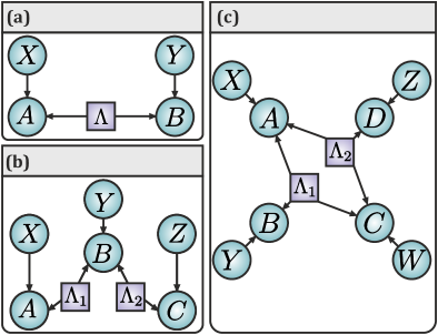
Figure 1: DAG representation of Bayesian networks. (a) Bipartite LHV model. (b) GLHV model with $2$ independent hidden variables representing the bilocality scenario of Branciard et al. (2010). (c) GLHV model with $2$ hidden variables shared among $4$ parties.

I Bell inequalities, Bayesian networks and marginal problems

Bell scenarios beyond LHV models can be represented via the graphical notation of Bayesian networks Pearl (2009); Spirtes et al. (2001). Underlying models are represented by directed acyclic graphs (DAG), where nodes stand for variables and directed arrows represent their causal relations Pearl (2009). While LHV models correspond to a DAG with a single hidden variable (see Fig. 1(a)), GLHV models are represented by DAGs with $n\geq 2$ independent hidden variables (see Fig. 1(b)-(c)). The causal relations implied by a DAG are captured by the (conditional) independencies (CI) implied by the graph and that can be listed by the d-separation criterion Pearl (2009). For instance, for the LHV model in Fig. 1(a) it follows that $p(x,y,\lambda)=p(x)p(y)p(\lambda)$ and $p(a|x,y,\lambda)=p(a|x,\lambda)$ (similarly to $b$). Thus, any observable data – given by the probability distribution $p(a,b|x,y)$ – compatible with this LHV model can be decomposed as

$$p(a,b|x,y)=\sum_{\lambda}p(a|x,\lambda)p(b|y,\lambda)p(\lambda).$$ (1)

That is, any local distribution must lie inside the convex set defined by (1), the so-called correlation polytope $\mathbb{C}$ Pitowsky (1989, 1991). In this geometric picture, (linear) Bell inequalities are nothing else than facets of $\mathbb{C}$. Given that it is easy to list the extremal points of $\mathbb{C}$, to find its facets amounts to an efficient linear program, arguably the reason why this method has become the most prominent in the study of nonlocality.

Another equivalent, but far less used method, comes from the realization that Bell inequalities are constraints arising from a marginal problem Budroni and Cabello (2012); Fritz and Chaves (2013); Kurzyński and Kaszlikowski (2014), that can be stated as: given some marginal distributions of $n$ variables is it possible to find a joint distribution of all variables, such that this distribution marginalizes to the given ones? To see that Bell’s theorem is indeed a particular marginal problem, notice that the LHV description (1) is equivalent to the existence of a joint distribution $\mathbf{p}=p(a_{0},\dots,a_{m_{x}},b_{0},\dots,b_{m_{y}})$ (represented as a vector $\mathbf{p}$) describing the probability for outcomes of all possible measurements, where $a_{i}$ labels the outcome $a$ given that $x=i=\left\{0,\dots,m_{x}\right\}$ and similarly for $b$. Since $\mathbf{p}$ defines a valid probability, it is constrained by a set of linear inequalities $L\mathbf{p}\geq 0$ given by $p_{i}\geq 0$ (positivity) and $\sum_{i}p_{i}=1$ (normalization) defining the simplex polytope $\mathbb{P}$ Boyd and Vandenberghe (2009). Given that at each round of the experiment only one $a_{i}$ and one $b_{j}$ can be measured simultaneously, $\mathbf{p}$ defines a non-observable quantity. However, the constraints on $\mathbf{p}$ will also imply constraints on the level of the observable distributions $p(a_{i},b_{j})$. These are exactly Bell inequalities, that in this picture can be understood as a condition for the marginal problem to have a positive answer. Thus, to obtain Bell inequalities in this picture, we have to eliminate from our description all non-observable terms. This is a achieved via a FM elimination Williams (1986), a standard algorithm for the elimination of variables from a system of inequalities.

For simplicity and without loss of generality, in the remaining of the paper we focus on dichotomic outcomes (e.g. $a_{i}=0,1$). It is then convenient to consider the equivalent description of the problem in terms of the correlation vector $\mathbf{E}$ with components given by expectation values, e.g., $\langle A_{i}B_{j}\rangle=\sum_{a_{i},b_{j}}(-1)^{a_{i}+b_{j}}p(a_{i},b_{j})$. The vectors $\mathbf{E}$ and $\mathbf{p}$ are linearly related as $\mathbf{E}=T^{-1}\mathbf{p}$ implying that $\mathbf{E}$ must obey linear inequalities $T\mathbf{E}\geq 0$ plus a normalization constraint. To illustrate the FM elimination consider the CHSH scenario Clauser et al. (1969) where each of the two parties in Fig. 1(a) can measure two observables. The inequalities

$$\langle A_{0}B_{0}\rangle+\langle A_{1}B_{0}\rangle-\langle A_{0}A_{1}\rangle\leq 1,$$ (2)

$$\langle A_{0}B_{1}\rangle-\langle A_{1}B_{1}\rangle+\langle A_{0}A_{1}\rangle\leq 1,$$ (3)

directly follow from $T\mathbf{E}\geq 0$ after the elimination of terms like $\langle A_{0}A_{1}B_{0}B_{1}\rangle$ and $\langle A_{0}A_{1}B_{0}\rangle$. The sum of (2) and (3) eliminates the remaining non-observable term $\langle A_{0}A_{1}\rangle$ leading exactly to the CHSH inequality Clauser et al. (1969).

II Polynomial Bell inequalities

Similarly to LHV models, a GLHV model also implies the existence of a well defined a joint distribution $\mathbf{p}$ characterized by linear inequalities $L\mathbf{p}\geq 0$. The difference resides on the fact that GLHV models also imply a set of non-linear inequalities $W\mathbf{p}\geq 0$ (where $W=W(\mathbf{p})$). Thus, a GLHV model is characterized by intersection of $\mathbb{P}$ with $W\mathbf{p}\geq 0$, that is, a semi–algebraic set Geiger and Meek (1999). As discussed before, this system of inequalities involves non-observable quantities that have to be eliminated in order to obtain a description in terms of empirically accessible variables only. Formally, the problem at hand is equivalent to a quantifier elimination: the projection of a semi–algebraic set onto a subspace of it, that by Tarski-Seidenberg theorem is again guaranteed to be a semi–algebraic set Geiger and Meek (1999). In other terms, the correlations compatible with a GLHV model are characterized by finitely many polynomial Bell inequalities. Quantifier elimination is routinely encountered in algebraic geometry problems, thus general purpose methods have been developed Geiger and Meek (1999). Unfortunately, given their computational complexity, their application to Bell scenarios is intractable even for the simplest possible models Ver Steeg and Galstyan (2011). Notwithstanding, we show next that a simple adaptation of the FM elimination leads to practical and computational tractable way for deriving polynomial Bell inequalities.

The class of DAGs we consider are those which display (conditional) independencies on the level of the joint distribution $\mathbf{p}$. This is the case, for instance, in the DAG of Fig. 1(b) implying the independence relation $p(a,c)=p(a)p(c)$ and for many other relevant scenarios in quantum information Zukowski et al. (1993); Sen (De); Acín et al. (2007); Branciard et al. (2010); Fritz (2012); Tavakoli et al. (2014); Mukherjee et al. (2014). The method to derive polynomial inequalities for this class of scenarios proceed as follows.

Given $\mathbf{p}$ we first need to list all its components that are to be eliminated from our description: $\mathbf{p}_{\mathrm{O}}$ and $\mathbf{p}_{\mathrm{NO}}$ stand, respectively, to the set of observable and non-observable (to be eliminated) components $p_{i}$. We also list all the terms in $\mathbf{p}_{\mathrm{NO}}$ appearing in a non-linear fashion in $W\mathbf{p}\geq 0$, labeled by $\mathbf{p}_{\mathrm{WNO}}$. Notice that all terms appearing in $\mathbf{p}_{\mathrm{NO}}$ but not in $\mathbf{p}_{\mathrm{WNO}}$ can be eliminated via a usual FM elimination over $L\mathbf{p}\geq 0$, obtaining a new set of linear relations $L^{\prime}\mathbf{p}\geq 0$. The terms in $\mathbf{p}_{\mathrm{WNO}}$ have to be eliminated considering $L^{\prime}\mathbf{p}\geq 0$ and $W\mathbf{p}\geq 0$ jointly. To that aim, notice that $W\mathbf{p}\geq 0$ can be linearized by considering some of the variables as free parameters of the problem. Given $W\mathbf{p}\geq 0$ there is going to be a minimum set of variables $\mathbf{p}^{\prime}_{\mathrm{WNO}}$ that need to be set to free parameters in order to linearize the problem. This means that we can apply a FM elimination to the remaining terms obtaining a final set of inequalities that will depend linearly on the observable terms $\mathbf{p}_{\mathrm{O}}$ and polynomially on terms $\mathbf{p}^{\prime}_{\mathrm{WNO}}$. The observable data will also imply linear constraints on the parameters $\mathbf{p}^{\prime}_{\mathrm{WNO}}$. Together with these constraints, the obtained polynomials can be further simplified by usual quantifier elimination methods, finally arriving at polynomial inequalities involving observable data only. We highlight that following this procedure, one can derive all polynomial Bell inequalities following from the intersection of $L\mathbf{p}\geq 0$ and $W\mathbf{p}\geq 0$, that is, our method provides a full characterization of the GLHV models under consideration. In practice, however, a partial characterization (e.g. in terms of full correlators only) will often be the only computationally tractable approach.

To illustrate the general method, we start considering the bilocality scenario, one of few cases for which polynomial Bell inequalities are known Branciard et al. (2010, 2012); Tavakoli et al. (2014). The scenario involves three parties with correlations mediated via two independent sources (see Fig. 1(b)). In the particular case of two dichotomic measurements per party, the following inequality has been proven to hold Branciard et al. (2010, 2012); Tavakoli et al. (2014)

$$\sqrt{|I|}+\sqrt{|J|}\leq 2,$$ (4)

where $I=\sum_{x,z=0,1}\left\langle A_{x}B_{0}C_{z}\right\rangle$ and $J=\sum_{x,z=0,1}(-1)^{x+z}\left\langle A_{x}B_{1}C_{z}\right\rangle$. However, the methods in Branciard et al. (2012); Tavakoli et al. (2014) cannot be easily generalized to different scenarios, for instance, considering three measurements per party. Next we show in details how our framework can be employed to easily prove (4). We then proceed to derive new polynomial Bell inequalities.

To derive (4), we consider the independence constraint following from the DAG in Fig. 1(b):

$$\left\langle A_{0}A_{1}C_{0}C_{1}\right\rangle=\left\langle A_{0}A_{1}\right\rangle\left\langle C_{0}C_{1}\right\rangle.$$ (5)

We need to combine (5) via a FM elimination with the linear inequalities $T\mathbf{E}\geq 0$. It is sufficient to consider two inequalities following from $T\mathbf{E}\geq 0$:

$$\pm I-\left\langle A_{0}A_{1}\right\rangle-\left\langle C_{0}C_{1}\right\rangle-\left\langle A_{0}A_{1}C_{0}C_{1}\right\rangle\leq 1,$$ (6)

$$\pm J+\left\langle A_{0}A_{1}\right\rangle+\left\langle C_{0}C_{1}\right\rangle-\left\langle A_{0}A_{1}C_{0}C_{1}\right\rangle\leq 1.$$ (7)

Substituting (5) in (6) and (7) and after some algebraic manipulations, we can combine both inequalities into a single polynomial inequality

$$2\left\langle A_{0}A_{1}\right\rangle^{2}+(\pm J\mp I)\left\langle A_{0}A_{1}\right\rangle-(\pm I\pm J+2)\leq 0.$$ (8)

As discussed before, we arrive at an inequality that depends linearly on the observable data (terms $I$ and $J$) but have a non-linear dependence on non-observable terms, in this case $\left\langle A_{0}A_{1}\right\rangle$. The minimum of the polynomial in (8) is achieved at $\left\langle A_{0}A_{1}\right\rangle=(\pm I\mp J)/4$, implying the inequality in terms of observable data only

$$-(1/8)(\pm I-\mp J)^{2}-(\pm I\pm J+2)\leq 0.$$ (9)

This is a quadratic equation that can be easily solved, e.g. for $I$, leading exactly to (4).

Another nice feature of our construction is the fact that independencies are not required to hold exactly. For instance, we may be interested in quantifying how much a given constraint must be relaxed in order to explain some experimental data Hall (2010); Chaves et al. (2015b). In the bilocality scenario if we allow for correlations $\mathcal{C}_{AC}\geq|\left\langle A_{0}A_{1}C_{0}C_{1}\right\rangle-\left\langle A_{0}A_{1}\right\rangle\left\langle C_{0}C_{1}\right\rangle|$ between parts A and C, it follows that

$$-(1/8)(\pm I-\mp J)^{2}-(\pm I\pm J+2)\leq 2\mathcal{C}_{AC},$$ (10)

that is, the violation of (9) quantifies the degree of correlation required to classically reproduce some non-bilocal correlation. As an illustration, consider the correlation $I=J=2$ that can be achieved quantum mechanically with two copies of Bell states shared between the parties Tavakoli et al. (2014). In order to be classically reproduced, this correlation requires $\mathcal{C}_{AC}=1$, that is, maximal correlation between parts A and C.

To further illustrate the practicality and relevance of our method we also derived new polynomial inequalities. See the Appendix for a detailed discussion. For the considerably more complicated GLHV model in Fig. 1(c) the inequality (9) is also valid if we define new functions given by $I=-\left\langle A_{1}B_{0}C_{0}D_{0}\right\rangle-\left\langle A_{1}B_{0}C_{0}D_{1}\right\rangle+\left\langle A_{1}B_{1}C_{0}D_{0}\right\rangle+\left\langle A_{1}B_{1}C_{0}D_{1}\right\rangle$ and $J=\left\langle A_{0}B_{0}C_{1}D_{0}\right\rangle-\left\langle A_{0}B_{0}C_{1}D_{1}\right\rangle+\left\langle A_{0}B_{1}C_{1}D_{0}\right\rangle-\left\langle A_{0}B_{1}C_{1}D_{1}\right\rangle$. Considering the bilocality scenario in Fig. 1(b) with $3$ measurement settings, the following inequality holds:

$$-(1/8)(I-J+16)^{2}+8I\leq 0,$$ (11)

with $I=\sum_{x,z=0,1,2}\left\langle A_{x}B_{0}C_{z}\right\rangle$ and $J=\sum_{x,z=0,1,2}(-1)^{x+z}\left\langle A_{x}B_{1}C_{z}\right\rangle$. To show the relevance of this inequality, notice that without the independence constraint it follows that $|I|+|J|\leq 10$. Choosing a correlation given $I=J=9v$ (achievable in quantum mechanics for $v\leq 1/2$) we see that only for $v>5/9$ the correlation is nonlocal. However, using (11) we see that this correlation is non-bilocal for $v>4/9$, illustrating the gap between the local and bilocal sets.

III Nonsignalling correlations and generalized Bayesian networks

In the study of nonlocality it is often useful to define the notion of nonsignalling (NS) correlations Barrett et al. (2005). These are the observable distributions $\mathbf{p}_{\mathrm{O}}$ that cannot be used to signal between the parties, that is, the marginal distributions are well defined quantities that cannot depend in any way on which observable the other parties have measured. A paradigmatic example of a NS correlation is the Popescu-Rohrlich(PR)-box defined as $p(a,b|x,y)=1/2\delta_{a\oplus b,xy}$. Popescu and Rohrlich (1994).

The marginal problem approach naturally incorporates the notion of NS correlations Popescu and Rohrlich (1994). For instance, for the bipartite scenario in Fig. 1(a), NS correlations are those that have well defined observable distributions $p(a_{i},b_{j})\forall i,j$ (respecting positivity and normalization) and well defined marginals, that is, $p(a_{i})=\sum_{b_{j}}p(a_{i},b_{j})=\sum_{b_{j^{\prime}}}p(a_{i},b_{j^{\prime}})$ $\forall j,j^{\prime}$ (and similarly for $p(b_{j})$). These constraints can be combined into a system of linear inequalities $L_{\mathrm{NS}}\mathbf{p}_{\mathrm{O}}\geq 0$ defining a polytope that is characterized by finitely many extremal points.

We can define NS correlations in generalized Bayesian networks, as those that are compatible with GLHV models where all the underlying (classical) hidden variables are replaced by general NS distributions. As shown in Henson et al. (2014), all the conditional independencies on the level of the observable distributions $\mathbf{p}_{\mathrm{O}}$ that are valid in the classical setup will remain valid after this replacement. For instance, for the bilocality scenario in Fig. 1(b), even if we allow for NS correlations to be shared between the parties, it is true that the statistics between parties A and C should factorize, that is, $p(a_{i},c_{k})=p(a_{i})p(c_{k})$. As before, we can represent the observable independencies as a system of polynomial inequalities $W_{\mathrm{NS}}\mathbf{p}_{\mathrm{O}}\geq 0$. Thus, we can define generalized nonsignalling (GNS) correlations as those inside the semi-algebraic set $\Sigma$, defined by intersection of $L_{\mathrm{NS}}\mathbf{p}_{\mathrm{O}}\geq 0$ and $W_{\mathrm{NS}}\mathbf{p}_{\mathrm{O}}\geq 0$. Since $\Sigma$ defines a non-convex body characterized by polynomial inequalities, differently from the usual case, there are going to be infinitely many extremal GNS points defining it. In spite of that, we can still define a sensible and practical way to characterize GNS correlations. Similarly to what has been done before, we can take some of the variables appearing in $W_{\mathrm{NS}}\mathbf{p}_{\mathrm{O}}\geq 0$ as free parameters in order to linearize it. Doing that we turn $\Sigma$ into a convex set with finitely many extremal points that can therefore be characterized by standard linear program techniques.

As an illustration consider the GLHV model in Fig. 1(b) with all parties performing two dichotomic measurements. If we fix the marginal distributions of parts A and C to be $p(a_{i})=p(c_{k})=1/2$, we see that one of the extremal GNS points is given by $p(a,b,c|x,y,z)=1/4\delta_{a\oplus b\oplus c,y(x\oplus z)}$, a distribution that can be achieved replacing the hidden variables in Fig. 1(b) by PR-boxes Barrett et al. (2005).

IV Discussion

Bayesian networks offer an almost unexplored ground for generalizations of Bell’s theorem. The basic question to be solved in this quest is how to derive polynomial Bell inequalities associated with more complex causal structures. In this work we made an important step in that direction. We proposed a practical and general method that can be readily applied to a wide range of scenarios, considering its applications in few GLHV models and deriving polynomial Bell inequalities characterizing them. We have also shown how our construction naturally leads to a notion of nonsignalling correlations in GLHV models.

Given the fundamental role that Bell inequalities play in the study and practical applications of nonlocality, we believe that our results will motivate and set a basic tool for future research in generalized Bell scenarios. The natural next step is to put the machinery to use in a variety of scenarios and derive new Bell inequalities well suited, for example, to decrease the requirements on experimental implementations of Bell tests Eberhard (1993). It would be interesting to investigate the role of polynomial Bell inequalities in practical applications of nonlocality, such as quantum cryptography Acín et al. (2007), randomness generation Colbeck (2007); Pironio et al. (2010) or distributed computing Brukner et al. (2004). For instance, the amount of violation of usual Bell inequalities can be directly associated with the probability of success in communication complexity problems Brukner et al. (2004); Buhrman et al. (2010). Are there any communication problems associated to polynomial Bell inequalities? Another possibility is to find Tsirelson’s bounds Cirel’son (1980); Navascués et al. (2007) associated with these generalized inequalities, that is, what is the maximum violation of them achievable with quantum correlations. Related to that and inspired by results such as information causality Pawlowski et al. (2009), it would also be relevant to derive information-theoretical principles for these more complex Bayesian networks Chaves et al. (2015b).

Appendix A A method for the derivation of polynomial Bell inequalities

As discussed in the main text, the derivation of polynomial Bell inequalities follows from an adapted FM elimination over the combined system of inequalities $L\mathbf{p}\geq 0$ and $W\mathbf{p}\geq 0$ (with $W=W(\mathbf{p})$), the first representing linear relations respected by a well defined probability distribution $\mathbf{p}$ while the latter stands for the (conditional) independence (CI) constraints implied by a given GLHV model. Notice, however, that not all DAGs will display CIs on the level of $\mathbf{p}$; this is the case for instance in the so-called triangle scenario Steudel and Ay (2015); Fritz (2012); Chaves et al. (2014b).

Given the scenario of interest, we need to define $\mathbf{p}_{\mathrm{O}}$ and $\mathbf{p}_{\mathrm{NO}}$ standing, respectively, to the set of components $p_{i}$ that we want to keep or not in our description. We also need to define $\mathbf{p}_{\mathrm{WNO}}$ and $\mathbf{p}^{\prime}_{\mathrm{WNO}}$. The first corresponds to the components in $\mathbf{p}_{\mathrm{NO}}$ appearing in a non-linear fashion in the inequalities $W\mathbf{p}\geq 0$ while the latter describes the minimum set of components that need to be taken as free real parameters in order to linearize $W\mathbf{p}\geq 0$. All the terms in $\mathbf{p}_{\mathrm{NO}}$ but not in $\mathbf{p}_{\mathrm{WNO}}$ can be eliminated via a usual FM elimination leading to new set of inequalities $L^{\prime}\mathbf{p}\geq 0$. To understand the FM elimination, notice that since the sum of two valid inequalities also defines a valid inequality, in order to eliminate a given term from our description we basically have to consider all possible pairwise sums of inequalities where the coefficients of the term to be eliminated appear with opposite signs. The remaining terms have to be eliminated resorting to the adapted FM method discussed in the main text and illustrated in details below.

As a side remark, we notice that instead of performing the usual FM elimination leading to $L^{\prime}\mathbf{p}\geq 0$, one can equivalently list the extremal points in the subspace given by the support of $L^{\prime}$, and then dualize the description in order to exactly obtain the inequalities $L^{\prime}\mathbf{p}\geq 0$. In practice which approach will be better is going to depend on the scenario in question. Typically, if the number of terms in $\mathbf{p}_{\mathrm{O}}$ is not large, the dualization approach will be reasonably faster. We refer the reader to Ref. Budroni and Cabello (2012) for a discussion of the computational advantage of the both methods in usual LHV models. In the following, for simplicity and without loss of generality, we focus on the case where all measurements have dichotomic outcomes so that we can equivalently treat the problem in terms of the correlation vector $\mathbf{E}$ with components given by expectation values.

To illustrate the abstract discussion, consider the bilocality scenario (see Fig. 1(b) in the main text) in the particular case where all the parties measure two dichotomic observables, implying the bilocality constraint $p_{ac}(a_{0},a_{1},c_{0},c_{1})=p_{a}(a_{0},a_{1})p_{c}(c_{0},c_{1})$. Since the variables are binary, we see that the bilocality assumption is equivalent to $16$ (not necessarily independent) quadratic constraints. In order to linearize this set of constraints we can take $v_{a_{0},a_{1}}=p_{a}(a_{0},a_{1})$ (for each $a_{0},a_{1}=0,1$) as a free real parameter, that is, we can express the non-linear constraints $W(\mathbf{p})\mathbf{p}\geq 0$ as a linear relation $W(v_{0,0},v_{0,1},v_{1,0},v_{1,1})\mathbf{p}\geq 0$. In terms of expectation values, we have a correlation vector $\mathbf{E}=(1,E_{C_{0}},E_{C_{1}},E_{C_{0}C_{1}},\dots,E_{A_{0}A_{1}B_{0}B_{1}C_{0}C_{1}})$ (for simplicity we label $\left\langle X\right\rangle=E_{X}$) with $64$ components that must respect the linear constraints $T\mathbf{E}\geq 0$ (with $\mathbf{E}=T^{-1}\mathbf{p}$). The bilocality constraints can also be expressed in terms of expectation values. For instance, $p_{ac}(0,0,0,0)=p_{a}(0,0)p_{c}(0,0)$ is equivalent to

$$v(1+E_{C_{1}}+E_{C_{0}}+E_{C_{0}C_{1}})+E_{A_{0}A_{1}}+E_{A_{0}}+E_{A_{1}}+E_{A_{0}C_{0}}+E_{A_{0}C_{1}}+E_{A_{1}C_{0}}+E_{A_{1}C_{1}}$$ (12)

$$+E_{A_{1}C_{0}C_{1}}+E_{A_{0}C_{0}C_{1}}+E_{A_{0}A_{1}C_{1}}+E_{A_{0}A_{1}C_{0}}+E_{A_{0}A_{1}C_{0}C_{1}}=0$$

with $v=1-4p_{a}(0,0)$, where $p_{a}(0,0)$ is the real free parameter. Notice that the bilocality constraints do not depend on the variables $B_{0}$ and $B_{1}$. Therefore all non-observable terms that depend on them, for instance, $E_{A_{0}A_{1}B_{0}B_{1}C_{0}C_{1}}$, can be eliminated via the usual FM elimination method over $T\mathbf{E}\geq 0$, defining a new system of linear inequalities $T^{\prime}\mathbf{E}\geq 0$. The remaining terms to be eliminated are those that depend jointly on $A_{0},A_{1}$ and/or $C_{0},C_{1}$. We further notice that all the bilocal constraints (e.g. (12)) only have a non-linear dependence on the terms $E_{C_{0}}$, $E_{C_{1}}$ and $E_{C_{0}C_{1}}$. That is, all the non-observable terms but $E_{C_{0}C_{1}}$ can be eliminated via the usual FM elimination. After all non-observable terms have been eliminated we arrive at a final description that depends linearly on the observable terms and non-linearly on the free parameters $v_{a_{0},a_{1}}$. Notice that the observable data will also imply linear constraints on the free parameters themselves. Together with these constraints, each of obtained polynomial inequalities can be further simplified by usual quantifier elimination methods (see for instance the function Reduce in Mathematica Research (2010)), finally arising at polynomial inequalities involving the observable data only.

In the following we will apply the general method to each of the scenarios in Fig. 1 of the main text. For computational reasons we consider the case with full correlators but no marginal terms, that is, we keep terms like $\left\langle A_{i}B_{j}C_{k}\right\rangle$ but not terms like $\left\langle A_{i}B_{j}\right\rangle$ or $\left\langle A_{i}\right\rangle$. Notwithstanding, as highlighted in the main text, our method can also be applied to obtain a full characterization of the GLHV models, that is, including marginal terms.

Appendix B Detailed derivation of the polynomial Bell inequalities

We start considering the bilocality scenario in Fig. 1(b) in the case where each party A,B and C can measure two dichotomic observables. We highlight that the same analysis remains valid if we consider part B to perform a single measurement with $4$ possible outcomes, e.g., a measurement in the Bell basis. Restricting to the subspace of full correlators –that is, containing terms $\left\langle A_{i}B_{j}C_{k}\right\rangle$ – we observe that one of the obtained inequalities is exactly eq. (8) of the main text. That is, this inequality corresponds to a facet of the bilocal set in the subspace of full correlators. We further notice that in order to derive this class of inequalities it is sufficient to consider – instead of the full set of bilocal constraints – the simple constraint

$$\left\langle A_{0}A_{1}C_{0}C_{1}\right\rangle=\left\langle A_{0}A_{1}\right\rangle\left\langle C_{0}C_{1}\right\rangle.$$ (13)

Together with the linear constraints

$$\pm I-\left\langle A_{0}A_{1}\right\rangle-\left\langle C_{0}C_{1}\right\rangle-\left\langle A_{0}A_{1}C_{0}C_{1}\right\rangle\leq 1,$$ (14)

$$\pm J+\left\langle A_{0}A_{1}\right\rangle+\left\langle C_{0}C_{1}\right\rangle-\left\langle A_{0}A_{1}C_{0}C_{1}\right\rangle\leq 1,$$ (15)

we can readily prove inequality eq. (8) of the main text. Inequalities (14) and (15) directly follow from $T\mathbf{E}\geq 0$ with $I=\sum_{x,z}\left\langle A_{x}B_{0}C_{z}\right\rangle$ and $J=\sum_{x,z}(-1)^{x+z}\left\langle A_{x}B_{1}C_{z}\right\rangle$. Substituting (13) in (14) and (15) we obtain

$$\pm I-(1+\left\langle A_{0}A_{1}\right\rangle)-\left\langle C_{0}C_{1}\right\rangle(1+\left\langle A_{0}A_{1}\right\rangle)\leq 0,$$ (16)

$$\pm J-(1-\left\langle A_{0}A_{1}\right\rangle)+\left\langle C_{0}C_{1}\right\rangle(1-\left\langle A_{0}A_{1}\right\rangle)\leq 0.$$ (17)

Notice that $(1\pm\left\langle A_{0}A_{1}\right\rangle)\geq 0$, with equality only if $\left\langle A_{0}A_{1}\right\rangle=\mp 1$, that is, only if both outputs of part A are deterministic functions, that is, only if we have the trivial case where either $I=0$ or $J=0$. For $(1\pm\left\langle A_{0}A_{1}\right\rangle)>0$, we can rearrange (16) and (17) as

$$\pm I/(1+\left\langle A_{0}A_{1}\right\rangle)-1-\left\langle C_{0}C_{1}\right\rangle\leq 0,$$ (18)

$$\pm J/(1-\left\langle A_{0}A_{1}\right\rangle)-1+\left\langle C_{0}C_{1}\right\rangle\leq 0.$$ (19)

Summing both inequalities we eliminate the term $\left\langle C_{0}C_{1}\right\rangle$ and arrive at

$$\pm I/(1+\left\langle A_{0}A_{1}\right\rangle)\pm J/(1-\left\langle A_{0}A_{1}\right\rangle)\leq 2,$$ (20)

that can be further arranged to obtain the class of inequalities discussed in the main text, given by

$$2\left\langle A_{0}A_{1}\right\rangle^{2}+(\pm J\mp I)\left\langle A_{0}A_{1}\right\rangle-(2\pm I\pm J)\leq 0.$$ (21)

As discussed before, we arrive at an inequality that depends linearly on the observable data (terms $I$ and $J$) but have a non-linear dependence on the non-observable term $\left\langle A_{0}A_{1}\right\rangle$. Given $I$ and $J$, to check that this data fulfills the inequality, we have to prove that there is at least one choice of $\left\langle A_{0}A_{1}\right\rangle$ such that the lhs of (21) is $\leq 0$. That is, to make use of (21) we have to find the value of $\left\langle A_{0}A_{1}\right\rangle$ (as a function of $I$ and $J$) minimizing the polynomial on the lhs. Since the lhs in (21) defines a convex function, the minimum of the inequality is achieved at $\left\langle A_{0}A_{1}\right\rangle=(\pm I\mp J)/4$, implying the inequality in terms of observable data only.

$$-(1/8)(\pm I\mp J)^{2}-(2\pm I\pm J)\leq 0.$$ (22)

A similar derivation is possible if we allow for correlation between parts A and C, such that $|\left\langle A_{0}A_{1}C_{0}C_{1}\right\rangle-\left\langle A_{0}A_{1}\right\rangle\left\langle C_{0}C_{1}\right\rangle|\leq\mathcal{C}_{AC}$. Summing $\left\langle A_{0}A_{1}C_{0}C_{1}\right\rangle-\left\langle A_{0}A_{1}\right\rangle\left\langle C_{0}C_{1}\right\rangle\leq\mathcal{C}_{AC}$ with (14) and (15) we obtain

$$\pm I-(1+\left\langle A_{0}A_{1}\right\rangle)-\left\langle C_{0}C_{1}\right\rangle(1+\left\langle A_{0}A_{1}\right\rangle)\leq\mathcal{C}_{AC},$$ (23)

$$\pm J-(1-\left\langle A_{0}A_{1}\right\rangle)+\left\langle C_{0}C_{1}\right\rangle(1-\left\langle A_{0}A_{1}\right\rangle)\leq\mathcal{C}_{AC}.$$ (24)

Proceeding with the exact same steps as above we finally obtain

$$-(1/8)(\pm I\mp J)^{2}-(2\pm I\pm J)\leq 2\mathcal{C}_{AC}.$$ (25)

To prove that a similar inequality holds for the GLHV model in Fig. 1(c) we can follow a very similar derivation. For this model it follows the independence constraint

$$\left\langle B_{0}B_{1}D_{0}D_{1}\right\rangle=\left\langle B_{0}B_{1}\right\rangle\left\langle D_{0}D_{1}\right\rangle.$$ (26)

Together with the linear constraints

$$\pm I-\left\langle B_{0}B_{1}\right\rangle+\left\langle D_{0}D_{1}\right\rangle+\left\langle B_{0}B_{1}D_{0}D_{1}\right\rangle\leq 1,$$ (27)

$$\pm J+\left\langle B_{0}B_{1}\right\rangle-\left\langle D_{0}D_{1}\right\rangle+\left\langle B_{0}B_{1}D_{0}D_{1}\right\rangle\leq 1,$$ (28)

where $I=-\left\langle A_{1}B_{0}C_{0}D_{0}\right\rangle-\left\langle A_{1}B_{0}C_{0}D_{1}\right\rangle+\left\langle A_{1}B_{1}C_{0}D_{0}\right\rangle+\left\langle A_{1}B_{1}C_{0}D_{1}\right\rangle$ and $J=+\left\langle A_{0}B_{0}C_{1}D_{0}\right\rangle-\left\langle A_{0}B_{0}C_{1}D_{1}\right\rangle+\left\langle A_{0}B_{1}C_{1}D_{0}\right\rangle-\left\langle A_{0}B_{1}C_{1}D_{1}\right\rangle$, we can follow the same steps as above to prove that (22) also holds in this scenario.

We now move to the scenario in Fig. 1(b) where parties A and C can measure three possible observables. To prove that inequality (11) of the main text holds in this case, we need to proceed as follows. We have to consider the inequalities

$$4J-3\left\langle f_{1}\right\rangle+\left\langle f_{1}C_{0}C_{1}\right\rangle-\left\langle f_{1}C_{0}C_{2}\right\rangle+\left\langle f_{1}C_{1}C_{2}\right\rangle\leq 0,$$ (29)

$$4I-3\left\langle f_{2}\right\rangle-\left\langle f_{2}C_{0}C_{1}\right\rangle-\left\langle f_{2}C_{0}C_{2}\right\rangle-\left\langle f_{2}C_{1}C_{2}\right\rangle\leq 0,$$ (30)

that follow from $T\mathbf{E}\geq 0$ with $f_{1}=+3-A_{0}A_{1}+A_{0}A_{2}-A_{1}A_{2}$, $f_{2}=3+A_{0}A_{1}+A_{0}A_{2}+A_{1}A_{2}$. It also follows from $T\mathbf{E}\geq 0$ that

$$3f_{2}\geq 2|I|,$$ (31)

$$3f_{1}\geq 2|J|,$$ (32)

$$f_{1}+f_{2}\leq 8.$$ (33)

Using the independence relation

$$\left\langle A_{i}A_{j}C_{k}C_{l}\right\rangle=\left\langle A_{i}A_{j}\right\rangle\left\langle C_{k}C_{l}\right\rangle\forall i,j,k,l$$ (34)

we can rewrite (29) and (30) as

$$4J+\left\langle f_{1}\right\rangle(-3+\left\langle C_{0}C_{1}\right\rangle-\left\langle C_{0}C_{2}\right\rangle+\left\langle C_{1}C_{2}\right\rangle)\leq 0,$$ (35)

$$4I+\left\langle f_{2}\right\rangle(-3-\left\langle C_{0}C_{1}\right\rangle-\left\langle C_{0}C_{2}\right\rangle-\left\langle C_{1}C_{2}\right\rangle)\leq 0.$$ (36)

Since (31) and (32) imply that $f_{1}$ and $f_{2}$ are strictly positive quantifies (apart from the trivial case $I=0$ and/or $J=0$), we can rewrite these inequalities as

$$4J/{f_{1}}+(-3+\left\langle C_{0}C_{1}\right\rangle-\left\langle C_{0}C_{2}\right\rangle+\left\langle C_{1}C_{2}\right\rangle)\leq 0,$$ (37)

$$4I/{f_{2}}+(-3-\left\langle C_{0}C_{1}\right\rangle-\left\langle C_{0}C_{2}\right\rangle-\left\langle C_{1}C_{2}\right\rangle)\leq 0.$$ (38)

Summing both inequalities we eliminate the terms $\left\langle C_{0}C_{1}\right\rangle$ and $\left\langle C_{1}C_{2}\right\rangle$, obtaining

$$4I/{f_{2}}+4J/{f_{1}}-2\left\langle C_{0}C_{2}\right\rangle)\leq 6.$$ (40)

Combining it with the trivial inequality $\left\langle C_{0}C_{2}\right\rangle\leq 1$, we finally obtain

$$If_{1}+Jf_{2}\leq 2f_{1}f_{2}.$$ (41)

Since (31) implies that $\pm I-2f_{2}$ is a strictly negative quantity (apart from the trivial case $|I|=2f_{2}$), we can rewrite the inequality above as

$$-f_{1}-Jf_{2}/(I-2f_{2})\leq 0.$$ (42)

Summing it with (31), we obtain

$$f_{2}-Jf_{2}/(I-2f_{2})\leq 8,$$ (43)

that can be rewritten as

$$2f_{2}^{2}+f_{2}(-I+J-16)+8I\leq 0.$$ (44)

The lhs is a quadratic equation on the non-observable term that is convex, implying that the minimum of the lhs is obtained at $f_{2}=(+I-J+16)/4$ and therefore

$$-(1/8)(+I-J+16)^{2}+8I\leq 0.$$ (45)