TERRESTRIAL PLANET OCCURRENCE RATES FOR THE KEPLER GK DWARF SAMPLE

Abstract

We measure planet occurrence rates using the planet candidates discovered by the Q1-Q16 Kepler pipeline search. This study examines planet occurrence rates for the Kepler GK dwarf target sample for planet radii, 0.75$\leq$$R_{\rm p}$$\leq$2.5 ${R_{\oplus}}$, and orbital periods, 50$\leq$$P_{\rm orb}$$\leq$300 days, with an emphasis on a thorough exploration and identification of the most important sources of systematic uncertainties. Integrating over this parameter space, we measure an occurrence rate of $F_{0}$=0.77 planets per star, with an allowed range of 0.3$\leq F_{0}\leq$1.9. The allowed range takes into account both statistical and systematic uncertainties, and values of $F_{0}$ beyond the allowed range are significantly in disagreement with our analysis. We generally find higher planet occurrence rates and a steeper increase in planet occurrence rates towards small planets than previous studies of the Kepler GK dwarf sample. Through extrapolation, we find that the one year orbital period terrestrial planet occurrence rate, $\zeta_{1.0}$=0.1, with an allowed range of 0.01$\leq\zeta_{1.0}\leq$2, where $\zeta_{1.0}$ is defined as the number of planets per star within 20% of the $R_{\rm p}$ and $P_{\rm orb}$ of Earth. For G dwarf hosts, the $\zeta_{1.0}$ parameter space is a subset of the larger $\eta_{\oplus}$ parameter space, thus $\zeta_{1.0}$ places a lower limit on $\eta_{\oplus}$ for G dwarf hosts. From our analysis, we identify the leading sources of systematics impacting Kepler occurrence rate determinations as: reliability of the planet candidate sample, planet radii, pipeline completeness, and stellar parameters.

I. Introduction

The Kepler data set is the only currently available experiment capable of detecting and characterizing the planetary content of the Milky Way down to the regime of terrestrial planets orbiting within 1 AU of solar-type stars (Borucki et al., 2010; Koch et al., 2010). The ongoing detailed analysis of Kepler data can provide accurate and precise measurement of the occurrence rate of Earth analogs beyond the Solar System, which is a critical parameter for understanding the potential for life outside the Solar System (Drake, 2013; Prantzos, 2013) and a quantity of immense interest across the disciplines of science, engineering, philosophy, and sociology.

Kepler builds upon the enormous efforts of the astronomical community in filling out the parameter space of planet properties in numerous stellar environments (Fischer & Valenti, 2005; Marcy et al., 2005; Naef et al., 2005; Gould et al., 2006; Sahu et al., 2006; Cumming et al., 2008; Bowler et al., 2010; Howard et al., 2010; Bayliss & Sackett, 2011; Mayor et al., 2011; van Saders & Gaudi, 2011; Wright et al., 2012; Bonfils et al., 2013; Meibom et al., 2013; Clanton & Gaudi, 2014). Kepler expands the planetary discovery space to terrestrial planets within 1 AU of solar-type stars. Kepler data enables the study and simulations of planetary formation to finally be confronted with their predictive outcomes in the regime of rocky planets (Ida & Lin, 2004; Benz et al., 2014; Mordasini et al., 2015). In addition, Kepler constraints on the prevalence of rocky planets in the habitable zone (HZ) of nearby stars provides a key input in defining the scope of future missions that will probe the atmospheres of extrasolar planets (Dressing & Charbonneau, 2013; Kouveliotou et al., 2014; Batalha, 2014; Leger et al., 2015; Stark et al., 2015).

A substantial shortcoming for planet occurrence rate determinations using the Kepler pipeline planet candidate samples (Borucki et al., 2011a, b; Batalha et al., 2013; Burke et al., 2014; Rowe et al., 2015; Mullally et al., 2015) has been the unavailability of an accurate model for the completeness of the Kepler pipeline (Batalha, 2014). Previous planet occurrence determinations from Kepler data have dealt with this shortcoming by employing simplifying assumptions as to the pipeline completeness: assume the theoretical performance of the Transiting Planet Search algorithm (TPS Jenkins, 2002) with a signal-to-noise ratio (SNR) threshold of 7.1 (Borucki et al., 2011b), designate a higher SNR level where the planet sample is close to 100% complete (Catanzarite & Shao, 2011; Youdin, 2011; Howard et al., 2012; Traub, 2012; Dressing & Charbonneau, 2013; Dong & Zhu, 2013; Silburt et al., 2015), or simultaneously solve for a parameterized completeness model in addition to planet occurrence (Fressin et al., 2013; Mulders et al., 2015; Farr et al., 2014). Others avoid this shortcoming altogether through an independent planet search pipeline and pipeline completeness measurement (Petigura et al., 2013a, b; Dressing & Charbonneau, 2015).

Christiansen et al. (2015) rectify this shortcoming by directly measuring the Kepler pipeline completeness of the Q1-Q16 Kepler pipeline run (Tenenbaum et al., 2014) through Monte-Carlo transit injection and recovery tests. In this study, we make use of the Christiansen et al. (2015) Kepler pipeline completeness parameterization in order to derive the planet occurrence rates from the resulting Q1-Q16 Kepler planet candidate sample of Mullally et al. (2015). Another highlight of this study is a comprehensive analysis of the systematic errors present in deriving planet occurrence rates with Kepler data. As exemplified in Youdin (2011) and Dong & Zhu (2013), we undertake a sensitivity analysis where we iteratively change an input assumption and recalculate the occurrence rates. We investigate the following input assumptions: pipeline completeness systematics, orbital eccentricity, stellar parameter systematics, planet parameter systematics, and planet sample classification systematics.

This paper is organized as follows. Section II describes the pipeline completeness model that quantifies the survey completeness for any target observed by Kepler. Sections III and IV summarize the stellar properties and planet sample from the Q1-Q16 Kepler pipeline run adopted for derivation of the planet occurrence rates. We extend the analysis techniques of Youdin (2011) by increasing the complexity of the parameterized model for the planet occurrence rate and employ Markov Chain Monte-Carlo (MCMC) methods for solving the parameter estimation problem in Section V. Section VI.1 presents results for the planet occurrence rate using a baseline set of inputs, and we thoroughly explore the systematic errors in this result through a sensitivity analysis in Section VI.2. We compare the occurrence rate analysis with previous efforts in Section VII. We apply the resulting occurrence rates to determine the occurrence rate for terrestrial planets with an orbital period equivalent to Venus in Section IX as well as extrapolating these results toward longer periods (Section VIII) in order to measure a one year terrestrial planet occurrence rate in Section X. Finally, Section XI summarizes the future work necessary to improve the accuracy for the resulting planet occurrence rates.

II. Kepler Pipeline Completeness Model

This section details an analytic star-by-star model for the Kepler pipeline completeness. A critical component for modeling the completeness of Kepler observations is simulating the performance of the TPS pipeline module which is responsible for characterizing the noise present in a light curve and detection of the transit signals (Jenkins, 2002; Tenenbaum et al., 2012, 2013, 2014). The performance of a transit survey can be fully specified with intensive, end-to-end Monte Carlo signal injection and recovery tests (Weldrake & Sackett, 2005; Burke et al., 2006; Hartman et al., 2009; Christiansen et al., 2013; Seader et al., 2014). Unfortunately, due to their numerically intensive nature, Monte-Carlo injection tests are not amenable to a systematic sensitivity analysis, and the tests are limited to the subset of targets that one performs the analysis upon. Therefore, we present a simplified analytic model for the Kepler pipeline that can be readily applied to any observed Kepler target using a minimum of input data. Fortunately, the joint noise characterization, filtering, and detection properties of TPS were designed to facilitate a well defined and tested detector response for transit signals even in the presence of astrophysical broad-band or red noise (Jenkins, 2002). Given the well defined properties of the TPS detector, our analytic completeness model can achieve high fidelity after it is calibrated with Monte-Carlo injection tests. For a single target, we parameterize the pipeline completeness over a two-dimensional grid of orbital period, $P_{\rm orb}$, and planet radius, $R_{\rm p}$.

II.1. Multiple Event Statistic Estimation

Modeling pipeline completeness requires modeling the statistical behavior of TPS and its response to noise in the presence of a signal (Jenkins, 2002; Seader et al., 2013). In the presence of broad-band red noise, TPS considers the so-called Multiple Event Statistic (MES) to measure the strength of a potential transit signal. In the null hypothesis case of no signal present, the MES distribution is Gaussian with an average of zero and unit variance. In the alternative hypothesis case for the presence of a signal, the MES distribution is Gaussian but the average MES is shifted proportional to the SNR of the transit signal. The first step for modeling pipeline completeness is to estimate the expected MES of a transit signal for a specified $P_{\rm orb}$ and $R_{\rm p}$. This requires an estimate of the expected transit duration,

$$\tau_{\rm dur}=4\left(\frac{P_{\rm orb}}{\rm 1day}\right)\left(\frac{R_{\star}}{a}\right)\sqrt{1-e^{2}}\;{\rm hr},$$ (1)

where $e$ is the orbital eccentricity and the stellar radius, ${R_{\star}}$, and orbital semi-major axis, $a$, are in a consistent set of units. In Equation (1), we assume $R_{\rm p}$$\ll$${R_{\star}}$, shorten the transit duration from the central crossing time by a factor of $\pi/4$ for its expectation assuming a uniform distribution of $\cos{i}$ for the orbital inclination (Gilliland et al., 2000; Seager & Mallén-Ornelas, 2003), and include the expected dependence on the transit duration with $e$ (Burke, 2008). We explore the sensitivity of our results to $e>0$ in Section VI.2.2.

Next, we determine the noise present in the light curve data averaged over the transit duration of interest. TPS estimates the time varying noise present in a light curve, the so-called Combined Differential Photometric Precision (CDPP, Koch et al., 2010; Christiansen et al., 2012). CDPP varies with time and is calculated over the same 14 transit durations, $\tau_{\rm dur,srch}=[1.5,2.0,2.5,3.0,3.5,4.5,5.0,\allowbreak 6.0,7.5,9.0,10.5,12.0,12.5,15.0]\,{\rm hr}$, that are used in the transiting planet search (see Figure 3 of Christiansen et al., 2012). For the analytic completeness model, we employ a summary statistic, a robust root-mean-square of the CDPP (robCDPP), for the light curve noise. In testing it was found that the non-robust root-mean-square CDPP (rmsCDPP) statistic typically reported by the Q1-Q16 pipeline data products (SOC build 9.2 and earlier) can be biased. The bias in the rmsCDPP arises when the distribution formed from the CDPP time series values is asymmetric with the outlying tail of the distribution inordinately affecting the results.

We calculate robCDPP by replacing the typical components of the root-mean-square that includes the mean/dc component

$$x_{\rm rms}^{2}=\bar{x}^{2}+\sigma^{2},$$ (2)

where $\bar{x}$ is the mean and $\sigma$ is the standard deviation, with their robust equivalents

$$x_{\rm rob,rms}^{2}={\rm median}(x)^{2}+(1.4826\times{\rm MAD})^{2},$$ (3)

where MAD is the median absolute deviation. The robCDPP is calculated after removing both invalid and deweighted data identified in the same manner as during the transit search. In order to remove the influence of strong signals in estimating the noise present in a light curve, the robCDPP value adopted for the completeness model is calculated on the light curve after all the potential transit signatures have been removed in the Data Validation (DV) multiple planet search (Wu et al., 2010). On average, the robCDPP to rmsCDPP ratio is 1.03 with a sample standard deviation of 0.06. A higher fidelity model of pipeline completeness would employ the full CDPP time series. However, in tests we find that when the number of expected transits contributing to a detection, $N_{\rm trn}\gtrsim 5$, the robCDPP summary is sufficient to model pipeline completeness rather than a more time-consuming calculation involving the full CDPP time series (see Section II.4).

For a given $\tau_{\rm dur}$, we interpolate within the grid of 14 robCDPP values to estimate the noise for that duration, $\sigma_{\rm cdpp}$. For values of $\tau_{\rm dur}$ outside the $\tau_{\rm dur,srch}$ grid, we adopt the end point robCDPP for $\sigma_{\rm cdpp}$. Alternative extrapolation methods such as assuming a $\sigma_{\rm cdpp}\propto 1/\sqrt{\tau_{\rm dur}}$ dependence or linear extrapolation were not stable for the sometimes complicated behavior of robCDPP as a function of $\tau_{\rm dur}$.

The next step is to estimate the expected transit signal depth, $\Delta$. Since the TPS search algorithm employs a square box-car signal template match to the signal for detection, the appropriate $\Delta$ is the average signal depth over $\tau_{\rm dur}$ rather than the purely geometric depth $\delta=k^{2}=(R_{\rm p}/R_{\star})^{2}$, where $k$ is the physical radius ratio. From the results of the transit injection study of Christiansen et al. (2015), we determine that for limb darkened transit signals, on average $\Delta=0.84\Delta_{\rm max}$, where $\Delta_{\rm max}$ is the depth at closest approach or maximum transit depth. When averaged over a uniform distribution of impact parameter, $b$, we find using the limb darkened transit model of Giménez (2006) that $\Delta_{\rm max}/k^{2}=c+s\,k$ is well fit by a linear relationship with parameters $c$ and $s$ that vary with the limb darkening profile of the stellar intensity. When using a linear limb darkening law, $I=1-u(1-\cos{\theta})$, where $I$ is the stellar intensity relative to the stellar center, $u$ is the linear coefficient, and $\theta$ is the line-of-sight stellar-surface-normal angle, with a coefficient appropriate for G dwarfs, $u=0.6$, we determine best fit values of ($c=1.0874$, $s=1.0187$). We note that $c$ and $s$ are weakly dependent upon limb darkening, taking on values ($c=1.0696$, $s=1.001$) for $u=0.5$ and ($c=1.1068$, $s=1.0379$) for $u=0.7$. The needed value of $\Delta$ is expressible in terms of $k$ using the previous equations to provide the single transit event SNR, $\Delta/\sigma_{\rm cdpp}$.

The MES is calculated by averaging the transit signal strength over multiple transit events. The resulting MES=$\sqrt{N_{\rm trn}}\Delta/\sigma_{\rm cdpp}$, where $N_{\rm trn}=(T_{\rm obs}/P_{\rm orb})\times f_{\rm duty}$ is the expected number of transit events, $T_{\rm obs}$ is the time baseline of observational coverage for a target and $f_{\rm duty}$ is the observing duty cycle. The observing duty cycle, $f_{\rm duty}$, is defined as the fraction of $T_{\rm obs}$ with valid observations. The Kepler spacecraft experiences planned data gaps for data download and other spacecraft operations. These data gaps result in an overall duty cycle of $\sim 95$% for targets observed for all quarters. In addition, the duty cycle is suppressed further in the transit search to $\sim 88$% by a set of data weights applied in TPS. Data near gaps suffers from spacecraft systematics, thus TPS deweights data near gaps using a smooth exponential decay functional form that goes from fully deweighted data at the gap edge to full data weighting over a span of 2 days. We calculate $f_{\rm duty}$ by dividing the number of cadences with an overall deweighting factor $>0.5$ by the total number of cadences within $T_{\rm obs}$. In addition, we force a floor of $N_{\rm trn}\geq 3$ in the MES estimate since TPS requires at least 3 transit events for detection. $T_{\rm obs}$ and $f_{\rm duty}$ are calculated in the initial call to TPS before transit signals have been identified and removed by DV.

II.2. Pipeline Completeness Modeling

The TPS search algorithm design results in a well-defined pipeline completeness that is, in the limit of broadband noise, a function of MES alone (Jenkins, 2002). Since the TPS detection statistic, MES, is distributed as a Gaussian with unit variance, the pipeline completeness (fraction of transit signals present in the data that are recovered by the pipeline) has a theoretical expected form of

$$P_{\rm det}{(\rm MES)}=\frac{1}{2}+\frac{1}{2}{\rm erf}\left[\frac{({\rm MES}-{\rm MES}_{\rm thresh})}{\sqrt{2}}\right],$$ (4)

where ${\rm MES_{\rm thresh}}=7.1$ is the adopted detection threshold (Jenkins et al., 2002; Jenkins, 2002). However, the presence of stochastic, impulsive systematics of instrumental or astrophysical origin in the time series that are not due to a transit signal results in an overwhelming number of false alarm detections when MES is the only criteria employed for detection. In the Q1-Q16 pipeline run, 57% of targets result in a detection when based upon MES alone (Tenenbaum et al., 2014). To mitigate the false positive detections, additional criteria (or vetoes) are employed that quantify how consistent the depths, shape, and duration of individual events are with each other (Tenenbaum et al., 2013, 2014; Seader et al., 2013). The additional vetoes cause the pipeline completeness to be suppressed relative to the theoretical expectation given in Equation (4).

Christiansen et al. (2015) quantify the resulting suppression of the pipeline completeness through Monte-Carlo transit injection and recovery tests. They find that the gamma cumulative distribution function (CDF) provides a good fit to the suppressed pipeline completeness,

$$P_{\rm gamma}(x|a,b)=\frac{1}{b^{a}\Gamma(a)}\int^{x}_{0}t^{a-1}\exp^{-t/b}dt,$$ (5)

where $\Gamma(a)$ is the gamma function and the argument to the gamma CDF, $x={\rm MES}-4.1-({\rm MES}_{\rm thresh}-7.1)$, is related to MES by an offset of 4.1 in order to achieve a good fit. The parameters for the gamma CDF adopted for this study are $a$=4.65 and $b$=0.98. In rare cases, due to the timeout limits of the TPS planet search, MES_thresh is higher than the normal MES_thresh=7.1. Section II.1 can be used to provide a mapping for the 2D grid of $R_{\rm p}$ and $P_{\rm orb}$ onto MES. The pipeline detection efficiency provides a mapping from the MES to the pipeline completeness.

II.3. Window Function

The final component of the pipeline completeness model accounts for the limits of the data coverage for meeting the planet search detection requirement of having at least $N_{\rm tr}\geq 3$. The transit survey window function, $P_{\rm win}$, quantifies the probability that a requisite number of transits required for detection occurs in the observational data (Gaudi, 2000; von Braun et al., 2009; Burke & McCullough, 2014). Since Kepler operates in the high duty cycle regime, we adopt the binomial analytic window function as discussed in Burke & McCullough (2014) and originally introduced by Deeg et al. (2004). The analytic window function matches the average behavior of the fully numerical window function (see Figure 9 of Burke & McCullough, 2014), and requires as input $T_{\rm obs}$, $P_{\rm orb}$, and $f_{\rm duty}$. Following Appendix A.4 of Burke & McCullough (2014), the window function probability of detecting at least three transits can be explicitly written out in the binomial approximation as

$$P_{{\rm win},\geq 3}=1-(1-f_{\rm duty})^{M}-M\,f_{\rm duty}(1-f_{\rm duty})^{M-1}\\ -\frac{M(M-1)}{2}\,f_{\rm duty}^{2}(1-f_{\rm duty})^{M-2},$$ (6)

where $M=T_{\rm obs}/$$P_{\rm orb}$. The final completeness model results from $P_{\rm comp}=P_{\rm win}\times P_{\rm det}$.

For targets with data in all Q1-Q16 quarters, the analytic window function predicts $P_{\rm win,\geq 3}\geq 0.98$ for $P_{\rm orb}$$\leq$300 days. We compare the impact on $P_{\rm comp}$ between using the analytic window function and a full numerical window function in Section II.4.

II.4. Worked Example and Limitations

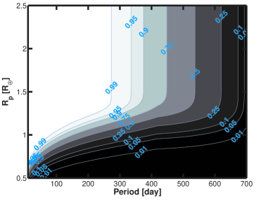
As a worked example, we demonstrate the calculation of $P_{\rm comp}$ for the host to Kepler-22b (Borucki et al., 2012). This target with Kepler Input Catalog (KIC) identifier 10593626 has stellar parameters ${R_{\star}}$=0.98 ${R_{\odot}}$, ${T_{\rm eff}}$=5640 K, $\log{\rm g}$=4.44 as compiled by the Q1-Q16 stellar catalog of Huber et al. (2014). In order to generate $P_{\rm comp}$ over the two-dimensional space of $R_{\rm p}$ and $P_{\rm orb}$ shown in Figure 1, we employ the following input values: $f_{\rm duty}=0.879$, $T_{\rm obs}=1426.7$ days, $e=0$, ${\rm MES_{\rm thresh}}=7.1$, and the 14 robCDPP noise estimates, $\sigma_{\rm cdpp,14}=[36.2,33.2,31.0,29.4,28.0,26.1,25.4,\allowbreak 24.2,23.1,22.4,21.9,21.8,21.7,21.5]$ ppm. The quantities necessary to generate $P_{\rm comp}$ for all Kepler targets searched for planets in the Q1-Q16 pipeline run are available as part of the Q1-Q16 Kepler stellar table hosted by the NASA Exoplanet Archive.

Figure 1.— Fractional completeness model for the host to Kepler-22b (KIC: 10593626) in the Q1-Q16 pipeline run using the analytic model described in Section II.

Figure 2.— Absolute difference for pipeline completeness between the analytic model described in Section II and a more accurate numerical pipeline completeness model that employs the full CDPP time series and numerical window function for the KIC target 10593626.

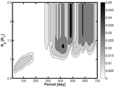
In order to investigate potential biases in the analytic pipeline completeness model, we show the absolute difference between the analytic model presented in this study and a higher fidelity completeness model that is available for future pipeline runs in Figure 2. The higher fidelity completeness model replaces two components of the completeness model described in Section II. First, the analytic window function approximation is replaced by a full numerical window function calculated during TPS to take into account data gaps and data deweighting consistent with the planet search. Second, the simplified MES estimate of Section II.1 that employs the robCDPP values is replaced by the “1-$\sigma$ depth function” (1SDF). For the 1SDF, TPS quantifies the transit signal depth that yields a MES=1 as a function of $P_{\rm orb}$ for all 14 transit durations searched taking into account the full details of the full CDPP time series and deweighted data.

Differences between the completeness estimates are largest ($\sim 0.06$) towards longer periods ($P_{\rm orb}$$\geq$ 300 days). The occurrence rate is $\propto P_{\rm comp}^{-1}$ (Youdin, 2011), thus errors in the pipeline completeness can propagate directly to occurrence rates. Future study is needed in order to characterize the net impact of the higher fidelity completeness model on occurrence rates for a full sample of Kepler targets.

Although this initial test affirms the efficacy of the analytic completeness model for this well behaved Kepler target, this comparison does not fully test all its simplifying assumptions. The above test does not check the accuracy of our assumption of a simple dependence of the pipeline completeness on MES alone and the adopted $\Delta$ to $k$ conversion. Due to a single injection per target, Christiansen et al. (2015) cannot rule out the possibility that the pipeline completeness may depend on additional parameters beyond MES and contain a strong star-by-star dependence. Results for small samples or individual targets may systematically differ from the average pipeline completeness results of Christiansen et al. (2015). However, Christiansen et al. (2015) have characterized the average pipeline completeness as a function of MES when averaged over a large sample of targets as is the case in this study. Future studies will focus on characterizing the star-by-star dependence of pipeline completeness by comparing the simplified completeness model outlined in this study to the higher fidelity completeness model using the full numerical window function and 1$\sigma$ depth function for larger samples of targets. In addition, we are implementing support for $\sim 10^{4}$ transit injections on a single target employing the NASA Ames Pleiades super computing facility (Seader et al., 2014).

An additional shortcoming of any pipeline completeness model is the inescapable dependence on the assumed stellar parameters, eccentricity, and stellar binarity. Stellar parameters and eccentricity are employed in defining $\tau_{\rm dur}$ which sets the time scale relevant for the integrated noise level, and stellar binarity can result in third light contamination that impacts the assumed planet radius. In this study, we treat the pipeline completeness as having no uncertainty due to the incomplete understanding of the stellar parameters, eccentricity, and stellar binarity. However, we do explore sensitivity in the derived planet occurrence rates to alternative assumptions for the stellar parameters and non-zero eccentricities in Section VI.2.

Although it is a distinct process separate from the pipeline generation of TCEs, the vetting classification process of TCEs into planet candidates and false positives also shapes the overall completeness of the planet candidate sample, and the vetting relied upon on a manual classification (i.e., human inspection) procedure (Mullally et al., 2015). The TCE vetting process has an unquantified false negative rate of incorrectly classifying valid planet candidates as false positives and unconscious human biases and/or errors. For this study, we assume the vetting process is 100% complete, unbiased, and correct. However, we do investigate the sensitivity of our results on this assumption in Section VI.2.4 by varying the planet candidate sample.

The analytic pipeline completeness model and input data presented in this study are only relevant to the TCE population generated by the Q1-Q16 pipeline run (Tenenbaum et al., 2014) using the SOC 9.1 software release. The next TCE release (Seader et al., 2015) used the SOC 9.2 software, which introduced changes to the data analysis and planet search algorithm that influences the pipeline sensitivity. In SOC 9.2, TPS implemented a bootstrap noise characterization algorithm during the search in order to recalibrate the detection threshold (Seader et al., 2015). The bootstrap noise characterization test allows the effective MES threshold to be a function of $P_{\rm orb}$ as opposed to being independent of $P_{\rm orb}$ in the SOC 9.1 software release. In addition, the box-car signal template matched to the data in TPS was replaced by an average limb-darkened signal template to yield a better signal match. However, changing the match template influences the noise statistics (such as robCDPP) and the $\Delta$ to $k$ conversion. Finally, the relation between pipeline completeness and MES is being analyzed through Monte-Carlo transit injection using the updated software release.

III. Stellar Properties

Precise and accurate planet occurrence rates depend on precise and accurate stellar properties. Stellar properties influence three areas relevant to planet occurrence rates: the measured planet radii, the estimated transit duration, and geometric transit probability. In this study, we adopt stellar parameters from the Q1-Q16 KIC revision of Huber et al. (2014). Huber et al. (2014) update Kepler target stellar parameters by adopting literature values and additional observations (asteroseismology, spectroscopy, and photometry) that have become available since the original KIC observations (Brown et al., 2011). With an improved observational database, Huber et al. (2014) derive stellar parameters by fitting the observations to isochrones from the Dartmouth Stellar Evolution Database (Dotter et al., 2008) using a $\chi^{2}$ minimization.

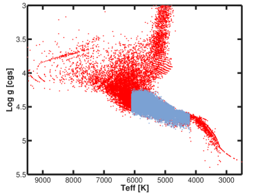
For this study we focus on planet occurrence for the G and K dwarf sample observed by Kepler. Previous occurrence rate calculations indicate significant variations in the planet population as a function of stellar ${T_{\rm eff}}$ for the Kepler sample (Howard et al., 2012; Mulders et al., 2015; Burke et al., 2015). In order to simplify the planet occurrence model by avoiding the dependence on stellar ${T_{\rm eff}}$, we focus on the GK dwarfs rather than the full FGKM dwarf sample. Burke et al. (2015) find that the planet occurrence rates agree when the G and K dwarf Kepler targets are analyzed separately in an $R_{\rm p}$ and $P_{\rm orb}$ parameter space similar to this study. We select G and K dwarfs by making the following cuts on the stellar parameter catalog of Huber et al. (2014): 4200$\leq$${T_{\rm eff}}$$\leq$6100 K and ${R_{\star}}$$\leq$ 1.15 ${R_{\odot}}$. In addition, we focus on the Kepler targets with nearly continuous coverage over the entire Q1-Q16 data span of the mission. We select targets with an observation data spanning $T_{\rm obs}>$ 2 yr, duty cycle $f_{\rm duty}>$ 0.6, and a robCDPP$\leq$ 1000 ppm at the 7.5 hr transit duration. The lower limit on $f_{\rm duty}$ ensures the inclusion of the targets that are impacted by the CCD electronics loss in Q4 of the Kepler mission (Batalha et al., 2013). The above cuts result in 91,567 targets in our sample. Figure 3 shows ${T_{\rm eff}}$ and $\log{\rm g}$ for the full catalog of Huber et al. (2014) (red points) along with the Kepler targets selected using the above criteria (gray points). Table 1 provides the Kepler identification number and a binary flag to indicate that the target belongs to the baseline stellar sample selected by the above criteria. Adopting ${T_{\rm eff}}$=5200 K as the dividing line separating the G and K dwarfs, 80% of our stellar sample belong to the G dwarf category.

Figure 3.— Stellar ${T_{\rm eff}}$ as a function of $\log{\rm g}$ for the observed Kepler targets from the Q1-Q16 stellar catalog of Huber et al. (2014) (red points), and the GK dwarf targets selected for this study (gray points). For efficient plotting only a randomly selected subsample of the full catalog is shown.

Figure 4.— Distribution of the robCDPP at the 7.5 hr time scale as a function of $K_{\rm p}$ for the G and K dwarfs analyzed in this study. Mean properties of the target stars as a function of $K_{\rm p}$ are provided in Table 2.

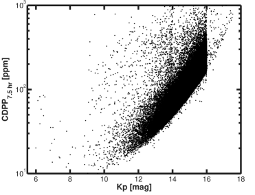
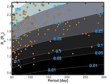
In Figure 4 we present the noise distribution of the selected GK dwarfs as a function of $K_{\rm p}$. Gilliland et al. (2011) and Christiansen et al. (2012) discuss the instrumental and astrophysical sources of noise in the Kepler data. We also provide mean properties of the GK dwarfs as a function of $K_{\rm p}$ in Table 2. In magnitude wide bins, Table 2 provides the bin centers, number of targets, mean stellar properties (${R_{\star}}$, $\log{\rm g}$, and ${T_{\rm eff}}$), and the 7.5 hr robCDPP for the 10^th, 50^th, and 90^th percentiles in each bin. Using the pipeline completeness model of Section II, we show in Figure 5 the average pipeline completeness for the GK dwarf sample in terms of detection probability contour levels over the $P_{\rm orb}$ and $R_{\rm p}$ parameter space examined in this study. The figure does not include the effects of the geometric probability to transit. We discuss our choice of $P_{\rm orb}$ and $R_{\rm p}$ space examined for this study in Section IV.

Figure 5.— Pipeline completeness model, $P_{\rm comp}$, averaged over the GK dwarf sample is shown by the contour levels over the $P_{\rm orb}$ and $R_{\rm p}$ parameter space. The Q1-Q16 Kepler planet candidate sample of Mullally et al. (2015) found around the GK dwarf sample is also shown (orange points).

Table 1Kepler GK Dwarf Target Samples

KIC ID	Baseline Sample	Original KIC Sample
757450	1	1
891901	0	1
891916	1	1
892718	1	1
892772	1	1
892832	1	1
892834	1	1
892882	1	1
892911	1	1
892946	0	1

Note. — This table is available in its entirety in a machine-readable form in the online journal. A portion is shown here for guidance regarding its form and content.

Table 2Kepler Target Summary

$K_{\rm p}$	N	$\langle$${R_{\star}}$$\rangle$	$\langle$$\log{\rm g}$$\rangle$	$\langle$${T_{\rm eff}}$$\rangle$	robCDPP7.5hr	robCDPP7.5hr	robCDPP7.5hr
$[$mag$]$		$[$${R_{\odot}}$$]$	$[$cgs$]$	$[$K$]$	10th% $[$ppm$]$	50th% $[$ppm$]$	90th% $[$ppm$]$
8	9	0.93	4.48	5658	9.3	13.1	27.4
9	36	0.90	4.48	5543	12.5	22.6	169.9
10	117	0.93	4.46	5640	13.1	23.9	169.8
11	364	0.91	4.47	5608	17.5	26.8	142.5
12	1312	0.89	4.48	5613	22.6	32.1	67.6
13	4964	0.90	4.48	5643	32.8	44.9	78.2
14	16011	0.88	4.50	5625	51.3	70.9	106.8
15	41649	0.86	4.52	5563	88.2	123.9	180.8
16	27027	0.81	4.56	5413	147.8	193.4	271.4
17	58	0.82	4.54	5201	328.0	456.0	788.9

IV. Planet Properties

We measure the planet occurrence rate using the Q1-Q16 pipeline run (Tenenbaum et al., 2014) and the resulting Kepler planet candidate sample from Mullally et al. (2015). We choose to limit our analysis to 50$\leq$$P_{\rm orb}$$\leq$300 days and rocky to mini-Neptune planets with 0.75$\leq$$R_{\rm p}$$\leq$2.5 ${R_{\oplus}}$. The $P_{\rm orb}$ range under investigation has several advantages. Mullally et al. (2015) classified the new and pre-existing KOIs into planet candidate and false positives for the $P_{\rm orb}$$>$50 days regime. Thus, the selected period range represents a uniform classification of planet candidates following the procedures of Mullally et al. (2015). The cumulative KOI catalog for $P_{\rm orb}$$<$50 days currently consists of classifications from Batalha et al. (2013), Burke et al. (2014), Rowe et al. (2015), and Mullally et al. (2015). Toward shorter and longer $P_{\rm orb}$, the population of instrumental false alarm detections increases rapidly (see bottom panel of Figure 4 in Tenenbaum et al., 2014). The vetting process employed by Mullally et al. (2015) effectively removes much of the instrumental false alarm contamination, but the remaining contamination is potentially higher outside this $P_{\rm orb}$ range.

For a majority of Kepler targets, $P_{\rm orb}$$\sim$300 days is roughly the transition between planet candidates having at least 4-5 transit events contributing to the detection and planet candidates having the minimum three transit events contributing to the detection (see Figure 9 of Burke & McCullough, 2014). The three transit event ($P_{\rm orb}$$\gtrsim$300 days) low MES planet candidates are the most challenging candidates to vet properly (Mullally et al., 2015) and further work is needed to understand the false alarm rate of this population. Thus, we exclude them from planet occurrence rate calculations for the time being. Third, approximating the behavior of the full CDPP time series by the summary robCDPP statistics for the pipeline completeness model can be inaccurate at long periods when there is an increased chance that the few transit events available can occur during outliers of the CDPP noise distribution.

The astrophysical false positive contamination rates have observationally (Santerne et al., 2012; Désert et al., 2015) and theoretically (Morton & Johnson, 2011; Fressin et al., 2013) been shown to increase towards shorter $P_{\rm orb}$. Also for shorter periods, $P_{\rm orb}$$<$3 days, the harmonic removal filter in the pipeline increasingly removes transiting planet signals (Christiansen et al., 2013, 2015). The detection efficiency reported in Christiansen et al. (2015) is calculated for $P_{\rm orb}$$>$10 days. Thus, the detection efficiency does not take into account the impact of the harmonic removal filter.

In order to select the Kepler planet candidate sample for analysis, we must limit the KOI planet candidates to ones recovered in the Q1-Q16 pipeline run. The analysis of Mullally et al. (2015) uniformly vetted the pre-existing KOIs and new KOIs that made a Threshold Crossing Event (TCE) corresponding to the KOI ephemeris for $P_{\rm orb}$$\geq$50 days. To supplement the list of planet candidates, we make special exceptions for systems with strong transit timing variations (TTV). The pipeline only searches for transits with a uniform ephemeris and targets with high SNR and strong TTVs can result in multiple TCEs at the incorrect period, but corresponding to one to a few of the high SNR transit events. If it is clear that the TCE corresponds to one or a few of the single events of a TTV system, but formally the TCE ephemeris does not match the KOI ephemeris, then that TTV KOI planet candidate is accepted as recovered by the pipeline and included in our analysis. We provide the KOI planet candidates deemed as recovered by the Q1-Q16 pipeline run in Table 3. The recovered KOIs within the 50$\leq$$P_{\rm orb}$$\leq$300 days limits for the baseline occurrence rate calculation are indicated by a binary flag in Table 3.

In addition, we provide KOI planet candidates recovered in the Q1-Q16 pipeline run in the 10$\leq$$P_{\rm orb}$$\leq$50 day range in order to support analysis of the Kepler planet candidate sample outside the parameter space of this study. The 10$\leq$$P_{\rm orb}$$\leq$50 day range has not been uniformly vetted, so for KOI recovery designations in this parameter space we start with the cumulative KOI table combining results from all the Kepler planet catalogs (Borucki et al., 2011a, b; Batalha et al., 2013; Burke et al., 2014; Rowe et al., 2015; Mullally et al., 2015). We employ an ephemeris matching routine (Mullally et al., 2015) to judge whether a Threshold Crossing Event (TCE) detection from the pipeline run (Tenenbaum et al., 2014) matches the ephemeris for the KOIs. KOIs with a match statistic satisfying that the KOI ephemeris overlaps with $\geq 90$% of the TCE’s transit events are automatically accepted as recovered. The KOI ephemeris from a previous catalog may not be accurate enough to guarantee 100% of the transit overlapping, and the 90% matching level is sufficient to automatically adopt the TCE as corresponding to the KOI without manual inspection. Also, special exception was made for systems with strong TTVs as discussed above. Table 3 lists the KOIs from the cumulative KOI list that are designated as being recovered in the Q1-Q16 pipeline run for $P_{\rm orb}$$>$10 days.

Table 3Q1-Q16 Planet Candidate Samples

KOI number	Baseline	Original KIC	High Reliability	Full Long Period	Trimmed Long Period
12.01	0	0	0	0	0
41.01	0	0	0	0	0
41.03	0	0	0	0	0
42.01	0	0	0	0	0
51.01	0	0	0	0	0
70.01	0	0	0	0	0
70.03	0	1	0	0	0
70.05	0	0	0	0	0
72.02	0	0	0	0	0
75.01	0	0	0	0	0

Note. — This table is available in its entirety in a machine-readable form in the online journal. A portion is shown here for guidance regarding its form and content.

For the planet radii, we adopt estimates from the uniform KOI analysis in Rowe et al. (2015) and Mullally et al. (2015). The technique is described fully in Rowe et al. (2014). Briefly, the flux time series data are detrended with a moving cubic polynomial fit. Data occurring during transit or near gaps are excluded from the moving polynomial fit. Assuming a circular orbit, fixed limb darkening parameters from Claret & Bloemen (2011), and stellar parameters from Huber et al. (2014), Rowe et al. (2014) use a Markov-chain Monte-Carlo methodology to estimate the best fitting parameters of a limb darkened transit model.

Overall, we find 156 planet candidates orbit stars in the GK dwarf sample within the $P_{\rm orb}$, $R_{\rm p}$ parameter space under investigation. We illustrate the planet candidate sample (orange points) in Figure 5. In our analysis described in Section V, we do not take into account the uncertainties on $R_{\rm p}$. However, we do explore the influence that systematic changes to the planet candidate sample, stellar sample, and independent model fits have on the resulting planet occurrence rates in Section VI.2.

In this study, we do not model or include the impact of astrophysical false positive contamination in our sample. Following the process outlined in Morton (2012), a preliminary astrophysical false positive analysis was completed for 108 (70%) of the baseline planet candidate sample. We find that the average and median false positive probabilities for the calculated sample are 4% and 0.6%, respectively. Twelve planet candidates in the sample have an astrophysical false positive probability $p_{\rm fpp}\geq\ 10\%$ and the highest is 60%. The astrophysical false positive contamination for the parameter space under investigation is within the statistical and systematic uncertainties and can be safely ignored for this study. However, for shorter and longer $P_{\rm orb}$, the astrophysical false positive contamination becomes increasingly important.

V. Planet Occurrence Rate Method

In order to infer the underlying planet occurrence rate from the observed distribution of Kepler planet candidates, we extend the methodology of Youdin (2011). Youdin (2011) present a parametric model for the planet distribution function (PLDF) and use likelihood maximization techniques to estimate the parameters that best describe the observed planet candidate distribution and the parameter uncertainties. We extend the method of Youdin (2011) by employing Bayesian parameter estimation theory using Markov Chain Monte-Carlo (MCMC) methods to numerically evaluate the posterior distribution of the PLDF parameters (Gregory, 2005). We were motivated to replace the intuitive and analytic minimization method of Youdin (2011) with a Bayesian MCMC parameter estimation method in order to analyze a more complicated PLDF model and enable future efforts to explore higher dimensional models including, for example, dependence on stellar parameters.

Following Youdin (2011), we employ the Poisson distribution for the likelihood. A helpful description motivating the Poisson likelihood is given in Section 5.3.2 of Loredo (1992), and the Poisson likelihood is commonly used in order to interpret astronomical detections with a varying survey sensitivity (Tabachnik & Tremaine, 2002; Allen, 2007; Cumming et al., 2008; Kraus & Hillenbrand, 2012; Foreman-Mackey et al., 2014; Nielsen et al., 2014). Also, the point process statistics literature (Daley & Vere-Jones, 1988; Baddeley, 2007) rigorously shows that the Poisson likelihood is appropriate for analyses of spatial point data. For this application, the observed planet candidate distribution is treated as an inhomogeneous Poisson process where the PLDF describes the dependence of the Poisson process intensity on $P_{\rm orb}$ and $R_{\rm p}$.

Independent of the choice of likelihood, one is free to choose any parametric form for the PLDF model. Previous work has indicated that a power law form of the PLDF describes the Kepler observations (Youdin, 2011; Howard et al., 2012; Dong & Zhu, 2013) over portions of the $R_{\rm p}$ and $P_{\rm orb}$ parameter space. For this study, we adopt a PLDF dependent upon $P_{\rm orb}$ and $R_{\rm p}$ parameterized as a power law in $P_{\rm orb}$ and a broken power law in $R_{\rm p}$ over a specified domain $P_{\rm min}\leq P_{\rm orb}\leq P_{\rm max}$ and $R_{\rm min}\leq R_{\rm p}\leq R_{\rm max}$:

$$\frac{{\rm d}^{2}f}{{\rm d}P_{\rm orb}{\rm d}R_{\rm p}}=F_{0}\,C_{\rm n}\,g(P_{\rm orb},R_{\rm p})\\ =\left\{\begin{array}[]{lr}F_{0}\,C_{\rm n}\left(\frac{P_{\rm orb}}{P_{\rm o}}\right)^{\beta}\left(\frac{R_{\rm p}}{R_{\rm o}}\right)^{\alpha_{1}}&{\rm if}\,R_{\rm p}<R_{\rm brk}\\ F_{0}\,C_{\rm n}\left(\frac{P_{\rm orb}}{P_{\rm o}}\right)^{\beta}\left(\frac{R_{\rm p}}{R_{\rm o}}\right)^{\alpha_{2}}\left(\frac{R_{\rm brk}}{R_{\rm o}}\right)^{\alpha_{1}-\alpha_{2}}&{\rm if}\,R_{\rm p}\geq R_{\rm brk}\end{array}\right.,$$ (7)

where $F_{0}$ is the integrated planet occurrence rate, $C_{\rm n}$ is a normalization factor, $g({\bf x})$ is the shape function, $P_{\rm o}=(P_{\rm min}+P_{\rm max})/2$ and $R_{\rm o}=(R_{\rm min}+R_{\rm max})/2$ are domain scaling factors, $R_{\rm brk}$ is the break radius transition between the two $R_{\rm p}$ power law exponents ($\alpha_{1}$ and $\alpha_{2}$), and $\beta$ is the $P_{\rm orb}$ power law exponent. The $C_{\rm n}$ is determined from the normalization requirement,

$$\int\limits_{P_{\rm min}}^{P_{\rm max}}\int\limits_{R_{\rm min}}^{R_{\rm max}}\,C_{\rm n}\,g(P_{\rm orb},R_{\rm p}){\rm d}P_{\rm orb}{\rm d}R_{\rm p}=1.$$ (8)

Overall, the PLDF has five free parameters: $F_{0}$, $\beta$, $\alpha_{1}$, $\alpha_{2}$, and $R_{\rm brk}$. Following Equation (18) of Youdin (2011), the Poisson likelihood of the data for a survey that detects $N_{\rm pl}$ planets around $N_{\star}$ survey targets is

$$L\propto\left[F_{0}^{N_{\rm pl}}\,C_{\rm n}^{N_{\rm pl}}\prod\limits_{i=1}^{N_{\rm pl}}\,g(P_{\rm orb},R_{\rm p})\right]\exp(-N_{\rm exp}),$$ (9)

where the PLDF model predicted number of detections from the survey is

$$N_{\rm exp}=F_{0}\,C_{\rm n}\,\int\limits_{P_{\rm min}}^{P_{\rm max}}\int\limits_{R_{\rm min}}^{R_{\rm max}}\,\left[\sum\limits_{j=1}^{N_{\star}}\,\eta_{j}(P_{\rm orb},R_{\rm p})\right]\,g(P_{\rm orb},R_{\rm p}){\rm d}P_{\rm orb}{\rm d}R_{\rm p},$$ (10)

and the likelihood ignores constant multiplicative factors. In Equation (10), the underlying PLDF model is modified by the per-star transit survey effectiveness, $\eta_{j}({\bf x})$, summed over $N_{\star}$ targets in the sample, where $\eta_{j}({\bf x})=P_{j,{\rm comp}}\times P_{j,{\rm tr}}$ is the per-star pipeline completeness model of Section II and $P_{j,{\rm tr}}$ is the geometric probability to transit. The transit probability factor, $P_{j,{\rm tr}}=(R_{\star}/a)/(1-e^{2})$, depends on the stellar parameters and orbital eccentricity (Burke, 2008).

The separable form between $R_{\rm p}$ and $P_{\rm orb}$ of the PLDF adopted in this study, is overly restrictive if applied to a larger range of $R_{\rm p}$. Previous studies have identified a dependence of the $P_{\rm orb}$ exponent, $\beta$, on planet radius (Dong & Zhu, 2013; Foreman-Mackey et al., 2014), with an apparent transition in the $P_{\rm orb}$ dependence around $R_{\rm p}$$\sim$4${R_{\oplus}}$. For the 0.75$\leq$$R_{\rm p}$$\leq$2.5 ${R_{\oplus}}$ analysis region of this study we do not find evidence for a more complicated dependence between $R_{\rm p}$ and $P_{\rm orb}$ being necessary based upon residuals between the observed and model fitted planet counts. Also of note in Equation (10), is that the summation of $\eta_{j}$ over the stellar sample is independent of the PLDF parameters. Thus, the summation can be computed once for the analysis and the planet occurrence depends upon the integrated/average transit survey effectiveness alone rather than explicitly depending upon the per-star survey effectiveness.

We complete the Bayesian posterior calculation by specifying uniform priors for all parameters except for $F_{0}$ which has a prior that is uniform in the logarithm. The adopted MCMC implementation for this analysis is based upon the description in Gregory (2005) that employs a Metropolis-Hastings algorithm with an automated iterative proposal step-size determination and has been applied to transit model light curve analysis (Burke et al., 2007), transit timing analysis (Burke et al., 2010), and radial velocity analysis (Charbonneau et al., 2009; Ballard et al., 2011). For this study, we do not incorporate uncertainty in $R_{\rm p}$and ignore contributions to the planet candidate sample due to astrophysical and instrumental false positives (see Youdin, 2011; Mullally et al., 2015, for a more in-depth discussion). In the case of multiple planet systems, adopting the Poisson likelihood treats multiple planets in a system as independent, and thus this method can not capture any structure and correlations between planet’s in a single system, but captures the average behavior over a large sample of stars. However, we do constrain the sensitivity of our results to these potential complications in Section VI.2.

VI. Results

In this section, we provide planet occurrence rate determinations based upon the Q1-Q16 Kepler planet candidate sample of Mullally et al. (2015) (see Section IV and Table 3). We focus on the GK dwarf targets observed by Kepler using stellar parameters from the catalog of Huber et al. (2014) (see Section III and Table 1). We describe our analytic pipeline completeness model in Section II that employs the pipeline detection efficiency as calibrated by the Monte-Carlo transit injection and recovery provided by Christiansen et al. (2015). The planet occurrence rate is derived through a parameterized model for the PLDF, where the parameters and their uncertainties are determined within a Bayesian parameter estimation problem with the posterior estimated through MCMC techniques (see Section V). The above set of inputs represents our current best/baseline model for planet occurrence rates, and we describe the results in Section VI.1. We then perform a sensitivity analysis in Section VI.2 in order to explore the systematic uncertainty in the planet occurrence rates due to imprecise knowledge of the baseline inputs.

VI.1. Baseline Results

For the baseline result, we fit the PLDF over the parameter space of 0.75$<$$R_{\rm p}$$<$2.5 ${R_{\oplus}}$ and 50$<$$P_{\rm orb}$$<300$ days. We tabulate 10,000 subsamples from the full MCMC posterior samples for all the parameters along with the resulting likelihood and prior values in Table 4. The overall occurrence rate for this parameter space $F_{0}=0.77\pm 0.12$ planets per star. Relying on the statistical uncertainty alone, the 3-$\sigma$ upper limit $F_{0,3\sigma\,\rm U.L.}=1.3$ implies that we cannot currently rule-out a scenario that when averaged over large samples of GK dwarfs there exists more planets in the analyzed parameter space than stellar hosts. The 3-$\sigma$ lower limit $F_{0,3\sigma\,\rm L.L}=0.49$ implies that for large samples of GK dwarfs there exists on average at least one planet in the analyzed parameter space for every two stellar hosts.

Table 4PLDF Model Parameter Posterior Samples

$\alpha_{1}$	$\alpha_{2}$	$R_{\rm brk}$	$\beta$	$F_{0}$	Ln(Likelihood)	Ln(Prior)
-1.80587	9.60189	2.42398	-0.53218	1.04356	-1154.1220	-11.3374
-0.91336	-7.31895	2.20004	-0.68832	0.74751	-1152.1463	-11.3374
-2.55130	-1.50156	1.71089	-0.78946	1.04314	-1156.0940	-11.3374
16.62721	-1.43560	0.91343	-0.68223	0.69378	-1151.8822	-11.3374
6.77569	-1.25637	0.87505	-0.61621	0.67331	-1153.4823	-11.3374
-1.34402	-7.41157	2.37924	-0.45503	0.93427	-1155.0970	-11.3374
-1.90010	-3.45914	2.01354	-0.91872	0.97944	-1155.2124	-11.3374
6.59736	-1.64782	1.00841	-0.55609	0.71677	-1152.5281	-11.3374
-1.96796	-3.36621	2.29527	-0.34320	1.02223	-1155.7010	-11.3374
16.05061	-2.14134	0.94454	-0.76077	0.83308	-1152.5983	-11.3374

Note. — This table is available in its entirety in a machine-readable form in the online journal. A portion is shown here for guidance regarding its form and content.

Figure 6 shows how well the parametric PLDF model predicts the observed, uncorrected Kepler planet candidate counts summed over 50$<$$P_{\rm orb}$$<$300 days in d$R_{\rm p}$=0.25 ${R_{\oplus}}$ sized bins (points with uncertainties). Evaluating the PLDF at the parameters that maximize the likelihood fit to the data, we show the model predicted counts ($N_{\rm exp}$ of Equation (10) where the limits of integration are 50$<$$P_{\rm orb}$$<$300 days and d$R_{\rm p}$=0.25 ${R_{\oplus}}$) as the white dashed line. In addition, we show the median (solid blue line), 1-$\sigma$ (orange region), and 3-$\sigma$ (blue region) model predicted counts by evaluating $N_{\rm exp}$ using 10,000 random samples from the posterior PLDF parameter estimates from the MCMC chain. Figure 7 shows the equivalent information, but along the $P_{\rm orb}$ dimension after marginalizing over 0.75$<$$R_{\rm p}$$<$2.5 ${R_{\oplus}}$ and d$P_{\rm orb}$=31.25 days. The bin sizes for the abcissae in Figures 6 and 7 are chosen in order to balance segmenting the parameter space range into a high number of evenly sized bins and maintaining at least three detections in each bin.

Figure 6.— Comparison between the predicted planet sample from the planet occurrence rate model and the observed Kepler planet candidate sample. The observed, marginalized over 50$<$$P_{\rm orb}$$<$300 days, histogram of Kepler planet candidate counts as a function of $R_{\rm p}$ (points) can be compared to the maximum likelihood model for the predicted counts (white dash line). Also shown is the posterior distributions of the model predicted counts for the median (blue solid line), 1-$\sigma$ region (orange region), and 3-$\sigma$ region (blue region) marginalized over $P_{\rm orb}$ and in bins of d$R_{\rm p}$=0.25 ${R_{\oplus}}$.

Figure 7.— Same as Figure 6, but marginalized over 0.75$<$$R_{\rm p}$$<$2.5 ${R_{\oplus}}$and bins of d$P_{\rm orb}$=31.25 days.

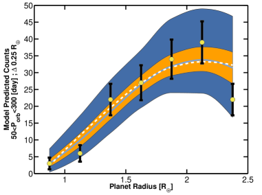
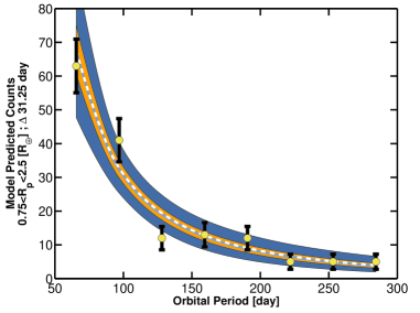
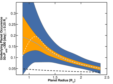
Figure 8 quantifies the underlying PLDF free of the deleterious effects of the Kepler pipeline completeness and geometric transit probability. The white dashed line, representing the PLDF for parameters that maximize the likelihood of the data, rises toward small planets with $\alpha_{2}=-1.8$ and has a break near the edge of the parameter space. Given the low numbers of observed planet candidates in the smallest planet bins, the full posterior allowed behavior (1-$\sigma$ orange region ; 3-$\sigma$ blue region) cannot distinguish between a rising or falling PLDF for $R_{\rm p}$$\lesssim 1.5$ ${R_{\oplus}}$. Figure 9 shows the equivalent information, but along the $P_{\rm orb}$ dimension after marginalizing over 0.75$<$$R_{\rm p}$$<$2.5 ${R_{\oplus}}$ and d$P_{\rm orb}$=31.25 days.

Figure 8.— Shows the underlying planet occurrence rate model. Marginalized over 50$<$$P_{\rm orb}$$<$300 days and bins of d$R_{\rm p}$=0.25 ${R_{\oplus}}$ planet occurrence rates for the model parameters that maximize the likelihood (white dash line). Posterior distribution for the underlying planet occurrence rate for the median (blue solid line), 1-$\sigma$ region (orange region), and 3-$\sigma$ region (blue region). An approximate PLDF based upon results from Petigura et al. (2013b) for comparison (dash dot line).

Figure 9.— Same as Figure 8, but marginalized over 0.75$<$$R_{\rm p}$$<$2.5 ${R_{\oplus}}$ and bins of d$P_{\rm orb}$=31.25 days.

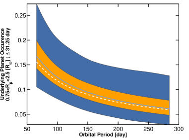
Formally, in our baseline analysis of the GK dwarf sample, the double power law in the $R_{\rm p}$ model is unwarranted relative to a single power law according to the Bayesian information criterion (BIC) methodology for model comparison. However, we choose to provide the final results in terms of the double power law model for the following reasons: (a) The additional flexibility of the double power law model provides a better fit to the smallest $R_{\rm p}$ parameter space of most interest, whereas the single power law model systematically overestimates (by $\sim$0.5 $\sigma$ in a comparable data/model comparison to that shown in Figure 6) the occurrence rates in the smallest $R_{\rm p}$ bins. (b) The more complicated model ensures the ability to adapt to variations in the PLDF in the sensitivity analysis of Section VI.2. (c) Previous work on Kepler planet occurrence rates indicated a break in the planet population for 2.0$\lesssim$$R_{\rm p}$$\lesssim$2.8 ${R_{\oplus}}$ (Fressin et al., 2013; Petigura et al., 2013a, b; Silburt et al., 2015). (d) Finally, extending this work to a larger parameter space and for alternative target selection samples, such as the Kepler M dwarf sample where a sharp break at $R_{\rm p}$$\sim$2.5 ${R_{\oplus}}$ is observed (Dressing & Charbonneau, 2013; Burke et al., 2015), the double power law in $R_{\rm p}$ is strongly (BIC$>10$) warranted.

Symptomatic of the weak evidence for a broken power law model over the 0.75$\leq$$R_{\rm p}$$\leq$2.5 ${R_{\oplus}}$ range, $R_{\rm brk}$ is not constrained within the prior $R_{\rm p}$ limits of the parameter space. When $R_{\rm brk}$ is near the lower and upper $R_{\rm p}$ limits, $\alpha_{1}$ and $\alpha_{2}$ also become poorly constrained, respectively. To provide a more meaningful constraint on the average power law behavior for $R_{\rm p}$ in the double power law PLDF model, we introduce $\alpha_{\rm avg}$, which we set to $\alpha_{\rm avg}=\alpha_{1}$ if $R_{\rm brk}\geq R_{\rm mid}$ and $\alpha_{\rm avg}=\alpha_{2}$ otherwise, where $R_{\rm mid}$ is the midpoint between the upper and lower limits of $R_{\rm p}$. We find $\alpha_{\rm avg}=-1.54\pm 0.5$ and $\beta=-0.68\pm 0.17$ for our baseline result. We use $\alpha_{\rm avg}$ as a summary statistic for the model parameters only to enable a simpler comparison of our results to independent analyses of planet occurrence rates and to approximate the behavior for the power law $R_{\rm p}$ dependence if we had used the simpler single power law model. The results for a single power law model in both $R_{\rm p}$ and $P_{\rm orb}$ are equivalent to the results for the double power law model ($F_{0}=0.83\pm 0.13$, $\alpha=-1.56\pm 0.3$, and $\beta=-0.68\pm 0.17$).

In Table 5, we provide the parameters of the PLDF that maximizes the likelihood for the data in our baseline analysis as well as the median and percentile posterior values for $F_{0}$, $\beta$, and $\alpha_{\rm avg}$. Additional statistics for the full five parameter PLDF can be estimated from the 10,000 posterior MCMC samples in Table 4.

Table 5PLDF Model Parameter Summary

	$F_{0}$	$\alpha_{1}$	$\alpha_{2}$	$R_{\rm brk}$	$\alpha_{\rm avg}$	$\beta$
Likelihood Max	0.73	19.68	-1.78	0.94	…	-0.65
0.13%	0.48	…	…	…	-3.09	-1.20
15.9%	0.66	…	…	…	-1.97	-0.85
50.0%	0.77	…	…	…	-1.54	-0.68
84.1%	0.92	…	…	…	-1.04	-0.35
99.9%	1.32	…	…	…	0.53	-0.19
Lower Limit	0.28	…	…	…	-3.25	-1.4
Upper Limit	1.92	…	…	…	0.53	-0.10

VI.2. Sensitivity Analysis

Planet occurrence rate calculations are only as accurate as the inputs. The baseline results of Section VI represent our current best set of data that are uniformly applicable to the Kepler observations and planet search results. The resulting posterior distribution for the PLDF parameters in the above analysis only represent their statistical precision and do not capture potential sources of systematic uncertainties present in the inputs. To explore the level of systematic errors present in the current results, we repeat the baseline analysis, but for several scenarios in which we change a single input. The following sections describe results of these sensitivity tests.

VI.2.1 Pipeline Completeness Systematics

The pipeline detection efficiency we employ for the baseline analysis is calibrated with transit injection and recovery tests (Christiansen et al., 2015), but it represents the pipeline response averaged over a wider range of Kepler targets than the limited GK dwarf sample of this study. In addition, Christiansen et al. (2015) analyzed a shorter (four Kepler quarter) subset of the entire Q1-Q16 data. It is expected that the pipeline completeness primarily depends upon the MES and number of transits, thus the results from the shorter four quarter analysis are applicable to the sixteen quarter run. However, star-by-star deviations are expected, and until we perform larger injection studies it is prudent to investigate the sensitivity of the occurrence rates to this potential source of uncertainty. We consider an optimistic and pessimistic detection efficiency relative to the baseline result. For the optimistic detection efficiency, we assume the ideal theoretical expected performance of TPS given by Equation (4). For the pessimistic detection efficiency we assume the result from Fressin et al. (2013), where they find a linear detection efficiency over the range 6$<$MES$<$16 provides the best match to the SNR distribution of the Q1-Q6 Kepler planet candidate sample (Batalha et al., 2013). The detection efficiency of the Q1-Q6 Kepler pipeline was never measured directly using Monte-Carlo transit recovery tests. Thus, we cannot determine the accuracy of the Fressin et al. (2013) detection efficiency relative to the Q1-Q6 Kepler pipeline run. However, having measured the detection efficiency for the Q1-Q16 pipeline run (Christiansen et al., 2015), the Fressin et al. (2013) detection efficiency is overly pessimistic for the pipeline completeness of the Q1-Q16 pipeline run.

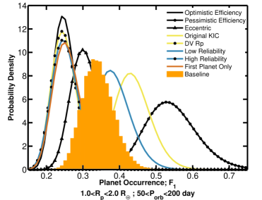
Overall, an overly optimistic detection efficiency reduces the planet occurrence rate and a pessimistic detection efficiency increases the planet occurrence rates. We show in Figure 10 the posterior integrated planet occurrence rate for the baseline result (orange histogram) compared to the case of an optimistic (black line) and the pessimistic (black with circles line) detection efficiency alternatives. For this comparison we narrow the parameter space of integration (1.0$<$$R_{\rm p}$$<$2.0 ${R_{\oplus}}$ and 50$<$$P_{\rm orb}$$<$200 days) in order to limit the comparison to a region of parameter space with better statistics and to facilitate comparison with Kepler occurrence rates from previous studies. We symbolize this narrower parameter space planet occurrence rate as $F_{1}$. For clarity of display in Figure 10, the optimistic and pessimistic occurrence rate posteriors are shown by a log-normal fit to the posterior rather than the full posterior detail in a histogram format. The pessimistic detection efficiency has a $>$3-$\sigma$ larger occurrence rate than the baseline result and the optimistic detection efficiency is 2.5-$\sigma$ lower than the baseline result. This initial test demonstrates that systematic effects can be larger than the random uncertainties.

Figure 10.— Posterior distribution for the integrated planet occurrence rate over the 1.0$<$$R_{\rm p}$$<$2.0 ${R_{\oplus}}$ and 50$<$$P_{\rm orb}$$<$200 days parameter space, $F_{1}$. Changes from the baseline inputs (filled orange histogram) systematically impact the derived occurrence rate beyond the statistical uncertainty. We discuss in Section VI.2 alternative inputs: optimistic detection efficiency (black line), pessimistic detection efficiency (black with circles line), assuming e=0.4 for all orbits (black with triangles line), original KIC stellar parameters (yellow line), alternative DV $R_{\rm p}$ (yellow with circles line), low reliability planet candidate sample (blue line), high reliability planet candidate sample (blue with circles line), and assuming a single planet search (red line).

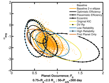
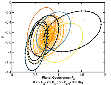
The alternative inputs also influence the other ‘shape’ parameters of the PLDF. We show samples from the posterior distribution of $\alpha_{\rm avg}$ (Figure 11) and $\beta$ (Figure 12) as a function of $F_{0}$ for the baseline (orange points) occurrence rate parameter estimates. As an approximation to the joint 2-$\sigma$ posterior distribution we model the posterior as a multi-normal distribution with major and minor axes along the eigenvectors determined from the posterior samples (orange ellipse). For comparison, we show the optimistic (black ellipse) and pessimistic (black with circles ellipse) detection efficiency solutions by the 2-$\sigma$ ellipse model for the shape parameters. The systematic variations of $\alpha_{\rm avg}$ and $\beta$ are correlated with $F_{0}$.

Figure 11.— Samples from the posterior distribution of $F_{0}$ as a function $\alpha_{\rm avg}$ for the baseline results (orange points) along with an approximate 2-$\sigma$ error ellipse for the baseline results (orange ellipse). Also shown are 2-$\sigma$ error ellipses for the alternative inputs with the same line types as in Figure 10.

Figure 12.— Same as Figure 11, but showing the posterior distribution of $F_{0}$ as a function $\beta$.

VI.2.2 Orbital Eccentricity

In the baseline result we have assumed circular orbits when constructing the model for pipeline completeness. However, radial velocity studies have revealed that eccentric orbits are common for $P_{\rm orb}$$>$10 days (Butler et al., 2006). A nonzero eccentricity results in higher probability to transit, but a shorter transit duration degrades the transit SNR (Burke, 2008). Burke (2008) shows that yields from a transit survey could be up to 25% higher using the observed distribution of radial velocity planets. We investigate a limiting case of assuming all planets have e=0.4. The e=0.4 case results in an 11% (1-$\sigma$) lower planet occurrence rate (black with triangles line in Figure 10). Thus, for this parameter space the systematic effect due to orbital eccentricity is comparable to the statistical errors. The impact of eccentricity on $\alpha_{\rm avg}$ and $\beta$ is also modest.

VI.2.3 Stellar Parameter Systematics

Stellar parameter estimates of Kepler targets are subject to systematic uncertainties (Brown et al., 2011; Mann et al., 2012; Muirhead et al., 2012; Pinsonneault et al., 2012; Dressing & Charbonneau, 2013; Everett et al., 2013; Gaidos & Mann, 2013) and multiplicity/blend effects (Cartier et al., 2014; Lillo-Box et al., 2014; Ciardi et al., 2015). Also, the stellar parameter catalog of Huber et al. (2014) relies upon a heterogeneous compilation of input sources and still has some limitations (see their Section 8 for a discussion). As a proxy for constraining the impact on occurrence rate studies due to stellar parameter systematics, we repeat the analysis but adopt stellar parameters from the original KIC (Brown et al., 2011). Using the original KIC is also germane since it was employed for previous work on planet occurrence rates with Kepler (Howard et al., 2012; Fressin et al., 2013).

We redo the GK dwarf target selection resulting in 102,186 targets that meet the selection criteria. There are 83,724 targets (91.4%) in common with the baseline GK dwarf sample discussed in Section III. Table 1 provides a binary flag to indicate that the Kepler target was included in the stellar sample based upon the original KIC stellar parameters. In the original KIC GK dwarf sample there are 177 planet candidates that have 122 planet candidates (78.2%) in common with the baseline planet candidate sample discussed in Section IV. Table 3 has a binary flag indicating the planet candidates selected for this original KIC stellar sample. We adjust the derived $R_{\rm p}$ of the planet candidate sample by linearly scaling $R_{\rm p}$ by the ratio in ${R_{\star}}$ between the baseline and the original KIC values.

The net impact of the alternative stellar parameters results in $\sim 2\sigma$ higher occurrence rates (yellow line in Figure 10). The change in $\alpha_{\rm avg}$ is larger than for $\beta$ (yellow ellipse in Figures 11 and 12).

VI.2.4 Planet Candidate Parameters

Planet radii are not a direct observable, and they must be derived through parameter fits to light curves with various assumptions as to the stellar parameters, limb darkening coefficients, flux time series detrending, treatment of instrumental effects, orbital eccentricity, and third light contamination to name a few (Mandel & Agol, 2002; Seager & Mallén-Ornelas, 2003; Giménez, 2006; Holman et al., 2006; Burke et al., 2007; Torres et al., 2008; Southworth, 2011; Kipping, 2014; Rowe et al., 2015; Mullally et al., 2015; Ciardi et al., 2015). In our current analysis, we treat $R_{\rm p}$ as perfectly known without uncertainty. Recent work has pointed out the non-negligible bias in deriving planet occurrence rates without taking into account the full error distribution of $R_{\rm p}$ (Morton & Swift, 2014; Foreman-Mackey et al., 2014; Silburt et al., 2015; Dressing & Charbonneau, 2015). Detailed planet parameter posterior estimates have only recently become available for a majority of the Kepler planet candidate sample (Rowe et al., 2015), thus we defer occurrence rate analysis using a full posterior distribution of planet radii for future work.

We repeat the occurrence rate calculation using the alternative $R_{\rm p}$ estimates provided by the Data Validation (DV) module of the Kepler pipeline (Wu et al., 2010). The most important differences between the DV analysis and the baseline planet parameters from Mullally et al. (2015) and Rowe et al. (2014) are the independent methods of detrending the flux time series data and DV use of $\chi^{2}$ minimization instead of a MCMC analysis. Both analyses assume the same stellar parameters, fixed limb darkening coefficients, zero eccentricity, and begin with the pre-search data conditioning time series (Stumpe et al., 2012; Smith et al., 2012). Mullally et al. (2015) find that the radii ratios, $R_{\rm p}$/${R_{\star}}$, from the MCMC analysis are $\sim$7% smaller than from the analysis in DV. The typically larger $R_{\rm p}$ from DV results in $\sim 2.2\sigma$ lower occurrence rates (yellow with circles line in Figure 10). The change in $\alpha_{\rm avg}$ is larger than for $\beta$ (yellow with circles ellipse in Figures 11 and 12).

VI.2.5 Planet Candidate Sample

Characterizing a detection by the Kepler pipeline as a bona fide member of the Kepler planet candidate sample has increasingly relied upon an automated classification procedure (McCauliff et al., 2014; Rowe et al., 2015; Mullally et al., 2015; Coughlin et al., 2015; Rowe et al., 2015). However, the accuracy, efficacy, and impact on deriving planet occurrence rates due to the automated classification and remaining manual vetting decision steps have not been fully quantified. The vetting process has its own false negative alarm rate outside of the pipeline completeness, that currently we do not account for. In addition, the decision process for both the automated and manual decision methods becomes increasingly less definitive towards low SNR (see the discussion of the current planet sample limitations in Sections 7 and 9.1 of Mullally et al., 2015). The planet candidate catalog of Mullally et al. (2015) takes an ‘innocent until proven guilty’ approach to deal with the indeterminant diagnostics in the low SNR regime. The instrumental aperture contamination and crosstalk also become increasingly difficult to identify at low SNR (Coughlin et al., 2014). We constrain the potential systematics in deriving planet occurrence rates due to uncertainty in the planet candidate sample classification process by considering two alternative planet samples.

First, we include a population of twelve ‘lower reliability’ KOIs with a false positive disposition in the 50$\leq$$P_{\rm orb}$$\leq$300 days and $R_{\rm p}$$\leq$2.5 ${R_{\oplus}}$ parameter space under investigation (see Table 6). This sample of ‘lower reliability’ KOIs were characterized as planet candidates for all the vetting procedures described in Mullally et al. (2015) except one. These KOIs are false positives because they failed to maintain an SNR$\geq 7.1$ in the independent detrending employed for the MCMC planet parameter estimates (Rowe et al., 2014). Prior to the MCMC evaluation, a trial $\chi^{2}$ minimization provides a parameter initialization. These lower reliability KOIs failed to yield SNR$\geq 7.1$ in this trial fit and were therefore demoted from a PLANET CANDIDATE to a FALSE POSITIVE disposition. Requiring an independent recovery of a potential detection is a valuable criteria for a planet candidate, but it largely impacts our lowest SNR detections and we have not fully quantified the false negative rate of this independent recovery test. In lieu of a more detailed investigation, it provides a useful limiting test case sample to constrain the potential breakdown of the vetting metrics at the lowest SNR of the planet candidate sample. Including a lower reliability KOI sample in the planet candidate list, results in $\sim 1\sigma$ higher occurrence rates (blue line in Figure 10) and modest changes in $\alpha_{\rm avg}$ and $\beta$ (blue ellipse in Figures 11 and 12).

Table 6Low Reliability KOI False Positive Sample

KOI number
4954.01
5043.01
5081.01
5102.01
5123.01
5177.01
5198.01
5210.01
5257.01
5309.01
5325.01
5405.01

Second, we cull the baseline KOI planet candidate sample to the most reliable detections by requiring KOIs to have been detected in at least one other pipeline run. Each run of the Kepler pipeline is independent and has different amounts and versions of the data. To remain in the ‘high reliability’ planet candidate sample, we require a KOI to be represented as a TCE in either the Q1-Q12 pipeline run (Tenenbaum et al., 2013; Rowe et al., 2015), the Q1-Q17 pipeline run (Seader et al., 2015), or a testing/development run using Q1-Q17 data with a near-final Kepler pipeline code version. This requirement removed 26 KOI planet candidates in the 50$\leq$$P_{\rm orb}$$\leq$300 days and $R_{\rm p}$$\leq$2.5 ${R_{\oplus}}$ parameter space under investigation. Table 3 contains a binary flag indicating the planet candidates belonging to this high reliability planet sample. Adopting a higher reliability KOI sample results in $\sim 2.2\sigma$ lower occurrence rates (blue with circles line in Figure 10). The change in $\alpha_{\rm avg}$ and $\beta$ (blue with circles ellipse in Figures 11 and 12) are consistent with preferentially removing the lower SNR KOIs which typically reside at smaller radii and longer orbital periods.

The final systematic we investigate is the impact of limiting the search to a single planet per target, effectively ignoring the multiple planet search in the Kepler pipeline. We provide this result in order to more directly compare independent analyses of the Kepler data that do not search for multiple planets (Petigura et al., 2013b). Petigura et al. (2013b) estimate that their occurrence rates would be $\sim$25% higher by including multiple planet systems in their study. We concur with their estimate by finding a 25% ($\sim 2.2\sigma$) lower occurrence rate by only including the lowest numbered KOI (typically the highest SNR) of a system (red line in Figure 10). The change in $\alpha_{\rm avg}$ is negligible and $\beta$ prefers a more gradual decrease in planet occurrence with $P_{\rm orb}$ despite the lower overall occurrence rate normalization (red ellipse in Figures 11 and 12).

VI.2.6 Systematic Error Summary

The previous sections show that individual systematic effects can reach 2$\sigma$ biases in the occurrence rates, where $\sigma$ is determined from statistical errors alone. Unfortunately, multiple systematic effects can add coherently rather than quadratically (see Section VII). To provide a more realistic uncertainty in the context of all these systematic uncertainties, we express the uncertainties on the occurrence rate parameters as an acceptable range. We adopt the lower and upper limit of the acceptable range as the 2$\sigma$ lower and upper limit for the largest systematic effect calculated in the previous sections. Based upon the results in this section, we find that the planet occurrence rate for the 1.0$<$$R_{\rm p}$$<$2.0 ${R_{\oplus}}$ and 50$<$$P_{\rm orb}$$<$200 days parameter space to have a best value from the baseline calculation of $F_{1}=0.34$ with an acceptable range of 0.19$\leq F_{1}\leq$0.7. We provide acceptable ranges for the PLDF model parameters in Table 5.

VII. Discussion

In this section, we compare our PLDF to previous work on the Kepler target sample that included analysis of the G dwarf targets using at least twelve quarters of Kepler data. We generally find higher occurrence rates, no evidence for a break at $R_{\rm p}$$\lesssim$2.5 ${R_{\oplus}}$, increasing planet occurrence rates towards $R_{\rm p}$=1.0 ${R_{\oplus}}$, slightly shallower drop-off of occurrence rates towards longer $P_{\rm orb}$, and larger uncertainty on occurrence rates driven by systematic effects.

As a primary source for comparison, we compare to the independent pipeline analysis on planet occurrence rates by Petigura et al. (2013b). We compare the integrated planet occurrence rate over the 1.0$<$$R_{\rm p}$$<$2.0 ${R_{\oplus}}$ and 50$<$$P_{\rm orb}$$<$200 days range, $F_{1}$, in Figure 13. We approximate the result from Petigura et al. (2013b) ($F_{1}$=9$\pm$3% occurrence rate) as a Gaussian (black line) with value and uncertainty as published from their Figure 2. The posterior distribution of our baseline result (orange histogram) demonstrates a significant difference from the occurrence rate of Petigura et al. (2013b). For consistency with the TERRA pipeline (which does not search for multiple planets), we show our alternative occurrence rate after keeping only the highest SNR planet candidate for a target (red line) in Figure 13. The ‘first planet only’ occurrence rate does not fully remove the difference. In our analysis we explored numerous alternative inputs (see Section VI.2). Even when assuming a wide variety of systematics, we have a difficult time reconciling our results with Petigura et al. (2013b).

Figure 13.— Comparison of the integrated posterior distribution from our baseline PLDF over the 1.0$<$$R_{\rm p}$$<$2.0 ${R_{\oplus}}$ and 50$<$$P_{\rm orb}$$<$200 days parameter space (orange filled histogram) to previous results over the same parameter space from Petigura et al. (2013b) (black curve) and Mulders et al. (2015) (blue curve). The posterior distribution from the other works are approximated as Gaussians with their central and standard deviation parameters as published. We also show our single planet search results (red line) and an extreme scenario where the four leading systematics resulting in lower occurrence rates are combined (red with circles line, see Section VII).

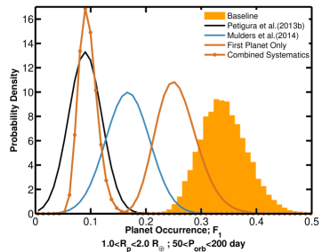
It is possible that several sources of systematics add coherently to reconcile the results. For instance, we can reproduce the occurrence rate of Petigura et al. (2013b) (black line in Figure 13) by combining together four of the systematic effects resulting in lower occurrence rates: single planet search only, alternative DV $R_{\rm p}$, highest reliability KOIs, and optimistic detection efficiency. The resulting occurrence rate (red with circles line in Figure 13) $F_{1}=0.09$ is less than our lower limit of an acceptable range $F_{1}\geq 0.19$. Further work is needed to understand the differences between our results and the results of Petigura et al. (2013b). Some possibilities including increasing the number of injection and recovery trials, characterizing the impact of the flux time series detrending on planet recovery, investigating systematic differences between the stellar parameter estimates of the planet candidate hosts and non planet candidate hosts, and better characterization of the biases that may be present when using the binned occurrence rate methodology (Morton & Swift, 2014). For instance, Foreman-Mackey et al. (2014) note a bias in the binned occurrence rate methodology is present if the completeness function is evaluated at exactly the location of the planet parameters rather than being averaged over the entire bin of analysis.

One characteristic result of Petigura et al. (2013b) is a plateau to declining occurrence rates in the mini-Neptune to terrestrial planet regime. To enable comparison of the results from our parametric PLDF model, we derive an approximate PLDF consistent with the occurrence rate from Figure 3 of Petigura et al. (2013b), marginalized over 5$<$$P_{\rm orb}$$<$100 days. We determine a PLDF with two free parameters, $g_{\rm p}=F_{\rm p}R_{\rm p}^{\alpha_{\rm p}}P_{\rm orb}^{-1}$, using the 1$\leq$$R_{\rm p}$$\leq$1.4 ${R_{\oplus}}$ and 2$\leq$$R_{\rm p}$$\leq$2.8 ${R_{\oplus}}$ bins from Figure 3 of Petigura et al. (2013b), yielding $\alpha_{\rm p}=-0.3677$ and $F_{\rm p}=0.103$. The approximating PLDF yields an occurrence rate of 14.9% for the 1.4$\leq$$R_{\rm p}$$\leq$2.0 ${R_{\oplus}}$ bin compared to the published value of 14.2$\pm$1.0% from Petigura et al. (2013b). As a further check, the approximating PLDF yields a $F_{1}$=12.5% occurrence rate compared to $F_{1}$=9$\pm$3% for the published 1.0$<$$R_{\rm p}$$<$2.0 ${R_{\oplus}}$ and 50$<$$P_{\rm orb}$$<$200 days rate of Petigura et al. (2013b). The derived $\alpha_{\rm p}$ is $\sim$2-$\sigma$ (statistical uncertainty alone) shallower than our $\alpha_{\rm avg}=-1.5$ power law dependence of the occurrence rates on $R_{\rm p}$. However, $\alpha_{\rm p}$ is consistent with our results for $\alpha_{\rm avg}$ if one considers the full systematic range -3.25$\leq\alpha_{\rm avg}\leq$0.53 allowed from the sensitivity analysis of Section VI.2. A similar comparison applies to $P_{\rm orb}$ dependence of the PLDF for the $\beta$ parameter. Our $\beta=-0.68$ is $\sim$2-$\sigma$ (statistical uncertainty alone) shallower than the $\beta_{\rm p}=-1$ dependence qualitatively stated in Petigura et al. (2013b). However within the full range allowed, -1.4$\leq\beta\leq$-0.1, the two values agree. We show the approximating PLDF (dash dot line) for comparison to our result in Figure 8.

If we use our baseline inputs to fit the broken powerlaw in $R_{\rm p}$ PLDF over a larger, 0.75$<$$R_{\rm p}$$<$5.0 ${R_{\oplus}}$, parameter space, we do find decisive evidence, BIC$>$10, for the broken power law model over a single powerlaw in $R_{\rm p}$ PLDF. The derived $R_{\rm brk}=3.3^{+0.2}_{-0.4}$ ${R_{\oplus}}$, with a $\alpha_{1}=-1.72\pm 0.3$ power law dependence for $R_{\rm p}$$<R_{\rm brk}$ and $\alpha_{2}=-6.6\pm 1.7$. The planet occurrence rate derived from this study is consistent with a power law break, but we find that it qualitatively occurs at a larger radius than the study of Petigura et al. (2013a) ($R_{\rm brk}\sim 2.5$), but is consistent with the qualitatively stated break at $R_{\rm brk}\sim 3$ of Dong & Zhu (2013).

We also compare to the integrated occurrence rate from the Kepler G dwarf sample of Mulders et al. (2015) (blue line) in Figure 13. To estimate a value from Table 7 of Mulders et al. (2015), the 150$<$$P_{\rm orb}$$<$250 bin was weighted by 0.56 assuming a $P_{\rm orb}$^-1 PLDF dependence across the bin. This occurrence rate is in between the results of Petigura et al. (2013b) and this study, and has uncertainty overlap with both studies especially when considering the systematic sources of error. We find a very similar result between Mulders et al. (2015) and Dong & Zhu (2013) for the occurrence rate in this parameter space. Silburt et al. (2015) find results comparable to Petigura et al. (2013b).

VIII. Extrapolation to Longer Periods

In this section, we compare the observed Q1-Q16 planet candidate sample at longer periods (300$<$$P_{\rm orb}$$<$700 days) to the predicted planet candidate yield deduced by extrapolating the PLDF model with parameters determined from the shorter period (50$<$$P_{\rm orb}$$<$300 days) parameter space. In our baseline study, we purposely avoided the longer period regime because the planet candidate sample with three transit events and low MES has the potential for a substantially higher false alarm rate (see the discussion in Section 9.1 of Mullally et al., 2015). In previous planet candidate samples, the false alarm rate was minimal since a KOI detection from an earlier pipeline run could be compared to a later pipeline run with substantially more data available. With the ending of the Kepler primary mission, further data beyond Q1-Q17 is not available to verify our lowest MES detections.

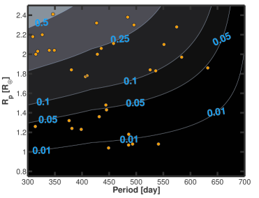
Figure 14 shows the average pipeline completeness contours toward longer $P_{\rm orb}$ for the GK dwarf sample of this study along with the Kepler planet candidate sample in this regime. Using this long period pipeline completeness model and the shorter period PLDF model, we predict the expected planet candidate yield for Kepler. The top panel of Figure 15 shows the difference between observed and predicted planet candidate counts marginalized over 300$<$$P_{\rm orb}$$<$700 days. There is a statistically significant overabundance of planet candidates toward longer periods than predicted from the baseline PLDF derived at the shorter orbital periods. The largest discrepancy is for the smallest $R_{\rm p}$ bin under consideration in Figure 15. The bottom panel of Figure 15 shows the observed minus predicted planet candidate counts as a function of $P_{\rm orb}$ after marginalizing over 0.75$<$$R_{\rm p}$$<$2.5 ${R_{\oplus}}$. The most significant overabundance is in the middle $P_{\rm orb}$ bin. The largest contributor to the overabundance are the cluster of five planet candidates around $R_{\rm p}$$\sim$1.1 ${R_{\oplus}}$ and $P_{\rm orb}$$\sim$500 days that fall along the (0.01) average pipeline completeness contour level.

Figure 14.— Average pipeline completeness contours for the GK dwarf sample toward longer, 300$<$$P_{\rm orb}$$<$700 days, along with the Q1-Q16 Kepler planet candidate sample (orange points).

Figure 15.— Top: marginalized over periods of 300$<$$P_{\rm orb}$$<$700 days observed Kepler planet candidate counts minus the predicted planet candidate counts obtained by extrapolating our planet occurrence rate results from the shorter 50$<$$P_{\rm orb}$$<$300 days analysis of Section VI. Bottom: same as top, but marginalized over planet radius 0.75$<$$R_{\rm p}$$<$2.5 ${R_{\oplus}}$.

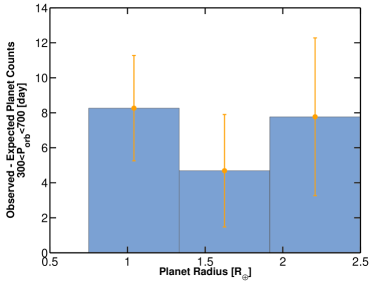
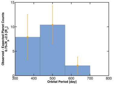
The significant overabundance of planet candidates implies that extrapolations of our PLDF from the 50$<$$P_{\rm orb}$$<$300 days range may underestimate the planet occurrence rates toward longer periods. However, at this time we cannot distinguish between a higher occurrence of planets toward long periods in the Kepler GK dwarf planets, a larger false alarm contribution among the lowest MES planet candidates, or systematic bias in our simplified pipeline completeness model. We are investigating flux time series inversion and permutation tests along with a bootstrap noise characterization test (Seader et al., 2015) in order to calibrate the false alarm rate in the Kepler planet candidate sample.

IX. Terrestrial Planet Occurrence Rate For Venus Orbital Periods

Earth’s sister planet, Venus, has an orbital period within the $P_{\rm orb}$ range of the baseline analysis. Thus, in this section we present results for the occurrence rate of terrestrial planets corresponding to the $P_{\rm orb}$$\sim$0.6 yr of Venus. We define $\zeta_{0.6}$ as the 0.6 yr terrestrial planet occurrence rate, which we take to be within 20% of $R_{\rm p}$=1 ${R_{\oplus}}$ and 20% of $P_{\rm orb}$_♀. The integral range of 20% is within the expectations for the regime of rocky terrestrial planets (Rogers, 2015; Wolfgang & Lopez, 2014). Since $P_{\rm orb}$ is a direct observable, providing occurrence rates in terms of $P_{\rm orb}$  such as $\zeta$, has advantages over providing occurrence rates in terms of stellar insolation flux, such as the Venus zone ($\eta_{\venus}$) concept of Kane et al. (2014) or the HZ ($\eta_{\oplus}$) concept (Kasting et al., 1993; Selsis et al., 2007; Zsom et al., 2013; Kopparapu et al., 2013). Stellar insolation flux is an indirectly measured quantity and $\eta_{\venus}$ and $\eta_{\oplus}$ depend upon uncertain theoretical models for terrestrial planet atmospheric evolution. Providing occurrence rates in terms of $P_{\rm orb}$ facilitates comparison with future Kepler occurrence rate studies and is readily compared to theoretical terrestrial planet formation models.

Figure 16.— Distribution for the 0.6 yr terrestrial planet occurrence rate, $\zeta_{0.6}$, integrated within 20% of $R_{\rm p}$=1 ${R_{\oplus}}$ and $P_{\rm orb}$_♀, using the baseline analysis (filled orange histogram). Solid lines represent results using alternative inputs with the same line types as in Figure 10.

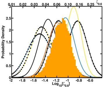
We defer the additional complications in calculating $\eta_{\venus}$ and $\eta_{\oplus}$ to future work. Despite the complications, for G dwarfs, $\zeta_{0.6}$ is a subset of the full $\eta_{\venus}$ parameter space, thus $\zeta_{0.6}$ places a valuable lower limit on $\eta_{\venus}$ for G dwarfs. For the K dwarfs, $P_{\rm orb}$_♀ corresponds to the Sun-Earth insolation flux. Thus, $\zeta_{0.6}$ is a lower limit on the K dwarf $\eta_{\oplus}$. We find $\zeta_{0.6}=0.075$ with an acceptable range of 0.013$\leq\zeta_{0.6}\leq$0.30, and show the baseline and systematic posterior distributions for $\zeta_{0.6}$ in Figure 16.

X. Terrestrial Planet Occurrence Rate For One Year Orbital Periods

X.1. Extrapolating to One Year Orbital Period

The longer, 300$<$$P_{\rm orb}$$<$700 days parameter space roughly coincides with the theoretical HZ for the G dwarf targets, which is a preferred location in a planetary system for a stable water bearing planet (Kasting et al., 1993). In Section VIII, we demonstrated that determining the planet occurrence rate in the 300$<$$P_{\rm orb}$$<$700 days range directly from Kepler data is at a premature stage due to significant false alarm contamination. In this section, we extrapolate our PLDF parametric model in order to calculate two occurrence rate parameters that can be used as a baseline for comparison to future work on refining HZ occurrence rates.

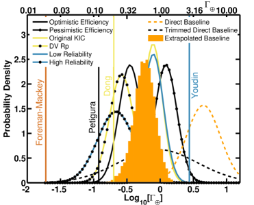
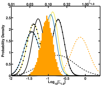
First, we measure the PLDF evaluated at 1.0 ${R_{\oplus}}$ and $P_{\rm orb}$=365.25 days, $\Gamma_{\oplus}=dN/d\ln$$P_{\rm orb}$$d\ln$$R_{\rm p}$ (Youdin, 2011; Foreman-Mackey et al., 2014). In the top panel of Figure 17, we show the baseline (filled orange histogram) $\Gamma_{\oplus}$ determined by extrapolating the PLDF models from the 50$<$$P_{\rm orb}$$<$300 days results. We also show the alternative systematic effects discussed in Section VI.2 (solid curves). Note that the logarithmic scaling for the abscissa indicates substantial systematic uncertainty in the results due to the extrapolation. We also show results for an extrapolated one year terrestrial planet occurrence rate, $\zeta_{1.0}$, defined as the occurrence rate of a planet within 20% of the Earth’s radius and $P_{\rm orb}$ in the bottom panel of Figure 17, for the baseline (filled orange histogram) and alternative systematic effects discussed in Section VI.2 (solid curves). For clarity the effects of eccentricity and for ‘first planet only’ are not displayed in Figure 17 as the results are within the statistical uncertainty of the extrapolated baseline result.

Figure 17.— Top: distribution for the PLDF evaluated at the $R_{\rm p}$ and $P_{\rm orb}$ of Earth, $\Gamma_{\oplus}$, using the extrapolated baseline analysis (filled orange histogram). Solid curves represent results using alternative inputs with the same line types as in Figure 10. We also show two alternative analyses that directly measure, without extrapolation over $P_{\rm orb}$, $\Gamma_{\oplus}$ from the Q1-Q16 Kepler planet candidate sample. The direct measurement of $\Gamma_{\oplus}$ using the full long period planet candidate sample (orange dash curve) and the trimmed long period planet candidate sample (black dash curve) result in higher $\Gamma_{\oplus}$ than the extrapolated PLDF results, respectively. Previous $\Gamma_{\oplus}$ determinations from Foreman-Mackey et al. (2014), Petigura et al. (2013b), Dong & Zhu (2013), and Youdin (2011) are shown with vertical lines as labeled. Bottom: same as top, but for the one year terrestrial planet occurrence rate, $\zeta_{1.0}$.

X.2. Directly Measured At One Year Orbital Period

Though the level of systematics present in our analysis are substantial towards longer periods, we repeat the PLDF parameter estimation in the 0.75$<$$R_{\rm p}$$<$2.5 ${R_{\oplus}}$ and 300$<$$P_{\rm orb}$$<$700 days parameter space. We show the average pipeline completeness for the long period parameter space in Figure 14. The planet candidates from the Q1-Q16 catalog of Mullally et al. (2015) are shown as orange points and are indicated by a binary flag in Table 3. The analysis yields a high $F_{0}=4.7\pm^{3.1}_{1.77}$ planets per star, significantly steeper $\alpha_{\rm avg}=-4.02\pm 0.8$ and shallower $\beta=0.92\pm 0.8$, where the errors are the statistical uncertainty alone.

We defer a more detailed analysis of the systematics to future work, but as a first step we consider culling the planet candidate sample of the five planet candidates along the 0.01 pipeline completeness contour shown in Figure 14. As discussed in Section VIII, this cluster of five planet candidates represents a significant overabundance of planet candidates relative to our shorter period analysis. The overabundance relative to the shorter period extrapolation prediction is nearly erased (1.5-$\sigma$ overabundance), if the cluster of five planet candidates is removed from the sample. The KOIs belonging to the trimmed long period planet candidate sample are indicated by a binary flag in Table 3. The PLDF parameter estimation after removing these five planet candidates yields $F_{0}=1.7\pm^{1.2}_{0.6}$, $\alpha_{\rm avg}=-2.7\pm 1.1$, and $\beta=0.4\pm 0.8$. From this direct analysis we show the one year terrestrial planet occurrence rate in the bottom panel of Figure 17 for $\zeta_{1.0}=0.76\pm^{0.55}_{0.33}$ (orange dash line) and $\zeta_{1.0}=0.21\pm^{0.28}_{0.15}$ (black dash line), evaluated using the full and clipped Kepler planet candidate sample in the 300$<$$P_{\rm orb}$$<$700 days parameter space, respectively.

X.3. One Year Terrestrial Planet Occurrence Rate Summary

The wide range of occurrence rates obtained from this study is a consequence of the difficulties associated with extrapolating, small number statistics, and systematics (including false alarm reliabilities). This will impact refining $\zeta_{1.0}$ and HZ statistics in future studies of the Kepler data set. Compiling our results of the extrapolated and direct analyses, we find $\zeta_{1.0}=0.1$ with an allowed range of 0.01$\leq\zeta_{1.0}\leq$2. Dynamical simulations cannot rule out an upper limit of $\zeta_{1.0}\leq$2 (Smith & Lissauer, 2009). The mutual hill radii separation for a system of three $M_{\rm p}$=1 ${M_{\oplus}}$ planets within the $\zeta_{1.0}$ occurrence region of a G dwarf is $\gtrsim$9 corresponding to $\sim 10^{10}$ yr stability (Smith & Lissauer, 2009). However, for a lower mass K dwarf host and larger ($R_{\rm p}$=1.2${R_{\oplus}}$) planets the mutual hill radii separation $\sim 7$ for a triple planet system in the $\zeta_{1.0}$ zone would likely be unstable on a $10^{9}$ yr timescale.

For the PLDF value at the $R_{\rm p}$ and $P_{\rm orb}$ of Earth, we find $\Gamma_{\oplus}=0.6$ with an acceptable range from 0.04$\leq\Gamma_{\oplus}\leq$11.5. For comparison with previous studies, we show in the bottom panel of Figure 17 as vertical lines estimates of $\Gamma_{\oplus}$ from Foreman-Mackey et al. (2014), Petigura et al. (2013b), Dong & Zhu (2013), and Youdin (2011) from left to right, respectively. In order to calculate results for $\Gamma_{\oplus}$ from the Dong & Zhu (2013) study, we extrapolate their parametric power law model as given for the 1$\leq$$R_{\rm p}$$\leq$2 ${R_{\oplus}}$ analysis from their Table 2. The central value for $\Gamma_{\oplus}$ from Foreman-Mackey et al. (2014) is in tension with our analysis, but there is overlap in the upper tail of their posterior with our lower limits. The analysis of Foreman-Mackey et al. (2014) used the same inputs from Petigura et al. (2013b). However, Foreman-Mackey et al. (2014) determine that finding a steeper fall off of occurrence rates toward longer $P_{\rm orb}$ than Petigura et al. (2013b) and taking into account uncertainty on planet radii lead to a systematically lower value for $\Gamma_{\oplus}$ than Petigura et al. (2013b) when starting from the same inputs. Further work is needed in order to isolate whether the differences between Foreman-Mackey et al. (2014) and our study results predominately from differing inputs or methodology. The other results for $\Gamma_{\oplus}$ from the literature are consistent with our allowed range of $\Gamma_{\oplus}$.

XI. Conclusion

In this study we make use of the first Kepler pipeline run using nearly all (Q1-Q16) the extant Kepler data in order to measure the planet occurrence rate for 0.75$\leq$$R_{\rm p}$$\leq$2.5 ${R_{\oplus}}$in the 50$\leq$$P_{\rm orb}$$\leq$300 days range orbiting the GK dwarf Kepler sample. We employ the first characterization of the Kepler pipeline detection efficiency calibrated with transit injection and recovery tests (Christiansen et al., 2015), the Q1-Q16 Kepler planet candidate catalog (Mullally et al., 2015), and the KIC stellar parameter catalog revision of Huber et al. (2014).

We fit the observed planet candidate sample using a parametric PLDF model following the work of Youdin (2011) and explore alternative inputs into the calculation in order to study the systematic errors present. In general, we find higher occurrence rates for the mini-Neptune to terrestrial planet regime orbiting GK dwarfs and also larger uncertainties driven by the systematics than indicated by previous studies (Dong & Zhu, 2013; Silburt et al., 2015; Petigura et al., 2013a, b; Mulders et al., 2015). We determine that $F_{0}=0.77$ planets per GK dwarf in the Kepler sample have a planet within the 0.75$\leq$$R_{\rm p}$$\leq$2.5 ${R_{\oplus}}$ and 50$\leq$$P_{\rm orb}$$\leq$300 days regime with a systematic dominated allowable range of 0.28$\leq F_{0}\leq$1.9. The power law exponent for the $R_{\rm p}$ dependence in the PLDF model has a best value $\alpha_{\rm avg}$=-1.5 indicating an increasing planet occurrence towards small planets, but the allowed range, -3.25$\leq\alpha_{\rm avg}\leq$0.53, implies that we cannot definitively determine whether the occurrence increases or decreases towards the smallest planets. However, fitting a double power-law model over a wider range of 0.75$\leq$$R_{\rm p}$$\leq$5.0 ${R_{\oplus}}$ does find conclusive evidence for a break in the occurrence rate at $R_{\rm brk}=3.3\pm^{+0.2}_{-0.4}$.

We estimate a one year terrestrial planet occurrence rate, $\zeta_{1.0}=0.1$, with an acceptable range 0.01$\leq\zeta_{1.0}\leq$2, by integrating within 20% of the $R_{\rm p}$ and $P_{\rm orb}$ of Earth. The narrower $\zeta_{1.0}$ parameter space is a subset of the G dwarf HZ, $\eta_{\oplus}$ (Kasting et al., 1993; Selsis et al., 2007; Zsom et al., 2013; Kopparapu et al., 2013). Thus, $\zeta_{1.0}$ places a lower limit on $\eta_{\oplus}$ for G dwarfs. $\zeta_{1.0}$, which depends upon the direct observable $P_{\rm orb}$, facilitates comparison with future Kepler occurrence rate studies and is readily compared to theoretical terrestrial planet formation models. We defer estimates of $\eta_{\oplus}$, which depends upon the indirect observable of stellar insolation and uncertain atmospheric evolution theory for terrestrial planets outside the Solar System, to future studies.

We also determine a 0.6 year terrestrial planet occurrence rate, $\zeta_{0.6}$=0.075, with an acceptable range 0.013$\leq\zeta_{0.6}\leq$0.30, by integrating within 20% of the $R_{\rm p}$=1 ${R_{\oplus}}$ and $P_{\rm orb}$_♀ corresponding to Venus-type planets for G dwarf hosts. For the K dwarfs of our sample (${T_{\rm eff}}$$<$5200 K), $P_{\rm orb}$=0.6 yr roughly corresponds to the Solar-Earth insolation flux level. Thus, $\zeta_{0.6}$ places a lower limit on $\eta_{\oplus}$ for K dwarfs.

Although the current results are dominated by systematic uncertainties, which, unlike statistical uncertainties that are limited by the quantity and quality of data, can be minimized with additional study. From our analysis, we identify the leading sources of systematics: instrumental false alarm contamination of the planet candidate sample, determining planet radii (independent of the degeneracy with ${R_{\star}}$), pipeline completeness, and stellar parameters. Additional work on third light contamination, orbital eccentricity, astrophysical false positives, and false negative rate of the planet vetting process is needed. All of these should be examined carefully before accepting a definitive value for $\eta_{\oplus}$.

References

- Allen (2007) Allen, P. R. 2007, ApJ, 668, 492
- Baddeley (2007) Baddeley, A. J. 2007, Lecture Notes in Mathematics: Stochastic Geometry, (Springer Verlag, Berlin, Germany)
- Ballard et al. (2011) Ballard, S., Fabrycky, D., Fressin, F., et al. 2011, ApJ, 743, 200
- Batalha (2014) Batalha, N. M. 2014, Proceedings of the National Academy of Science, 111, 12647
- Batalha et al. (2013) Batalha, N. M., Rowe, J. F., Bryson, S. T., et al. 2013, ApJS, 204, 24
- Bayliss & Sackett (2011) Bayliss, D. D. R., & Sackett, P. D. 2011, ApJ, 743, 103
- Benz et al. (2014) Benz, W., Ida, S., Alibert, Y., Lin, D., & Mordasini, C. 2014, Protostars and Planets VI, 691
- Bonfils et al. (2013) Bonfils, X., Delfosse, X., Udry, S., et al. 2013, A&A, 549, A109
- Borucki et al. (2010) Borucki, W. J., Koch, D., Basri, G., et al. 2010, Science, 327, 977
- Borucki et al. (2011a) Borucki, W. J., Koch, D. G., Basri, G., et al. 2011a, ApJ, 728, 117
- Borucki et al. (2011b) Borucki, W. J., Koch, D. G., Basri, G., et al. 2011b, ApJ, 736, 19
- Borucki et al. (2012) Borucki, W. J., Koch, D. G., Batalha, N., et al. 2012, ApJ, 745, 120
- Bowler et al. (2010) Bowler, B. P., Johnson, J. A., Marcy, G. W., et al. 2010, ApJ, 709, 396
- Brown et al. (2011) Brown, T. M., Latham, D. W., Everett, M. E., & Esquerdo, G. A. 2011, AJ, 142, 112
- Burke et al. (2006) Burke, C. J., Gaudi, B. S., DePoy, D. L., & Pogge, R. W. 2006, AJ, 132, 210
- Burke et al. (2007) Burke, C. J., McCullough, P. R., Valenti, J. A., et al. 2007, ApJ, 671, 2115
- Burke (2008) Burke, C. J. 2008, ApJ, 679, 1566
- Burke et al. (2010) Burke, C. J., McCullough, P. R., Bergeron, L. E., et al. 2010, ApJ, 719, 1796
- Burke et al. (2014) Burke, C. J., Bryson, S. T., Mullally, F., et al. 2014, ApJS, 210, 19
- Burke & McCullough (2014) Burke, C. J., & McCullough, P. R. 2014, ApJ, 792, 79
- Burke et al. (2015) Burke, C. J., Mullally, F., Christiansen, J., et al. 2015, American Astronomical Society Meeting Abstracts, 225, #122.04
- Butler et al. (2006) Butler, R. P., Wright, J. T., Marcy, G. W., et al. 2006, ApJ, 646, 505
- Cartier et al. (2014) Cartier, K. M. S., Gilliland, R. L., Wright, J. T., & Ciardi, D. R. 2014, arXiv:1407.1057
- Catanzarite & Shao (2011) Catanzarite, J., & Shao, M. 2011, ApJ, 738, 151
- Charbonneau et al. (2009) Charbonneau, D., Berta, Z. K., Irwin, J., et al. 2009, Nature, 462, 891
- Christiansen et al. (2012) Christiansen, J. L., Jenkins, J. M., Caldwell, D. A., et al. 2012, PASP, 124, 1279
- Christiansen et al. (2013) Christiansen, J. L., Clarke, B. D., Burke, C. J., et al. 2013, ApJS, 207, 35
- Christiansen et al. (2015) Christiansen, J. L., et al. 2015, ApJ, submitted
- Ciardi et al. (2015) Ciardi, D. R., Beichman, C. A., Horch, E. P., & Howell, S. B. 2015, arXiv:1503.03516
- Clanton & Gaudi (2014) Clanton, C., & Gaudi, B. S. 2014, ApJ, 791, 91
- Claret & Bloemen (2011) Claret, A., & Bloemen, S. 2011, A&A, 529, AA75
- Coughlin et al. (2014) Coughlin, J. L., Thompson, S. E., Bryson, S. T., et al. 2014, AJ, 147, 119
- Coughlin et al. (2015) Coughlin, J., Mullally, F., Thompson, S. E., & Kepler Team 2015, American Astronomical Society Meeting Abstracts, 225, #202.05
- Cumming et al. (2008) Cumming, A., Butler, R. P., Marcy, G. W., et al. 2008, PASP, 120, 531
- Daley & Vere-Jones (1988) Daley, D. J., & Vere-Jones, D. 1988, An Introduction to the Theory of Point Processes, Vol. 1 (Springer, New York, NY)
- Deeg et al. (2004) Deeg, H. J., Alonso, R., Belmonte, J. A., et al. 2004, PASP, 116, 985
- Désert et al. (2015) Désert, J.-M., Charbonneau, D., Torres, G., et al. 2015, arXiv:1503.03173
- Dong & Zhu (2013) Dong, S., & Zhu, Z. 2013, ApJ, 778, 53
- Dotter et al. (2008) Dotter, A., Chaboyer, B., Jevremović, D., et al. 2008, ApJS, 178, 89
- Drake (2013) Drake, F. 2013, International Journal of Astrobiology, 12, 173
- Dressing & Charbonneau (2013) Dressing, C. D., & Charbonneau, D. 2013, ApJ, 767, 95
- Dressing & Charbonneau (2015) Dressing, C. D., & Charbonneau, D. 2015, arXiv:1501.01623
- Everett et al. (2013) Everett, M. E., Howell, S. B., Silva, D. R., & Szkody, P. 2013, ApJ, 771, 107
- Farr et al. (2014) Farr, W. M., Mandel, I., Aldridge, C., & Stroud, K. 2014, arXiv:1412.4849
- Fischer & Valenti (2005) Fischer, D. A., & Valenti, J. 2005, ApJ, 622, 1102
- Foreman-Mackey et al. (2014) Foreman-Mackey, D., Hogg, D. W., & Morton, T. D. 2014, ApJ, 795, 64
- Fressin et al. (2013) Fressin, F., Torres, G., Charbonneau, D., et al. 2013, ApJ, 766, 81
- Gaidos & Mann (2013) Gaidos, E., & Mann, A. W. 2013, ApJ, 762, 41
- Gaudi (2000) Gaudi, B. S. 2000, ApJ, 539, L59
- Gilliland et al. (2000) Gilliland, R. L., Brown, T. M., Guhathakurta, P., et al. 2000, ApJ, 545, L47
- Gilliland et al. (2011) Gilliland, R. L., Chaplin, W. J., Dunham, E. W., et al. 2011, ApJS, 197, 6
- Giménez (2006) Giménez, A. 2006, A&A, 450, 1231
- Gould et al. (2006) Gould, A., Dorsher, S., Gaudi, B. S., & Udalski, A. 2006, Actaa, 56, 1
- Gregory (2005) Gregory, P. C. 2005, Bayesian Logical Data Analysis for the Physical Sciences: A Comparative Approach with ‘Mathematica’ Support (Cambridge University Press, Cambridge, UK)
- Hartman et al. (2009) Hartman, J. D., Gaudi, B. S., Holman, M. J., et al. 2009, ApJ, 695, 336
- Holman et al. (2006) Holman, M. J., Winn, J. N., Latham, D. W., et al. 2006, ApJ, 652, 1715
- Howard et al. (2010) Howard, A. W., Marcy, G. W., Johnson, J. A., et al. 2010, Science, 330, 653
- Howard et al. (2012) Howard, A. W., Marcy, G. W., Bryson, S. T., et al. 2012, ApJS, 201, 15
- Huber et al. (2014) Huber, D., Silva Aguirre, V., Matthews, J. M., et al. 2014, ApJS, 211, 2
- Ida & Lin (2004) Ida, S., & Lin, D. N. C. 2004, ApJ, 604, 388
- Jenkins (2002) Jenkins, J. M. 2002, ApJ, 575, 493
- Jenkins et al. (2002) Jenkins, J. M., Caldwell, D. A., & Borucki, W. J. 2002, ApJ, 564, 495
- Kane et al. (2014) Kane, S. R., Kopparapu, R. K., & Domagal-Goldman, S. D. 2014, ApJ, 794, LL5
- Kasting et al. (1993) Kasting, J. F., Whitmire, D. P., & Reynolds, R. T. 1993, Icarus, 101, 108
- Kipping (2014) Kipping, D. M. 2014, MNRAS, 444, 2263
- Koch et al. (2010) Koch, D. G., Borucki, W. J., Basri, G., et al. 2010, ApJ, 713, LL79
- Kopparapu et al. (2013) Kopparapu, R. K., Ramirez, R., Kasting, J. F., et al. 2013, ApJ, 765, 131
- Kouveliotou et al. (2014) Kouveliotou, C., Agol, E., Batalha, N., et al. 2014, arXiv:1401.3741
- Kraus & Hillenbrand (2012) Kraus, A. L., & Hillenbrand, L. A. 2012, ApJ, 757, 141
- Leger et al. (2015) Leger, A., Defrere, D., Malbet, F., Labadie, L., & Absil, O. 2015, arXiv:1504.08232
- Lillo-Box et al. (2014) Lillo-Box, J., Barrado, D., & Bouy, H. 2014, A&A, 566, AA103
- Loredo (1992) Loredo, T. J. 1992, Statistical Challenges in Modern Astronomy, 275 (New York: Springer-Verlag)
- Mandel & Agol (2002) Mandel, K., & Agol, E. 2002, ApJ, 580, L171
- Mann et al. (2012) Mann, A. W., Gaidos, E., Lépine, S., & Hilton, E. J. 2012, ApJ, 753, 90
- Marcy et al. (2005) Marcy, G., Butler, R. P., Fischer, D., et al. 2005, Progress of Theoretical Physics Supplement, 158, 24
- Mayor et al. (2011) Mayor, M., Marmier, M., Lovis, C., et al. 2011, arXiv:1109.2497
- McCauliff et al. (2014) McCauliff, S., Jenkins, J. M., Catanzarite, J., et al. 2014, arXiv:1408.1496
- Meibom et al. (2013) Meibom, S., Torres, G., Fressin, F., et al. 2013, Nature, 499, 55
- Morton & Johnson (2011) Morton, T. D., & Johnson, J. A. 2011, ApJ, 738, 170
- Morton (2012) Morton, T. D. 2012, ApJ, 761, 6
- Morton & Swift (2014) Morton, T. D., & Swift, J. 2014, ApJ, 791, 10
- Mordasini et al. (2015) Mordasini, C., Mollière, P., Dittkrist, K.-M., Jin, S., & Alibert, Y. 2015, International Journal of Astrobiology, 14, 201
- Muirhead et al. (2012) Muirhead, P. S., Hamren, K., Schlawin, E., et al. 2012, ApJ, 750, LL37
- Mulders et al. (2015) Mulders, G. D., Pascucci, I., & Apai, D. 2015, ApJ, 798, 112
- Mullally et al. (2015) Mullally, F., Coughlin, J. L., Thompson, S. E., et al. 2015, arXiv:1502.02038
- Naef et al. (2005) Naef, D., Mayor, M., Beuzit, J.-L., et al. 2005, 13th Cambridge Workshop on Cool Stars, Stellar Systems and the Sun, 560, 833
- Nielsen et al. (2014) Nielsen, E. L., Liu, M. C., Wahhaj, Z., et al. 2014, American Astronomical Society Meeting Abstracts #223, 223, #348.19
- Petigura et al. (2013a) Petigura, E. A., Marcy, G. W., & Howard, A. W. 2013, ApJ, 770, 69
- Petigura et al. (2013b) Petigura, E. A., Howard, A. W., & Marcy, G. W. 2013, Proceedings of the National Academy of Science, 110, 19273
- Pinsonneault et al. (2012) Pinsonneault, M. H., An, D., Molenda-Żakowicz, J., et al. 2012, ApJS, 199, 30
- Prantzos (2013) Prantzos, N. 2013, International Journal of Astrobiology, 12, 246
- Rogers (2015) Rogers, L. A. 2015, ApJ, 801, 41
- Rowe et al. (2014) Rowe, J. F., Bryson, S. T., Marcy, G. W., et al. 2014, ApJ, 784, 45
- Rowe et al. (2015) Rowe, J. F., Coughlin, J. L., Antoci, V., et al. 2015, ApJS, 217, 16
- Rowe et al. (2015) Rowe, J., Barclay, T., Batalha, N. M., et al. 2015, American Astronomical Society Meeting Abstracts, 225, #105.06
- Sahu et al. (2006) Sahu, K. C., Casertano, S., Bond, H. E., et al. 2006, Nature, 443, 534
- Santerne et al. (2012) Santerne, A., Díaz, R. F., Moutou, C., et al. 2012, A&A, 545, AA76
- Seader et al. (2013) Seader, S., Tenenbaum, P., Jenkins, J. M., & Burke, C. J. 2013, ApJS, 206, 25
- Seader et al. (2014) Seader, S., Tenenbaum, P., Burke, C. J., & Jenkins, J. M. 2014, American Astronomical Society Meeting Abstracts #224, 224, #120.03
- Seader et al. (2015) Seader, S., Jenkins, J. M., Tenenbaum, P., et al. 2015, ApJS, 217, 18
- Seager & Mallén-Ornelas (2003) Seager, S., & Mallén-Ornelas, G. 2003, ApJ, 585, 1038
- Selsis et al. (2007) Selsis, F., Kasting, J. F., Levrard, B., et al. 2007, A&A, 476, 1373
- Silburt et al. (2015) Silburt, A., Gaidos, E., & Wu, Y. 2015, ApJ, 799, 180
- Smith & Lissauer (2009) Smith, A. W., & Lissauer, J. J. 2009, Icarus, 201, 381
- Smith et al. (2012) Smith, J. C., Stumpe, M. C., Van Cleve, J. E., et al. 2012, PASP, 124, 1000
- Southworth (2011) Southworth, J. 2011, MNRAS, 417, 2166
- Stark et al. (2015) Stark, C. C., Roberge, A., Mandell, A., et al. 2015, arXiv:1506.01723
- Stumpe et al. (2012) Stumpe, M. C., Smith, J. C., Van Cleve, J. E., et al. 2012, PASP, 124, 985
- Tabachnik & Tremaine (2002) Tabachnik, S., & Tremaine, S. 2002, MNRAS, 335, 151
- Tenenbaum et al. (2012) Tenenbaum, P., Christiansen, J. L., Jenkins, J. M., et al. 2012, ApJS, 199, 24
- Tenenbaum et al. (2013) Tenenbaum, P., Jenkins, J. M., Seader, S., et al. 2013, ApJS, 206, 5
- Tenenbaum et al. (2014) Tenenbaum, P., Jenkins, J. M., Seader, S., et al. 2014, ApJS, 211, 6
- Torres et al. (2008) Torres, G., Winn, J. N., & Holman, M. J. 2008, ApJ, 677, 1324
- Traub (2012) Traub, W. A. 2012, ApJ, 745, 20
- van Saders & Gaudi (2011) van Saders, J. L., & Gaudi, B. S. 2011, ApJ, 729, 63
- von Braun et al. (2009) von Braun, K., Kane, S. R., & Ciardi, D. R. 2009, ApJ, 702, 779
- Weldrake & Sackett (2005) Weldrake, D. T. F., & Sackett, P. D. 2005, ApJ, 620, 1033
- Wolfgang & Lopez (2014) Wolfgang, A., & Lopez, E. 2014, arXiv:1409.2982
- Wu et al. (2010) Wu, H., Twicken, J. D., Tenenbaum, P., et al. 2010, Proc. SPIE, 7740, 774019
- Wright et al. (2012) Wright, J. T., Marcy, G. W., Howard, A. W., et al. 2012, ApJ, 753, 160
- Youdin (2011) Youdin, A. N. 2011, ApJ, 742, 38
- Zsom et al. (2013) Zsom, A., Seager, S., de Wit, J., & Stamenković, V. 2013, ApJ, 778, 109