Mixtures of Multivariate Power Exponential Distributions

Abstract

An expanded family of mixtures of multivariate power exponential distributions is introduced. While fitting heavy-tails and skewness has received much attention in the model-based clustering literature recently, we investigate the use of a distribution that can deal with both varying tail-weight and peakedness of data. A family of parsimonious models is proposed using an eigen-decomposition of the scale matrix. A generalized expectation-maximization algorithm is presented that combines convex optimization via a minorization-maximization approach and optimization based on accelerated line search algorithms on the Stiefel manifold. Lastly, the utility of this family of models is illustrated using both toy and benchmark data.

1 Introduction

Mixture models have become the most popular methodology to investigate heterogeneity in data (cf. Titterington et al., 1985; McLachlan and Peel, 2000b). Model-based learning makes use of mixture models to partition data points. Model-based clustering and classification refer to the scenarios where observations have no known labels and some known labels, respectively, a priori. The number of these partitions or clusters may or may not be known in advance. While approaches based on mixtures of Gaussian distributions (e.g., Banfield and Raftery, 1993; Celeux and Govaert, 1995) remain popular for model-based clustering, these algorithms are susceptible to performing poorly in the presence of outliers. As a result, more robust mixtures of distributions are becoming increasingly popular. Some of these mixtures aim to tackle tail-weight (e.g., Andrews and McNicholas, 2011, 2012; Forbes and Wraith, 2014), some deal with skewness (e.g., Lin et al., 2007; Franczak et al., 2014), while others account for both (e.g., Karlis and Santourian, 2009; Subedi and McNicholas, 2014; Vrbik and McNicholas, 2014; Browne and McNicholas, 2015).

Herein, we utilize a family of mixture models based on the multivariate power exponential (MPE) distribution (Gómez et al., 1998). This distribution is sometimes also called the multivariate generalized Gaussian distribution. Depending on the shape parameter $\beta$, two kinds of distributions can be obtained: for $0<\beta<1$ a leptokurtic distribution is obtained, which is characterized by a thinner peak and heavy tails compared to the Gaussian distribution; whereas, for $\beta>1$, a platykurtic distribution is obtained, which is characterized by a flatter peak and thin tails compared to the Gaussian distribution. The distribution is quite flexible: for $\beta=0.5$, we have a Laplace (double-exponential) distribution and, for $\beta=1$, we have a Gaussian distribution. Furthermore, when $\beta\rightarrow\infty$ the MPE becomes a multivariate uniform distribution.

Figure 1: Density plots for different values of $\beta$. The MPE distribution is quite flexible: for $\beta=0.5$, we have a Laplace (double-exponential) distribution and for $\beta=1$, we have a Gaussian distribution. Furthermore, as $\beta\rightarrow\infty$, the MPE distribution becomes a multivariate uniform distribution.

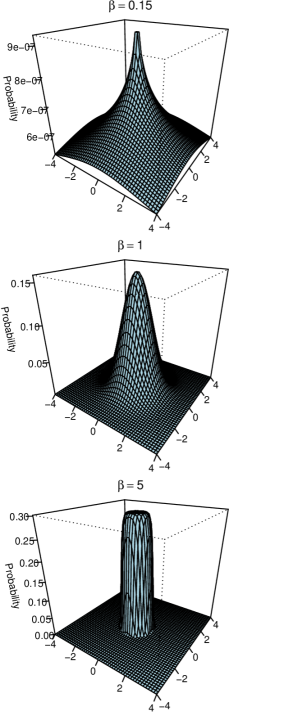
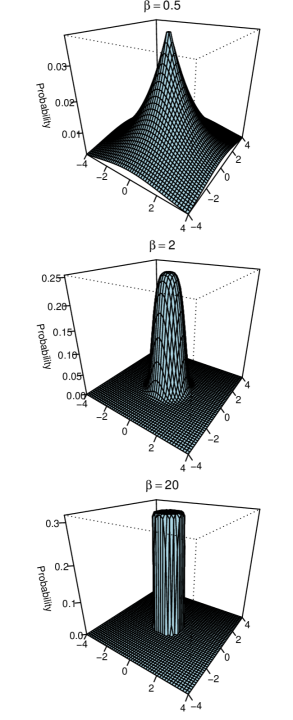
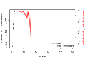
The MPE distribution has been used in many different applications (Lindsey, 1999; Cho and Bui, 2005; Verdoolaege et al., 2008). However, due to difficulties in estimating the covariance over the entire support of the shape parameter $\beta\in(0,\infty)$, its potential has not yet been fully explored. This distribution presents a difficult parameter estimation problem because none of the parameter estimates are available in closed form. Previously proposed estimation strategies have included optimization based on geodesic convexity for unconstrained covariance matrices (Zhang et al., 2013) and Newton-Raphson recursions (Pascal et al., 2013). Some work with this distribution has focused on the special case where $0<\beta<1$ (Gómez-Sánchez-Manzano et al., 2008; Bombrun et al., 2012; Pascal et al., 2013). However, for imposing parsimony in a traditional model-based clustering context (through different constraints on terms of specific decompositions of the component scale, or covariance, matrices), these methods are not ideal. Previously, a family of five models based on mixtures of MPE distributions has been used for robust clustering (Zhang and Liang, 2010). This work made use of fixed point iterations for the special case where $0<\beta<2$ (see Appendix A). Within $0<\beta<2$, the fixed point algorithm converges; however, it yields monotonic improvements in log-likelihood only for $0<\beta\leq 1$. For $\beta\geq 2$, this fixed point algorithm is guaranteed to diverge, which leads to (negative) infinite log-likelihood values.

Herein, a generalized expectation-maximization (GEM; Dempster et al., 1977) strategy is proposed and illustrated. This algorithm works for $0<\beta<\infty$. This estimation procedure also guarantees monotonicity of the log-likelihood. We make use of MM algorithms (Hunter and Lange, 2000) and accelerated line search algorithms on the Stiefel manifold (Absil et al., 2009; Browne and McNicholas, 2014b). This allows for the estimation of a wide range of constrained models, and a family of sixteen MPE mixture models is presented. These models can account for varying tail weight and peakedness of mixture components. In Section 2, we summarize the MPE distribution. Section 3 gives a GEM algorithm for parameter estimation. Section 4 investigates the performance of the family of mixture models on toy and benchmark data. We conclude with a discussion and suggest some avenues for further research in Section 5.

2 Multivariate Power Exponential Distribution

A random vector $\boldsymbol{X}$ follows a $p$-dimensional power exponential distribution (Landsman and Valdez, 2003) if the density is of the form

$$h(\boldsymbol{x}|\mbox{\boldmath$\mu$},\mbox{\boldmath$\Sigma$},r,s)=c_{p}|\mbox{\boldmath$\Sigma$}|^{-\frac{1}{2}}\exp\left\{-\frac{r}{2^{s}}\delta(\boldsymbol{x})^{s}\right\},$$ (1)

where

$$c_{p}=\frac{s\Gamma\left(\frac{p}{2}\right)}{(2\pi)^{p/2}\Gamma\left(\frac{p}{2s}\right)}r^{p/(2s)},$$

$\delta(\boldsymbol{x}):=\delta\left(\boldsymbol{x}|\mbox{\boldmath$\mu$},\mbox{\boldmath$\Sigma$}\right)=\left(\boldsymbol{x}-\mbox{\boldmath$\mu$}\right)^{\prime}\mbox{\boldmath$\Sigma$}^{-1}\left(\boldsymbol{x}-\mbox{\boldmath$\mu$}\right)$, $\mu$ and $\Sigma$ are the location parameter (also the mean) and positive-definite scale matrix, respectively, and $r,s>0$. This elliptical distribution is a multivariate Kotz-type distribution. However, it has identifiability issues concerning $\Sigma$ and $r$: the density with $\mbox{\boldmath$\Theta$}=\{\mbox{\boldmath$\mu$},\mbox{\boldmath$\Sigma$}^{*},r^{*},s\}$, where $\mbox{\boldmath$\Sigma$}^{*}=\mbox{\boldmath$\Sigma$}/2$ and $r^{*}=r/2^{s}$, is the same as (1).

Using the parametrization given by Gómez et al. (1998), a random vector $\boldsymbol{X}$ follows a $p$-dimensional power exponential distribution if the density is

$$f(\boldsymbol{x}|\mbox{\boldmath$\mu$},\mbox{\boldmath$\Sigma$},\beta)=k|\mbox{\boldmath$\Sigma$}|^{-\frac{1}{2}}\exp\left\{-\frac{1}{2}\delta(\boldsymbol{x})^{\beta}\right\},$$ (2)

where

$$k=\frac{p\Gamma\left(\frac{p}{2}\right)}{\pi^{p/2}\Gamma\left(1+\frac{p}{2\beta}\right)2^{1+\frac{p}{2\beta}}},$$

$\delta(\boldsymbol{x}):=\delta\left(\boldsymbol{x}|\mbox{\boldmath$\mu$},\mbox{\boldmath$\Sigma$}\right)=\left(\boldsymbol{x}-\mbox{\boldmath$\mu$}\right)^{\prime}\mbox{\boldmath$\Sigma$}^{-1}\left(\boldsymbol{x}-\mbox{\boldmath$\mu$}\right)$, $\mu$ is the location parameter (also the mean), $\Sigma$ is a positive-definite scale matrix, and $\beta$ determines the kurtosis. Moreover, it is a special parameterization of the MPE distribution given in (1), with $r=2^{\beta-1}$ and $s=\beta$. The covariance and multidimensional kurtosis coefficient for this distribution are

$$\text{Cov}(\boldsymbol{X})=\frac{2^{1/\beta}\Gamma\left(\frac{p+2}{2\beta}\right)}{p\Gamma\left(\frac{p}{2\beta}\right)}\mbox{\boldmath$\Sigma$}$$ (3)

and

$$\gamma_{2}(\boldsymbol{X})=\frac{p^{2}\Gamma\left(\frac{p}{2\beta}\right)\Gamma\left(\frac{p+4}{2\beta}\right)}{\Gamma^{2}\left(\frac{p+2}{2\beta}\right)}-p(p+2),$$ (4)

respectively (Gómez et al., 1998). Here, $\gamma_{2}(\boldsymbol{X})$ denotes the multidimensional kurtosis coefficient that is defined as

$$\mathbb{E}\left\{\left[(\boldsymbol{X}-\mbox{\boldmath$\mu$})^{\prime}\text{Var}(\boldsymbol{X})^{-1}(\boldsymbol{X}-\mbox{\boldmath$\mu$})\right]^{2}\right\}-p(p+2)$$

(Mardia et al., 1980; Gómez et al., 1998). For $\beta\in(0,1)$, the MPE distribution is a scale mixture of Gaussian distributions (Gómez-Sánchez-Manzano et al., 2008).

Based on the MPE distribution, a mixture model can conveniently be defined as

$$g(\boldsymbol{x}|\mbox{\boldmath$\Theta$})=\sum_{g=1}^{G}\pi_{g}f\left(\boldsymbol{x}|\mbox{\boldmath$\mu$}_{g},\mbox{\boldmath$\Sigma$}_{g},\beta_{g}\right),$$

where $f(\cdot)$ is the $g$th component density and $\Theta$ denotes all parameters. Here, $\mbox{\boldmath$\mu$}_{g}$, $\mbox{\boldmath$\Sigma$}_{g}$, and $\beta_{g}$ denote the mean, scale matrix, and shape parameter, respectively, of the $g$th component. Here, $\pi_{1},\ldots,\pi_{G}$ are the mixing weights such that $\pi_{g}>0$ ($g=1,\ldots,G$) and $\sum^{G}_{g=1}\pi_{g}=1$. Note that mixtures of MPE distributions have previously been shown to be identifiable (Zhang and Liang, 2010).

Because the number of parameters in the scale matrix increases quadratically with data dimensionality, it is common practice to impose a decomposition that allows for reduction in the number of parameters to be estimated. An eigen-decomposition decomposes a component covariance matrix into the form $\mbox{\boldmath$\Sigma$}_{g}=\lambda_{g}{\mbox{\boldmath$\Gamma$}_{g}}{\mbox{\boldmath$\Delta$}_{g}}{\mbox{\boldmath$\Gamma$}_{g}}^{\prime}$, where $\lambda_{g}$, $\mbox{\boldmath$\Gamma$}_{g}$, and $\mbox{\boldmath$\Delta$}_{g}$ can be interpreted geometrically (Banfield and Raftery, 1993). Specifically, $\mbox{\boldmath$\Delta$}_{g}$ is a diagonal matrix with entries proportional to the eigenvalues of $\mbox{\boldmath$\Sigma$}_{g}$ (with $|\boldsymbol{\Delta}_{g}|=1$), $\lambda_{g}$ is the associated constant of proportionality, and $\boldsymbol{\Gamma}_{g}$ is a $p\times p$ orthogonal matrix of the eigenvectors of $\mbox{\boldmath$\Sigma$}_{g}$ (with entries ordered according to the eigenvalues). Constraining these terms to be equal or variable across groups allows for a family of fourteen parsimonious mixture models (Celeux and Govaert, 1995). In this paper, we work with a subset of eight parsimonious models (EII, VII, EEI, VVI, EEE, EEV, VVE, and VVV), including the most parsimonious (EII) and the fully unconstrained (VVV) models (Table 1). In addition, there is the option to constrain $\beta_{g}$ to be equal across groups. This option, together with the covariances structures, results in a family of sixteen models. The nomenclature for this family is a natural extension of that used for the covariance structures, e.g., the model with a VVI scale structure and $\beta_{g}$ constrained to be equal across groups is denoted VVIE. This family of models is referred to as the ePEM (eigen-decomposed power exponential mixture) family hereafter.

Table 1: Nomenclature, scale matrix structure, and the number of free scale parameters for the ePEM family of models.

Model	$\lambda_{g}$	$\mbox{\boldmath$\Delta$}_{g}$	$\mbox{\boldmath$\Gamma$}_{g}$	$\boldsymbol{\Sigma}_{g}$	Free Cov. Parameters
EII	Equal	Spherical	-	$\lambda\boldsymbol{I}$	1
VII	Variable	Spherical	-	$\lambda_{g}\boldsymbol{I}$	$G$
EEI	Equal	Equal	Axis-Aligned	$\lambda\boldsymbol{\Delta}$	$p$
VVI	Variable	Variable	Axis-Aligned	$\lambda_{g}\boldsymbol{\Delta}_{g}$	$Gp$
EEE	Equal	Equal	Equal	$\lambda\boldsymbol{\Gamma}\boldsymbol{\Delta}\boldsymbol{\Gamma}^{\prime}$	$p\left(p+1\right)/2$
EEV	Equal	Equal	Variable	$\lambda\boldsymbol{\Gamma}_{g}\boldsymbol{\Delta}\boldsymbol{\Gamma}_{g}^{\prime}$	$Gp(p+1)/2-(G-1)p$
VVE	Variable	Variable	Equal	$\lambda_{g}\boldsymbol{\Gamma}\boldsymbol{\Delta}_{g}\boldsymbol{\Gamma}^{\prime}$	$p(p+1)/2+(G-1)p$
VVV	Variable	Variable	Variable	$\lambda_{g}\boldsymbol{\Gamma}_{g}\boldsymbol{\Delta}_{g}\boldsymbol{\Gamma}_{g}^{\prime}$	$Gp\left(p+1\right)/2$

3 Inference

The expectation-maximization (EM) algorithm (Dempster et al., 1977) is an iterative procedure based on the complete-data likelihood. At each iteration, the the expected value of the complete-data log-likelihood is maximized to yield updates for the parameters of interest. The expectation-conditional-maximization (ECM) algorithm (Meng and Rubin, 1993) replaces the maximization step of the EM algorithm with a number of conditional maximization (CM) steps. This might be necessary due to the form of the likelihood or because the conditional maximization steps are less computationally expensive. In our parameter estimation algorithm, CM steps are used within a framework that increases, rather than maximizes, the expected value of the complete data log-likelihood at each iteration. Such an approach, i.e., one that has the latter feature, is called a GEM algorithm. The parameter updates associated with our GEM algorithm are given in Appendix B.

4 Results

For our numerical analyses, we use the Bayesian information criterion (BIC; Schwarz, 1978) and the integrated complete likelihood (ICL; Biernacki et al., 2000) for model selection. A stopping criterion based on the Aitken acceleration (Aitken, 1926) is used to determine convergence and the adjusted Rand index (ARI; Hubert and Arabie, 1985) is used for performance assessment. More details are in Appendix C. In Appendix A, we compare the performance of our algorithm to an algorithm based on fixed point iterations.

4.1 Simulations

For simulating from the MPE distribution, a modified version of the function rmvpowerexp from package MNM (Nordhausen and Oja, 2011) in R (R Core Team, 2013) is used. The function was modified due to a typo in the rmvpowerexp code. This program utilizes the stochastic representation of the MPE distribution (Gómez et al., 1998) to generate data. This works quite well in lower dimensions. In higher dimensions, a Metropolis-Hastings-based simulation rule can easily be constructed. We illustrate the performance of our family of models using simulations in a wide range of scenarios: for light-tailed components, for light- and heavy-tailed components, for data simulated from Gaussian and $t$-distributions, for higher-dimensional data, and for low overall sample size. When data are simulated from the MPE distribution only, we also show parameter recovery. For comparison to existing mixture models based on elliptically contoured distributions, the mixture (Browne et al., 2014) and teigen (Andrews and McNicholas, 2014) packages in R are employed. These packages implement mixtures of Gaussian and mixtures of multivariate Student-t distributions, respectively. To facilitate a direct comparison, we restrict mixture and teigen to the analogues of the ePEM models (Table 1). Note that we use the mixture package rather than mclust (Fraley et al., 2012) because the VVE model is available within mixture but not within mclust, which only implements ten of the 14 models of Celeux and Govaert (1995). Moreover, as compared to Rmixmod (Lebret et al., 2012), certain models in the mixture family are better optimized for higher dimensions (cf. Browne and McNicholas, 2014a). Note that the teigen package additionally allows for constraining of the degrees of freedom parameter ($\nu$). Hence, a VVIV model implies that $\lambda_{g}$, $\mbox{\boldmath$\Delta$}_{g}$, and $\nu_{g}$ are different between groups, and $\mbox{\boldmath$\Gamma$}_{g}$ is the identity matrix. Note that the same starting values are used for all three algorithms, i.e., for each $G$, the initial $\tau_{ig}$ are selected from the best $k$-means clustering results from ten random starting values for the $k$-means algorithm (Hartigan and Wong, 1979).

Simulation 1: Two light-tailed components

A two-component mixture is simulated with 450 observations with the sample sizes for each group sampled from a binomial distribution with success probability $0.45$. The first component is simulated from a two-dimensional MPE distribution with zero mean, identity scale matrix, and $\beta_{1}=2$. The second component is simulated from a two-dimensional MPE distribution with mean $(2,0)^{\prime}$, identity scale matrix, and $\beta_{2}=5$. Note that this corresponds to an EIIV model. The simulated components are not well separated. All three algorithms are run on 100 such data sets. For the ePEM family, a two-component model is selected by the BIC (and the ICL) for each of the 100 data sets. On the other hand, for the mixture family, the BIC selects a two-component model 77 times, and three, four, and five component models are selected 15, 6, and 2 times, respectively. Similarly, for the teigen family, two, three, four, and five component models are selected 61, 10, 26, and 3 times, respectively. Clearly, for both of the latter families, more components are being fitted to deal with the light-tailed nature of the data.

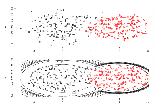
For the ePEM family, the EIIV model is selected by the BIC 97 times out of 100, with the VIIE model selected the other 3 times. The ARI values for the selected ePEM models range from 0.81 to 0.95, with a median (mean) ARI value of 0.88 (0.88). The selected mixture models yield ARI values ranging between 0.30 and 0.96, with a median (mean) value of 0.85 (0.79). Similarly, the teigen family yields ARI values ranging between 0.29 and 0.94, with a median (mean) value of 0.80 (0.69). A contour plot shows the fit of a selected EIIV model to an example data set (Figure 2). The estimated mean, variance (using (3)), and $\beta$ are given in Table 2. Clearly, the estimates are quite close to the true parameter values.

Table 2: True parameter values along with mean and standard deviations of the parameter estimates (rounded off to 2 decimals) for the selected model from the 100 runs for Simulation 1.

Parameter	True values	Mean estimates	Standard deviations
$\pi_{1}$	0.45	0.45	0.03
$\pi_{2}$	0.55	0.55	0.03
$\mbox{\boldmath$\mu$}_{1}$	$(0,0)^{\prime}$	$(-0.01,0.00)^{\prime}$	$(0.05,0.04)^{\prime}$
$\mbox{\boldmath$\mu$}_{2}$	$(2,0)^{\prime}$	$(2.00,-0.00)^{\prime}$	$(0.03,0.02)^{\prime}$
$\text{Var}_{1}$	0.40	0.40	0.02
$\text{Var}_{2}$	0.28	0.28	0.01
$\beta_{1}$	2	2.10	0.39
$\beta_{2}$	5	5.77	3.06

Figure 2: Plots showing the generated data (top) and the fitted density (bottom) using the selected model from the ePEM family for Simulation 1. This figure appears in color in the electronic version of this article.

The impact of multiple initializations in terms of the model and number of components selected is also evaluated. Here, the $k$-means initialization mentioned above is repeated 25 times for all 100 simulated data sets. In all cases, the same model is selected (by the BIC) for all 25 runs. Hence, hereafter, only one $k$-means initialization (as explained in Section 4.1) is used for all simulated and real data.

Simulation 2: Light and heavy-tailed components

A three-component mixture is simulated with 500 observations in total. Group sample sizes are sampled from a multinomial distribution with mixing proportions $(0.35,0.15,0.5)^{\prime}$. The first component is simulated from a 3-dimensional MPE distribution with mean $(0,2,0)^{\prime}$ and $\beta_{1}=0.85$. The second component is simulated from a 3-dimensional MPE distribution with mean $(2,5,0)^{\prime}$ and $\beta_{2}=3$. Lastly, the third component is simulated from a 3-dimensional MPE distribution with mean $(4,2,0)^{\prime}$ and $\beta_{3}=5$. To generate the scale matrices (using an EEEV scale structure), we use

$$\mbox{\boldmath$\Gamma$}_{1}=\mbox{\boldmath$\Gamma$}_{2}=\mbox{\boldmath$\Gamma$}_{3}=\begin{pmatrix}0.36&0.48&-0.8\\ -0.8&0.6&0\\ 0.48&0.64&0.6\end{pmatrix},$$

$\mbox{\boldmath$\Delta$}_{1}=\mbox{\boldmath$\Delta$}_{2}=\mbox{\boldmath$\Delta$}_{3}=\text{diag}(4,3,1)$, where $\text{diag}(\cdot)$ refers to a diagonal matrix.

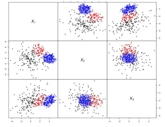
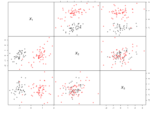
For all three families, the BIC selects a three-component model for each of the 100 runs. For the ePEM family, the BIC selects an EEEV (VVEE) model 99 (1) times. The ARI values for the selected models from the mixture family range between 0.87 and 0.96 with a median (mean) value of 0.92 (0.92). Similarly, the teigen family yields ARI values between 0.85 and 0.96 with a median (mean) value of 0.92 (0.91). Even though all three families select the same number of components every time, the estimated ARI values for the selected ePEM models are higher, ranging between 0.91 and 0.98 with a median (mean) value of 0.94 (0.94). A scatter plot showing an example of the generated data is given in Figure 3. The estimated mean, covariance, and $\beta$ are given in Table 3.

Figure 3: Scatter plots showing an example of a generated data set for Simulation 2.

Table 3: True parameter values along with mean and standard deviations of the parameter estimates (rounded off to 2 decimals) for the selected model from the 100 runs for Simulation 2.

Parameter	True values	Mean estimates	Standard deviations
$\pi_{1}$	0.35	0.35	0.02
$\pi_{2}$	0.15	0.15	0.02
$\pi_{3}$	0.5	0.5	0.02
$\mbox{\boldmath$\mu$}_{1}$	$(0,2,0)^{\prime}$	$(-0.02,1.97,0.01)^{\prime}$	$(0.12,0.18,0.14)^{\prime}$
$\mbox{\boldmath$\mu$}_{2}$	$(2,5,0)^{\prime}$	$(1.99,4.98,0.00)^{\prime}$	$(0.08,0.12,0.10)^{\prime}$
$\mbox{\boldmath$\mu$}_{3}$	$(4,2,0)^{\prime}$	$(4.00,2.00,0.01)^{\prime}$	$(0.03,0.04,0.03)^{\prime}$
$\text{Covariance}_{1}$	$\begin{pmatrix}2.86&-0.45&1.75\\ -0.45&5.64&-0.59\\ 1.75&-0.59&3.89\\ \end{pmatrix}$	$\begin{pmatrix}2.88&-0.41&1.75\\ -0.41&5.71&-0.57\\ 1.75&-0.57&3.89\\ \end{pmatrix}$	$\begin{pmatrix}0.27&0.16&0.20\\ 0.16&0.53&0.18\\ 0.20&0.18&0.34\\ \end{pmatrix}$
$\text{Covariance}_{2}$	$\begin{pmatrix}0.49&-0.08&0.30\\ -0.08&0.97&-0.10\\ 0.30&-0.10&0.67\\ \end{pmatrix}$	$\begin{pmatrix}0.49&-0.07&0.30\\ -0.07&0.98&-0.10\\ 0.30&-0.10&0.67\\ \end{pmatrix}$	$\begin{pmatrix}0.05&0.03&0.04\\ 0.03&0.09&0.03\\ 0.04&0.03&0.06\\ \end{pmatrix}$
$\text{Covariance}_{3}$	$\begin{pmatrix}0.42&-0.07&0.26\\ -0.07&0.83&-0.09\\ 0.26&-0.09&0.57\\ \end{pmatrix}$	$\begin{pmatrix}0.42&-0.06&0.25\\ -0.06&0.83&-0.08\\ 0.25&-0.08&0.57\\ \end{pmatrix}$	$\begin{pmatrix}0.02&0.02&0.02\\ 0.02&0.04&0.02\\ 0.02&0.02&0.03\\ \end{pmatrix}$
$\beta_{1}$	0.85	0.87	0.17
$\beta_{2}$	3	3.49	1.22
$\beta_{3}$	5	5.93	1.37

Simulation 3: Higher-dimensional data

Here, parameter recovery is illustrated for the ePEM family on higher dimensional data. One-hundred samples of a thirty dimensional two-component mixture model are simulated in the fashion of Murray et al. (2014). Group sample sizes are sampled from a binomial distribution with success probability $0.35$ and an overall sample size of 400. The first component is simulated from a 30-dimensional MPE distribution with zero mean. The second component is simulated from a 30-dimensional MPE distribution with mean $(3,3,3)^{\prime}\otimes\boldsymbol{1}_{10}$, where $\boldsymbol{1}_{10}$ denotes a column vector of length 10 with all entries equalling 1. The common scale matrix is generated using

$$\begin{pmatrix}1&0.1&0.2\\ 0.1&1.5&0.3\\ 0.2&0.3&1.2\end{pmatrix}\otimes\boldsymbol{I}_{10},$$

where $\boldsymbol{I}_{10}$ denotes a 10-dimensional identity diagonal matrix. The recovered parameter estimates are found to be close on average to the generating parameters. Due to the dimensionality, we follow Murray et al. (2014) and report the Frobenius norms of the biases of the parameter estimates in Table 4. Clearly, the estimated parameters are quite close to the generating parameters. Note that while the purpose of this simulation is to investigate parameter estimation in higher dimensions, all 100 runs yield perfect clustering.

Table 4: True parameter values along with the Frobenius norms of the biases of the parameter estimates (rounded off to 2 decimals) for the selected model from the 100 runs for Simulation 3.

Parameter	True values	$\|\text{Bias}\|$
$\pi_{1}$	0.35	0.00
$\pi_{2}$	0.65	0.00
$\mbox{\boldmath$\mu$}_{1}$	$(0,0,0)^{\prime}\otimes\boldsymbol{1}_{10}$	0.02
$\mbox{\boldmath$\mu$}_{2}$	$(3,3,3)^{\prime}\otimes\boldsymbol{1}_{10}$	0.05
$\text{Covariance}_{1}$	$\frac{2^{1/\beta_{1}}\Gamma\left(\frac{p+2}{2\beta_{1}}\right)}{p\Gamma\left(\frac{p}{2\beta_{1}}\right)}\times\begin{pmatrix}1&0.1&0.2\\ 0.1&1.5&0.3\\ 0.2&0.3&1.2\end{pmatrix}\otimes\boldsymbol{I}_{10}$	0.26
$\text{Covariance}_{2}$	$\frac{2^{1/\beta_{2}}\Gamma\left(\frac{p+2}{2\beta_{2}}\right)}{p\Gamma\left(\frac{p}{2\beta_{2}}\right)}\times\begin{pmatrix}1&0.1&0.2\\ 0.1&1.5&0.3\\ 0.2&0.3&1.2\end{pmatrix}\otimes\boldsymbol{I}_{10}$	2.55
$\beta_{1}$	2	0.34
$\beta_{2}$	0.95	0.08

Simulation 4: Gaussian and $t$-components

Here, we show that the ePEM family can recover Gaussian and $t$-components favourably when compared to the mixture and teigen families. A two-component mixture is simulated with 100 observations, where the group sample sizes are sampled from a binomial distribution with success probability $0.4$. The first component is simulated from a 3-dimensional Gaussian distribution with zero mean. The second component is simulated from a 3-dimensional $t$-distribution with mean $(5,0,0)^{\prime}$ and 5 degrees of freedom. Both components are generated using the same scale matrix:

$$\begin{pmatrix}1&0.5&0.25\\ 0.5&1&0.3\\ 0.25&0.3&1\end{pmatrix}.$$

The algorithms are run for $G=1,\ldots,5$. The mixture family does not perform well over 100 runs. One through five component models are chosen 1, 52, 31, 14, and 2 times, respectively. In contrast, for the ePEM family, a two (three) component model is selected 89 (11) times. On the occasion when a three-component model is selected, the low overall sample size seems to contribute to some observations from the heavy-tailed component being clustered in their own unique group. Similarly, for the teigen family, a two (three) component model is selected 88 (12) times. Over the 100 runs, the EEEE (EEEV) model is selected 70 (21) times. Given the generated data, a model with varying $\beta_{g}$ might be expected from the ePEM family; however, in a few runs, the selected models have heavy tailed components with equal $\beta_{g}$. This may be due to the small overall sample size and/or the fact that the generated components are not clearly separated. The ARI values for the selected models for the mixture family over the 100 runs range from 0 (for the one-component model) to 1, with a median (mean) ARI of 0.94 (0.90). Similarly, the selected models from both the teigen and ePEM families yield ARI values ranging between 0.57 and 1, with a median (mean) value of 0.96 (0.94). A scatter plot showing an example of the generated data is given in Figure 4.

Figure 4: Scatter plots showing an example of a generated data set for Simulation 3.

Assessing the impact of outliers

We follow McLachlan and Peel (2000b) in assessing the impact of outliers on the clustering performance of the ePEM family as compared to the Gaussian mixture models implemented in the mixture package. The crab data set, introduced in Campbell and Mahon (1974), consists of five-dimensional observations on crabs of the genus Leptograpsus and can be obtained from the MASS package (Venables and Ripley, 2002). Measurements are recorded on the width of the front lip, the rear width, the length along the middle, the maximum width of the carapace, and the body depth. The subset of blue crabs (50 males and 50 females) is analyzed in McLachlan and Peel (2000b), where outliers are introduced, and a Gaussian model with a common covariance matrix as well as a $t$-mixture model with equal scale matrices and equal degrees of freedom are fitted. The outliers are introduced by adding various values to the second variate of the $25^{\text{th}}$ point. We replicate this analysis to investigate the performance of the ePEM models compared to the mixture models. Note that the EEEE model from the teigen family is also fitted but does not perform well (a minimum of 37 misclassifications; results not shown). This is probably due to different starting values; however, McLachlan and Peel (2000b) do not provide information on the starting values used for their comparison and we are unable to obtain results similar to theirs. On the original data, Gaussian EEE and MPE EEEE two-component models yield 19 misclassifications each. However, as the value of the constant that is added to the observation of interest is increased or decreased, the MPE component model error rate is much smaller than that of the Gaussian mixture. However, both the Gaussian mixture and MPE approach suffer when the constant by which the value is jittered is extreme.

Table 5: Comparison of error rates from the Gaussian and MPE mixture models fitted to modified crabs data.

Constant	Gaussian	MPE	$\hat{\beta}$
$-15$	37	35	0.43
$-10$	40	21	0.46
$-5$	42	20	0.73
$0$	19	19	0.80
$5$	22	20	0.67
$10$	36	37	0.52
$15$	38	41	0.43

Entries in the first column are the values added to the second variate of the $25^{\text{th}}$ observation to make it an outlier. Entries in the second and third columns are the number of misclassifications for the Gaussian and MPE mixture models, respectively. Lastly, the $\hat{\beta}$ values are also provided.

4.2 Real Data

We also test our algorithm’s performance on several real benchmark data sets. The body, diabetes, female voles, and wine data sets are commonly used for illustration in the model-based clustering literature. We also consider two bioinformatics data sets: the srbct data and the glob data. The body data contain 24 measurements on body dimension, age, weight, and height for 507 individuals (247 men and 260 women), and can be obtained from the gclus package (Hurley, 2012). The diabetes data (Reaven and Miller, 1979), obtained from mclust, contains three measurements on 145 subjects from three classes: chemical (36 observations), normal (76 observations), and overt (33 observations). The female voles data (Airoldi and Hoffmann, 1984) contain seven measurements on age and skull size of 86 females of two species of voles: Microtus californicus (41 observations) and M. Ochrogaster (45 observations). These data are available as part of the Flury package (Flury, 2012) in R. Lastly, the wine data (Forina et al., 1988) contain 13 measurements on 178 wines of three types (barolo, grignolino, and barbera), and can be obtained from the gclus package.

The srbct data contain gene expression microarray data from experiments on small round blue cell tumors (Khan et al., 2001). A preprocessed version of these data can be obtained from the plsgenomics package (Boulesteix et al., 2014). The 83 samples are known to correspond to four classes, including 29 cases of Ewing sarcoma, 11 cases of Burkitt lymphoma, 18 cases of neuroblastoma, and 25 cases of rhabdomyosarcoma. The golub data contain gene expression data from Golub et al. (1999) on two forms of acute leukaemia: acute lymphoblastic leukaemia (47 observations) and acute myeloid leukaemia (25 observations). The preprocessed data used in the analysis of McNicholas and Murphy (2010) are available at www.paulmcnicholas.info. Note that methodology proposed herein is not designed for high-dimensional, low sample size (i.e., large $p$, small $N$) problems — the development of factor analysis-based extensions of MPE mixture models, along the lines of the mixture of factor analyzers model (Ghahramani and Hinton, 1997; McLachlan and Peel, 2000a) and extensions thereof (e.g., McNicholas and Murphy, 2008; Andrews and McNicholas, 2011), will be a subject of future work. Hence, both of these bioinformatics data sets are further pre-processed to make the clustering problem more suitable for the methodology that is the subject of the present work. A differential expression analysis on the gene expression data is performed using an ANOVA across the known groups. The top ten genes, ranked using the obtained p-values, are selected to represent a potential set of measurements that contain information allowing for identification of the four groups. The three mixture model-based clustering algorithms were then run on these processed data. The ePEM family is run on the scaled data for $G=1,\ldots,5$. Table 6 compares the performance of the methodologies run on these data; here, the predicted classifications from the selected model (using the BIC) are compared to the true class labels in each case.

Table 6: Comparison of three families of mixture models on benchmark data.

Data	ePEM	mixture	teigen
body ($p=24$, $G=2$)	0.94 (2; EEEV)	0.80 (3; EEE)	0.80 (3; EEEE)
diabetes ($p=3$, $G=3$)	0.66 (3; VVVE)	0.66 (3; VVV)	0.67 (3; VVVE)
female voles ($p=7$, $G=2$)	0.91 (2; EEEV)	0.91 (2; EEE)	0.91 (2; EEEE)
wine ($p=13$, $G=3$)	0.98 (3; EEEV)	0.68 (4; VVI)	0.68 (4; VVIE)
srbct ($p=10$, $G=4$)	0.82 (4; VIIE)	0.82 (4; VVI)	0.85 (4; VVIE)
golub ($p=10$, $G=2$)	0.84 (2; EEIE)	0.47 (5; VVE)	0.74 (2; VVIE)

Dimensionality and the number of known groups (i.e., classes) are in parenthesis following the name of each data set. For each family of models, the ARI, the number of components, and scale structure for the selected model are given in parenthesis.

Clearly, the ePEM family performs favourably compared to the mixture and teigen families. For the body data, the selected ePEM model fits a mixture of two heavy tailed components, i.e., $\hat{\mbox{\boldmath$\beta$}}=(0.57,0.56)^{\prime}$, that misclassifies eight cases (4 of each gender). The teigen family selects a model with 3 heavy-tailed components (23.43 degrees of freedom each), and the selected mixture model also fits three components. For the diabetes data, the selected models from all three families yield similar classifications, each with a total of 20 misclassifications. The selected ePEM model has $\hat{\beta}=1.07$ in each component, suggesting components that are close to Gaussian. The selected teigen model also has relatively high (50.30) degrees of freedom in each component, implying component shapes that are close to Gaussian. For the female voles data, the selected models from all three families yield the same classification results, each with two misclassifications. For the wine data, both the selected mixture and teigen models have four components, with 19.15 degrees of freedom in each component for the chosen teigen model. However, the selected ePEM model has three components, with $\hat{\mbox{\boldmath$\beta$}}=(0.62,0.59,0.56)^{\prime}$, and misclassifies only one observation, whereas the selected mixture and teigen models misclassify 35 and 34 observations, respectively.

For the srbct data, the selected teigen model performs slightly better than the selected mixture and ePEM models. All selected models fit four components with the selected teigen, mixture, and ePEM models misclassifying 4, 5, and 5 observations, respectively. The selected teigen model has 15.53 degrees of freedom in each component, while the selected ePEM model has $\hat{\beta}=0.42$ in each component.

Despite similar outcomes being obtained for the srbct data, the results differ greatly for the golub data. The selected mixture and teigen models have five and two components, respectively. A referee asked us to comment on situations where the number of parameters approaches the number of observations. A restriction can be imposed such that only those models are fitted that estimate fewer parameters than the number of observations in the sample. The selected five-component mixture model has more parameters than there are observations. Restricting mixture to only those models with fewer parameters than the number of observations, a three-component model is selected with an ARI value of 0.76. The selected ePEM model also has two components with $\hat{\beta}=0.28$ in each component, and yields a higher ARI than the selected teigen model, which has 5.80 degrees of freedom in each component.

Overall, on these real data sets, the ePEM family outperforms the corresponding family of Gaussian mixtures and performs at least as well as the corresponding mixtures of $t$-distributions. Note that the BIC and the ICL picked the same ePEM model for all real data sets. We also ran these three algorithms on other commonly used data in model-based clustering: the Swiss bank note (Flury, 2012) and the iris (Anderson, 1935; Fisher, 1936) data sets. On these data, the selected models from all three algorithms fit the same number of components and had approximately the same ARI values (results not shown).

5 Discussion

A family of MPE mixture models was proposed based on the density introduced in Gómez et al. (1998). This expanded family of mixture models is introduced with a greatly improved parameter estimation procedure as compared to the techniques proposed previously. This family of mixture models is unique in being able to deal with both lighter and heavier tails than the Gaussian distribution. Mixtures of $t$-distributions can only account for heavier than Gaussian tails and suffers when fitted to lighter tailed data. In such cases, both mixtures of $t$-distributions and mixtures of Gaussian distributions often fit more than the true number of components. Using simulations, we showed that the ePEM family is a good alternative to mixtures of Gaussian and mixtures of Student-$t$ distributions, and that it is able to handle Gaussian, heavy-tailed, and light-tailed components. Moreover, these models also allow for different levels of peakedness of data: from thin to Gaussian to flat. Hence, these models are also well suited for density estimation purposes for a wide range of non-Gaussian data.

Estimation is provided for eight scale structures that can be obtained through the use of eigen-decomposition of the scale matrix. Previously, mixtures of Gaussian and uniform distributions have been fitted to account for outliers (Banfield and Raftery, 1993; Hennig and Coretto, 2008; Coretto and Hennig, 2010). In our framework, a uniform component can be conveniently approximated by restricting $\beta$ to be high because the power exponential distribution becomes a multivariate generalization of the uniform distribution. This enables greater parsimony than a mixture of Gaussian and uniform distributions when fitted to data with random noise, e.g., on mean-centred data, an EIIE model requires estimation of only one additional parameter. A mixture of skewed power exponential distributions will be a focus of future work; such a model will be better suited to modelling data with asymmetric clusters. Lastly, note that the ePEM family has heavy fat tails for higher dimensions (Liu and Bozdogan, 2008); therefore, a mixture of power exponential factor analyzers model may be useful for higher-dimensional data with outliers.

Appendix

Appendix A Fixed-point algorithm

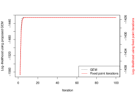
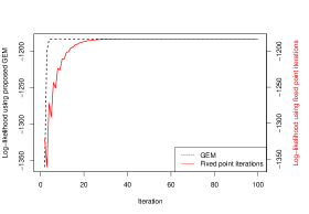
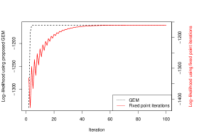
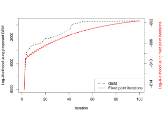
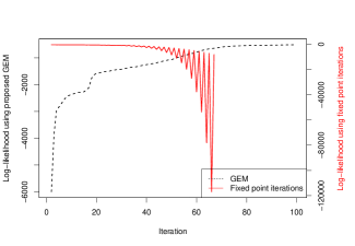
Zhang and Liang (2010) used fixed point iterative estimates for $\mbox{\boldmath$\Sigma$}_{g}$. Note that the MPE density used in Zhang and Liang (2010) can be obtained by setting $\mbox{\boldmath$\Sigma$}=2\mbox{\boldmath$\Delta$}$, $r=2^{\beta^{*}}$, and $s=\beta^{*}/2$ in (1), where $\Delta$ denotes the scale matrix in the parameterization of Zhang and Liang (2010). We show that the estimation procedure used in Zhang and Liang (2010) is valid only for $\beta^{*}\in(0,4)$, where $\beta^{*}$ is defined as in Zhang and Liang (2010). A proof for this (see Appendix A.1) applies to $\beta\in(0,2]$, because of the different shape parameterizations, without loss of generality. In Figure 5, we present four comparisons of the trajectory of log-likelihood values between our proposed estimation and using fixed point iterations: for $\beta$ equaling 1.5, 1.9, 1.95, and 2.05, respectively. For all cases, 1000 observations were generated from a 2-dimensional zero-centred power exponential distribution. Only $\Sigma$ is estimated, with the other parameters held constant. For both algorithms, $\Sigma$ is initialized as an identity matrix. Clearly, as $\beta$ approaches 2, the log-likelihood values for the fixed point estimating procedure (red line) oscillate more heavily. This leads to non-monotonicity of the likelihood, complicating the determination of convergence. Moreover, notice that certain values of the log-likelihood for the fixed point are not plotted for $\beta=2.05$—this is because of numerical errors. Note that each of the subplots in Figure 5 has two ordinate axes due to different scales of the values from each procedure. We also provide similar plots for $\beta$ equaling 1.99 and 2.05 for a 10-dimensional simulation (Figure 6). The results are quite similar. We have conducted extensive simulations and, in every case, the log-likelihood values from the fixed point iterations diverge for $\beta>2$. In most cases, the fixed point iterations do not even run. Because this is equivalent to $\beta^{*}>4$, we conclude that the GEM approach is better than using fixed point iterations. Furthermore, note that for $\beta^{*}<2$, the fixed point algorithm for an unconstrained scale matrix converges due to concavity properties (similar to our VVV case for $0<\beta<1$). Note that Zhang and Liang (2010) only deal with $\beta^{*}\leq 4$ in their work.

Figure 5: Log-likelihood plots for our GEM procedure and fixed point-based estimating algorithms for two-dimensional data. The top-left, top-right, bottom-left and bottom-right panel have $\beta$ equaling 1.5, 1.9, 1.95, and 2.05, respectively.

Figure 6: Log-likelihood plots for the proposed GEM procedure and fixed point-based estimating algorithms on 10-dimensional data. The left- and right-hand panels have $\beta$ values of 1.99 and 2.05, respectively.

A.1 Fixed point stability

The fixed point algorithm from Zhang and Liang (2010) diverges for $\beta>2$

Proof.

If $\boldsymbol{X}$ follows a $p$-dimensional power exponential distribution, the log-likelihood with respect to $\Sigma$ is

$$\mathcal{L}(\mbox{\boldmath$\Sigma$})=\sum_{i=1}^{N}\sum_{g=1}^{G}\frac{1}{2}\log|{\mbox{\boldmath$\Sigma$}}|^{-1}-\frac{1}{2}\left[(\boldsymbol{x}_{i}-\mbox{\boldmath$\mu$})^{\prime}\mbox{\boldmath$\Sigma$}^{-1}(\boldsymbol{x}_{i}-\mbox{\boldmath$\mu$})\right]^{\beta}.$$

Then, upon taking the derivative of $\mathcal{L}(\mbox{\boldmath$\Sigma$})$ with respect to $\mbox{\boldmath$\Sigma$}^{-1}$, we can obtain the fixed point update

$$f(\mbox{\boldmath$\Sigma$})=\frac{\beta}{N}\sum_{i=1}^{N}\left[(\boldsymbol{x}_{i}-\mbox{\boldmath$\mu$})^{\prime}\mbox{\boldmath$\Sigma$}^{-1}(\boldsymbol{x}_{i}-\mbox{\boldmath$\mu$})\right]^{\beta-1}(\boldsymbol{x}_{i}-\mbox{\boldmath$\mu$})(\boldsymbol{x}_{i}-\mbox{\boldmath$\mu$})^{\prime}.$$ (5)

Now,

$$\operatorname{vec}(f(\mbox{\boldmath$\Sigma$}))=\frac{\beta}{N}\sum_{i=1}^{N}\left[(\boldsymbol{x}_{i}-\mbox{\boldmath$\mu$})^{\prime}\mbox{\boldmath$\Sigma$}^{-1}(\boldsymbol{x}_{i}-\mbox{\boldmath$\mu$})\right]^{\beta-1}\operatorname{vec}((\boldsymbol{x}_{i}-\mbox{\boldmath$\mu$})\otimes(\boldsymbol{x}_{i}-\mbox{\boldmath$\mu$})).$$

Taking the derivative with respect to $\Sigma$, we get the Jacobian

$$\boldsymbol{J} =\frac{\beta(1-\beta)}{N}\sum_{i=1}^{N}\left[(\boldsymbol{x}_{i}-\mbox{\boldmath$\mu$})^{\prime}\mbox{\boldmath$\Sigma$}^{-1}(\boldsymbol{x}_{i}-\mbox{\boldmath$\mu$})\right]^{\beta-2}$$

$$\qquad\qquad\qquad\qquad\times\operatorname{vec}((\boldsymbol{x}_{i}-\mbox{\boldmath$\mu$})\otimes(\boldsymbol{x}_{i}-\mbox{\boldmath$\mu$}))\operatorname{vec}(\mbox{\boldmath$\Sigma$}^{-1}(\boldsymbol{x}_{i}-\mbox{\boldmath$\mu$})(\boldsymbol{x}_{i}-\mbox{\boldmath$\mu$})^{\prime}\mbox{\boldmath$\Sigma$}^{-1})^{\prime}$$

$$=\frac{\beta(1-\beta)}{N}\sum_{i=1}^{N}\left\{\left[(\boldsymbol{x}_{i}-\mbox{\boldmath$\mu$})^{\prime}\mbox{\boldmath$\Sigma$}^{-1}(\boldsymbol{x}_{i}-\mbox{\boldmath$\mu$})\right]^{\beta-2}\right.$$

$$\qquad\qquad\qquad\qquad\times\left.\operatorname{vec}((\boldsymbol{x}_{i}-\mbox{\boldmath$\mu$})\otimes(\boldsymbol{x}_{i}-\mbox{\boldmath$\mu$}))\left[\operatorname{vec}(\mbox{\boldmath$\Sigma$}^{-1}\otimes\mbox{\boldmath$\Sigma$}^{-1})\operatorname{vec}((\boldsymbol{x}_{i}-\mbox{\boldmath$\mu$})\otimes(\boldsymbol{x}_{i}-\mbox{\boldmath$\mu$}))\right]^{\prime}\right\}.$$

Then,

$$\operatorname{tr}(\boldsymbol{J}) =\frac{\beta(1-\beta)}{N}\sum_{i=1}^{N}\left[(\boldsymbol{x}_{i}-\mbox{\boldmath$\mu$})^{\prime}\mbox{\boldmath$\Sigma$}^{-1}(\boldsymbol{x}_{i}-\mbox{\boldmath$\mu$})\right]^{\beta-2}$$

$$\qquad\qquad\qquad\qquad\qquad\times\operatorname{tr}\left\{(\boldsymbol{x}_{i}-\mbox{\boldmath$\mu$})(\boldsymbol{x}_{i}-\mbox{\boldmath$\mu$})^{\prime}\mbox{\boldmath$\Sigma$}^{-1}\otimes(\boldsymbol{x}_{i}-\mbox{\boldmath$\mu$})(\boldsymbol{x}_{i}-\mbox{\boldmath$\mu$})^{\prime}\mbox{\boldmath$\Sigma$}^{-1}\right\}$$

$$=\frac{\beta(1-\beta)}{N}\sum_{i=1}^{N}\left[(\boldsymbol{x}_{i}-\mbox{\boldmath$\mu$})^{\prime}\mbox{\boldmath$\Sigma$}^{-1}(\boldsymbol{x}_{i}-\mbox{\boldmath$\mu$})\right]^{\beta-2}$$

$$\qquad\qquad\qquad\qquad\qquad\times\operatorname{tr}\left\{(\boldsymbol{x}_{i}-\mbox{\boldmath$\mu$})(\boldsymbol{x}_{i}-\mbox{\boldmath$\mu$})^{\prime}\mbox{\boldmath$\Sigma$}^{-1}\right\}\operatorname{tr}\left\{(\boldsymbol{x}_{i}-\mbox{\boldmath$\mu$})(\boldsymbol{x}_{i}-\mbox{\boldmath$\mu$})^{\prime}\mbox{\boldmath$\Sigma$}^{-1}\right\}$$

$$=\operatorname{tr}\left\{(1-\beta)\mbox{\boldmath$\Sigma$}^{-1}\frac{\beta}{N}\sum_{i=1}^{N}\left[(\boldsymbol{x}_{i}-\mbox{\boldmath$\mu$})^{\prime}\mbox{\boldmath$\Sigma$}^{-1}(\boldsymbol{x}_{i}-\mbox{\boldmath$\mu$})\right]^{\beta-1}(\boldsymbol{x}_{i}-\mbox{\boldmath$\mu$})(\boldsymbol{x}_{i}-\mbox{\boldmath$\mu$})^{\prime}\right\}.$$

Evaluating $\operatorname{tr}(\boldsymbol{J})$ at $\mbox{\boldmath$\Sigma$}=\hat{\mbox{\boldmath$\Sigma$}}$, we get $\operatorname{tr}(\boldsymbol{I}_{p}(1-\beta))=(1-\beta)p$. Now, because the matrix norm $||\boldsymbol{B}||_{p}=\operatorname{tr}(\boldsymbol{B}^{p})^{1/p}$, $||\boldsymbol{J}||_{1}=\operatorname{tr}(\boldsymbol{J})=p(1-\beta)$. Also, note that because $||J||_{1}\leq p||J||_{\infty}$, and we require $||J||_{\infty}<1$ for stability ($||J||_{\infty}=1$ for neutrality), we have

$$||J||_{1}\leq p||J||_{\infty}<p.$$

Hence, $p(1-\beta)<p$, leading to $0<\beta<2$. Therefore, the solution diverges for $\beta>2$. ∎

Appendix B Inference

The likelihood of the MPE mixture model is

$$L_{0}(\mbox{\boldmath$\Theta$}|\mathcal{S})=\prod_{i=1}^{N}\sum_{g=1}^{G}\pi_{g}k_{g}|\mbox{\boldmath$\Sigma$}_{g}|^{-\frac{1}{2}}\exp\left\{-\frac{1}{2}\left((\boldsymbol{x}_{i}-\boldsymbol{\mu})_{ig}^{\prime}\mbox{\boldmath$\Sigma$}_{g}^{-1}(\boldsymbol{x}_{i}-\boldsymbol{\mu})_{ig}\right)^{\beta_{g}}\right\},$$

where $k_{g}$ is analogous to $k$ in (2), and $(\boldsymbol{x}_{i}-\boldsymbol{\mu})_{ig}=\boldsymbol{x}_{i}-\mbox{\boldmath$\mu$}_{g}$. Note that $\mathcal{S}$ is considered incomplete in the context of the EM algorithm. The complete-data are $\mathcal{S}_{\text{c}}=\left\{(\boldsymbol{x}_{1},\boldsymbol{z}_{1}),\ldots,(\boldsymbol{x}_{N},\boldsymbol{z}_{N})\right\}$, where the missing data $\boldsymbol{z}_{i}=(z_{i1},\ldots,z_{iG})^{\prime}$ is the component label vector such that $z_{ig}$ = 1 if $\boldsymbol{x}_{i}$ comes from the $g^{\text{th}}$ population and 0 otherwise. The complete-data log-likelihood $\mathcal{L}_{c}(\mbox{\boldmath$\Theta$})=\log{L_{c}(\mbox{\boldmath$\Theta$}|\mathcal{S}_{\text{c}})}$ can be written as

$$\mathcal{L}_{c}(\mbox{\boldmath$\Theta$})=\sum_{i=1}^{N}\sum_{g=1}^{G}z_{ig}\log\left[\pi_{g}k_{g}|\mbox{\boldmath$\Sigma$}_{g}|^{-\frac{1}{2}}\exp\left\{-\frac{\delta_{ig}(\boldsymbol{x}_{i})^{\beta_{g}}}{2}\right\}\right].$$

where $\delta_{ig}(\boldsymbol{x}_{i}):=\delta_{i}\left(\boldsymbol{x}_{i}|\mbox{\boldmath$\mu$}_{g},\mbox{\boldmath$\Sigma$}_{g}\right)=\left(\boldsymbol{x}_{i}-\mbox{\boldmath$\mu$}_{g}\right)^{\prime}\mbox{\boldmath$\Sigma$}_{g}^{-1}\left(\boldsymbol{x}_{g}-\mbox{\boldmath$\mu$}_{g}\right)$. The E-step involves calculating the expected complete-data log-likelihood, which we denote $\mathcal{Q}$. We need the expected values

$$\tau_{ig}\colonequals\mathbb{E}_{\widehat{}\mbox{\boldmath$\Theta$}}[Z_{ig}|\boldsymbol{x}_{i}]=\frac{\pi_{g}f\left(\boldsymbol{x}_{i}|\hat{}\mbox{\boldmath$\mu$}_{g},\hat{}\mbox{\boldmath$\Sigma$}_{g},\hat{\beta}_{g}\right)}{\sum_{j=1}^{G}\hat{\pi}_{j}f\left(\boldsymbol{x}_{i}|\hat{}\mbox{\boldmath$\mu$}_{j},\hat{}\mbox{\boldmath$\Sigma$}_{j},\hat{\beta}_{j}\right)},$$ (6)

for $i=1,\ldots,N$ and $g=1,\ldots,G$. The M-step on the $(k+1)$th iteration involves maximization of the expected value of the complete-data log-likelihood with respect to $\Theta$. The update for $\hat{\pi}_{g}$ is

$$\hat{\pi}_{g}={n_{g}}/{N},$$

where $n_{g}=\sum_{i=1}^{N}\tau_{ig}$.

However, the updates for $\hat{\beta}_{g}$, $\hat{\mbox{\boldmath$\mu$}}_{g}$, and $\hat{\mbox{\boldmath$\Sigma$}}_{g}$ are not available in closed form. A Newton-Raphson update is used to find the update for $\hat{\mbox{\boldmath$\mu$}}_{g}$, and we need the following:

$$\frac{\partial\mathcal{Q}}{\partial\mbox{\boldmath$\mu$}_{g}}= \hat{\beta}_{g}\sum_{i=1}^{N}\tau_{ig}\delta_{ig}(\boldsymbol{x}_{i})^{\hat{\beta}_{g}-1}\hat{\mbox{\boldmath$\Sigma$}}_{g}^{-1}(\boldsymbol{x}_{i}-\boldsymbol{\mu})_{ig}$$ (7)

$$\frac{\partial^{2}\mathcal{Q}}{\partial\mbox{\boldmath$\mu$}_{g}\mbox{\boldmath$\mu$}_{g}^{\prime}}= \hat{\beta}_{g}\sum_{i=1}^{N}\tau_{ig}\left[-\delta_{ig}(\boldsymbol{x}_{i})^{\hat{\beta}_{g}-1}\hat{\mbox{\boldmath$\Sigma$}}_{g}^{-1}+(\hat{\beta}_{g}-1)\delta_{ig}(\boldsymbol{x}_{i})^{\hat{\beta}_{g}-2}\hat{\mbox{\boldmath$\Sigma$}}_{g}^{-1}(\boldsymbol{x}_{i}-\boldsymbol{\mu})_{ig}\big{(}-2\hat{\mbox{\boldmath$\Sigma$}}_{g}^{-1}(\boldsymbol{x}_{i}-\boldsymbol{\mu})_{ig}\big{)}^{\prime}\right],$$ (8)

where $\delta_{ig}(\boldsymbol{x}_{i}):=\left(\boldsymbol{x}_{i}-\hat{\mbox{\boldmath$\mu$}}_{g}\right)^{\prime}\hat{\mbox{\boldmath$\Sigma$}}_{g}^{-1}\left(\boldsymbol{x}_{i}-\hat{\mbox{\boldmath$\mu$}}_{g}\right)$ and $(\boldsymbol{x}_{i}-\boldsymbol{\mu})_{ig}=\boldsymbol{x}_{i}-\hat{\mbox{\boldmath$\mu$}}_{g}$. An update for $\hat{\beta}_{g}$ can be obtained by solving the equation

$$\frac{pn_{g}}{\left(\hat{\beta}_{g}^{\mbox{\tiny new}}\right)^{2}} \psi\left(1+\frac{p}{2\hat{\beta}_{g}^{\mbox{\tiny new}}}\right)+\frac{pn_{g}\log 2}{\left(\hat{\beta}_{g}^{\mbox{\tiny new}}\right)^{2}}-\sum_{i=1}^{N}\tau_{ig}[\log{\delta_{ig}(\boldsymbol{x}_{i})}]\left(\delta_{ig}(\boldsymbol{x}_{i})\right)^{\hat{\beta}_{g}^{\mbox{\tiny new}}}=0$$ (9)

for $\hat{\beta}_{g}^{\mbox{\tiny new}}$, where $\psi(\cdot)$ is the digamma function. Alternatively, a Newton-Raphson method might be implemented using the following:

$$\frac{\partial\mathcal{Q}}{\partial\beta_{g}}= \frac{pn_{g}}{2\hat{\beta}_{g}^{2}}\psi\left(1+\frac{p}{2\hat{\beta}_{g}}\right)+\frac{pn_{g}\log{2}}{2\hat{\beta}_{g}^{2}}-\sum_{i=1}^{N}\frac{\tau_{ig}}{2}\delta_{ig}(\boldsymbol{x}_{i})^{\hat{\beta}_{g}}\log{\delta_{ig}(\boldsymbol{x}_{i})}$$ (10)

$$\frac{\partial^{2}\mathcal{Q}}{\partial\beta_{g}^{2}}= \frac{-pn_{g}}{\hat{\beta}_{g}^{3}}\psi\left(1+\frac{p}{2\hat{\beta}_{g}}\right)-\frac{p^{2}n_{g}}{4\hat{\beta}_{g}^{4}}\psi_{1}\left(1+\frac{p}{2\hat{\beta}_{g}}\right)-\frac{pn_{g}\log{2}}{\hat{\beta}_{g}^{3}}-\sum_{i=1}^{N}\frac{\tau_{ig}}{2}\delta_{ig}(\boldsymbol{x}_{i})^{\hat{\beta}_{g}}\left[\log{\delta_{ig}(\boldsymbol{x}_{i})}\right]^{2},$$ (11)

where $\psi_{1}(\cdot)$ is the trigamma function. Uptates for $\hat{\beta}_{g}$ when it is constrained to be equal between groups can be obtained similarly. Because the update for $\hat{}\mbox{\boldmath$\Sigma$}_{g}$ is not available in closed form, we rely on convexity properties. For the updates for the EEI, VVI, EEE, EEV, VVE, and VVV scale matrices, we utilize a minorization-maximization step. Because of the properties of a minorization-maximization algorithm, this step increases the expected value of the complete-data log-likelihood at every iteration, thus making the estimation algorithm a generalized EM (GEM) algorithm. In addition, for the EEE, EEV, VVE, and VVV scale matrices, we utilize an accelerated line search method on the orthogonal Stiefel manifold (cf. Absil et al., 2009; Browne and McNicholas, 2014b). An MM algorithm can be constructed by using the convexity of the objective function—a surrogate minorizing function is employed that is maximized. Note that the surrogate function constructed in the E-step in an EM algorithm is, up to a constant, a minorizing function (Hunter and Lange, 2004). For the EII, VII, EEI, VVI, EEE, EEV, VVE, and VVV scale structures (as listed in Table 1), the updates are discussed below. The pseudo-code for the estimation of parameters is:

1. Initialize $\hat{\beta}_{g}$, $\hat{}\mbox{\boldmath$\mu$}_{g}$, $\hat{}\mbox{\boldmath$\Sigma$}_{g}$. Compute (6).

2. Update $\hat{\beta}_{g}$ using either (9) or (10) and (11); or (12) or (13) and (14), depending on whether $\beta_{g}$ is unconstrained between groups or not.

3. CM step 1: Update $\hat{}\mbox{\boldmath$\mu$}_{g}$ using (7) and (8).

4. CM step 2: Update $\hat{}\mbox{\boldmath$\Sigma$}_{g}$ depending on the scale structure.

5. Check for convergence. If not converged, go back to Step 2.

B.1 Shape parameter constrained between groups

When $\beta_{g}$ is constrained to be equal between groups, the update for $\hat{\beta}$ can be obtained by solving the equation

$$\frac{pN}{\left(\hat{\beta}^{\mbox{\tiny new}}\right)^{2}}\psi\left(1+\frac{p}{2\hat{\beta}^{\mbox{\tiny new}}}\right)+\frac{pN\log 2}{\left(\hat{\beta}^{\mbox{\tiny new}}\right)^{2}}-\sum_{g=1}^{G}\sum_{i=1}^{N}\tau_{ig}[\log{\delta_{ig}(\boldsymbol{x}_{i})}]\delta_{ig}(\boldsymbol{x}_{i})^{\hat{\beta}^{\mbox{\tiny new}}}=0$$ (12)

for $\hat{\beta}^{\mbox{\tiny new}}$. Alternatively, a Newton-Raphson method might be implemented using the following:

$$\frac{\partial\mathcal{Q}}{\partial\beta}= \frac{pN}{2\hat{\beta}^{2}}\psi\left(1+\frac{p}{2\hat{\beta}}\right)+\frac{pN\log 2}{2\hat{\beta}^{2}}-\sum_{g=1}^{G}\sum_{i=1}^{N}\frac{\tau_{ig}}{2}[\log{\delta_{ig}(\boldsymbol{x}_{i})}]\left(\delta_{ig}(\boldsymbol{x}_{i})\right)^{\hat{\beta}}$$ (13)

$$\frac{\partial^{2}\mathcal{Q}}{\partial\beta^{2}}= \frac{-pN}{\hat{\beta}^{3}}\psi\left(1+\frac{p}{2\hat{\beta}}\right)-\frac{p^{2}N}{4\hat{\beta}^{4}}\psi_{1}\left(1+\frac{p}{2\hat{\beta}}\right)-\frac{pN\log{2}}{\hat{\beta}^{3}}-\sum_{g=1}^{G}\sum_{i=1}^{N}\frac{\tau_{ig}}{2}\left[\log{\delta_{ig}(\boldsymbol{x}_{i})}\right]^{2}\delta_{ig}(\boldsymbol{x}_{i})^{\hat{\beta}}.$$ (14)

B.2 Scale structure VVV

Here, details are provided on estimation of the unconstrained scale matrix (VVV structure). On ignoring terms not involving $\mbox{\boldmath$\Sigma$}_{g}$, we have

$$\mathcal{Q}(\mbox{\boldmath$\Sigma$}_{g})=\sum_{i=1}^{N}\sum_{g=1}^{G}\frac{\tau_{ig}}{2}\log|{\mbox{\boldmath$\Sigma$}_{g}}|^{-1}-\frac{\tau_{ig}}{2}\left((\boldsymbol{x}_{i}-\boldsymbol{\mu})_{ig}^{\prime}\mbox{\boldmath$\Sigma$}_{g}^{-1}(\boldsymbol{x}_{i}-\boldsymbol{\mu})_{ig}\right)^{\beta_{g}}.$$

The updates differ based on the value of $\hat{\beta}_{g}^{\mbox{\tiny new}}$. Denote $\boldsymbol{M}_{ig}^{\mbox{\tiny new}}=(\boldsymbol{x}_{i}-\boldsymbol{\mu})_{ig}(\boldsymbol{x}_{i}-\boldsymbol{\mu})^{\prime}_{ig}$, where $(\boldsymbol{x}_{i}-\boldsymbol{\mu})_{ig}=\boldsymbol{x}_{i}-\hat{\mbox{\boldmath$\mu$}}^{\mbox{\tiny new}}_{g}$.

$\hat{\beta}_{g}^{\mbox{\tiny new}}\in(0,1)$: Here, we borrow from the minorization-maximization framework for estimation. Note that $\operatorname{tr}\left\{\mbox{\boldmath$\Sigma$}_{g}^{-1}\boldsymbol{M}_{ig}\right\}^{\beta_{g}}$ is concave for $\beta_{g}\in(0,1)$, where $\operatorname{tr}(\cdot)$ refers to the trace. A surrogate function for $\operatorname{tr}\left\{\mbox{\boldmath$\Sigma$}_{g}^{-1}\boldsymbol{M}_{ig}^{\mbox{\tiny new}}\right\}^{\beta_{g}^{\mbox{\tiny new}}}$ can be constructed using the supporting hyperplane inequality:

$$\operatorname{tr}\left\{\mbox{\boldmath$\Sigma$}_{g}^{-1}\boldsymbol{M}_{ig}^{\mbox{\tiny new}}\right\}^{\beta_{g}^{\mbox{\tiny new}}}\leq\operatorname{tr}\left\{\hat{}\mbox{\boldmath$\Sigma$}_{g}^{-1}\boldsymbol{M}_{ig}^{\mbox{\tiny new}}\right\}^{\beta_{g}^{\mbox{\tiny new}}}+ \beta_{g}^{\mbox{\tiny new}}\operatorname{tr}\left\{\hat{}\mbox{\boldmath$\Sigma$}_{g}^{-1}\boldsymbol{M}_{ig}^{\mbox{\tiny new}}\right\}^{\beta_{g}^{\mbox{\tiny new}}-1}$$

$$\times\left[\operatorname{tr}\left\{\mbox{\boldmath$\Sigma$}_{g}^{-1}\boldsymbol{M}_{ig}^{\mbox{\tiny new}}\right\}-\operatorname{tr}\left\{\hat{}\mbox{\boldmath$\Sigma$}_{g}^{-1}\boldsymbol{M}_{ig}^{\mbox{\tiny new}}\right\}\right].$$

Then, the following is maximized:

$$\sum_{i=1}^{N}\sum_{g=1}^{G} -\frac{\tau_{ig}}{2}\log|{\mbox{\boldmath$\Sigma$}_{g}}|^{-1}+\frac{\tau_{ig}}{2}\left[\operatorname{tr}\left\{\hat{}\mbox{\boldmath$\Sigma$}_{g}^{-1}\boldsymbol{M}_{ig}^{\mbox{\tiny new}}\right\}^{\hat{\beta}_{g}^{\mbox{\tiny new}}}\right.$$

$$\left.+\hat{\beta}_{g}^{\mbox{\tiny new}}\operatorname{tr}\left\{\hat{}\mbox{\boldmath$\Sigma$}_{g}^{-1}\boldsymbol{M}_{ig}^{\mbox{\tiny new}}\right\}^{\hat{\beta}_{g}^{\mbox{\tiny new}}-1}\times\left(\operatorname{tr}\left\{\mbox{\boldmath$\Sigma$}_{g}^{-1}\boldsymbol{M}_{ig}^{\mbox{\tiny new}}\right\}-\operatorname{tr}\left\{\hat{}\mbox{\boldmath$\Sigma$}_{g}^{-1}\boldsymbol{M}_{ig}^{\mbox{\tiny new}}\right\}\right)\right],$$

leading to the update

$$\hat{\mbox{\boldmath$\Sigma$}}_{g}^{\mbox{\tiny new}}=\frac{\hat{\beta}_{g}^{\mbox{\tiny new}}}{n_{g}}\sum_{i=1}^{N}\tau_{ig}\operatorname{tr}\left\{\hat{}\mbox{\boldmath$\Sigma$}_{g}^{-1}\boldsymbol{M}_{ig}^{\mbox{\tiny new}}\right\}^{\hat{\beta}_{g}^{\mbox{\tiny new}}-1}\boldsymbol{M}_{ig}^{\mbox{\tiny new}}.$$ (15)

$\hat{\beta}_{g}^{\mbox{\tiny new}}\in[1,\infty)$: Using the Jordan decomposition, $\mbox{\boldmath$\Sigma$}_{g}^{-1}=\boldsymbol{D}_{g}\boldsymbol{A}_{g}^{-1}\boldsymbol{D}_{g}^{\prime},$ where $\boldsymbol{D}_{g}$ is an orthonormal matrix and $\boldsymbol{A}_{g}$ is a diagonal matrix of eigenvalues. Now, let $\mbox{\boldmath$\Sigma$}_{g}^{-1}=\boldsymbol{D}_{g}\mbox{\boldmath$\Lambda$}_{g}^{1/\beta_{g}^{\mbox{\tiny new}}}\boldsymbol{D}_{g}^{\prime}$ where $\mbox{\boldmath$\Lambda$}_{g}^{-1/\beta_{g}^{\mbox{\tiny new}}}=\boldsymbol{A}_{g}$. We obtain updates for both $\boldsymbol{A}_{g}^{\mbox{\tiny new}}$ and $\boldsymbol{D}_{g}^{\mbox{\tiny new}}$.

It follows that

$$\operatorname{tr}\left\{(\boldsymbol{x}_{i}-\boldsymbol{\mu})^{\prime}_{ig}\hat{\boldsymbol{D}}_{g}\mbox{\boldmath$\Lambda$}_{g}^{1/\beta_{g}^{\mbox{\tiny new}}}\hat{\boldsymbol{D}}^{\prime}_{g}(\boldsymbol{x}_{i}-\boldsymbol{\mu})_{ig}\right\}^{\beta_{g}^{\mbox{\tiny new}}}=\operatorname{tr}\left\{\boldsymbol{v}^{\prime}_{ig}\mbox{\boldmath$\Lambda$}_{g}^{1/\beta_{g}^{\mbox{\tiny new}}}\boldsymbol{v}_{ig}\right\}^{\beta_{g}^{\mbox{\tiny new}}},$$

where $\boldsymbol{v}_{ig}=\hat{\boldsymbol{D}}^{\prime}_{g}(\boldsymbol{x}_{i}-\boldsymbol{\mu})_{ig}$. Then, for $i=1,\ldots,N$,

$$f(\mbox{\boldmath$\lambda$}_{g})=\operatorname{tr}\left\{\boldsymbol{v}^{\prime}_{ig}\mbox{\boldmath$\Lambda$}_{g}^{1/\beta_{g}^{\mbox{\tiny new}}}\boldsymbol{v}_{ig}\right\}^{\beta_{g}^{\mbox{\tiny new}}}=\left(\sum_{h=1}^{p}\lambda_{gh}^{1/\beta_{g}^{\mbox{\tiny new}}}v_{igh}^{2}\right)^{\beta_{g}^{\mbox{\tiny new}}},$$

where $\mbox{\boldmath$\Lambda$}_{g}=\mbox{diag}(\lambda_{g1},\ldots,\lambda_{gp})$. This function is concave with respect to the eigenvalues $\mbox{\boldmath$\lambda$}_{g}=\{\lambda_{g1},\ldots,\lambda_{gp}\}$ (cf. weighted $p$-norm). A surrogate function is constructed using

$$f(\mbox{\boldmath$\lambda$}_{g})\leq f(\hat{}\mbox{\boldmath$\lambda$}_{g})+(\nabla f(\hat{}\mbox{\boldmath$\lambda$}_{g}))^{\prime}(\mbox{\boldmath$\lambda$}_{g}-\hat{}\mbox{\boldmath$\lambda$}_{g}),$$

i.e.,

$$f(\mbox{\boldmath$\lambda$}_{g})\leq \left[\sum_{h=1}^{p}(\hat{\lambda}_{gh})^{{1}/{\beta_{g}^{\mbox{\tiny new}}}}v_{igh}^{2}\right]^{\beta_{g}^{\mbox{\tiny new}}}+\left[\sum_{h=1}^{p}(\hat{\lambda}_{gh})^{{1}/{\beta_{g}^{\mbox{\tiny new}}}}v_{igh}^{2}\right]^{\beta_{g}^{\mbox{\tiny new}}-1}$$

$$\times\left[\left(v_{ig1}^{2}\lambda_{g1}^{{1}/{\beta_{g}^{\mbox{\tiny new}}}-1},\ldots,v_{igp}^{2}\lambda_{gp}^{{1}/{\beta_{g}^{\mbox{\tiny new}}}-1}\right)\left((\lambda_{g1}-\hat{\lambda}_{g1}),\ldots,(\lambda_{gp}-\hat{\lambda}_{gp})\right)^{\prime}\right].$$

This can be simplified to

$$f(\mbox{\boldmath$\lambda$}_{g})\leq \operatorname{tr}\left\{\hat{}\mbox{\boldmath$\lambda$}_{g}^{{1}/{\beta_{g}^{\mbox{\tiny new}}}}\boldsymbol{V}_{ig}\right\}^{\beta_{g}^{\mbox{\tiny new}}}+\operatorname{tr}\left\{\boldsymbol{v}^{\prime}_{ig}\hat{}\mbox{\boldmath$\lambda$}_{g}^{{1}/{2\beta_{g}^{\mbox{\tiny new}}}}(\hat{}\mbox{\boldmath$\lambda$}_{g})^{{1}/{2\beta_{g}^{\mbox{\tiny new}}}}\boldsymbol{v}_{ig}\right\}^{\beta_{g}^{\mbox{\tiny new}}-1}$$

$$\times\left(\boldsymbol{v}^{\prime}_{ig}\hat{}\mbox{\boldmath$\lambda$}_{g}^{{1}/{2\beta_{g}^{\mbox{\tiny new}}}-{1}/{2}}\mbox{\boldmath$\Lambda$}_{g}\hat{}\mbox{\boldmath$\lambda$}_{g}^{{1}/{2\beta_{g}^{\mbox{\tiny new}}}-{1}/{2}}\boldsymbol{v}_{ig}-\operatorname{tr}\left\{\boldsymbol{v}^{\prime}_{ig}\hat{}\mbox{\boldmath$\lambda$}_{g}^{{1}/{2\beta_{g}^{\mbox{\tiny new}}}}\hat{}\mbox{\boldmath$\lambda$}_{g}^{{1}/{2\beta_{g}^{\mbox{\tiny new}}}}\boldsymbol{v}_{ig}\right\}\right),$$

where $\boldsymbol{V}_{ig}=\boldsymbol{v}_{ig}\boldsymbol{v}^{\prime}_{ig}$. Now, let $\boldsymbol{W}_{ig}=\boldsymbol{w}_{ig}\boldsymbol{w}^{\prime}_{ig}$, where $\boldsymbol{w}_{ig}=\boldsymbol{v}^{\prime}_{ig}\hat{}\mbox{\boldmath$\lambda$}_{g}^{1/2\beta_{g}^{\mbox{\tiny new}}}$. Also, note that here, $\boldsymbol{w}_{ig}\boldsymbol{w}^{\prime}_{ig}(\boldsymbol{w}^{\prime}_{ig}\boldsymbol{w}_{ig})^{\beta_{g}^{\mbox{\tiny new}}-1}=(\boldsymbol{w}_{ig}\boldsymbol{w}^{\prime}_{ig})^{\beta_{g}^{\mbox{\tiny new}}}=\boldsymbol{W}_{ig}^{\beta_{g}^{\mbox{\tiny new}}}$. Now,

$$f(\mbox{\boldmath$\lambda$}_{g})\leq\operatorname{tr}\left\{\hat{}\mbox{\boldmath$\lambda$}_{g}^{{1}/{\beta_{g}^{\mbox{\tiny new}}}}\boldsymbol{V}_{ig}\right\}^{\beta_{g}^{\mbox{\tiny new}}}+\left(\operatorname{tr}\left\{\mbox{\boldmath$\Lambda$}_{g}\hat{}\mbox{\boldmath$\lambda$}_{g}^{-{1}/{2}}\boldsymbol{W}_{ig}^{\beta_{g}^{\mbox{\tiny new}}}\hat{}\mbox{\boldmath$\lambda$}_{g}^{-{1}/{2}}\right\}-\operatorname{tr}\left\{\boldsymbol{W}_{ig}^{\beta_{g}^{\mbox{\tiny new}}}\right\}\right).$$

Then, the following is maximized:

$$\sum_{i=1}^{N}\sum_{g=1}^{G}-\frac{\tau_{ig}}{2\hat{\beta}_{g}^{\mbox{\tiny new}}}\log|{\mbox{\boldmath$\Lambda$}_{g}}|+ \frac{\tau_{ig}}{2}\left[\operatorname{tr}\left\{\hat{}\mbox{\boldmath$\lambda$}_{g}^{{1}/{\hat{\beta}_{g}^{\mbox{\tiny new}}}}\boldsymbol{V}_{ig}\right\}^{\hat{\beta}_{g}^{\mbox{\tiny new}}}+\right.$$

$$\left.\left(\operatorname{tr}\left\{\mbox{\boldmath$\Lambda$}_{g}\hat{}\mbox{\boldmath$\lambda$}_{g}^{-{1}/{2}}\boldsymbol{W}_{ig}^{\beta_{g}^{\mbox{\tiny new}}}\hat{}\mbox{\boldmath$\lambda$}_{g}^{-{1}/{2}}\right\}-\operatorname{tr}\left\{\boldsymbol{W}_{ig}^{\hat{\beta}_{g}^{\mbox{\tiny new}}}\right\}\right)\right].$$

On taking the derivative with respect to $\mbox{\boldmath$\Lambda$}_{g}$, it can be shown that the update for $\hat{\boldsymbol{A}}_{g}$ is

$$\hat{\boldsymbol{A}}_{g}^{\mbox{\tiny new}}=\left(\frac{\hat{\beta}_{g}^{\mbox{\tiny new}}}{n_{g}}\sum_{i=1}^{N}\tau_{ig}\hat{\boldsymbol{A}}_{g}^{{\hat{\beta}_{g}^{\mbox{\tiny new}}}/{2}}\hat{\boldsymbol{W}}_{ig}^{\hat{\beta}_{g}^{\mbox{\tiny new}}}\hat{\boldsymbol{A}}_{g}^{{\hat{\beta}_{g}^{\mbox{\tiny new}}}/{2}}\right)^{1/\hat{\beta}_{g}^{\mbox{\tiny new}}},$$ (16)

where

$$\hat{\boldsymbol{W}}_{ig}=\hat{\boldsymbol{A}}_{g}^{-{1}/{2}}\hat{\boldsymbol{V}}_{ig}\hat{\boldsymbol{A}}_{g}^{-{1}/{2}},$$

$\hat{\boldsymbol{V}}_{ig}=\hat{\boldsymbol{v}}_{ig}\hat{\boldsymbol{v}}_{ig}^{\prime}$ and $\boldsymbol{v}_{ig}=\hat{\boldsymbol{D}}_{g}^{\prime}(\boldsymbol{x}_{i}-\boldsymbol{\mu})_{ig}$.

Regarding the update for $\hat{\boldsymbol{D}}_{g}$ (this is the same as $\mbox{\boldmath$\Gamma$}_{g}$ in Table 1), an orthonormal matrix, we use an accelerated line search for optimization on the orthogonal Stiefel manifold as employed by Browne and McNicholas (2014b). For minimizing a function of an orthonormal matrix, the search space is the orthogonal Stiefel manifold equal to the set of all orthonormal matrices $\mathcal{M}=\{\boldsymbol{X}\in\mathbb{R}^{p\times p}:\boldsymbol{X}^{\prime}\boldsymbol{X}=\boldsymbol{I}_{p}\}$. The idea behind the line search method is to move along a specific search direction in the tangent space until the objective function is reasonably decreased (Browne and McNicholas, 2014b). Let $\boldsymbol{Q}_{g}=\sum_{i=1}^{N}\tau_{ig}^{{1}/{\beta_{g}^{\mbox{\tiny new}}}}\boldsymbol{M}_{ig}^{\mbox{\tiny new}}$. The objective function that needs to be minimized is

$$f(\boldsymbol{D}_{g})=\sum_{g=1}^{G}\operatorname{tr}\{\boldsymbol{Q}_{g}\boldsymbol{D}_{g}\left(\hat{\boldsymbol{A}}_{g}^{\mbox{\tiny new}}\right)^{-1}\boldsymbol{D}_{g}^{\prime}\}^{\hat{\beta}_{g}^{\mbox{\tiny new}}},$$

with an unconstrained gradient

$$\bar{\text{grad}f(\boldsymbol{D}_{g})}=2\hat{\beta}_{g}^{\mbox{\tiny new}}\left(\boldsymbol{Q}_{g}{\boldsymbol{D}}_{g}\left(\hat{\boldsymbol{A}}_{g}^{\mbox{\tiny new}}\right)^{-1}{\boldsymbol{D}}^{\prime}_{g}\right)^{(\hat{\beta}_{g}^{\mbox{\tiny new}}-1)}\boldsymbol{Q}_{g}{\boldsymbol{D}}_{g}\left(\hat{\boldsymbol{A}}_{g}^{\mbox{\tiny new}}\right)^{-1}=\mathbf{R}_{g}.$$

As shown by Browne and McNicholas (2014b), the direction of the steepest descent while in $T_{\boldsymbol{X}}\mathcal{M}$ (the tangent space of $\boldsymbol{X}$) at the position $\boldsymbol{X}$ is $\text{grad}f(\boldsymbol{X})=\mathbf{P}_{\boldsymbol{X}}\left(\bar{\text{grad}f(\boldsymbol{X})}\right),$ where

$$\mathbf{P}_{\boldsymbol{X}}\left(\boldsymbol{Z}\right)=\boldsymbol{Z}-\boldsymbol{X}\frac{(\boldsymbol{X}^{\prime}\boldsymbol{Z}+\boldsymbol{Z}^{\prime}\boldsymbol{X})}{2}$$

is the orthogonal projection $\mathbf{P}_{\boldsymbol{X}}$ of a matrix $\boldsymbol{Z}$ onto $T_{\boldsymbol{X}}\mathcal{M}$. Hence, we get

$$\text{grad}f(\boldsymbol{D}_{g})=\mathbf{R}_{g}-\frac{1}{2}{\boldsymbol{D}}_{g}\mathbf{R}_{g}^{\prime}{\boldsymbol{D}}_{g}-\frac{1}{2}{\boldsymbol{D}}_{g}{\boldsymbol{D}}_{g}^{\prime}\mathbf{R}_{g}.$$

In order to obtain convergence, the step size $t^{*}$ is taken to be the Armijo step size (which guarantees convergence) and $\hat{\boldsymbol{D}}_{g}$ is updated as

$$\hat{\boldsymbol{D}}_{g}^{\mbox{\tiny new}}=\mathbf{R}_{\boldsymbol{X}}\left[-t^{*}_{k}\times\text{grad}f(\hat{\boldsymbol{D}}_{g})\right],$$ (17)

where $\mathbf{R}_{\boldsymbol{X}}$ is a retraction $\mathbf{R}$ at $\boldsymbol{X}$. A retraction — a smooth mapping from the tangent space to the manifold — allows for searching along a curve in the manifold (while moving in the direction of the tangent vector). As in Browne and McNicholas (2014b), the QR decomposition-based retraction is used herein. See Browne and McNicholas (2014b) for details on the retraction and the Armijo step size.

B.3 Scale structure VVI

There are two solutions depending on the current estimate of $\beta_{g}$. Denote $\boldsymbol{M}_{ig}^{\mbox{\tiny new}}=(\boldsymbol{x}_{i}-\boldsymbol{\mu})_{ig}(\boldsymbol{x}_{i}-\boldsymbol{\mu})^{\prime}_{ig}$, where $(\boldsymbol{x}_{i}-\boldsymbol{\mu})_{ig}=\boldsymbol{x}_{i}-\hat{\mbox{\boldmath$\mu$}}^{\mbox{\tiny new}}_{g}$.

$\hat{\beta}_{g}^{\mbox{\tiny new}}\in(0,1)$: Using the Jordan decomposition, we can write $\mbox{\boldmath$\Sigma$}_{g}^{-1}=\boldsymbol{A}_{g}^{-1}$, because $\boldsymbol{D}_{g}$ is an identity matrix. Recall that the VVI scale structure refers to a diagonal constraint such that $\mbox{\boldmath$\Sigma$}_{g}^{-1}=\boldsymbol{A}_{g}^{-1}=\mbox{\boldmath$\Lambda$}_{g}=\mbox{diag}(\lambda_{g1},\ldots,\lambda_{gp})$, where $\mbox{diag}(\cdot)$ denotes a diagonal matrix. Note that $\operatorname{tr}\left\{\mbox{\boldmath$\Lambda$}_{g}(\boldsymbol{x}_{i}-\boldsymbol{\mu})_{ig}(\boldsymbol{x}_{i}-\boldsymbol{\mu})_{ig}^{\prime}\right)^{\hat{\beta}^{\mbox{\tiny new}}_{g}}$ can be written as $\left(\sum_{h=1}^{p}\left(x_{ih}-\mu_{gh}\right)^{2}\lambda_{gh}\right)^{\hat{\beta}^{\mbox{\tiny new}}_{g}}$. This is a concave function with respect to the eigenvalues of the diagonal matrix. Then, a surrogate function can be constructed:

$$\operatorname{tr}\left\{\mbox{\boldmath$\Lambda$}_{g}\boldsymbol{M}_{ig}^{\mbox{\tiny new}}\right\}^{\hat{\beta}_{g}^{\mbox{\tiny new}}}\leq \operatorname{tr}\left\{\hat{}\mbox{\boldmath$\Lambda$}_{g}\boldsymbol{M}_{ig}^{\mbox{\tiny new}}\right\}^{\hat{\beta}_{g}^{\mbox{\tiny new}}}+\hat{\beta}_{g}^{\mbox{\tiny new}}\operatorname{tr}\left\{(\boldsymbol{x}_{i}-\boldsymbol{\mu})^{\prime}_{ig}\hat{}\mbox{\boldmath$\Lambda$}_{g}(\boldsymbol{x}_{i}-\boldsymbol{\mu})_{ig}\right\}^{\hat{\beta}_{g}^{\mbox{\tiny new}}-1}$$

$$\times\left(\left(m_{ig1}^{2},\ldots,m_{igp}^{2}\right)\left[\left(\lambda_{g1}-\hat{\lambda}_{g1}\right),\ldots,\left(\lambda_{gp}-\hat{\lambda}_{gp}\right)\right]^{\prime}\right).$$

This leads to

$$\operatorname{tr}\left\{\mbox{\boldmath$\Lambda$}_{g}\boldsymbol{M}_{ig}^{\mbox{\tiny new}}\right\}^{\hat{\beta}_{g}^{\mbox{\tiny new}}}\leq\operatorname{tr}\left\{\hat{}\mbox{\boldmath$\Lambda$}_{g}\boldsymbol{M}_{ig}^{\mbox{\tiny new}}\right\}^{\hat{\beta}_{g}^{\mbox{\tiny new}}}+\hat{\beta}_{g}^{\mbox{\tiny new}} \operatorname{tr}\left\{(\boldsymbol{x}_{i}-\boldsymbol{\mu})^{\prime}_{ig}\hat{}\mbox{\boldmath$\Lambda$}_{g}(\boldsymbol{x}_{i}-\boldsymbol{\mu})_{ig}\right\}^{\hat{\beta}_{g}^{\mbox{\tiny new}}-1}$$

$$\times\left[\operatorname{tr}\left\{\mbox{\boldmath$\Lambda$}_{g}\boldsymbol{M}_{ig}^{\mbox{\tiny new}}\right\}-\operatorname{tr}\left\{\hat{}\mbox{\boldmath$\Lambda$}_{g}\boldsymbol{M}_{ig}^{\mbox{\tiny new}}\right\}\right].$$

Then, we maximize:

$$\sum_{i=1}^{N}\sum_{g=1}^{G}-\frac{\tau_{ig}}{2}\log|{\mbox{\boldmath$\Lambda$}_{g}}|+ \frac{\tau_{ig}}{2}\left[\operatorname{tr}\left\{\hat{}\mbox{\boldmath$\Lambda$}_{g}\boldsymbol{M}_{ig}^{\mbox{\tiny new}}\right\}^{\hat{\beta}_{g}^{\mbox{\tiny new}}}+\hat{\beta}_{g}^{\mbox{\tiny new}}\operatorname{tr}\left\{\hat{}\mbox{\boldmath$\Lambda$}_{g}\boldsymbol{M}_{ig}^{\mbox{\tiny new}}\right\}^{\hat{\beta}_{g}^{\mbox{\tiny new}}-1}\right.$$

$$\left.\times\left(\operatorname{tr}\left\{\mbox{\boldmath$\Lambda$}_{g}\boldsymbol{M}_{ig}^{\mbox{\tiny new}}\right\}-\operatorname{tr}\left\{\hat{}\mbox{\boldmath$\Lambda$}_{g}\boldsymbol{M}_{ig}^{\mbox{\tiny new}}\right\}\right)\right].$$

On taking the derivative with respect to $\mbox{\boldmath$\Lambda$}_{g}$, we obtain the update

$$\hat{\mbox{\boldmath$\Sigma$}}_{g}^{\mbox{\tiny new}}=\frac{\hat{\beta}_{g}^{\mbox{\tiny new}}}{n_{g}}\sum_{i=1}^{N}\tau_{ig}\operatorname{tr}\left\{\hat{}\mbox{\boldmath$\Sigma$}_{g}^{-1}\boldsymbol{M}_{ig}^{\mbox{\tiny new}}\right\}^{\hat{\beta}_{g}^{\mbox{\tiny new}}-1}\boldsymbol{M}_{ig}^{\mbox{\tiny new}}.$$ (18)

$\hat{\beta}_{g}^{\mbox{\tiny new}}\in[1,\infty)$: Using the Jordan decomposition, we can write $\mbox{\boldmath$\Sigma$}_{g}^{-1}=\boldsymbol{A}_{g}^{-1}$, because $\boldsymbol{D}_{g}$ is an identity matrix. Let $\mbox{\boldmath$\Sigma$}_{g}^{-1}=\boldsymbol{A}_{g}^{-1}=\mbox{\boldmath$\Lambda$}_{g}^{1/\hat{\beta}_{g}^{\mbox{\tiny new}}}$. Proceeding in a similar fashion to the $\boldsymbol{A}_{g}$ update in the VVV ($\hat{\beta}_{g}^{\mbox{\tiny new}}\in(1,\infty)$) case, we can get the update

$$\hat{\mbox{\boldmath$\Sigma$}}_{g}^{\mbox{\tiny new}}=\left(\frac{\hat{\beta}_{g}^{\mbox{\tiny new}}}{n_{g}}\sum_{i=1}^{N}\tau_{ig}\hat{}\mbox{\boldmath$\Sigma$}_{g}^{\frac{\hat{\beta}_{g}^{\mbox{\tiny new}}}{2}}\boldsymbol{W}_{ig}^{\hat{\beta}_{g}^{\mbox{\tiny new}}}\hat{}\mbox{\boldmath$\Sigma$}_{g}^{\frac{\hat{\beta}_{g}^{\mbox{\tiny new}}}{2}}\right)^{1/\hat{\beta}_{g}^{\mbox{\tiny new}}},$$ (19)

where $\boldsymbol{W}_{ig}=\hat{}\mbox{\boldmath$\Sigma$}_{g}^{-\frac{1}{2}}\boldsymbol{M}_{ig}^{\mbox{\tiny new}}\hat{}\mbox{\boldmath$\Sigma$}_{g}^{-\frac{1}{2}}$.

B.4 Scale structure VVE

There are two solutions depending on the current estimate of $\hat{\beta}_{g}$. We use similar ideas as in the VVV and VVI cases. Denote $\boldsymbol{M}_{ig}^{\mbox{\tiny new}}=(\boldsymbol{x}_{i}-\boldsymbol{\mu})_{ig}(\boldsymbol{x}_{i}-\boldsymbol{\mu})^{\prime}_{ig}$, where $(\boldsymbol{x}_{i}-\boldsymbol{\mu})_{ig}=\boldsymbol{x}_{i}-\hat{\mbox{\boldmath$\mu$}}^{\mbox{\tiny new}}_{g}$.

$\hat{\beta}_{g}^{\mbox{\tiny new}}\in(0,1)$: Using the Jordan decomposition, we write $\mbox{\boldmath$\Sigma$}_{g}^{-1}=\boldsymbol{D}\boldsymbol{A}_{g}^{-1}\boldsymbol{D}^{\prime}$. Now, let $\mbox{\boldmath$\Sigma$}_{g}^{-1}=\boldsymbol{D}\mbox{\boldmath$\Lambda$}_{g}\boldsymbol{D}^{\prime}$, where $\mbox{\boldmath$\Lambda$}_{g}^{-1}=\boldsymbol{A}_{g}$. Proceeding as before, a surrogate function can be constructed such that

$$\operatorname{tr}\left\{\mbox{\boldmath$\Lambda$}_{g}\boldsymbol{V}_{ig}\right)^{\hat{\beta}_{g}^{\mbox{\tiny new}}}\leq \operatorname{tr}\left\{\hat{}\mbox{\boldmath$\Lambda$}_{g}\boldsymbol{V}_{ig}\right\}^{\hat{\beta}_{g}^{\mbox{\tiny new}}}+\hat{\beta}_{g}^{\mbox{\tiny new}}\operatorname{tr}\left\{\boldsymbol{v}^{\prime}_{ig}\hat{}\mbox{\boldmath$\Lambda$}_{g}\boldsymbol{v}_{ig}\right\}^{\hat{\beta}_{g}^{\mbox{\tiny new}}-1}$$

$$\times\left[\operatorname{tr}\left\{\mbox{\boldmath$\Lambda$}_{g}\boldsymbol{V}_{ig}\right\}-\operatorname{tr}\left\{\hat{}\mbox{\boldmath$\Lambda$}_{g}\boldsymbol{V}_{ig}\right\}\right],$$

where $\boldsymbol{v}_{ig}=\hat{\boldsymbol{D}}(\boldsymbol{x}_{i}-\boldsymbol{\mu})_{ig}$ and $\boldsymbol{V}_{ig}=\boldsymbol{v}_{ig}\boldsymbol{v}_{ig}$. Then, we maximize:

$$\sum_{i=1}^{N}\sum_{g=1}^{G}-\frac{\tau_{ig}}{2}\log|{\mbox{\boldmath$\Lambda$}_{g}}|+ \frac{\tau_{ig}}{2}\left[\operatorname{tr}\left\{\hat{}\mbox{\boldmath$\Lambda$}_{g}\boldsymbol{V}_{ig}\right\}^{\hat{\beta}_{g}^{\mbox{\tiny new}}}+\hat{\beta}_{g}^{\mbox{\tiny new}}\operatorname{tr}\left\{\hat{}\mbox{\boldmath$\Lambda$}_{g}\boldsymbol{V}_{ig}\right\}^{\hat{\beta}_{g}^{\mbox{\tiny new}}-1}\right.$$

$$\left.\times\left(\operatorname{tr}\left\{\mbox{\boldmath$\Lambda$}_{g}\boldsymbol{V}_{ig}\right\}-\operatorname{tr}\left\{\hat{}\mbox{\boldmath$\Lambda$}_{g}\boldsymbol{V}_{ig}\right\}\right)\right].$$

On taking the derivative with respect to $\mbox{\boldmath$\Lambda$}_{g}$, we obtain the update

$$\hat{\boldsymbol{A}}_{g}^{\mbox{\tiny new}}=\frac{\hat{\beta}_{g}^{\mbox{\tiny new}}}{n_{g}}\sum_{i=1}^{N}\tau_{ig}\operatorname{tr}\left\{\left(\hat{\boldsymbol{A}}_{g}\right)^{-1}\boldsymbol{V}_{ig}^{\mbox{\tiny new}}\right\}^{\hat{\beta}_{g}^{\mbox{\tiny new}}-1}\boldsymbol{V}_{ig}.$$ (20)

$\hat{\beta}_{g}^{\mbox{\tiny new}}\in[1,\infty)$: Using the Jordan decomposition, we write $\mbox{\boldmath$\Sigma$}_{g}^{-1}=\boldsymbol{D}\boldsymbol{A}_{g}^{-1}\boldsymbol{D}^{\prime}$. Now, let $\mbox{\boldmath$\Sigma$}_{g}^{-1}=\boldsymbol{D}\mbox{\boldmath$\Lambda$}_{g}^{1/\hat{\beta}_{g}^{\mbox{\tiny new}}}\boldsymbol{D}^{\prime}$, where $\mbox{\boldmath$\Lambda$}_{g}^{-1/\hat{\beta}_{g}^{\mbox{\tiny new}}}=\boldsymbol{A}_{g}$. Proceeding in a similar fashion to the $\boldsymbol{A}_{g}^{\mbox{\tiny new}}$ update in the VVV ($\hat{\beta}_{g}^{\mbox{\tiny new}}\in(1,\infty)$) case, we can get the update

$$\hat{\boldsymbol{A}}_{g}^{\mbox{\tiny new}}=\left(\frac{\hat{\beta}_{g}^{\mbox{\tiny new}}}{n_{g}}\sum_{i=1}^{N}\tau_{ig}\hat{\boldsymbol{A}}_{g}^{\frac{\hat{\beta}_{g}^{\mbox{\tiny new}}}{2}}\boldsymbol{W}_{ig}^{\hat{\beta}_{g}^{\mbox{\tiny new}}}\hat{\boldsymbol{A}}_{g}^{\frac{\hat{\beta}_{g}^{\mbox{\tiny new}}}{2}}\right)^{1/\hat{\beta}_{g}^{\mbox{\tiny new}}},$$ (21)

where $\boldsymbol{W}_{ig}=\hat{\boldsymbol{A}}_{g}^{-\frac{1}{2}}\boldsymbol{V}_{ig}\hat{\boldsymbol{A}}_{g}^{-\frac{1}{2}}$, $\boldsymbol{v}_{ig}=\hat{\boldsymbol{D}}^{\prime}(\boldsymbol{x}_{i}-\boldsymbol{\mu})_{ig}$ and $\boldsymbol{V}_{ig}=\boldsymbol{v}_{ig}\boldsymbol{v}^{\prime}_{ig}$.

The update for $\boldsymbol{D}^{\mbox{\tiny new}}$, i.e., $\boldsymbol{D}_{g}$ constrained to be equal across groups (same as $\Gamma$ in Table 1), is similar to the update for $\boldsymbol{D}_{g}^{\mbox{\tiny new}}$ in the VVV model. We again use an accelerated line search for optimization on the orthogonal Stiefel manifold as employed by Browne and McNicholas (2014b). Let $\boldsymbol{Q}_{g}=\sum_{i=1}^{N}\tau_{ig}^{{1}/{\hat{\beta}_{g}^{\mbox{\tiny new}}}}\boldsymbol{M}_{ig}^{\mbox{\tiny new}}$. The objective function that needs to be minimized is $f(\boldsymbol{D})=\sum_{g=1}^{G}\operatorname{tr}\left\{\boldsymbol{Q}_{g}\boldsymbol{D}\left(\hat{\boldsymbol{A}}_{g}^{\mbox{\tiny new}}\right)^{-1}\boldsymbol{D}^{\prime}\right\}^{\hat{\beta}_{g}^{\mbox{\tiny new}}},$ with an unconstrained gradient

$$\bar{\text{grad}f(\boldsymbol{D})}=\sum_{g=1}^{G}2\hat{\beta}_{g}^{\mbox{\tiny new}}\left(\boldsymbol{Q}_{g}\boldsymbol{D}\left(\hat{\boldsymbol{A}}_{g}^{\mbox{\tiny new}}\right)^{-1}\boldsymbol{D}^{\prime}\right)^{(\hat{\beta}_{g}^{\mbox{\tiny new}}-1)}\boldsymbol{Q}_{g}\boldsymbol{D}\left(\hat{\boldsymbol{A}}_{g}^{\mbox{\tiny new}}\right)^{-1}=\mathbf{R}_{g}.$$

As shown in Browne and McNicholas (2014b), the direction of the steepest descent while in $T_{\boldsymbol{X}}\mathcal{M}$ (the tangent space of $\boldsymbol{X}$) at the position $\boldsymbol{X}$ is $\text{grad}f(\boldsymbol{X})=\mathbf{P}_{\boldsymbol{X}}\left(\bar{\text{grad}f(\boldsymbol{X})}\right),$ where $\mathbf{P}_{\boldsymbol{X}}\left(\boldsymbol{Z}\right)=\boldsymbol{Z}-\boldsymbol{X}\frac{(\boldsymbol{X}^{\prime}\boldsymbol{Z}+\boldsymbol{Z}^{\prime}\boldsymbol{X})}{2}$ is the orthogonal projection $\mathbf{P}_{\boldsymbol{X}}$ of a matrix $\boldsymbol{Z}$ onto $T_{\boldsymbol{X}}\mathcal{M}$. Hence, we get

$$\text{grad}f(\boldsymbol{D})=\sum_{g=1}^{G}\mathbf{R}_{g}-\frac{1}{2}\sum_{g=1}^{G}\boldsymbol{D}\mathbf{R}_{g}^{\prime}\boldsymbol{D}-\frac{1}{2}\sum_{g=1}^{G}\boldsymbol{D}\boldsymbol{D}^{\prime}\mathbf{R}_{g}.$$

To obtain convergence, the step size $t^{*}$ is taken to be the Armijo step size (which guarantees convergence) and $\boldsymbol{D}$ is updated as

$$\hat{\boldsymbol{D}}^{\mbox{\tiny new}}=\mathbf{R}_{\boldsymbol{X}}\left[-t^{*}_{k}\times\text{grad}f(\hat{\boldsymbol{D}})\right],$$ (22)

where $\mathbf{R}_{\boldsymbol{X}}$ is a retraction $\mathbf{R}$ at $\boldsymbol{X}$. As before, we use the QR decomposition-based retraction, similar to Browne and McNicholas (2014b).

B.5 Scale structure VII

Recall that the VII scale structure refers to an isotropic constraint such that $\mbox{\boldmath$\Sigma$}_{g}=\lambda_{g}\mathbf{I}_{p}$. Then, on ignoring terms not involving $\mbox{\boldmath$\Sigma$}_{g}$, we have

$$\mathcal{Q}(\lambda_{g})=\sum_{i=1}^{N}\sum_{g=1}^{G}\frac{\tau_{ig}}{2}\log|{\lambda_{g}\boldsymbol{I}_{p}}|^{-1}-\frac{\tau_{ig}}{2}\left[\left(\boldsymbol{x}_{i}-\hat{\mbox{\boldmath$\mu$}}_{g}^{\mbox{\tiny new}}\right)^{\prime}(\lambda_{g}\boldsymbol{I}_{p})^{-1}\left(\boldsymbol{x}_{i}-\hat{\mbox{\boldmath$\mu$}}_{g}^{\mbox{\tiny new}}\right)\right]^{\hat{\beta}_{g}^{\mbox{\tiny new}}}.$$

Setting the derivative with respect to $\lambda_{g}^{-1}$ to $0$ yields

$$\lambda_{g}pn_{g}-\hat{\beta}_{g}^{\mbox{\tiny new}}\sum_{i=1}^{N}\tau_{ig}\lambda_{g}^{1-\hat{\beta}_{g}^{\mbox{\tiny new}}}\{(\boldsymbol{x}_{i}-\hat{\mbox{\boldmath$\mu$}}_{g}^{\mbox{\tiny new}})^{\prime}(\boldsymbol{x}_{i}-\hat{\mbox{\boldmath$\mu$}}_{g}^{\mbox{\tiny new}})\}^{\hat{\beta}_{g}^{\mbox{\tiny new}}}=0.$$

Hence,

$$\hat{\lambda}_{g}^{\mbox{\tiny new}}=\left(\frac{\hat{\beta}_{g}^{\mbox{\tiny new}}}{pn_{g}}\sum_{i=1}^{N}\tau_{ig}\left[\left(\boldsymbol{x}_{i}-\hat{\mbox{\boldmath$\mu$}}_{g}^{\mbox{\tiny new}}\right)^{\prime}\left(\boldsymbol{x}_{i}-\hat{\mbox{\boldmath$\mu$}}_{g}^{\mbox{\tiny new}}\right)\right]^{\hat{\beta}_{g}^{\mbox{\tiny new}}}\right)^{1/\hat{\beta}_{g}^{\mbox{\tiny new}}}.$$ (23)

B.6 Scale structure EII

Recall that the EII scale structure refers to an isotropic constraint such that $\mbox{\boldmath$\Sigma$}_{g}=\mbox{\boldmath$\Sigma$}=\lambda\mathbf{I}_{p}$. Then,

$$\mathcal{Q}(\lambda)=\sum_{i=1}^{N}\sum_{g=1}^{G}\frac{\tau_{ig}}{2}\log|{\lambda\boldsymbol{I}_{p}}|^{-1}-\frac{\tau_{ig}}{2}\left[\left(\boldsymbol{x}_{i}-\hat{\mbox{\boldmath$\mu$}}_{g}^{\mbox{\tiny new}}\right)^{\prime}(\lambda\boldsymbol{I}_{p})^{-1}\left(\boldsymbol{x}_{i}-\hat{\mbox{\boldmath$\mu$}}_{g}^{\mbox{\tiny new}}\right)\right]^{\hat{\beta}_{g}^{\mbox{\tiny new}}}.$$

Setting the derivative with respect to $\lambda^{-1}$ to $0$ yields

$$pN\hat{\lambda}^{\mbox{\tiny new}}-\sum_{g=1}^{G}\hat{\beta}_{g}^{\mbox{\tiny new}}\left(\hat{\lambda}^{\mbox{\tiny new}}\right)^{1-\hat{\beta}_{g}^{\mbox{\tiny new}}}\sum_{i=1}^{N}\tau_{ig}\{(\boldsymbol{x}_{i}-\hat{\mbox{\boldmath$\mu$}}_{g}^{\mbox{\tiny new}})^{\prime}(\boldsymbol{x}_{i}-\hat{\mbox{\boldmath$\mu$}}_{g}^{\mbox{\tiny new}})\}^{\hat{\beta}_{g}^{\mbox{\tiny new}}}=0.$$

Hence, $\hat{\lambda}^{\mbox{\tiny new}}$ can be found by solving the equation

$$pN=\sum_{g=1}^{G}\hat{\beta}_{g}^{\mbox{\tiny new}}\left(\hat{\lambda}^{\mbox{\tiny new}}\right)^{-\hat{\beta}_{g}^{\mbox{\tiny new}}}\sum_{i=1}^{N}\tau_{ig}\left[\left(\boldsymbol{x}_{i}-\hat{\mbox{\boldmath$\mu$}}_{g}^{\mbox{\tiny new}}\right)^{\prime}\left(\boldsymbol{x}_{i}-\hat{\mbox{\boldmath$\mu$}}_{g}^{\mbox{\tiny new}}\right)\right]^{\hat{\beta}_{g}^{\mbox{\tiny new}}}.$$ (24)

B.7 Scale structure EEE

Here, we provide details on estimation of the scale matrix when it is constrained between groups. Denote $\boldsymbol{M}_{ig}^{\mbox{\tiny new}}=(\boldsymbol{x}_{i}-\boldsymbol{\mu})_{ig}(\boldsymbol{x}_{i}-\boldsymbol{\mu})^{\prime}_{ig}$, where $(\boldsymbol{x}_{i}-\boldsymbol{\mu})_{ig}=\boldsymbol{x}_{i}-\hat{\mbox{\boldmath$\mu$}}^{\mbox{\tiny new}}_{g}$. On ignoring terms not involving $\Sigma$,

$$\mathcal{Q}(\mbox{\boldmath$\Sigma$})=\sum_{i=1}^{N}\sum_{g=1}^{G}\frac{\tau_{ig}}{2}\log|{\mbox{\boldmath$\Sigma$}}|^{-1}-\frac{\tau_{ig}}{2}\left[(\boldsymbol{x}_{i}-\boldsymbol{\mu})_{ig}^{\prime}\mbox{\boldmath$\Sigma$}^{-1}(\boldsymbol{x}_{i}-\boldsymbol{\mu})_{ig}\right]^{\hat{\beta}_{g}^{\mbox{\tiny new}}}.$$

The updates differ based on the current value of $\hat{\beta}_{g}$.

$\forall g\in(1\ldots G)$ $\hat{\beta}_{g}^{\mbox{\tiny new}}\in(0,1)$: Using the Jordan decomposition, we can write $\mbox{\boldmath$\Sigma$}^{-1}=\boldsymbol{D}\boldsymbol{A}^{-1}\boldsymbol{D}^{\prime}=\boldsymbol{D}\mbox{\boldmath$\Lambda$}\boldsymbol{D}^{\prime}$, where $\boldsymbol{D}$ is an orthonormal matrix, $\boldsymbol{A}$ is a diagonal matrix of eigenvalues, and $\mbox{\boldmath$\Lambda$}=\boldsymbol{A}^{-1}$. We obtain updates for both $\hat{\boldsymbol{A}}^{\mbox{\tiny new}}$ and $\hat{\boldsymbol{D}}^{\mbox{\tiny new}}$. Using similar ideas as before, we can construct a surrogate function:

$$\operatorname{tr}\left\{\mbox{\boldmath$\Lambda$}\boldsymbol{V}_{ig}\right\}^{\beta_{g}}\leq\operatorname{tr}\left\{\hat{}\mbox{\boldmath$\Lambda$}\boldsymbol{V}_{ig}\right\}^{\beta_{g}}+\beta_{g}\operatorname{tr}\left\{\boldsymbol{v}^{\prime}_{ig}\hat{}\mbox{\boldmath$\Lambda$}\boldsymbol{v}_{ig}\right\}^{\beta_{g}-1}\left[\operatorname{tr}\left\{\mbox{\boldmath$\Lambda$}\boldsymbol{V}_{ig}\right\}-\operatorname{tr}\left\{\hat{}\mbox{\boldmath$\Lambda$}\boldsymbol{V}_{ig}\right\}\right],$$

where $\boldsymbol{v}_{ig}=\hat{\boldsymbol{D}}^{\prime}\hat{(}\boldsymbol{x}_{i}-\boldsymbol{\mu})_{ig}$, $\boldsymbol{V}_{ig}=\boldsymbol{v}_{ig}\boldsymbol{v}_{ig}^{\prime}$. Then, using the above, an estimate can easily be obtained

$$\hat{\boldsymbol{A}}^{\mbox{\tiny new}}=\frac{1}{N}\sum_{g=1}^{G}\hat{\beta}_{g}^{\mbox{\tiny new}}\sum_{i=1}^{N}\tau_{ig}\operatorname{tr}\left\{\hat{\boldsymbol{A}}^{-1}\boldsymbol{V}_{ig}\right\}^{\hat{\beta}_{g}^{\mbox{\tiny new}}-1}\boldsymbol{V}_{ig}.$$ (25)

$\exists g\in(1,\ldots,G)$ such that $\hat{\beta}_{g}^{\mbox{\tiny new}}\in[1,\infty)$: Let $\mbox{\boldmath$\Sigma$}_{g}^{-1}=\boldsymbol{D}\boldsymbol{A}^{-1}\boldsymbol{D}^{\prime}=\boldsymbol{D}\mbox{\boldmath$\Lambda$}^{1/\beta^{*}}\boldsymbol{D}^{\prime}$, where $\mbox{\boldmath$\Lambda$}^{-1/\beta^{*}}=\boldsymbol{A}$, $\beta^{*}=\text{max}(\beta_{1},\ldots,\beta_{G})$ and $\beta^{*}\geq 1$. Note that

$$\operatorname{tr}\{\mbox{\boldmath$\Lambda$}^{1/\beta^{*}}\boldsymbol{V}_{ig}\}^{\beta_{g}}=\left(\sum_{h=1}^{p}\lambda_{h}^{1/\beta^{*}}v_{igh}^{2}\right)^{\beta_{g}},$$

where $\mbox{\boldmath$\Lambda$}=\mbox{diag}(\lambda_{1},\ldots,\lambda_{p})$. This function is concave with respect to the eigenvalues $\lambda$ (similar to a composition of a weighted $p$-norm and a variable raised to a power less than or equal to 1). Then, the following update can be obtained by proceeding in a similar fashion to the VVV case:

$$\hat{\boldsymbol{A}}^{\mbox{\tiny new}}=\frac{1}{N}\sum_{g=1}^{G}\left(\hat{\beta}_{g}^{\mbox{\tiny new}}\sum_{i=1}^{N}\tau_{ig}\hat{\boldsymbol{A}}^{\frac{(\hat{\beta}^{*})^{\mbox{\tiny new}}}{2}}\boldsymbol{W}_{ig}^{\hat{\beta}_{g}^{\mbox{\tiny new}}}\hat{\boldsymbol{A}}^{\frac{(\hat{\beta}^{*})^{\mbox{\tiny new}}}{2}}\right)^{1/(\hat{\beta}^{*})^{\mbox{\tiny new}}},$$ (26)

where $\boldsymbol{v}_{ig}=\hat{\boldsymbol{D}}^{\prime}(\boldsymbol{x}_{i}-\boldsymbol{\mu})_{ig}$, $\boldsymbol{V}_{ig}=\boldsymbol{v}_{ig}\boldsymbol{v}_{ig}^{\prime}$, and $\boldsymbol{W}_{ig}=\hat{\boldsymbol{A}}^{-\frac{1}{2}}\boldsymbol{V}_{ig}\hat{\boldsymbol{A}}^{-\frac{1}{2}}$.

The update for $\boldsymbol{D}$ is similar to the update for the VVE model. Let

$$\boldsymbol{Q}_{g}=\sum_{i=1}^{N}\tau_{ig}^{{1}/{\hat{\beta}_{g}^{\mbox{\tiny new}}}}\boldsymbol{M}_{ig}^{\mbox{\tiny new}}$$

and the objective function that needs to be minimized now is

$$f(\boldsymbol{D})=\sum_{g=1}^{G}\operatorname{tr}\left\{\boldsymbol{Q}_{g}\boldsymbol{D}\left(\hat{\boldsymbol{A}}^{\mbox{\tiny new}}\right)^{-1}\boldsymbol{D}^{\prime}\right\}^{\hat{\beta}_{g}^{\mbox{\tiny new}}}.$$

B.8 Scale structure EEI

The estimate for the diagonal matrix of eigenvalues $\Sigma$ in the EEI case can be derived using ideas similar to the EEE and VVI case. We obtain

$\forall g\in(1\ldots G)$ $\hat{\beta}_{g}^{\mbox{\tiny new}}\in(0,1)$:

$$\hat{\mbox{\boldmath$\Sigma$}}^{\mbox{\tiny new}}=\frac{1}{N}\sum_{g=1}^{G}\hat{\beta}_{g}^{\mbox{\tiny new}}\sum_{i=1}^{N}\tau_{ig}\operatorname{tr}\left\{\hat{\mbox{\boldmath$\Sigma$}}^{-1}\boldsymbol{M}_{ig}^{\mbox{\tiny new}}\right\}^{\hat{\beta}_{g}^{\mbox{\tiny new}}-1}\boldsymbol{M}_{ig}^{\mbox{\tiny new}}.$$ (27)

$\exists g\in(1,\ldots,G)$ such that $\hat{\beta}_{g}^{\mbox{\tiny new}}\in[1,\infty)$:

$$\hat{\mbox{\boldmath$\Sigma$}}^{\mbox{\tiny new}}=\left(\frac{1}{N}\sum_{g=1}^{G}\hat{\beta}_{g}^{\mbox{\tiny new}}\sum_{i=1}^{N}\tau_{ig}\hat{\mbox{\boldmath$\Sigma$}}^{\frac{(\hat{\beta}^{*})^{\mbox{\tiny new}}}{2}}\boldsymbol{W}_{ig}^{\hat{\beta}_{g}^{\mbox{\tiny new}}}\hat{\mbox{\boldmath$\Sigma$}}^{\frac{(\hat{\beta}^{*})^{\mbox{\tiny new}}}{2}}\right)^{1/(\hat{\beta}^{*})^{\mbox{\tiny new}}},$$ (28)

where $\boldsymbol{W}_{ig}=\hat{\mbox{\boldmath$\Sigma$}}^{-\frac{1}{2}}\boldsymbol{M}_{ig}^{\mbox{\tiny new}}\hat{\mbox{\boldmath$\Sigma$}}^{-\frac{1}{2}}$.

B.9 Scale structure EEV

The estimate for $\mbox{\boldmath$\Sigma$}_{g}$ in the EEV case can be derived using ideas similar to the EEE and VVV case.

$\forall g\in(1\ldots G)$ $\hat{\beta}_{g}^{\mbox{\tiny new}}\in(0,1)$:

$$\hat{\boldsymbol{A}}^{\mbox{\tiny new}}=\frac{1}{N}\sum_{g=1}^{G}\hat{\beta}_{g}^{\mbox{\tiny new}}\sum_{i=1}^{N}\tau_{ig}\operatorname{tr}\left\{\hat{\boldsymbol{A}}^{-1}\boldsymbol{V}_{ig}\right\}^{\hat{\beta}_{g}^{\mbox{\tiny new}}-1}\boldsymbol{V}_{ig},$$ (29)

where $\boldsymbol{v}_{ig}=\hat{\boldsymbol{D}}_{g}^{\prime}(\boldsymbol{x}_{i}-\boldsymbol{\mu})_{ig}$, $\boldsymbol{V}_{ig}=\boldsymbol{v}_{ig}\boldsymbol{v}_{ig}^{\prime}$.

$\exists g\in(1,\ldots,G)$ such that $\hat{\beta}_{g}^{\mbox{\tiny new}}\in[1,\infty)$:

$$\hat{\boldsymbol{A}}^{\mbox{\tiny new}}=\frac{1}{N}\sum_{g=1}^{G}\left(\hat{\beta}_{g}^{\mbox{\tiny new}}\sum_{i=1}^{N}\tau_{ig}\hat{\boldsymbol{A}}^{\frac{(\hat{\beta}^{*})^{\mbox{\tiny new}}}{2}}\left(\boldsymbol{W}_{ig}\right)^{\hat{\beta}_{g}^{\mbox{\tiny new}}}\hat{\boldsymbol{A}}^{\frac{(\hat{\beta}^{*})^{\mbox{\tiny new}}}{2}}\right)^{1/(\hat{\beta}^{*})^{\mbox{\tiny new}}},$$ (30)

where $\boldsymbol{v}_{ig}=\hat{\boldsymbol{D}}_{g}^{\prime}(\boldsymbol{x}_{i}-\boldsymbol{\mu})_{ig}$, $\boldsymbol{V}_{ig}=\boldsymbol{v}_{ig}\boldsymbol{v}_{ig}^{\prime}$, and $\boldsymbol{W}_{ig}=\hat{\boldsymbol{A}}^{-\frac{1}{2}}\boldsymbol{V}_{ig}\hat{\boldsymbol{A}}^{-\frac{1}{2}}$.

The update for $\boldsymbol{D}$ is similar to the EEE and VVV models. Let $\boldsymbol{Q}_{g}=\sum_{i=1}^{N}\tau_{ig}^{{1}/{\hat{\beta}_{g}^{\mbox{\tiny new}}}}\boldsymbol{M}_{ig}^{\mbox{\tiny new}}$. The objective function that needs to be minimized now is

$$f(\boldsymbol{D}_{g})=\sum_{g=1}^{G}\operatorname{tr}\left\{\boldsymbol{Q}_{g}\boldsymbol{D}_{g}\left(\hat{\boldsymbol{A}}^{\mbox{\tiny new}}\right)^{-1}\boldsymbol{D}^{\prime}_{g}\right\}^{\hat{\beta}_{g}^{\mbox{\tiny new}}}.$$

Appendix C Initialization, model selection, and performance assessment

C.1 Model selection and initialization

In model-based clustering applications, it is common to fit each member of a family of mixture models for a range of values of $G$, out of which a ‘best’ model is chosen based on some likelihood-based criterion. Note that this best model does not necessarily correspond to optimal clustering. The Bayesian information criterion (BIC; Schwarz, 1978) is commonly used for mixture model selection. Even though the regularity properties needed for the development of the BIC are not satisfied by mixture models (Keribin, 1998, 2000), it has been used extensively (e.g., Dasgupta and Raftery, 1998; Fraley and Raftery, 2002) and performs well in practice. The BIC can be computed as

$$\text{BIC}=2l(\hat{\mbox{\boldmath$\Theta$}})-m\log{N},$$

where $l(\hat{\mbox{\boldmath$\Theta$}})$ is the maximized log-likelihood, $m$ is the number of free parameters, and $N$ is the sample size. The integrated completed likelihood (ICL; Biernacki et al., 2000) aims to correct the BIC by putting some focus on the clustering performance. This is done via the estimated mean entropy, which reflects the uncertainty in the classification of observations into components. The ICL can be computed via

$$\text{ICL}\approx\mbox{BIC}+\sum_{i=1}^{N}\sum_{g=1}^{G}\mbox{MAP}(\tau_{ig})\log{\tau_{ig}},$$

where $\mbox{MAP}(\tau_{ig})$ is the maximum a posteriori probability, equaling 1 if $\mbox{max}_{h=1,\ldots,G}(\tau_{ih})$ occurs at component $h=g$, and 0 otherwise.

Because the EM algorithm is iterative, initial values are needed for the parameters. The issue of starting values is important because the performance of the EM algorithm is known to depend on the starting values. Poor starting values can result in singularities or convergence to local maxima (Titterington et al., 1985). Some techniques that can alleviate such issues are constraining eigenvalues (Ingrassia and Rocci, 2007; Browne et al., 2013), deterministic annealing (Zhou and Lange, 2010), or picking a run from multiple starts for the EM. The algorithm can be initialized based on a random assignment of data points to components, on $k$-means clustering (Hartigan and Wong, 1979), on some hierarchical clustering method, or in some other way. We constrain $\beta_{g}$ to be less than 200 for numerical stability—this is similar to how the degrees of freedom parameter in mixtures of $t$-distributions is sometimes constrained to be less than 200 (Andrews et al., 2011).

C.2 Convergence criterion

Here, a stopping criterion based on Aitken’s acceleration (Aitken, 1926) is used to determine convergence. The commonly used lack of progress criterion can converge earlier than the Aitken’s stopping criterion, resulting in estimates that might not be close to the maximum likelihood estimates. The Aitken acceleration at iteration $k$ is

$$a^{(k)}=\frac{l^{\mbox{\tiny new}}-l^{(k)}}{l^{(k)}-l^{(k-1)}},$$

where $l^{(k)}$ is the log-likelihood value from iteration $k$. An asymptotic estimate of the log-likelihood at iteration $k+1$ can be computed via

$$l_{A}^{\mbox{\tiny new}}=l^{(k)}+\frac{1}{1-a^{(k)}}(l^{\mbox{\tiny new}}-l^{(k)})$$

(Böhning et al., 1994). Convergence is assumed to have been reached when $l_{A}^{\mbox{\tiny new}}-l^{k}<\epsilon$, provided that this difference is positive (cf. Lindsay, 1995; McNicholas et al., 2010). Note that we use $\epsilon=0.005$ herein.

C.3 Performance assessment

The adjusted Rand index (ARI; Hubert and Arabie, 1985) is used for determining the performance of the chosen model by comparing predicted classifications to true group labels, when known. The ARI corrects the Rand index (Rand, 1971) to account for chance when calculating the agreement between true labels and estimated classifications. An ARI of 1 corresponds to perfect agreement, and the expected value of the ARI is 0 under random classification. Steinley (2004) provides a thorough evaluation of the ARI.

Table 7: Time taken in seconds to run all sixteen models (based on un-optimized code) for the real data examples for $G=1,\ldots,5$.

Data	Time taken (seconds)
body ($p=24$, $G=2$, $N=507$)	19151
diabetes ($p=3$, $G=3$, $N=145$)	310
female voles ($p=7$, $G=2$, $N=86$)	291
wine ($p=13$, $G=3$, $N=178$)	2326
srbct ($p=10$, $G=4$, $N=83$)	1101
golub ($p=10$, $G=2$, $N=72$)	405

Dimensionality, the number of known groups (i.e., classes), and the number of sample points are in parenthesis following the name of each data set.

References

- Absil et al. (2009) Absil, P.-A., Mahony, R., and Sepulchre, R. (2009). Optimization Algorithms on Matrix Manifolds. Princeton University Press.
- Airoldi and Hoffmann (1984) Airoldi, J. P. and Hoffmann, R. S. (1984). Age variation in voles (Microtus californicus, M. ochrogaster) and its significance for systematic studies. Occasional Papers of the Museum of Natural History. University of Kansas .
- Aitken (1926) Aitken, A. C. (1926). On Bernoulli’ s numerical solution of algebraic equations. In Proceedings of the Royal Society of Edinburgh, pages 289–305.
- Anderson (1935) Anderson, E. (1935). The irises of the Gaspe peninsula. Bulletin of the American Iris Society 59, 2–5.
- Andrews et al. (2011) Andrews, J. L., McNicholas, P. D., and Subedi, S. (2011). Model-based classification via mixtures of multivariate -distributions. Computational Statistics & Data Analysis 55, 520–529.
- Andrews and McNicholas (2011) Andrews, J. L. and McNicholas, P. D. (2011). Extending mixtures of multivariate -factor analyzers. Statistics and Computing 21, 361–373.
- Andrews and McNicholas (2012) Andrews, J. L. and McNicholas, P. D. (2012). Model-based clustering, classification, and discriminant analysis via mixtures of multivariate -distributions. Statistics and Computing 22, 1021–1029.
- Andrews and McNicholas (2014) Andrews, J. L. and McNicholas, P. D. (2014). teigen v2: Model-based clustering and classification with the multivariate -distribution. R package version 2.
- Banfield and Raftery (1993) Banfield, J. D. and Raftery, A. E. (1993). Model-based Gaussian and non-Gaussian clustering. Biometrics 49, 803–821.
- Biernacki et al. (2000) Biernacki, C., Celeux, G., and Govaert, G. (2000). Assessing a mixture model for clustering with the integrated completed likelihood. IEEE Transactions on Pattern Analysis and Machine Intelligence 22, 719–725.
- Böhning et al. (1994) Böhning, D., Dietz, E., Schaub, R., Schlattmann, P., and Lindsay, B. G. (1994). The distribution of the likelihood ratio for mixtures of densities from the one-parameter exponential family. Annals of the Institute of Statistical Mathematics 46, 373–388.
- Bombrun et al. (2012) Bombrun, L., Pascal, F., Tourneret, J.-Y., and Berthoumieu, Y. (2012). Performance of the maximum likelihood estimators for the parameters of multivariate generalized Gaussian distributions. In 2012 IEEE International Conference on Acoustics, Speech and Signal Processing (ICASSP), pages 3525–3528. IEEE.
- Boulesteix et al. (2014) Boulesteix, A.-L., Lambert-Lacroix, S., Peyre, J., and Strimmer., K. (2014). plsgenomics: PLS analyses for genomics. R package version 1.2-6.
- Browne et al. (2014) Browne, R. P., ElSherbiny, A., and McNicholas, P. D. (2014). mixture: Mixture models for clustering and classification. R package version 1.3.
- Browne and McNicholas (2014a) Browne, R. P. and McNicholas, P. D. (2014a). Estimating common principal components in high dimensions (in press). Advances in Data Analysis and Classification 8, 217–226.
- Browne and McNicholas (2014b) Browne, R. P. and McNicholas, P. D. (2014b). Orthogonal Stiefel manifold optimization for eigen-decomposed covariance parameter estimation in mixture models. Statistics and Computing 24, 203–210.
- Browne and McNicholas (2015) Browne, R. P. and McNicholas, P. D. (2015). A mixture of generalized hyperbolic distributions. Canadian Journal of Statistics To appear.
- Browne et al. (2013) Browne, R. P., Subedi, S., and McNicholas, P. D. (2013). Constrained optimization for a subset of the Gaussian parsimonious clustering models. arXiv preprint arXiv:1306.5824 .
- Campbell and Mahon (1974) Campbell, N. A. and Mahon, R. J. (1974). A multivariate study of variation in two species of rock crab of the genus Leptograpsus. Australian Journal of Zoology 22, 417–425.
- Celeux and Govaert (1995) Celeux, G. and Govaert, G. (1995). Gaussian parsimonious clustering models. Pattern Recognition 28, 781–793.
- Cho and Bui (2005) Cho, D. and Bui, T. D. (2005). Multivariate statistical modeling for image denoising using wavelet transforms. Signal Processing: Image Communication 20, 77–89.
- Coretto and Hennig (2010) Coretto, P. and Hennig, C. (2010). A simulation study to compare robust clustering methods based on mixtures. Advances in Data Analysis and Classification 4, 111–135.
- Dasgupta and Raftery (1998) Dasgupta, A. and Raftery, A. E. (1998). Detecting features in spatial point processes with clutter via model-based clustering. Journal of the American Statistical Association 93, 294–302.
- Dempster et al. (1977) Dempster, A. P., Laird, N. M., and Rubin, D. B. (1977). Maximum likelihood from incomplete data via the EM algorithm. Journal of the Royal Statistical Society. Series B 39, 1–38.
- Fisher (1936) Fisher, R. A. (1936). The use of multiple measurements in taxonomic problems. Annals of Eugenics 7, 179–188.
- Flury (2012) Flury, B. (2012). Flury: data sets from Flury, 1997. R package version 0.1-3.
- Forbes and Wraith (2014) Forbes, F. and Wraith, D. (2014). A new family of multivariate heavy-tailed distributions with variable marginal amounts of tailweights: Application to robust clustering (in press). Statistics and Computing 24, 971–984.
- Forina et al. (1988) Forina, M., Leardi, R., Armanino, C., and Lanteri, S. (1988). Parvus: An extendable package of programs for data exploration, classification and correlation. Journal of Chemometrics 4, 191–193.
- Fraley and Raftery (2002) Fraley, C. and Raftery, A. E. (2002). Model-based clustering, discriminant analysis, and density estimation. Journal of the American Statistical Association 97, 611–631.
- Fraley et al. (2012) Fraley, C., Raftery, A. E., Murphy, T. B., and Scrucca, L. (2012). mclust version 4 for R: Normal mixture modeling for model-based clustering, classification, and density estimation. Technical Report 597, Department of Statistics, University of Washington, Seattle, Washington, USA.
- Franczak et al. (2014) Franczak, B. C., Browne, R. P., and McNicholas, P. D. (2014). Mixtures of shifted asymmetric Laplace distributions. IEEE Transactions on Pattern Analysis and Machine Intelligence 36, 1149–1157.
- Ghahramani and Hinton (1997) Ghahramani, Z. and Hinton, G. E. (1997). The EM algorithm for mixtures of factor analyzers. Technical Report CRG-TR-96-1, University of Toronto.
- Golub et al. (1999) Golub, T. R., Slonim, D. K., Tamayo, P., Huard, C., Gaasenbeek, M., Mesirov, J. P., Coller, H., Loh, M. L., Downing, J. R., Caligiuri, M. A., et al. (1999). Molecular classification of cancer: class discovery and class prediction by gene expression monitoring. Science 286, 531–537.
- Gómez et al. (1998) Gómez, E., Gomez-Viilegas, M. A., and Marin, J. M. (1998). A multivariate generalization of the power exponential family of distributions. Communications in Statistics-Theory and Methods 27, 589–600.
- Gómez-Sánchez-Manzano et al. (2008) Gómez-Sánchez-Manzano, E., Gómez-Villegas, M. A., and Marín, J. M. (2008). Multivariate exponential power distributions as mixtures of normal distributions with Bayesian applications. Communications in Statistics-Theory and Methods 37, 972–985.
- Hartigan and Wong (1979) Hartigan, J. A. and Wong, M. A. (1979). A -means clustering algorithm. Journal of the Royal Statistical Society: Series C 28, 100–108.
- Hennig and Coretto (2008) Hennig, C. and Coretto, P. (2008). The noise component in model-based cluster analysis. In Data Analysis, Machine Learning and Applications, pages 127–138. Springer, Berlin Heidelberg.
- Hubert and Arabie (1985) Hubert, L. and Arabie, P. (1985). Comparing partitions. Journal of Classification 2, 193–218.
- Hunter and Lange (2000) Hunter, D. R. and Lange, K. (2000). Rejoinder to discussion of “Optimization transfer using surrogate objective functions”. Journal of Computational and Graphical Statistics 9, 52–59.
- Hunter and Lange (2004) Hunter, D. R. and Lange, K. (2004). A tutorial on MM algorithms. The American Statistician 58, 30–37.
- Hurley (2012) Hurley, C. (2012). gclus: Clustering Graphics. R package version 1.3.1.
- Ingrassia and Rocci (2007) Ingrassia, S. and Rocci, R. (2007). Constrained monotone EM algorithms for finite mixture of multivariate Gaussians. Computational Statistics & Data Analysis 51, 5339–5351.
- Karlis and Santourian (2009) Karlis, D. and Santourian, A. (2009). Model-based clustering with non-elliptically contoured distributions. Statistics and Computing 19, 73–83.
- Keribin (1998) Keribin, C. (1998). Estimation consistante de l’ordre de modèles de mélange. Comptes Rendus de l’Académie des Sciences-Series I-Mathematics 326, 243–248.
- Keribin (2000) Keribin, C. (2000). Consistent estimation of the order of mixture models. Sankhyā: The Indian Journal of Statistics, Series A 62, 49–66.
- Khan et al. (2001) Khan, J., Wei, J. S., Ringner, M., Saal, L. H., Ladanyi, M., Westermann, F., Berthold, F., Schwab, M., Antonescu, C. R., Peterson, C., and Meltzer, P. S. (2001). Classification and diagnostic prediction of cancers using gene expression profiling and artificial neural networks. Nature Medicine 7, 673–679.
- Landsman and Valdez (2003) Landsman, Z. M. and Valdez, E. A. (2003). Tail conditional expectations for elliptical distributions. North American Actuarial Journal 7, 55–71.
- Lebret et al. (2012) Lebret, R., Iovleff, S., and Longeville, A. (2012). Rmixmod: mixture modelling package. R package version 1.0.
- Lin et al. (2007) Lin, T. I., Lee, J. C., and Yen, S. Y. (2007). Finite mixture modelling using the skew normal distribution. Statistica Sinica 17, 909–927.
- Lindsay (1995) Lindsay, B. G. (1995). Mixture models: theory, geometry and applications. In NSF-CBMS Regional Conference Series in Probability and Statistics, pages 1–163.
- Lindsey (1999) Lindsey, J. K. (1999). Multivariate elliptically contoured distributions for repeated measurements. Biometrics 55, 1277–1280.
- Liu and Bozdogan (2008) Liu, M. and Bozdogan, H. (2008). Multivariate regression models with power exponential random errors and subset selection using genetic algorithms with information complexity. European Journal of Pure and Applied Mathematics 1, 4–37.
- Mardia et al. (1980) Mardia, K. V., Kent, J. T., and Bibby, J. M. (1980). Multivariate Analysis. Probability and Mathematical Statistics Series. Academic Press.
- McLachlan and Peel (2000a) McLachlan, G. and Peel, D. (2000a). Mixtures of factor analyzers. In In Proceedings of the Seventeenth International Conference on Machine Learning, pages 599–606. Morgan Kaufmann.
- McLachlan and Peel (2000b) McLachlan, G. J. and Peel, D. (2000b). Finite Mixture Models. John Wiley & Sons, Inc, New York.
- McNicholas and Murphy (2008) McNicholas, P. D. and Murphy, T. B. (2008). Parsimonious Gaussian mixture models. Statistics and Computing 18, 285–296.
- McNicholas and Murphy (2010) McNicholas, P. D. and Murphy, T. B. (2010). Model-based clustering of microarray expression data via latent Gaussian mixture models. Bioinformatics 26, 2705–2712.
- McNicholas et al. (2010) McNicholas, P. D., Murphy, T. B., McDaid, A. F., and Frost, D. (2010). Serial and parallel implementations of model-based clustering via parsimonious Gaussian mixture models. Computational Statistics & Data Analysis 54, 711–723.
- Meng and Rubin (1993) Meng, X.-L. and Rubin, D. B. (1993). Maximum likelihood estimation via the ECM algorithm: A general framework. Biometrika 80, 267–278.
- Murray et al. (2014) Murray, P. M., Browne, R. P., and McNicholas, P. D. (2014). Mixtures of skew-factor analyzers. Computational Statistics and Data Analysis 77, 326–335.
- Nordhausen and Oja (2011) Nordhausen, K. and Oja, H. (2011). Multivariate methods: The package MNM. Journal of Statistical Software 43, 1–28.
- Pascal et al. (2013) Pascal, F., Bombrun, L., Tourneret, J.-Y., and Berthoumieu, Y. (2013). Parameter estimation for multivariate generalized Gaussian distributions. IEEE Transactions on Signal Processing 61, 5960–5971.
- Rand (1971) Rand, W. M. (1971). Objective criteria for the evaluation of clustering methods. Journal of the American Statistical Association 66, 846–850.
- Reaven and Miller (1979) Reaven, G. M. and Miller, R. G. (1979). An attempt to define the nature of chemical diabetes using a multidimensional analysis. Diabetologia 16, 17–24.
- Schwarz (1978) Schwarz, G. (1978). Estimating the dimension of a model. Annals of Statistics 6, 461–464.
- R Core Team (2013) R Core Team (2013). R: A Language and Environment for Statistical Computing. R Foundation for Statistical Computing, Vienna, Austria.
- Steinley (2004) Steinley, D. (2004). Properties of the Hubert-Arabie adjusted Rand index. Psychological Methods 9, 386–396.
- Subedi and McNicholas (2014) Subedi, S. and McNicholas, P. D. (2014). Variational Bayes approximations for clustering via mixtures of normal inverse Gaussian distributions. Advances in Data Analysis and Classification 8, 167–193.
- Titterington et al. (1985) Titterington, D. M., Smith, A. F. M., and Makov, U. E. (1985). Statistical Analysis of Finite Mixture Distributions. Wiley New York.
- Venables and Ripley (2002) Venables, W. N. and Ripley, B. D. (2002). Modern Applied Statistics with S. Springer, New York, fourth edition. ISBN 0-387-95457-0.
- Verdoolaege et al. (2008) Verdoolaege, G., De Backer, S., and Scheunders, P. (2008). Multiscale colour texture retrieval using the geodesic distance between multivariate generalized Gaussian models. In 15th IEEE International Conference on Image Processing, 2008. ICIP 2008, pages 169–172.
- Vrbik and McNicholas (2014) Vrbik, I. and McNicholas, P. D. (2014). Parsimonious skew mixture models for model-based clustering and classification. Computational Statistics and Data Analysis 71, 196–210.
- Zhang and Liang (2010) Zhang, J. and Liang, F. (2010). Robust clustering using exponential power mixtures. Biometrics 66, 1078–1086.
- Zhang et al. (2013) Zhang, T., Wiesel, A., and Grec, M. S. (2013). Multivariate generalized gaussian distribution: Convexity and graphical models. IEEE Transactions on Signal Processing 61, 4141–4148.
- Zhou and Lange (2010) Zhou, H. and Lange, K. L. (2010). On the bumpy road to the dominant mode. Scandinavian Journal of Statistics 37, 612–631.