An Introduction To The Web-Based Formalism

Abstract:

This paper summarizes our rather lengthy paper, “Algebra of the Infrared: String Field Theoretic Structures in Massive ${\cal N}=(2,2)$ Field Theory In Two Dimensions,” and is meant to be an informal, yet detailed, introduction and summary of that larger work.

1 Background And Motivation

1.1 Introduction

This paper summarizes our rather lengthy paper, “Algebra of the Infrared: String Field Theoretic Structures in Massive ${\cal N}=(2,2)$ Field Theory In Two Dimensions,” henceforth cited as [9]. The present paper is meant to be a very informal, yet detailed, introduction and summary of that larger work. See [9] for more references and more background. The reader who finds our presentation to be too telegraphic at some points is encouraged to consult the main text for a more leisurely account.

1.2 Goals And Motivation

Let $X$ be a Kähler manifold, and $W:X\rightarrow\mathbb{C}$ a holomorphic Morse function. To this data physicists associate a “Landau-Ginzburg (LG) model.” It is closely related to the Fukaya-Seidel (FS) category. The goals of this introduction are:

1. To construct an $A_{\infty}$- category of branes in this model, using only data “visible at long distances” - that is, only data about BPS solitons and their interactions. This is the “web-based formalism.”

2. To explain how the “web-based” construction of an $A_{\infty}$-category of branes is related to the FS category.

3. To construct an $A_{\infty}$  2-category of theories, interfaces, and boundary operators.

4. To show how these interfaces categorify the wall-crossing formula for BPS solitons as well as the wall-crossing formulae for framed BPS states.

Two of the motivations for the detailed construction of interfaces are the nonabelianization map of Hitchin systems that arises in theories of class S [8], and the application of supersymmetric gauge theory to knot homology [18]. We will return to these motivations briefly in Sections §3.4.1 and §3.6, respectively. These applications have only been partially worked out and remain interesting topics for further research. They are described in more detail in Sections §18.2 and §18.4 of [9], respectively.

1.3 A Review Of Landau-Ginzburg Models

To warm up, let us review some well-known facts about Landau-Ginzburg theory in two dimensions. We want to understand the groundstates of the model in various geometries with various boundary conditions. We approach the subject from the viewpoint of Morse theory.

1.3.1 Supersymmetric Quantum Mechanics And Morse Theory

From a physicist’s point of view Morse theory is the theory of the computation of groundstates in supersymmetric quantum mechanics (SQM) [16]. Recall that in SQM we have a particle moving on a Riemannian manifold $q:{\mathbb{R}}\to M$ together with a real Morse function $h:M\to{\mathbb{R}}$ and we consider the (Euclidean) action

$$S_{SQM}=\int dt\left(\frac{1}{2}|\dot{q}|^{2}+\frac{1}{2}|dh|^{2}+\cdots\right)$$ (1)

There is a uniquely determined perturbative vacuum $\Psi(p_{i})$ associated to each critical point $p_{i}$ of $h$. True vacua are linear combinations of the $\Psi(p_{i})$. How do we find them?

To find the true vacua we introduce the MSW (“Morse-Smale-Witten”) complex generated by the perturbative ground states

$$\mathbb{M}=\oplus_{p_{i}:dh(p_{i})=0}{\mathbb{Z}}\cdot\Psi(p_{i}).$$ (2)

The complex is graded by the Fermion number operator ${\cal F}$, whose value on $\Psi(p_{i})$ is:

$$f=\frac{1}{2}(n_{-}-n_{+})$$ (3)

where $n_{\pm}$ is the number of $\pm$ eigenvalues of the Hessian. The matrix elements of the differential $Q$ are obtained by counting the number of solutions to the instanton equation:

$$\frac{dq}{d\tau}=\nabla h$$ (4)

which have no reduced moduli and interpolate between two critical points. By “counting” we always mean “counting with signs determined by certain orientations.” The space of true ground states is the cohomology $H^{*}(\mathbb{M},Q)$ of the MSW complex.

1.3.2 Landau-Ginzburg Models From Supersymmetric Quantum Mechanics

Now, to formulate LG models, we apply the SQM formulation of Morse theory to the case where the target manifold $M$ of the SQM is a space of maps $D\to X$, and $D$ is a one-dimensional manifold, possibly with boundary:

$$M={\rm Map}(D\to X).$$ (5)

The real SQM Morse function is

$$h=-\int_{D}\left(\phi^{*}(\lambda)-\frac{1}{2}{\rm Re}(\zeta^{-1}W)dx\right).$$ (6)

Here $\zeta$ is a phase. For simplicity we assume that the Kähler manifold is exact and choose a trivialization of the symplectic form $\omega=d\lambda$. Recall that $W:X\to\mathbb{C}$ is a holomorphic Morse function. This means that at the critical points where $dW(\phi_{i})=0$ the Hessian $W^{\prime\prime}$ is nondegenerate. If we work out the SQM action we get a $1+1$ dimensional field theory. The bosonic terms in the action are

$$\int_{D\times{\mathbb{R}}}\frac{1}{2}|d\phi|^{2}+\frac{1}{2}|\nabla W|^{2}+\cdots$$ (7)

The perturbative groundstates, from the SQM viewpoint, are solutions of $\delta h=0$. This equation is equivalent to the $\zeta$-soliton equation:

$$\frac{{\mathrm{d}}}{{\mathrm{d}}x}\phi^{I}=g^{I\bar{J}}\frac{{\rm i}\zeta}{2}\frac{\partial\bar{W}}{\partial\bar{\phi}^{\bar{J}}}.$$ (8)

(Later we will find it useful to note that the $\zeta$-soliton equation is equivalent to both upwards gradient flow with potential ${\rm Im}(\zeta^{-1}W)$ as well as Hamiltonian flow with Hamiltonian ${\rm Re}(\zeta^{-1}W)$.)

One solution of (8) is given by constant field configuration

$$\phi(x,t)=\phi_{i}\in{\mathbb{V}}$$ (9)

where ${\mathbb{V}}$ denotes the set of critical points of $W$. If these are compatible with the boundary conditions they turn out to be true vacua, and they are massive vacua if $W$ is Morse. However, it is possible to consider boundary conditions so that (8) does not admit solutions where $\phi$ is a constant. These are called soliton solutions, and we turn to them next.

1.3.3 Solitons On The Real Line

Now suppose $D={\mathbb{R}}$. We choose boundary conditions of finite energy:

$$\lim_{x\to-\infty}\phi=\phi_{i}$$ (10)

$$\lim_{x\to+\infty}\phi=\phi_{j}$$ (11)

where $\phi_{i},\phi_{j}\in{\mathbb{V}}$ and $\phi_{i}\not=\phi_{j}$. What is the MSW complex in this case?

It is a standard fact that solutions to (8) project to straight lines of slope ${\rm i}\zeta$ in the complex $W$-plane. Therefore, there is no solution for generic $\zeta$. There can only be a solution for

$${\rm i}\zeta={\rm i}\zeta_{ji}:=\frac{W_{j}-W_{i}}{|W_{j}-W_{i}|}$$ (12)

in which case a solution projects in the $W$-plane to a line segment between the critical values $W_{i}$ and $W_{j}$ of $W$.

Now, to describe the solutions we introduce the notion of a Lefshetz thimble. This is the maximal (i.e. maximal dimension) Lagrangian subspace of $X$ defined by the inverse image in $X$ of all solutions to (8) satisfying the boundary condition (10), (respectively (11)). Solutions satisfying (10) are known as left-Lefshetz thimbles and those satisfying (11) are known as right-Lefshetz thimbles. Evidently, a soliton solution for $D={\mathbb{R}}$ must simultaneously be in a left and a right Lefshetz thimble, and hence sits in the intersection of the two. We assume that the left- and right- Lefshetz thimbles intersect transversally in the fiber over a regular value of $W$ on the line segment $[W_{i},W_{j}]$. Denote this set of intersections by ${\cal S}_{ij}$. There will be a finite number of classical solitons, one for each intersection point $p\in{\cal S}_{ij}$. The MSW complex turns out to be:

$$\mathbb{M}_{ij}=\oplus_{p\in{\cal S}_{ij}}\left({\mathbb{Z}}\Psi^{f}_{ij}(p)\oplus{\mathbb{Z}}\Psi^{f+1}_{ij}(p)\right).$$ (13)

The grading of the complex is given by the fermion number of the perturbative ground state. This turns out to be given by $f$ or $f+1$ for the two generators above where

$$f=-\frac{\eta({\mathcal{D}}+\varepsilon)}{2}.$$ (14)

Here ${\mathcal{D}}$ is the Dirac operator obtained by linearizing the $\zeta$-soliton equation (8), $\varepsilon$ is small and positive, and $\eta({\mathcal{D}})$ denotes the eta invariant of Atiyah, Patodi, and Singer. We can now introduce the BPS soliton degeneracies [2]:

$$\mu_{ij}:=-{\rm Tr}_{\mathbb{M}_{ij}}{\rm\textbf{F}}e^{{\rm i}\pi{\rm\textbf{F}}}$$ (15)

where F is the Fermion number operator, taking values $f$ and $f+1$ on the perturbative groundstates $\Psi^{f}_{ij}(p)$ and $\Psi^{f+1}_{ij}(p)$, respectively. The degeneracies $\mu_{ij}$ will show up in §2.4 and again in §3 when we discuss wall-crossing. We can already note that, in some sense, $\mathbb{M}_{ij}$ has “categorified the 2d BPS degeneracies.”

The differential on $\mathbb{M}_{ij}$ is given by following the SQM paradigm: We count instantons. In the present case the SQM instantons are solutions to the $\zeta$-instanton equation:

$$\left(\frac{\partial}{\partial x}+{\rm i}\frac{\partial}{\partial\tau}\right)\phi^{I}=\frac{{\rm i}\zeta}{2}g^{I\bar{J}}\frac{\partial\bar{W}}{\partial\bar{\phi}{}^{\bar{J}}},$$ (16)

with boundary conditions illustrated in Figure 1.

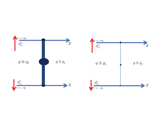
Figure 1: Left: An instanton configuration contributing to the differential on the MSW complex. The black regions indicate the locus where the field $\phi(x,\tau)$ varies vary significantly from the vacuum configurations $\phi_{i}$ or $\phi_{j}$. The length scale here is $\ell_{W}$, set by the superpotential $W$. Right: Viewed from a large distance compared to the length scale $\ell_{W}$ the instanton looks like a straight line $x=x_{0}$, where the vacuum changes discontinuously from vacuum $\phi_{i}$ to $\phi_{j}$. The nontrivial $\tau$-dependence of the instanton configuration, interpolating from a soliton $p_{1}$ to another soliton $p_{2}$ has been contracted to a single vertex located at $\tau=\tau_{0}$. This vertical line with a single vertex on it is the first example of a “web” in the web formalism.

Written out the boundary conditions for the $\zeta$-instanton equation are:

$$\lim_{x\to-\infty}\phi(x,\tau)=\phi_{i}\qquad\lim_{x\to+\infty}\phi(x,\tau)=\phi_{j}$$ (17)

$$\lim_{\tau\to-\infty}\phi(x,\tau)=\phi^{p_{1}}_{ij}(x)\qquad\lim_{\tau\to+\infty}\phi(x,\tau)=\phi^{p_{2}}_{ij}(x).$$ (18)

Following the rules of SQM, the matrix elements of the differential are obtained by counting the solutions with no reduced moduli, (i.e. the solutions with two moduli).

Remarks:

1. The complex (13) is not a standard mathematical Morse theory complex: $h$ is degenerate because of translation invariance. The critical set is ${\mathbb{R}}$, parametrizing the “center of mass” of the soliton. But we sum neither the cohomology nor the compactly supported cohomology of this critical set, as one would do in standard Morse theory. Rather, we attach a certain Clifford module to each critical locus. Physically this arises from the quantization of the “collective coordinates” associated with the center of mass of the soliton. The module has rank two. That is why each classical soliton contributes two perturbative groundstates in equation (13). In equation (50) below we have factored out this center of mass degree of freedom and hence each soliton leads to just one perturbative groundstate.

2. Supersymmetric quantum mechanics has two supersymmetries satsifying $\{Q,\bar{Q}\}=2H$. When the spatial domain is $D={\mathbb{R}}$ there are more symmetries in the problem, such as translational symmetry along ${\mathbb{R}}$, not manifest from the general SQM viewpoint. Consequently, when the spatial domain is ${\mathbb{R}}$ the LG model has (2,2) supersymmetry:

   $$\begin{split}\{Q_{+},\bar{Q}_{+}\}=H+P\qquad&\qquad\{Q_{+},Q_{-}\}=\bar{Z}\\ \{Q_{-},\bar{Q}_{-}\}=H-P\qquad&\qquad\{\bar{Q}_{+},\bar{Q}_{-}\}=Z.\\ \end{split}$$ (19)

   The supersymmetries of the SQM are of the form

   $${\cal Q}_{\zeta}:=Q_{-}-\zeta^{-1}\bar{Q}_{+},~{}~{}\bar{{\cal Q}}_{\zeta}:=\bar{Q}_{-}-\zeta Q_{+}.$$ (20)

   The vacua of the model $\phi_{i}\in{\mathbb{V}}$ preserve four supersymmetries. The $\zeta$-soliton equation is the ${\cal Q}_{\zeta}$ (or $\bar{\cal Q}_{\zeta}$)-fixed point equation for stationary classical field configurations. Solutions of these equations preserve two out of the four supersymmetries. The $\zeta$-instanton equation is an equation for the theory in Euclidean signature and preserves only one supersymmetry, namely ${\cal Q}_{\zeta}$. When $D$ is a half-line or an interval, with suitable boundary conditions, only the two-dimensional supersymmetry algebra generated by ${\cal Q}_{\zeta}$ and $\bar{{\cal Q}}_{\zeta}$ will be preserved.

3. Now comes an important physics point: The theory is massive with a length scale $\ell_{W}$ corresponding to the inverse of the lightest soliton mass. Physical correlations should decay exponentially beyond that scale. We can picture the solitons and instantons as in Figure 1.

4. The $\zeta$-instanton equation has also appeared in the literature on the relation of matrix models and Landau-Ginzburg models [17, 5]. It also appears in the literature on BPS domain walls in four-dimensional supersymmetric theories [1, 10]. There are even some exact solutions available in the literature [14].

1.4 LG Models On A Half-Plane And The Strip

1.4.1 Boundary Conditions

If $D$ has a left-boundary $x_{\ell}\leq x$ or a right boundary $x\leq x_{r}$ at finite distance then we need to put boundary conditions to get a good Morse theory, or QFT.

1. At $x=x_{\ell},x_{r}$, the boundary value $\phi^{\partial}$ must be valued in a maximal Lagrangian submanifold ${\cal L}_{\ell},{\cal L}_{r}$ of $X$ in order to have elliptic boundary conditions for the Dirac equation on the fermions.

2. The theory is simplest when the Lagrangian submanifolds are exact: $\iota^{*}(\lambda)=dk$, for a single-valued function $k$. Indeed, the Morse function (6) is replaced by $h\to h\pm k(\phi^{\partial})$, where the sign is for the negative/positive half-plane, respectively. Note that $k$ can thus be interpreted physically as a boundary superpotential.

We are certainly interested in $X$ which is noncompact (since we want $W$ to be nontrivial) and we are typically interested in noncompact Lagrangians. Now, we want to have well-defined spaces of quantum states on an interval ${\cal H}_{{\cal L}_{\ell},{\cal L}_{r}}$, invariant under separate Hamiltonian symplectomorphisms of the left and right branes. (These are mirror dual to gauge transformations on the branes of the B-model.)

The generators of the MSW complex in this case can be identified with the intersection points

$${\cal L}_{\ell}^{(\Delta x)}\cap{\cal L}_{r}$$ (21)

where we regard the $\zeta$-soliton equation (8) as a flow in $x$ and ${\cal L}^{(\Delta x)}$ means the flow has been applied for a range $(\Delta x)$.

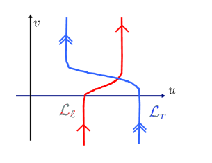
Figure 2: A pair of Lagrangian submanifolds ${\cal L}_{\ell}$, $\L_{r}$ embedded in the $u-v$ plane. ${\cal L}_{\ell}$ and ${\cal L}_{r}$ intersect at the one point indicated. $u$ is plotted horizontally and we assume that ${\cal L}_{\ell}$, ${\cal L}_{r}$ are embedded in the half-plane $u>0$.

But now there is a problem: Intersection points can go to infinity as the length of the interval is changed (or if independent Hamiltonian symplectomorphisms are applied to left and right branes). As an example, consider $\zeta^{-1}W={\rm i}\phi^{2}$ and consider the candidate left and right branes shown in Figure 2. We regard the $\zeta$-soliton equation as a flow in $x$, and if $\phi=u+{\rm i}v$ is the decomposition into real and imaginary parts then

$$\partial_{x}u=u\qquad\partial_{x}v=-v$$ (22)

Therefore, the flow in $x$ of ${\cal L}_{\ell}$ will not intersect ${\cal L}_{r}$ for sufficiently large $x$. Therefore there will be supersymmetric states for small width of $[x_{\ell},x_{r}]$ but none for large width of $[x_{\ell},x_{r}]$. This is potentially an interesting feature for a physicist studying supersymmetry breaking, but it is a bug for the kind of “partial topological field theory” we are studying.

In [9] we find that there are two distinct criteria we could impose on the allowed Lagrangians to avoid the above problem. One solution is to restrict the left and right branes to be positively and negatively $W$-dominated, respectively. A brane supported on ${\cal L}$ is positively (negatively) $W$-dominated if ${\rm Im}(\zeta^{-1}W)\to\pm\infty$ as $\phi$ goes to infinity along ${\cal L}$. Alternatively, one can restrict the Lagrangians to be Branes of class $T_{\kappa}$: Choose a phase $\kappa\not=\pm\zeta$, and constants $c,c^{\prime}$. The precise choices don’t matter too much, although which component of the circle $\kappa$ sits in is significant. Branes of class $T_{\kappa}$ are based on Lagrangians which project under $W$ to a semi-infinite rectangle in the $W$-plane:

$$\begin{split}|\mathrm{Re}\,(\kappa^{-1}W)|&\leq c\cr\mathrm{Im}\,(\kappa^{-1}W)&\geq c^{\prime},\\ \end{split}$$ (23)

as in Figure 3. In the second approach branes on both the left and right boundaries are taken to be in class $T_{\kappa}$. Now, under the $x$-flow of the $\zeta$-soliton equation we have

$$\frac{d}{dx}\mathrm{Re}\,(\kappa^{-1}W)=-\frac{1}{2}\{{\rm Re}(\zeta^{-1}W),{\rm Re}(\kappa^{-1}W)\}=\frac{1}{4}{\rm Im}(\frac{\zeta}{\kappa})|dW|^{2}$$ (24)

Then, points at infinity flow very fast out of the rectangle and hence intersection points ${\cal L}_{\ell}^{(\Delta x)}\cap{\cal L}_{r}$ always sit in a bounded region and cannot escape to infinity.

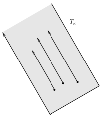
Figure 3: The rays in the complex $W$-plane that start at critical points and all run in the $\i\kappa$ direction fit into the semi-infinite strip $T_{\kappa}$, which is shown as a shaded region.

1.4.2 LG Ground States On A Half-Line

Now we consider the theory on the positive half-plane. We choose $\zeta$ so that it does not coincide with any of the $\zeta_{ij}$ defining the solitons for $D={\mathbb{R}}$. What are the groundstates preserving ${\cal Q}_{\zeta}$ supersymmetry?

The MSW complex $\mathbb{M}_{{\cal L}_{\ell},j}$ is generated by the $\zeta$-solitons on the half-plane satisfying the above boundary conditions. The grading on the complex is again given by fermion number but finding a formula for the fermion number is a little nontrivial. We only know how to describe it when $X$ is Calabi-Yau. In this case case we define

$$e^{\i\vartheta}=\frac{\mathbf{vol}}{\Omega|_{{\cal L}}}$$ (25)

(where $\Omega$ trivializes $K_{X}$ and is normalized so that $\Omega\bar{\Omega}$ is the volume form on $X$) and we need to be able to define a single-valued logarithm $\vartheta$. (That is, the Maslov index must vanish.) In this case we define the fermion number (on the interval) to be:

$$f=-\frac{1}{2}\eta({\mathcal{D}})-2\frac{\varphi_{r}-\varphi_{\ell}}{2\pi}.$$ (26)

where $\varphi=\vartheta(\phi^{\partial})$. On a half-line we drop $\varphi_{r}$ or $\varphi_{\ell}$ as appropriate.

The differential on the complex is given by counting $\zeta$-instantons. The picture of the instantons on the half-plane is shown in Figure 4

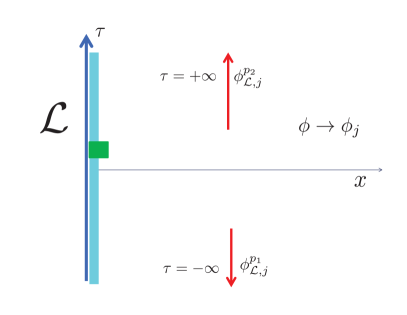
Figure 4: An instanton in the complex $\mathbb{M}_{{\cal L},j}$. The solitons corresponding to $p_{1},p_{2}\in{\cal L}\cap R^{\zeta}_{j}$, where $R^{\zeta}_{j}$ is the right Lefshetz thimble, are exponentially close to the vacuum $\phi_{j}$ except for a small region, shown in turquoise, of width $\ell_{W}$. In addition, the instanton transitions from one soliton to another in a time interval of length $\ell_{W}$, indicated by the green square. At large distances the green square becomes the $0$-valent vertex used in half-plane webs.

1.4.3 LG Ground States On The Strip

The story on the strip is very similar to that on the half-plane, but there is an interesting wrinkle that provides a nice example where naive categorification of formulae for BPS degeneracies fails: We consider the LG theory on ${\mathbb{R}}\times[x_{\ell},x_{r}]$. When $|x_{r}-x_{\ell}|\gg\ell_{W}$ the $\zeta$-solitons must nearly “factorize” so there is a natural isomorphism:

$$\mathbb{M}_{{\cal L}_{\ell},{\cal L}_{r}}\cong\oplus_{i\in{\mathbb{V}}}\mathbb{M}_{{\cal L}_{\ell},i}\otimes\mathbb{M}_{i,{\cal L}_{r}}.$$ (27)

So if we define the BPS degeneracy of the half-line solitons:

$$\mu_{{\cal L},i}:={{\rm Tr}}_{\mathbb{M}_{{\cal L},i}}e^{i\pi{\rm\textbf{F}}},$$ (28)

and similarly define $\mu_{i,{\cal L}}$ and $\mu_{{\cal L}_{\ell},{\cal L}_{r}}$, then the Euler-Poincaré principle guarantees

$$\mu_{{\cal L}_{\ell},{\cal L}_{r}}=\sum_{i\in{\mathbb{V}}}\mu_{{\cal L}_{\ell},i}\mu_{i,{\cal L}_{r}}.$$ (29)

Now, the naive categorification would state:

$$H^{*}(\mathbb{M}_{{\cal L}_{\ell},{\cal L}_{r}})\overset{?}{\cong}\oplus_{i\in{\mathbb{V}}}H^{*}(\mathbb{M}_{{\cal L}_{\ell},i})\otimes H^{*}(\mathbb{M}_{i,{\cal L}_{r}}).$$ (30)

Here we have used the natural differential on the tensor-product complex. It corresponds to the $\zeta$-instantons of Figure 5:

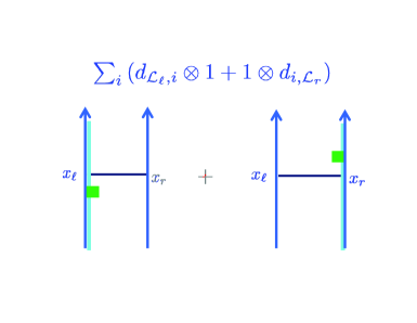
Figure 5: Naive differential on the strip.

As we will see, equation (30) is wrong. The reason is that there are other $\zeta$-instantons which also contribute to the physically correct differential. One example is a $\zeta$-instanton that looks like Figure 6. We will interpret this figure more precisely at the end of §2.1.1.

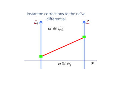
Figure 6: An instanton correction to the naive differential on the strip.

1.5 A Physicist’s View Of The Fukaya-Seidel Category

Finally, we sketch the Fukaya-Seidel (FS) category, at least the way a physicist would approach it (after benefiting from exposure to mathematical thinking on this topic).

Fix $\zeta$. Our objects will be branes based on Lagrangians in class $T_{\kappa}$, where $\kappa$ is in one of the two components of $U(1)-\{\pm\zeta\}$. Up to $A_{\infty}$ equivalence the category should only depend on the choice of component. The morphism space is the MSW complex $\mathbb{M}_{{\cal L}_{\ell},{\cal L}_{r}}$ generated by solutions of the $\zeta$-soliton equation. Then, to compute the differential $M_{1}$, we count $\zeta$-instantons with one-dimensional moduli space. (That is, zero-dimensional reduced moduli space.) To compute the higher $A_{\infty}$-products we follow the example of open string field theory in light-cone gauge. We divide up the interval into equal length subintervals and consider the diagram in Figure 7. Finally, we have to integrate over the moduli - the relative positions of the joining times. When the fermion numbers of the incoming and outgoing states are such that the amplitude is not trivially zero the expected dimension of the moduli space will be zero, and in fact the solutions will only exist for a finite set of critical values $\tau_{i}-\tau_{i+1}$ where the strings join. The amplitude is obtained by counting over the finite set of solutions to the $\zeta$-instanton equation.

Figure 7: A picture of the worldsheet of $n$ open strings all of width $w$ coming in from the past ($\tau=-\infty$) with a single open string of width $nw$ going out to the future ($\tau=+\infty$), familiar from the light-cone gauge formulation of string interactions. (a) There are $n-1$ values of $\tau$ at which two open strings combine to one. The linearly independent differences between these critical values of $\tau$ are the $n-2$ real moduli of this worldsheet. (b) The picture in (a) can be slightly modified in this fashion so that the worldsheet is smooth. The moduli are still the differences between the critical values of $\tau$.

The $A_{\infty}$-category we have sketched above is not precisely what we one finds in the literature. (See, for example [15].) Our understanding from experts is that something roughly along the lines of what we have written using the $\zeta$-instanton equations is understood to be the natural conceptual framework for defining the FS category, and that proofs along these lines will materialize in the literature in due course.

2 The Web Formalism

2.1 Boosted Solitons And $\zeta$-Webs

Now we would like to interpret more precisely the meaning of Figure 6.

2.1.1 Boosted Solitons

Recall that $\zeta$-instantons satisfy

$$\left(\frac{\partial}{\partial x}+{\rm i}\frac{\partial}{\partial\tau}\right)\phi^{I}=\frac{{\rm i}\zeta}{2}g^{I\bar{J}}\frac{\partial\bar{W}}{\partial\bar{\phi}{}^{\bar{J}}},$$ (31)

and we are interested in solutions for arbitrary phase $\zeta$. Recall too that $\zeta$-solitons on $D={\mathbb{R}}$ satisfy

$$\frac{{\mathrm{d}}}{{\mathrm{d}}x}\phi^{I}=g^{I\bar{J}}\frac{{\rm i}\zeta}{2}\frac{\partial\bar{W}}{\partial\bar{\phi}^{\bar{J}}}.$$ (32)

Moreover, with boundary conditions $(\phi_{i},\phi_{j})$ at $x=-\infty,+\infty$ solutions only exist for special phases ${\rm i}\zeta_{ji}$ given by the phase of the difference of critical values $W_{j}-W_{i}$.

We can nevertheless use solitons of type $ij$ to produce solutions of the $\zeta$-instanton equation on the Euclidean plane by taking the ansatz:

$$\phi_{ij}^{\rm boosted}(x,\tau):=\phi_{ij}^{\rm soliton}(\cos\theta x+\sin\theta\tau).$$ (33)

Since

$$\left(\frac{\partial}{\partial x}+{\rm i}\frac{\partial}{\partial\tau}\right)\phi_{ij}^{{\rm boosted},I}(x,\tau)=\frac{{\rm i}e^{{\rm i}\theta}\zeta_{ji}}{2}g^{I\bar{J}}\partial_{\bar{J}}\bar{W}(\phi_{ij}^{{\rm boosted}})$$ (34)

it follows that if we choose the rotation $\theta$ so that

$$e^{{\rm i}\theta}\zeta_{ji}=\zeta$$ (35)

then we obtain a solution to the $\zeta$-instanton equation. We call such solutions to the $\zeta$-instanton equation boosted solitons. A short computation shows that the “worldline” (i.e. the region where the solution is not exponential close to one of the vacua $\phi_{i}$ or $\phi_{j}$) is parallel to the complex number $z_{ij}:=z_{i}-z_{j}$ where $z_{i}=\zeta\bar{W}_{i}$. See Figure 8.

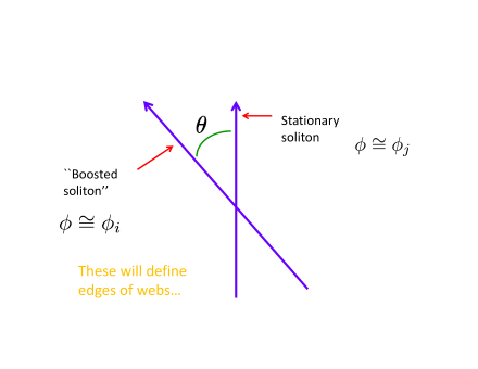
Figure 8: The boosted soliton. A short computation show that the “worldline” is parallel to the complex number $z_{ij}:=z_{i}-z_{j}$ where $z_{i}=\zeta\bar{W}_{i}$.

Now we can start to interpret the “extra” $\zeta$-instanton illustrated in Figure 6. The idea is that if the width of the interval is much larger than $\ell_{W}$ then the $\zeta$-instanton is well-approximated, away from the boundaries, by a boosted soliton. There is some kind of “emission amplitude” and “absorption amplitude” associated with the region where the boosted soliton joins the boundaries. In order to discuss these we first consider the $\zeta$-instanton equation on the plane, but with some unusual boundary conditions at infinity.

2.1.2 Fan Boundary Conditions

We would like to consider solutions to the $\zeta$-instanton equation that look like a collection of several boosted solitons at infinity. The boosted solitons will be obtained from a cyclically ordered set of solitons

$${\cal F}=\{\phi_{i_{1},i_{2}}^{p_{1}},\dots,\phi_{i_{n},i_{1}}^{p_{n}}\}.$$ (36)

ordered so that the worldlines of the boosted solitons have monotonically decreasing phase. We refer to such a set of solitons as a cyclic fan of solitons. We are interested in solutions to the $\zeta$-instanton equation which look like the corresponding boosted solitons as $z$ moves clockwise around a circle at infinity, as in Figure 9. Note this only makes sense when the phases of the successive differences $z_{i_{k},i_{k+1}}$ are clockwise ordered. We call such a sequence of vacua a cyclic fan of vacua.

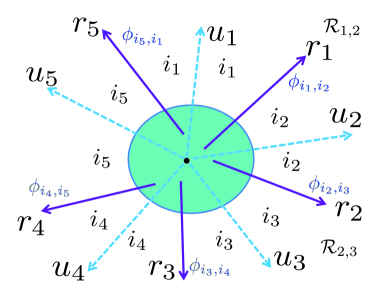
Figure 9: Boundary conditions on the $\zeta$-instanton equation defined by a cyclic fan of solitons. Here there are five boosted solitons and their worldlines near infinity are the rays $r_{1},\dots,r_{5}$. The boosted soliton solutions are exponentially close to the constant vacua near the rays $u_{1},\dots,u_{5}$ and can be modified there to produce true solutions to the $\zeta$-instanton equation.

If the index of a certain Dirac operator is positive then we expect, from index theory, that there will be $\zeta$-instantons which approach such a cyclic fan of solitons at infinity. In fact, as mentioned above, physicists studying domain wall junctions have established the existence of such solutions in some special cases [1, 10] and there are even examples of exact solutions [14]. We will assume that a moduli space of such solutions ${\cal M}({\cal F})$ exists. Based on physical intuition we expect these moduli spaces to satisfy two crucial properties:

1. Gluing: Under favorable conditions, two solutions which only differ significantly from fan solutions inside a bounded region can be glued together as in Figure 10 This process can be iterated to produce what we call $\zeta$-webs, shown in Figure 11:

2. Ends: The moduli space ${\cal M}({\cal F})$ can have several connected components. Some of these components will be noncompact, and the “ends,” or “boundaries at infinity,” of the moduli space will be described by $\zeta$-webs.

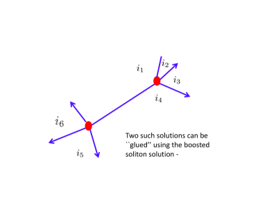
Figure 10: Gluing two solutions with fan boundary conditions to produce a new solution with fan boundary conditions. The red regions indicate where the solution deviates significantly from the boosted solitons and the vacua. When the “centers” of the two $\zeta$-instantons are far separated the approximate, glued, field configuration can be corrected to a true solution.

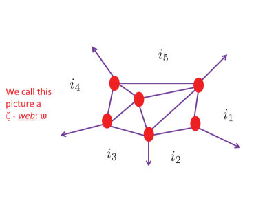
Figure 11: Several solutions can be glued together to produce a $\zeta$-web solution

The compact connected components of ${\cal M}({\cal F})$-webs are called $\zeta$-vertices. We are most interested in the $\zeta$-vertices of dimension zero: These will contribute to the path integral of the LG model with fan boundary conditions provided the fermion number of the outgoing states sums to $2$. We claim that counting such points for fixed fans of solitons produces interesting integers that satisfy $L_{\infty}$ identities. We will state that claim a bit more precisely later. This picture is the inspiration for the web-formalism, to which we turn next. It will give us the language to state the above claim in more precise terms.

2.2 The Web Formalism On The Plane

We now switch to a mathematical formalism that we call the web-based formalism for describing the above physics.

2.2.1 Planar Webs And Their Convolution Identity

Definition: The vacuum data is the pair $({\mathbb{V}},z)$ where ${\mathbb{V}}$ is a finite set called the set of vacua and $z:{\mathbb{V}}\to\mathbb{C}$ defines the vacuum weights.

The vacua are denoted $i,j,\dots\in{\mathbb{V}}$. The vacuum weight associated to $i$ is denoted $z_{i}$. The vacuum weights $\{z_{i}\}$ are assumed to be in general position. This means

$$\{z_{1},\dots,z_{N}\}\in{\cal V}:=\mathbb{C}^{N}-\mathfrak{E}$$ (37)

where $\mathfrak{E}$ is the exceptional set. The latter is defined to be collections of vacuum weights that satisfy at least one of the following three criteria: (1) $z_{ij}=0$ for some $i\not=j$ or (2) three distinct vacuum weights are colinear or (3) the weights allow the construction of an exceptional web. (Once we define webs below we can define exceptional webs to be those whose deformation space has a dimension larger than the expected dimension $2V-E$.)

Definition: A plane web is a graph in ${\mathbb{R}}^{2}$, together with a coloring of the faces by vacua such that the labels across each edge are different and moreover, when oriented with $i$ on the left and $j$ on the right the edge is straight and parallel to the complex number $z_{ij}:=z_{i}-z_{j}$. We take plane webs to have all vertices of valence at least two.

Definition The deformation type of a web is the equivalence class under stretching of internal edges and overall translation. There is a moduli space of deformation types and it can be oriented. We denote an oriented deformation type by $\mathfrak{w}$.

An example of two different deformation types of web is shown in Figure 12. In the web formalism and the related homotopical algebra there are many tricky sign issues, ultimately tracing back to the need to choose oriented deformation types of webs. Getting the signs right is a highly technical business and we will avoid it altogether in these notes. That is not to say that the signs are unimportant - they most certainly are! In [9] signs are taken into account with great care.

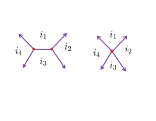
Figure 12: The two webs shown here are considered to be different deformation types, even though the web on the left can clearly degenerate to the web on the right.

Next, we introduce some notation for certain fans of vacua associated to a web. Recall that a fan of vacua is a cyclically ordered set of vacua so that successive edges are clockwise ordered. We can associate two kinds of fans of vacua to a web $\mathfrak{w}$:

1. The local fan of vacua at a vertex $v\in\mathfrak{w}$ is denoted $I_{v}(\mathfrak{w})$.

2. The fan of vacua at infinity is denoted $I_{\infty}(\mathfrak{w})$.

See Figure 13 for examples.

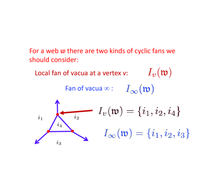
Figure 13: Illustrating the local fan of vacua and the fan of vacua at infinity for a web $\mathfrak{w}$.

Now we introduce the key construction of a convolution of webs: Suppose we have two webs $\mathfrak{w}$ and $\mathfrak{w}^{\prime}$ such that there is a vertex $v$ of $\mathfrak{w}$ where we have

$$I_{v}(\mathfrak{w})=I_{\infty}(\mathfrak{w}^{\prime}).$$ (38)

Then define $\mathfrak{w}*_{v}\mathfrak{w}^{\prime}$ to be the deformation type of a web obtained by cutting out a small disk around $v$ and gluing in a suitably scaled and translated copy of the deformation type of $\mathfrak{w}^{\prime}$. The procedure is illustrated in Figure 14. The upshot is that if ${\cal W}$ is the free abelian group generated by oriented deformation types of webs then convolution defines a product

$${\cal W}\times{\cal W}\to{\cal W}$$ (39)

(making it a “pre-Lie algebra” in the sense of [4]).

Figure 14: Illustrating the convolution of a web $\mathfrak{w}$ with internal vertex $v$ having a local fan $I_{v}(\mathfrak{w})=\{j_{1},j_{2},j_{3},j_{4}\}$ with a web $\mathfrak{w}^{\prime}$ having a fan at infinity $I_{\infty}(\mathfrak{w}^{\prime})=\{j_{1},j_{2},j_{3},j_{4}\}$.

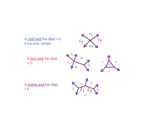
Figure 15: Illustrating rigid, taut, and sliding webs with $0$, $1$, and $2$ internal degrees of freedom. Here $d(\mathfrak{w})$ refers to the dimension of the reduced moduli space of the web, that is the dimension of the moduli space quotiented by the action of translation.

Let us now consider the taut webs. These are, by definition, those with only one internal degree of freedom. That is, the moduli space of the taut webs is three-dimensional. See Figure 15. We define the taut element $\mathfrak{t}\in{\cal W}$ to be the sum over all the taut webs:

$$\mathfrak{t}:=\sum_{d(\mathfrak{w})=3}\mathfrak{w}.$$ (40)

The key fact about taut webs is that

$$\mathfrak{t}*\mathfrak{t}=0.$$ (41)

The proof is that if we expand this out then we can group products in pairs which cancel. The pairs correspond to opposite ends of a moduli space of “sliding” webs, with two internal degrees of freedom. The idea is illustrated in Figure 16:

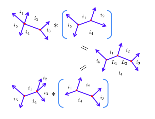
Figure 16: The two boundaries of the deformation type of the sliding web shown on the right correspond to different convolutions shown above and below. If we use the lengths $L_{1},L_{2}$ of the edges as coordinates then the orientation from the top convolution is $dL_{2}\wedge dL_{1}$. On the other hand the orientation from the bottom convolution is $dL_{1}\wedge dL_{2}$ and hence the sum of these two convolutions is zero. This is the key idea in the demonstration that $\mathfrak{t}*\mathfrak{t}=0$.

2.2.2 Representation Of Webs

Definition: A representation of webs is a pair ${\cal R}=(\{R_{ij}\},\{K_{ij}\})$ where $R_{ij}$ are ${\mathbb{Z}}$-graded ${\mathbb{Z}}$-modules defined for all ordered pairs $ij$ of distinct vacua and $K_{ij}$ is a degree $-1$ symmetric perfect pairing

$$K_{ij}:R_{ij}\otimes R_{ji}\to{\mathbb{Z}}.$$ (42)

Given a representation of webs, we define a representation of a cyclic fan of vacua $I=\{i_{1},i_{2},\dots,i_{n}\}$ to be

$$R_{I}:=R_{i_{1},i_{2}}\otimes R_{i_{2},i_{3}}\otimes\cdots\otimes R_{i_{n},i_{1}}$$ (43)

when $I$ is the cyclic fan at a vertex of a web we refer to $R_{I_{v}(\mathfrak{w})}$ to as the representation of the vertex. Elements of $R_{I_{v}(\mathfrak{w})}$ are called interior vectors.

Next we collect the representations of all possible vertices by forming

$$R^{\rm int}:=\oplus_{I}R_{I}$$ (44)

where the sum is over all cyclic fans of vacua. We include $I=\emptyset$ and define $R_{\emptyset}={\mathbb{Z}}$. We want to define a map

$$\rho(\mathfrak{w}):TR^{\rm int}\to R^{\rm int}$$ (45)

where for any ${\mathbb{Z}}$-module $M$ we define the tensor algebra to be

$$TM:=M\oplus M^{\otimes 2}\oplus M^{\otimes 3}\oplus\cdots$$ (46)

In fact, the operation will be graded-symmetric so it descends to a map from the symmetric algebra $SR^{\rm int}\to R^{\rm int}$.

We now define the contraction operation: We take $\rho(\mathfrak{w})[r_{1},\dots,r_{n}]$ to be zero unless $n=V(\mathfrak{w})$, the number of vertices of $\mathfrak{w}$, and there exists an order $\{v_{1},\dots,v_{n}\}$ for the vertices of $\mathfrak{w}$ such that $r_{a}\in R_{I_{v_{a}}(\mathfrak{w})}$. If such an order exists, we will define our map

$$\rho(\mathfrak{w}):\otimes_{v\in{\cal V}(\mathfrak{w})}R_{I_{v}(\mathfrak{w})}\to R_{I_{\infty}(\mathfrak{w})}$$ (47)

as the application of the contraction map $K$ to all internal edges of the web. Here ${\cal V}(\mathfrak{w})$ is the set of vertices of $\mathfrak{w}$. Indeed, if an edge joins two vertices $v_{1},v_{2}\in{\cal V}(\mathfrak{w})$ then if $R_{I_{v_{1}}(\mathfrak{w})}$ contains a tensor factor $R_{ij}$ it follows that $R_{I_{v_{2}}(\mathfrak{w})}$ contains a tensor factor $R_{ji}$ and these two factors can be paired by $K$ as shown in Figure 17.

Figure 17: The internal lines of a web naturally pair spaces $R_{i_{1},i_{2}}$ with $R_{i_{2},i_{1}}$ in a web representation, as shown here.

It is not difficult to see that the convolution identity $\mathfrak{t}*\mathfrak{t}=0$ implies that $\rho(\mathfrak{t})$ satisfies the axioms of an $L_{\infty}$ algebra $\rho(\mathfrak{t}):TR^{\rm int}\to R^{\rm int}$:

$$\sum_{{\rm Sh}_{2}(S)}\epsilon_{S_{1},S_{2}}~{}\rho(\mathfrak{t})[\rho(\mathfrak{t})[S_{1}],S_{2}]=0$$ (48)

where we sum over 2-shuffles of the ordered set $S=\{r_{1},\dots,r_{n}\}$ and $\epsilon_{S_{1},S_{2}}$ is a sign factor discussed at length in [9].

Definition: An interior amplitude is an element $\beta\in R^{\rm int}$ of degree $+2$ so that if we define $e^{\beta}\in TR^{\rm int}\otimes\mathbb{Q}$ by the exponential series then

$$\rho(\mathfrak{t})(e^{\beta})=0.$$ (49)

Definition: A Theory ${\cal T}$ consists of a set of vacuum data $({\mathbb{V}},z)$, a representation of webs ${\cal R}=(\{R_{ij}\},\{K_{ij}\})$ and an interior amplitude $\beta$.

The simplest case of the $L_{\infty}$ equation implies there is a component of $\beta$ in $R_{ij}\otimes R_{ji}$ sastifying a quadratic equation. Using $K$ we can interpret this component of $\beta$ as a map $Q_{ij}:R_{ij}\to R_{ij}$ of degree one that squares to zero. Thus, the $R_{ij}$ become chain complexes. It is also worth noting that if $\beta$ is an interior amplitude and we define $\rho_{\beta}(\mathfrak{w})[r_{1},\dots,r_{\ell}]:=\rho(\mathfrak{w})[r_{1},\dots,r_{\ell},e^{\beta}]$ then $\rho_{\beta}(\mathfrak{t}):TR^{\rm int}\to R^{\rm int}$ also satisfies the $L_{\infty}$ Maurer-Cartan equation and in this way we obtain moduli spaces of Theories.

The mathematical structure we have just described is realized in the Landau-Ginzburg model as follows:

1. Vacua: ${\mathbb{V}}$ is the set of critical points of $W$.

2. Vacuum weights: $z_{i}=\zeta\bar{W}_{i}$

3. Web representation:

   $$R_{ij}:=\oplus_{p\in{\cal S}_{ij}}{\mathbb{Z}}\Psi^{f+1}(p)$$ (50)

   is the MSW complex, where we take the upper fermion number for each soliton $p$. The contraction $K$ is defined by the path integral and is a kind of inner product on the solitons.

4. Interior amplitude: Suitably interpreted, the path integral leads to a counting of $\zeta$-instantons with fan boundary conditions and defines an element in $R^{\rm int}$ which is an interior amplitude $\beta$. This follows from localization of the path integral on the moduli space of $\zeta$-instantons and the fact that the path integral must create a ${\cal Q}_{\zeta}$-closed state. For details see Section §14 of [9].

2.2.3 Examples: Theories With Cyclic Weights

Two useful examples have ${\mathbb{V}}={\mathbb{Z}}/N{\mathbb{Z}}$. We break the cyclic symmetry and label vacua by $i\in\{0,\dots,N-1\}$ with weights:

$${\mathbb{V}}^{N}_{\vartheta}:z_{k}=e^{-{\rm i}\vartheta-\frac{2\pi{\rm i}}{N}k}\qquad k=0,\cdots N-1$$ (51)

(Although we have broken manifest cyclic symmetry all physically relevant results are cyclically symmetric. The web representations (53) and (56) below appear to violate this symmetry but that is not the case when one takes into account the “gauge freedom” in the definition of fermion numbers.)

The first example is ${\cal T}^{N}_{\vartheta}$ with a single chiral superfield and superpotential

$$W=\phi-e^{-{\rm i}N\vartheta}\frac{\phi^{N+1}}{N+1}.$$ (52)

The web-representation is

$$R_{ij} ={\mathbb{Z}}[1]\qquad i<j$$ (53)

$$R_{ij} ={\mathbb{Z}}\qquad i>j.$$ (54)

At a vertex of valence $n$ we have $\deg R_{I}=n-1$ and hence only 3-valent vertices contribute to the MC equations, so the only nonzero amplitudes are $\beta_{ijk}\in R_{ijk}$ for $0\leq i<j<k\leq N-1$. The $L_{\infty}$ equations come from the two taut webs of Figure 18 and are just:

$$\beta_{ijk}\beta_{ikt}-\beta_{ijt}\beta_{jkt}=0\qquad i<j<k<t$$ (55)

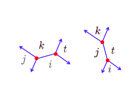
Figure 18: The two terms in the component of the $L_{\infty}$ equations for $i<j<k<t$. The resemblance to crossing symmetry is somewhat fortuitous. In other models the $L_{\infty}$ equations do not resemble crossing symmetry equations.

A more elaborate set of examples is provided by the mirror dual to the B-model on $\mathbb{C}\mathbb{P}^{N-1}$ with $SU(N)$ symmetry. This again has vacuum weights (51) but now we take

$$R_{ij} =A_{j-i}[1]\qquad i<j$$ (56)

$$R_{ij} =A_{N+j-i}\qquad i>j$$ (57)

where $A_{\ell}$ is the $\ell$-th antisymmetric power of a fundamental representation of $SU(N)$ and

$$K_{ij}(v_{1}\otimes v_{2})=\kappa_{ij}\frac{v_{1}\wedge v_{2}}{{\rm vol\,}}$$ (58)

where $\kappa_{ij}$ is a sign (determined by a rule in [9]) and ${\rm vol\,}$ denotes a choice of volume form on $\mathbb{C}^{N}$. An $SU(N)$-invariant ansatz for the interior amplitude reduces the $L_{\infty}$ MC equations to (55) above.

2.3 The Web Formalism On The Half-Plane

Fix a half-plane ${\cal H}\subset{\mathbb{R}}^{2}$ in the $(x,\tau)$ plane. Most of our pictures will take the positive or negative half-plane, $x\geq x_{\ell}$ or $x\leq x_{r}$, but it could be any half-plane.

Definition: Suppose $\partial{\cal H}$ is not parallel to any of the $z_{ij}$. A half-plane web in ${\cal H}$ is a graph in the half-plane which may have some vertices (but no edges) on the boundary. We apply the same rule as for plane webs: Label connected components of the complement of the graph by vacua so that if the edges are oriented with $i$ on the left and $j$ on the right then they are parallel to $z_{ij}$. Boundary vertices are allowed to be $0$-valent.

We can again speak of a deformation type of a half-plane web $\mathfrak{u}$. Now translations parallel to the boundary of ${\cal H}$ act freely on the moduli space. Once again we define half-plane webs to be rigid, taut, and sliding if the reduced dimension of the moduli space is $d(\mathfrak{u})=0,1,2$, respectively. Similarly, we can define oriented deformation type in an obvious way and consider the free abelian group ${\cal W}_{{\cal H}}$ of oriented deformation types of half-plane webs in the half-plane ${\cal H}$. Some examples where ${\cal H}={\cal H}_{L}$ is the positive half-plane are shown in Figure 19.

Figure 19: Four examples of taut positive-half-plane webs

There are now two new kinds of convolutions:

1. Convolution at a boundary vertex defines

$$*:{\cal W}_{{\cal H}}\times{\cal W}_{{\cal H}}\to{\cal W}_{{\cal H}}$$ (59)

2. Convolution at an interior vertex defines:

$$*:{\cal W}_{{\cal H}}\times{\cal W}\to{\cal W}_{{\cal H}}$$ (60)

We now define the half-space taut element:

$$\mathfrak{t}_{{\cal H}}:=\sum_{d(\mathfrak{u})=1}\mathfrak{u}.$$ (61)

The convolution identity is

$$\mathfrak{t}_{{\cal H}}*\mathfrak{t}_{{\cal H}}+\mathfrak{t}_{{\cal H}}*\mathfrak{t}_{p}=0.$$ (62)

where we now denote the planar taut element by $\mathfrak{t}_{p}$. The idea of the proof is the same as in the planar case. An example is shown in Figure 20.

Figure 20: An example of the identity on plane and half-plane taut elements. On the right is a sliding half-plane web. Above is a convolution of two taut half-plane webs with orientation $dy\wedge d\ell_{1}\wedge d\ell_{2}$, where $y$ is the vertical position of the boundary vertex and $\ell_{1},\ell_{2}$ are the lengths of the internal edges. Below is a convolution of a taut half-plane web with a taut plane web. The orientation is $dy\wedge d\ell_{2}\wedge d\ell_{1}$. The two convolutions determine the same deformation type but have opposite orientation, and hence cancel.

2.4 Categorification Of The 2D Spectrum Generator

Given a half-plane and a representation of webs we can introduce a collection of chain complexes $\widehat{R}_{ij}$ that will play an important role in what follows.

One way to motivate the $\widehat{R}_{ij}$ is to recall the Cecotti-Vafa-Kontsevich-Soibelman wall-crossing formula [3, 13] for the Witten indices/BPS degeneracies $\mu_{ij}={\rm Tr}_{R_{ij}}(-1)^{{\rm\textbf{F}}}$ of 2d solitons. The $\mu_{ij}$ were extensively studied in [6, 2, 3] where the wall-crossing phenomenon was first discussed. One way to state the wall-crossing formula uses the matrix of BPS degeneracies

$$\textbf{1}+\oplus_{z_{ij}\in{\cal H}}\widehat{\mu}_{ij}e_{ij}:=\bigotimes_{z_{ij}\in{\cal H}}(\textbf{1}+\mu_{ij}e_{ij})$$ (63)

where we assume there are $N$ vacua so we can identify ${\mathbb{V}}=\{1,\dots,N\}$, $e_{ij}$ are elementary $N\times N$ matrices, 1 is the $N\times N$ unit matrix, and in the tensor product we order the factors left to right by the clockwise order of the phase of $z_{ij}$. Continuous deformations of the Kähler metric $g_{I\bar{J}}$ and/or the superpotential $W$ in general lead to discontinuous changes in the number of solutions of equations (8), (10), and (11). The deformations of the Kähler metric do not change the indices $\mu_{ij}$ but changes in the superpotential that cross walls where three or more vacuum weights become colinear can indeed change the BPS index $\mu_{ij}$. The wall-crossing formula states that, nevertheless, the matrix (63) remains constant, so long as no ray through one of the $z_{ij}$ enters or leaves ${\cal H}$.

The matrix (63) is sometimes called the “spectrum generator.” We now “categorify” the spectrum generator, and define $\widehat{R}_{ij}$ from the formal product

$$\widehat{R}:=\oplus_{i,j=1}^{N}\widehat{R}_{ij}e_{ij}:=\bigotimes_{z_{ij}\in{\cal H}}({\mathbb{Z}}\cdot\textbf{1}+R_{ij}e_{ij})$$ (64)

Note that $\widehat{R}_{ii}={\mathbb{Z}}$ is concentrated in degree zero and $\widehat{R}_{ij}=0$ if $z_{ij}$ points in the opposite half-plane $-{\cal H}$. If $J=\{j_{1},\dots,j_{n}\}$ is a half-plane fan in ${\cal H}$ then we define

$$R_{J}:=R_{j_{1},j_{2}}\otimes\cdots\otimes R_{j_{n-1},j_{n}}$$ (65)

and $\widehat{R}_{ij}$ is just the direct sum over all $R_{J}$ for half-plane fans $J$ that begin with $i$ and end with $j$.

Remarks:

1. We can “enhance” the (categorified) spectrum generator $\widehat{R}$ with “Chan-Paton factors.” By definition, Chan-Paton data is an assignment $i\to{\cal E}_{i}$ of a ${\mathbb{Z}}$-graded module to each vacuum $i\in{\mathbb{V}}$. The modules ${\cal E}_{i}$ will be referred to as Chan-Paton factors. The enhanced spectrum generator is defined to be

   $$\widehat{R}({\cal E}):=\oplus_{i,j\in{\mathbb{V}}}\widehat{R}_{ij}({\cal E})e_{ij}:=\left(\oplus_{i\in{\mathbb{V}}}{\cal E}_{i}e_{ii}\right)\widehat{R}\left(\oplus_{j\in{\mathbb{V}}}{\cal E}_{j}e_{jj}\right)^{*}$$ (66)

2. Phase ordered products such as (63) have also appeared in many previous works on Stokes data, so the $R_{ij}$ can also be considered to be “categorified Stokes factors” and $\widehat{R}$ is an “categorified Stokes matrix.”

3. If we consider a family of theories where the rays $z_{ij}$ and $z_{jk}$ pass through each other then the categorified spectrum generator $\widehat{R}$ is in general not invariant, in striking contrast to (63). A categorified version of the Cecotti-Vafa-Kontsevich-Soibelman wall crossing formula is a rule for describing how $\widehat{R}$ changes. We will discuss such a rule in §3.5 below.

2.5 $A_{\infty}$-Categories Of Thimbles And Branes

2.5.1 The $A_{\infty}$-Category Of Thimbles

We now want to define the $A_{\infty}$-category of Thimbles, denoted ${\mathfrak{V}\mathfrak{a}\mathfrak{c}}$: Suppose we are given the data of a Theory ${\cal T}$ and a half-plane ${\cal H}$. Then ${\mathfrak{V}\mathfrak{a}\mathfrak{c}}$ has as objects the vacua $i,j,\dots\in{\mathbb{V}}$. As we will see,the objects of the category are better thought of as Thimble branes $\mathfrak{T}_{i},\mathfrak{T}_{j},\dots$, defined at the end of §2.5.2 below. The space of morphisms ${\rm Hom}(j,i)$ is simply

$${\rm Hom}(j,i):={\rm Hop}(i,j):=\widehat{R}_{ij}.$$ (67)

Here we have also introduced the notation ${\rm Hop}(i,j):={\rm Hom}(j,i)$ since many formulae in $A_{\infty}$-theory look much nicer when written in terms of ${\rm Hop}$.

We can enhance the category with Chan-Paton factors. The morphism spaces are simply the matrix elements of $\widehat{R}({\cal E})$:

$${\rm Hop}^{\cal E}(i,j):=\widehat{R}_{ij}({\cal E})={\cal E}_{i}\widehat{R}_{ij}{\cal E}_{j}^{*}.$$ (68)

The corresponding category is denoted ${\mathfrak{V}\mathfrak{a}\mathfrak{c}}({\cal E})$.

Now we need to define the $A_{\infty}$-multiplication in ${\mathfrak{V}\mathfrak{a}\mathfrak{c}}({\cal E})$ of an $n$-tuple of composable morphisms. As a first step, for any half-plane web $\mathfrak{u}$ we define a map

$$\rho(\mathfrak{u}):T\widehat{R}({\cal E})\otimes TR^{\rm int}\to\widehat{R}({\cal E})$$ (69)

It will be graded symmetric on the second tensor factor. As usual, we define the element

$$\rho(\mathfrak{u})[r^{\partial}_{1},\dots,r^{\partial}_{m};r_{1},\dots,r_{n}]$$ (70)

by contraction. We will abbreviate this to $\rho(\mathfrak{u})[P;S]$ where $P=\{r^{\partial}_{1},\dots,r^{\partial}_{m}\}$ and $S=\{r_{1},\dots,r_{n}\}$. We define $\rho(\mathfrak{u})[P;S]$ to be zero unless the following conditions hold:

• The boundary arguments match in order and type those of the boundary vertices: $r^{\partial}_{a}\in R_{J_{v^{\partial}_{a}}(\mathfrak{u})}({\cal E})$.

• We can find an order of the interior vertices ${\cal V}_{i}(\mathfrak{u})=\{v_{1},\dots,v_{n}\}$ of $\mathfrak{u}$ such that they match the order and type of the interior arguments: $r_{a}\in R_{I_{v_{a}}(\mathfrak{u})}$.

If the above conditions hold, we will simply contract all internal lines with $K$ and contract the Chan Paton elements of consecutive pairs of $r^{\partial}_{a}$ by the natural pairing ${\cal E}_{i}\otimes{\cal E}_{j}^{*}\to\delta_{ij}{\mathbb{Z}}$. With this definition in hand, we can check that the convolution identity for taut elements implies a corresponding identity for $\rho[\mathfrak{t}_{\cal H}]$:

$$\sum_{{\rm Sh}_{2}(S),{\rm Pa}_{3}(P)}\epsilon~{}\rho(\mathfrak{t}_{{\cal H}})[P_{1},\rho(\mathfrak{t}_{{\cal H}})[P_{2};S_{1}],P_{3};S_{2}]\\ +\sum_{{\rm Sh}_{2}(S)}\epsilon~{}\rho(\mathfrak{t}_{{\cal H}})[P;\rho(\mathfrak{t}_{p})[S_{1}],S_{2}]=0.$$ (71)

where ${\rm Pa}_{3}(P)$ is the set of partitions of the ordered set $P$ into an ordered set of three disjoint ordered sets, all inheriting the ordering of $P$. The signs are discussed in detail in [9]. We call (71) the $LA_{\infty}$ relations.

The most important consequence of these identities is that if we are given an interior amplitude $\beta$, we can immediately produce an $A_{\infty}$ category where the multiplication

$$\rho_{\beta}(\mathfrak{t}_{\cal H}):T\widehat{R}({\cal E})\to\widehat{R}({\cal E})$$ (72)

is defined by saturating all the interior vertices with the interior amplitude:

$$\rho_{\beta}(\mathfrak{t}_{\cal H})[r^{\partial}_{1},\dots,r^{\partial}_{m}]:=\rho(\mathfrak{t}_{\cal H})[r^{\partial}_{1},\dots,r^{\partial}_{m};e^{\beta}].$$ (73)

This has the effect of killing the second term in (71) and combining the first summand into the usual defining relations for an $A_{\infty}$-category. The product is illustrated in Figure 21.

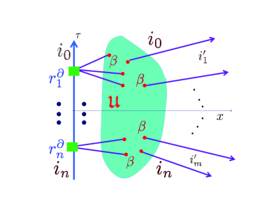
Figure 21: Illustrating the $A_{\infty}$-product on time-ordered boundary vectors $r^{\partial}_{1},\dots,r^{\partial}_{n}$. We sum over taut half-plane webs $\mathfrak{u}$, indicated by the green blob, and saturate all interior vertices with the interior amplitude $\beta$.

Remark: The conceptual meaning of (71) is that there is an $L_{\infty}$ morphism from the $L_{\infty}$ algebra $R^{\rm int}$ to the $L_{\infty}$ algebra of the Hochschild cochain complex of the $A_{\infty}$ category ${\mathfrak{V}\mathfrak{a}\mathfrak{c}}({\cal E})$. The paper [12] shows that in the present context the map is in fact an $L_{\infty}$ isomorphism.

2.5.2 The $A_{\infty}$-Category Of Branes

We define a Brane, denoted $\mathfrak{B}=({\cal E},{\cal B})$ to be a choice of Chan-Paton data ${\cal E}$ together with a boundary amplitude, that is, a degree $+1$ element

$${\cal B}\in\widehat{R}({\cal E})$$ (74)

that solves the Maurer-Cartan equations

$$\sum_{n=1}^{\infty}\rho_{\beta}(\mathfrak{t}_{\cal H})[{\cal B}^{\otimes n}]=\rho_{\beta}(\mathfrak{t}_{\cal H})[\frac{{\cal B}}{1-{\cal B}}]=0.$$ (75)

The category of Branes is denoted $\mathfrak{B}\mathfrak{r}$. It depends on the Theory ${\cal T}$ and the half-plane ${\cal H}$. Its objects are Branes $\mathfrak{B}=({\cal E},{\cal B})$ where ${\cal E}$ is any choice of Chan Paton data ${\cal E}$ and ${\cal B}$ is a compatible boundary amplitude. The space of morphisms from $\mathfrak{B}_{2}$ to $\mathfrak{B}_{1}$ is defined by simply modifying the enhanced spectrum generator to

$${\rm Hop}(\mathfrak{B}_{1},\mathfrak{B}_{2}):=\left(\oplus_{i}{\cal E}_{i}^{1}e_{ii}\right)\otimes\widehat{R}\otimes\left(\oplus_{i}{\cal E}_{i}^{2}e_{ii}\right)^{*}.$$ (76)

In order to define the composition of morphisms

$$\delta_{1}\in{\rm Hop}(\mathfrak{B}_{0},\mathfrak{B}_{1}),\quad\delta_{2}\in{\rm Hop}(\mathfrak{B}_{1},\mathfrak{B}_{2}),\dots,\delta_{n}\in{\rm Hop}(\mathfrak{B}_{n-1},\mathfrak{B}_{n})$$ (77)

we use the formula

$$M_{n}(\delta_{1},\dots,\delta_{n}):=\rho_{\beta}(\mathfrak{t}_{{\cal H}})\left(\frac{1}{1-{\cal B}_{0}},\delta_{1},\frac{1}{1-{\cal B}_{1}},\delta_{2},\dots,\delta_{n},\frac{1}{1-{\cal B}_{n}}\right).$$ (78)

Note that $M_{n}(\delta_{1},\dots,\delta_{n})\in{\rm Hop}(\mathfrak{B}_{0},\mathfrak{B}_{n})$. After some work (making repeated use of the fact that the ${\cal B}_{a}$ solve the $A_{\infty}$-Maurer-Cartan equation) one can show that the $M_{n}$ satisfy the $A_{\infty}$-relations and hence $\mathfrak{B}\mathfrak{r}$ is an $A_{\infty}$-category. In particular $M_{1}^{2}=0$ can be considered to be a differential (i.e. a nilpotent supercharge).

Remarks:

1. The multiplication (78) can be illustrated much as in Figure 21. The only difference is that now the boundary vectors $r_{s}^{\partial}$ don’t have to saturate all boundary vertices. Rather, boundary vertices between $r_{k}^{\partial}$ and $r_{k+1}^{\partial}$ can be saturated by the boundary amplitude ${\cal B}_{k}$.

2. For each vacuum $i$ we define the Thimble Brane $\mathfrak{T}_{i}$ to be the brane with CP data ${\cal E}(\mathfrak{T}_{i})_{j}=\delta_{i,j}{\mathbb{Z}}$ with boundary amplitude ${\cal B}(\mathfrak{T}_{i})=0$. Then the category of Thimbles ${\mathfrak{V}\mathfrak{a}\mathfrak{c}}$ is a full subcategory of $\mathfrak{B}\mathfrak{r}$.

2.5.3 Realization In The LG Model

Choose ${\cal H}$ to be the positive half-plane with boundary conditions set by a Lagrangian ${\cal L}\subset X$. The Chan-Paton data is given by the MSW complex:

$${\cal E}_{i}=\mathbb{M}_{{\cal L},i}$$ (79)

We consider amplitudes with boundary conditions shown in Figure 22. The counting of the number of $\zeta$-instantons satisfying these boundary conditions can be used to define an element ${\cal B}_{J}\in{\cal E}\otimes R_{J}\otimes{\cal E}^{*}$. As with the case of the interior amplitude, localization of the path integral to the moduli space of $\zeta$-instantons together with ${\cal Q}_{\zeta}$-closure of the state produced by the path integral implies that ${\cal B}$ is a boundary amplitude in the above sense.

In general the $M_{1}$-cohomology of ${\rm Hop}(\mathfrak{B}_{1},\mathfrak{B}_{2})$ is a space of ${\cal Q}_{\zeta}$-closed local boundary operators and the physical interpretation of $M_{n}(\delta_{1},\dots,\delta_{n})$ is that we are taking a kind of “operator product.” The ${\cal Q}_{\zeta}$ closure of the path integral implies that the $M_{n}$ satisfy the $A_{\infty}$-MC equation.

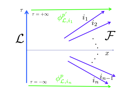
Figure 22: Boundary conditions for general half-plane instantons with fan boundary conditions at $x\to+\infty$ and solitons at $\tau\to\pm\infty$.

Remarks:

1. Spaces of local operators between some simple branes, such as Thimbles, for the theories with cyclic weights (Section §2.2.3 above) are described in Section §5.7 of [9]. In the theory with $SU(N)$ symmetry they are nontrivial representations of $SU(N)$.

2. If we want good morphism spaces associated to the interval $[x_{\ell},x_{r}]$ we need to restrict the class of Lagrangian submanifolds, as we have seen. In [9] it is argued that the suitable class of branes for which the web-formalism makes sense is the class of $W$-dominated branes for which ${\rm Im}(\zeta^{-1}W)\to+\infty$ at infinity. (For right-branes on boundaries of the negative half-plane we require ${\rm Im}(\zeta^{-1}W)\to-\infty$.) This class of branes includes the union of branes of class $T_{\kappa}$ for $\kappa$ in the open half-plane containing $\zeta$. However, in order to compare to the Fukaya-Seidel category one should restrict to a smaller class of branes, and it turns out that the subset of branes of class $T_{\zeta}$ will suffice. This might seem odd, since, as mentioned above, in our formulation of the Fukaya-Seidel category, we definitely want to use branes of type $T_{\kappa}$ with $\kappa\not=\pm\zeta$. The reason for the apparent discrepancy is explained in the next section.

2.6 Relation Of The Web-Based Formalism To The FS Category

Now we would like the relate the $A_{\infty}$-category constructed in the FS approach and in the web-based approach, say, for the positive half-plane. The web-based formalism applies to branes of class $T_{\zeta}$ and our description of the FS category applies to branes of class $T_{\kappa}$ with $\kappa\not=\pm\zeta$.

To relate the two we strongly use the rotational non-invariance of the $\zeta$-instanton equation and consider the FS category based on branes of class $T_{\zeta}$ but now the morphism spaces are defined by solving the equation on a horizontal strip, obtained from the vertical one by rotation by $\pi/2$. Thus, to define the morphisms of the FS category we use the MSW complex $\mathbb{M}_{\mathfrak{B}_{1},\mathfrak{B}_{2}}$ whose generators are solutions of the $\zeta$-instanton equation are invariant under translation in $x$ (but not in $\tau$). Now we can use branes of class $T_{\zeta}$ on the upper and lower boundary.

Figure 23: We count rigid $\zeta$-instantons in the funnel geometry to define an $A_{\infty}$-morphism between the FS category and the web-based category. The branes $\mathfrak{B}_{1},\mathfrak{B}_{2}$ are in class $T_{\zeta}$.

To relate the FS and web-based categories we now consider the $\zeta$-instanton equation on the funnel geometry of Figure 23. A state in the far past at $x\to-\infty$ on the strip is an incoming soliton, in the above sense. A state in the morphisms in the web-based formalism gives half-plane fan boundary conditions at infinity for the positive half-plane. But these two states determine boundary conditions for the $\zeta$-instanton equation on the space in Figure 23. We can therefore define a map

$${\cal U}:\mathbb{M}_{\mathfrak{B}_{1},\mathfrak{B}_{2}}\to{\rm Hop}(\mathfrak{B}_{1},\mathfrak{B}_{2})$$ (80)

The matrix elements of ${\cal U}$ are defined by counting $\zeta$-instantons in the funnel geometry. When we consider states of the same fermion number the expected dimension of the moduli space is dimension zero and the moduli space is expected to be a finite set of points.

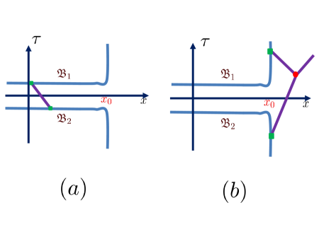
Figure 24: When the difference of fermion numbers of ingoing and outgoing states is $+1$ there will be a one-dimensional moduli space of $\zeta$-instantons. The two typical boundaries are indicated in (a) and (b). They lead to the two terms in the equation assuring that ${\cal U}$ is a chain map.

We claim that ${\cal U}$ is a chain map. To prove this we consider the one-dimensional moduli spaces of solutions to the $\zeta$-instanton equation between states whose fermion number differs by $1$. The two ends correspond to $\zeta$-instantons far down the strip - giving the differential on $\mathbb{M}_{\mathfrak{B}_{1},\mathfrak{B}_{2}}$ and taut webs far out on the positive half-plane, giving the differential on ${\rm Hop}(\mathfrak{B}_{1},\mathfrak{B}_{2})$, so

$${\cal U}\circ M_{1}^{\rm FS}-M_{1}^{\rm web}\circ{\cal U}=0$$ (81)

where $M_{1}$ denotes the differential on the morphisms in the $A_{\infty}$-category. Using similar arguments one can show that ${\cal U}$ can be extended to a full $A_{\infty}$-equivalence between the categories. For further details see Section §15 of [9].

2.7 Local Operators

The web formalism can also be used to determine spaces of local operators. To do this, we extend the $L_{\infty}$ algebra $R^{\rm int}$ by introducing a module $R_{i}\cong{\mathbb{Z}}$ for each vacuum $i\in{\mathbb{V}}$. In Section §9 of [9] we show that

$$R_{c}:=\oplus_{i\in{\mathbb{V}}}R_{i}\oplus R^{\rm int}$$ (82)

admits a natural $L_{\infty}$ algebra structure associated with doubly-extended webs. The extra data we add to a web are vertices with no edges attached. We argue that the cohomology of this complex is a space of local operators. The realization of these local operators in the Landau-Ginzburg models is a little subtle and is discussed in detail in Section §16 of [9]. The $R_{i}$ have generators corresponding to an insertion of “closed string” states on the circle with $\phi(x)=\phi_{i}$, while the $R_{I}\subset R^{\rm int}$ are related to twisted $\zeta$-solitons. That is, solitons on the circle where $\zeta(x)=\zeta e^{{\rm i}x}$. It turns out that the local operators described by the $M_{1}$-cohomology of ${\rm Hop}(\mathfrak{B}_{1},\mathfrak{B}_{2})$ and the cohomology of $R_{c}$ include certain kinds of disorder operators, novel to Landau-Ginzburg theories.

As an example, including suitable disorder operators helps resolve a puzzle in mirror symmetry: The standard $B$-model local operators of the $\mathbb{C}\mathbb{P}^{N-1}$ model do not correspond to the standard $A$-model local operators of the affine $SU(N)$ Toda model. Nevertheless, as shown in [9] the cohomology of (82) beautifully reproduces the space of $B$-model operators on $\mathbb{C}\mathbb{P}^{N-1}$.

3 Interfaces And Categorified Wall-Crossing

3.1 Motivation: Interfaces In Landau-Ginzburg Models

Suppose we have a family of superpotentials $W(\phi;c)$, parametrized by a point $c$ in a topological space $C$. Suppose $\wp:[x_{\ell},x_{r}]\to C$ is a continuous path. Then we can define a variant of LG theory based on an $x$-dependent superpotential:

$$W_{x}(\phi):=W(\phi;\wp(x)),$$ (83)

so that $W_{x}(\phi)$ is constant (in $x$) for $x\leq x_{\ell}$ and for $x\geq x_{r}$. Clearly this $1+1$ dimensional theory no longer has translational invariance. It does, however, still have two out of the four supersymmetries of LG theory. This is demonstrated most easily if we take the approach via Morse theory/SQM using the Morse function on ${\rm Map}({\mathbb{R}},X)$:

$$h=-\int_{{\mathbb{R}}}\left[\phi^{*}(\lambda)-\frac{1}{2}{{\rm Re}}(\zeta^{-1}W(\phi;\wp(x))dx\right].$$ (84)

Clearly the resulting theory has a kind of “defect” or “domain wall” localized near $[x_{\ell},x_{r}]$ interpolating between the left LG theory defined with superpotential $W_{x_{\ell}}(\phi)$ and the right LG theory defined with superpotential $W_{x_{r}}(\phi)$. We will refer to this as a (LG, supersymmetric) interface. The term “Janus” is also often used in the literature.

In the above setup we have a continuous family of vacuum weights

$$z_{i}(x)=\zeta\bar{W}_{x}(\phi_{i,x})$$ (85)

where the vacuum $i$ is parallel transported from the vacua in the theory at $x_{\ell}$ and $\phi_{i,x}$ are the critical points of the superpotential $W_{x}(\phi)$. The $\zeta$-instanton equation now becomes:

$$\left(\frac{\partial}{\partial x}+{\rm i}\frac{\partial}{\partial\tau}\right)\phi^{I}=\frac{{\rm i}\zeta}{2}g^{I\bar{J}}\frac{\partial\bar{W}}{\partial\bar{\phi}^{\bar{J}}}(\bar{\phi};\wp(x))$$ (86)

and $\zeta$-solitons are just $\tau$-independent solutions. The analog of boosted solitons have curved worldlines, as in Figure 25

Figure 25: An analog of the boosted soliton for the case of a supersymmetric interface.

Now, we would like to define a relation of the branes in the left theory to the branes in the right theory by “parallel-transporting” across the interface.

3.2 Abstract Formulation: Flat Parallel Transport Of Brane Categories

Suppose we have a “continuous family of Theories.” We use the term “Theory” in the sense of the web formalism. To make sense of this one must put a topology on the set of Theories. Note that the set of vacuum weights ${\cal V}$ of (37) carries a natural topology. Thus we can certainly speak of a continuous map

$$\wp:[x_{\ell},x_{r}]\to{\cal V}=\mathbb{C}^{N}-\mathfrak{E}$$ (87)

We call this a vacuum homotopy.

More generally, one can also define a sense in which web representations and the interior amplitudes change continuously. So, in general, we have a continuous family of Theories ${\cal T}(x)$ on $[x_{\ell},x_{r}]$. We would like to relate ${\cal T}^{\ell}={\cal T}(x_{\ell})$ to ${\cal T}^{r}={\cal T}(x_{r})$. More precisely, we want to define an $A_{\infty}$-functor

$${\cal F}(\wp):\mathfrak{B}\mathfrak{r}({\cal T}^{\ell},{\cal H})\rightarrow\mathfrak{B}\mathfrak{r}({\cal T}^{r},{\cal H})$$ (88)

where ${\cal H}$ is, say, the positive half-plane.

The functor ${\cal F}(\wp)$ is meant to be a categorical version of parallel transport by a flat connection. Thus we want:

1. An $A_{\infty}$-equivalence of functors:

   $${\cal F}(\wp_{1})\circ{\cal F}(\wp_{2})\cong{\cal F}(\wp_{1}\circ\wp_{2})$$ (89)

   for composable paths $\wp_{1},\wp_{2}$.

2. An $A_{\infty}$-equivalence of functors:

   $${\cal F}(\wp_{1})\cong{\cal F}(\wp_{2})$$ (90)

   for paths $\wp_{1},\wp_{2}$ homotopic in some suitable space.

We will show that one can construct such functors for “tame” vacuum homotopies, i.e. homotopies of the type (87). Flushed with success we then want to extend the construction to more general vacuum homotopies for paths of weights which cross the exceptional walls $\mathfrak{E}$. But you don’t always get what you want:

The existence of such a functor forces discontinuous changes of the web representation and the interior amplitude: This is the categorified version of wall-crossing.

The secret to constructing ${\cal F}(\wp)$ is the theory of Interfaces in the web-based formalism, to which we turn next.

3.3 Interface Webs And Composite Webs

3.3.1 The $A_{\infty}$-Category Of Interfaces

In order to understand the parallel transport of Brane categories it will actually be very useful to consider discontinuous jumps between Theories.

Given a pair of vacuum data $({\mathbb{V}}^{-},z^{-})$ and $({\mathbb{V}}^{+},z^{+})$ we can define an interface web by using the data on the negative and positive half-planes, respectively. Examples are shown in Figures 26 and 28 below. We can define the taut element $\mathfrak{t}^{-,+}$ and write a convolution identity. Next, if we are given left and right Theories $({\cal T}^{-},{\cal T}^{+})$ then we can define a representation of interface webs:

1. Chan-Paton factors are now labeled by a pair of vacua ${\cal E}_{j_{-},j^{\prime}_{+}}$.

2. At a boundary vertex we have the representation:

   $$R_{J}({\cal E}):={\cal E}_{j_{m},j^{\prime}_{1}}\otimes R_{J^{\prime}_{+}}^{+}\otimes{\cal E}_{j_{1},j^{\prime}_{n}}^{*}\otimes R_{J_{-}}^{-}.$$ (91)

   associated to the picture in Figure 26, where $J=(J_{-},J_{+}^{\prime})$.

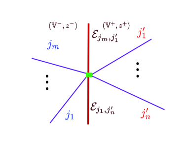
Figure 26: Conventions for Chan-Paton factors localized on interfaces. If representation spaces are attached to the rays then this figure would represent a typical summand in ${\rm Hom}(j_{m}j_{1}^{\prime},j_{1}j_{n}^{\prime})$. We order such vertices from left to right using the conventions of positive half-plane webs.

Now the categorified spectrum generator is given by the product

$$\widehat{R}({\cal E})=\left(\oplus_{i,i^{\prime}}{\cal E}_{ii^{\prime}}~{}e_{ii}\otimes e_{i^{\prime}i^{\prime}}\right)\left(\widehat{R}({\cal T}^{-},{\cal H}^{-})^{\rm tr}\otimes 1\right)\left(1\otimes\widehat{R}({\cal T}^{+},{\cal H}^{+})\right)\left(\oplus_{j,j^{\prime}}{\cal E}_{jj^{\prime}}~{}e_{jj}\otimes e_{j^{\prime}j^{\prime}}\right)^{*}$$ (92)

See Figure 26 for a typical summand.

Now an interface amplitude is a degree one element ${\cal B}^{-,+}\in\widehat{R}({\cal E})$ satisfying the $A_{\infty}$-MC equation:

$$\rho(\mathfrak{t}^{-,+})\left(\frac{1}{1-{\cal B}^{-,+}};e^{\beta_{-}};e^{\beta_{+}}\right)=0$$ (93)

We define an Interface to be a pair

$$\mathfrak{I}^{-,+}=({\cal E}^{-,+},{\cal B}^{-,+})$$ (94)

and we can define an $A_{\infty}$-category of Interfaces, denoted

$$\mathfrak{B}\mathfrak{r}({\cal T}^{-},{\cal T}^{+}).$$ (95)

The objects of $\mathfrak{B}\mathfrak{r}({\cal T}^{-},{\cal T}^{+})$ are Interfaces, for some choice of CP data and the space of morphisms between $\mathfrak{I}_{2}^{-,+}$ and $\mathfrak{I}_{1}^{-,+}$ is the natural generalization of (76):

$${\rm Hop}(\mathfrak{I}_{1}^{-,+},\mathfrak{I}_{2}^{-,+}):=\left(\oplus_{i,i^{\prime}}{\cal E}^{1}_{ii^{\prime}}~{}e_{ii}\otimes e_{i^{\prime}i^{\prime}}\right)\left(\widehat{R}({\cal T}^{-},{\cal H}^{-})^{\rm tr}\otimes 1\right)\left(1\otimes\widehat{R}({\cal T}^{+},{\cal H}^{+})\right)\left(\oplus_{j,j^{\prime}}{\cal E}^{2}_{jj^{\prime}}~{}e_{jj}\otimes e_{j^{\prime}j^{\prime}}\right)^{*}.$$ (96)

The $A_{\infty}$-multiplications are given by the natural generalization of equation (78): we just contract with the taut element $\mathfrak{t}_{{\cal H}}\to\mathfrak{t}^{-,+}$ and saturate all interior vertices with the left or right interior amplitude $\beta^{-},\beta^{+}$.

Figure 27: The only taut interface web when ${\cal T}^{\ell},{\cal T}^{r}$ are the trivial theory has two boundary vertices. The boundary amplitude is associated to a single boundary vertex: ${\cal B}\in{\cal E}\otimes{\cal E}^{*}$ is a morphism of ${\cal E}$ of degree one. There is only one taut web, shown above. The MC therefore says that ${\cal B}^{2}=0$. Thus an Interface between the trivial theory and itself is the same thing as a chain complex.

Remarks:

1. An Interface between the empty theory and itself is precisely the data of a chain complex. See Figure 27 for the explanation.

2. The identity Interface. A very useful example of an Interface is the identity Interface $\mathfrak{I}\mathfrak{d}\in\mathfrak{B}\mathfrak{r}({\cal T},{\cal T})$. The CP spaces are ${\cal E}(\mathfrak{I}\mathfrak{d})_{ij}=\delta_{i,j}{\mathbb{Z}}$ and

   $$\widehat{R}({\cal E})=\oplus_{i,j}\widehat{R}^{+}_{ij}\otimes\widehat{R}^{-}_{ji}e_{ij}\otimes e_{ij}$$ (97)

   where the superscripts $\pm$ indicate that $\widehat{R}$ is defined with respect to the positive, negative half-plane, respectively. To define the interface we take ${\cal B}_{{{\cal I}}}$ to have nonzero component only in summands of the form $R_{ij}\otimes R_{ji}$ corresponding to the fan $\{i,j;j,i\}$. The vertex looks like a straight line of a fixed slope running through the domain wall. The boundary amplitude is the element in $R_{ij}\otimes R_{ji}$ given by $K_{ij}^{-1}$. and the Maurer-Cartan equation is proved by Figure 28:

3. Landau-Ginzburg interfaces and branes in the product theory: In the context of Landau-Ginzburg models we can consider interfaces between a theory defined by $(X_{1},W_{1})$ on the negative half-plane and $(X_{2},W_{2})$ on the positive half-plane. By the doubling trick we would expect such interfaces to be related to branes for the positive half-plane of the theory based on $(\bar{X}_{1}\times X_{2},\bar{W}_{1}+W_{2})$. This is morally correct, but there are two closely related subtleties which should be pointed out. First, from the purely abstract formalism, if we try to relate Interface amplitudes for a pair of Theories ${\cal T}^{-},{\cal T}^{+}$ to boundary amplitudes for ${\cal T}^{-}\times{\cal T}^{+}$ we will, in general, fail: The vacua of the product theory are labeled by $(j_{-},j_{+})$ but the slopes of the edges of the webs are the slopes of $z_{j_{-}^{1},j_{-}^{2}}+z_{j_{+}^{1},j_{+}^{2}}$. In general half-plane fans for the product theory will have nothing to do with pairs of half-plane fans in the left and right theories. The two concepts will be equivalent, however, in the special case that the web representations are of the form

   $$R_{(j_{-}^{1},j_{+}^{1}),(j_{-}^{2},j_{+}^{2})}=\delta_{j_{-}^{1},j_{-}^{2}}R^{+}_{j_{+}^{1},j_{+}^{2}}\oplus\delta_{j_{+}^{1},j_{+}^{2}}R^{-}_{j_{-}^{1},j_{-}^{2}}.$$ (98)

   Second, on the Landau-Ginzburg side, if we literally take the product metric and the product superpotential then the Morse function $h_{1}+h_{2}$ is too degenerate: The critical manifolds are ${\mathbb{R}}\times{\mathbb{R}}$, corresponding to a center of mass collective coordinate for two separate solitons. We must perturb the theory by perturbing the superpotential with $\Delta W(\bar{\phi}_{1},\phi_{2})$. Generic perturbations will in fact produce MSW complexes giving web representations of the form (98).

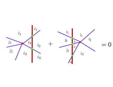
Figure 28: Examples of taut interface webs which contribute to the Maurer-Cartan equation for the identity interface $\mathfrak{I}\mathfrak{d}$ between a Theory and itself.

3.3.2 Composition Of Interfaces

A crucial new ingredient is that Interfaces can be composed. Suppose we have the situation shown in Figure 29 with a pair of Interfaces $\mathfrak{I}^{-,0}$ and $\mathfrak{I}^{0,+}$. We will produce a new Interface, denoted

$$\mathfrak{I}^{-,0}\boxtimes\mathfrak{I}^{0,+}\in\mathfrak{B}\mathfrak{r}({\cal T}^{-},{\cal T}^{+})$$ (99)

as shown in Figure 30.

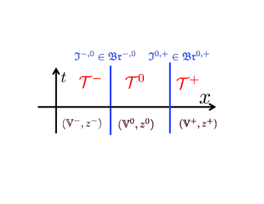
Figure 29: Two Interfaces between a sequence of three Theories.

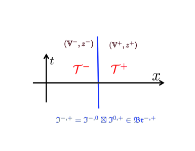
Figure 30: The Interface resulting from the “operator product” of the two Interfaces.

Figure 31: An example of a composite web, together with conventions for Chan-Paton factors. In this web the fan of vacua at infinity has $J_{\infty}(\mathfrak{c})=\{j^{\prime}_{1},\dots j^{\prime}_{n};j_{1},\dots,j_{m}\}$ Reading from left to right the indices are in clockwise order.

The key idea in the construction is to use “composite webs” $\mathfrak{c}=(\mathfrak{u}^{-},\mathfrak{s},\mathfrak{u}^{+})$. An example is shown in Figure 31. Again one can develop the whole web theory, write taut elements and a convolution identity. (The convolution identity has some novel features. See [9] for details.) The upshot is that the product Interface $\mathfrak{I}^{-,0}\boxtimes\mathfrak{I}^{0,+}$ has

1. Chan-Paton data:

   $${\cal E}(\mathfrak{I}^{-,0}\boxtimes\mathfrak{I}^{0,+})_{ii^{\prime}}:=\oplus_{i^{\prime\prime}\in{\mathbb{V}}^{0}}{\cal E}_{i,i^{\prime\prime}}^{-,0}\otimes{\cal E}_{i^{\prime\prime},i^{\prime}}^{0,+}$$ (100)

2. Interface amplitude:

   $${\cal B}(\mathfrak{I}^{-,0}\boxtimes\mathfrak{I}^{0,+}):=\rho_{\beta}(\mathfrak{t}_{c})\left[\frac{1}{1-{\cal B}^{-,0}};\frac{1}{1-{\cal B}^{0,+}}\right]$$ (101)

   where $\mathfrak{t}_{c}$ is the taut element for composite webs.

   Using the convolution identity (omitted here) one can show that it indeed satisfies the Maurer Cartan equations for an interface amplitude between the theories ${\cal T}^{-}$ and ${\cal T}^{+}$ with Chan-Paton spaces (100).

Now one can show that we have an $A_{\infty}$-bifunctor

$$\mathfrak{B}\mathfrak{r}({\cal T}^{-},{\cal T}^{0})\times\mathfrak{B}\mathfrak{r}({\cal T}^{0},{\cal T}^{+})\to\mathfrak{B}\mathfrak{r}({\cal T}^{-},{\cal T}^{+})$$ (102)

This is illustrated in Figure 32

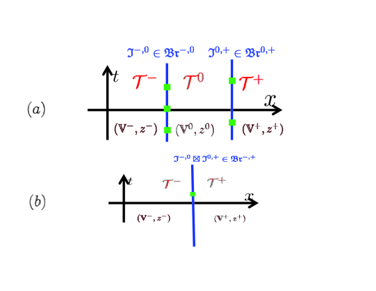
Figure 32: Illustrating the bi-functor property: We take the “OPE” of both local boundary operators on the interfaces, and of the interfaces, shown in (a), to produce a local operator on an interface, shown in (b).

An important special case is that where ${\cal T}^{-}$ is the trivial Theory so that $\mathfrak{B}\mathfrak{r}({\cal T}^{-},{\cal T}^{0})=\mathfrak{B}\mathfrak{r}({\cal T}^{0})$. Then we see that a $\boxtimes$ with a fixed Interface $\mathfrak{I}\in\mathfrak{B}\mathfrak{r}({\cal T}^{0},{\cal T}^{+})$ gives an $A_{\infty}$-functor on categories of Branes:

$$\mathfrak{B}\mathfrak{r}({\cal T}^{0})\times\mathfrak{B}\mathfrak{r}({\cal T}^{0},{\cal T}^{+})\to\mathfrak{B}\mathfrak{r}({\cal T}^{+})$$ (103)

Physically, we are moving a $0,+$ interface $\mathfrak{I}$ into a boundary and mapping a boundary condition for Theory ${\cal T}^{0}$ to one for Theory ${\cal T}^{+}$.

Thus, our quest for parallel transport of Brane categories will be fulfilled if we can find suitable Interfaces $\mathfrak{I}[\wp]$ associated with paths between theories ${\cal T}^{\ell}$ and ${\cal T}^{r}$.

3.3.3 An $A_{\infty}$ 2-Category Of Interfaces

A natural question to ask about the composition of Interfaces is whether it is associative. In fact, to define the composite webs we need to choose positions on the $x$-axis for the two domain walls as well as the position of the final interface. These positions can influence the set of composite webs. So we should really denote the product of Interfaces by

$$\left(\mathfrak{I}^{-,0}\boxtimes\mathfrak{I}^{0,+}\right)_{x^{-,0},x^{0,+},x^{-,+}}$$ (104)

However, one can show that the product only depends on these positions up to “homotopy equivalence.” The proof, which is somewhat long, involves developing a theory of webs which are time-dependent. Similarly, one can prove that the composition is associative, up to “homotopy equivalence.” All the details are in [9].

To define “homotopy equivalence” let us note that the $A_{\infty}$-structure of the category of Branes and Interfaces requires in part that the Hop spaces have a differential: If $\delta\in{\rm Hop}(\mathfrak{B}_{1},\mathfrak{B}_{2})$ then

$$M_{1}(\delta)=\rho_{\beta}(\mathfrak{t}_{{\cal H}})\left(\frac{1}{1-{\cal B}_{1}},\delta,\frac{1}{1-{\cal B}_{2}}\right)$$ (105)

and $M_{1}\circ M_{1}=0$, when the Hop spaces are composable. We can thus define a notion of homotopy equivalence of Branes (and entirely parallel definitions apply to Interfaces):

1. Two morphisms are homotopy equivalent if $\delta_{1}-\delta_{2}=M_{1}(\delta_{3})$.

2. Two Branes are homotopy equivalent, denoted, ${\cal B}\sim{\cal B}^{\prime},$ if there are two $M_{1}$-closed morphisms $\delta:{\cal B}\to{\cal B}^{\prime}$ and $\delta^{\prime}:{\cal B}^{\prime}\to{\cal B}$ which are inverses up to homotopy. That is:

$$M_{2}(\delta,\delta^{\prime})\sim\boldsymbol{\mathrm{Id}}\qquad\qquad M_{2}(\delta^{\prime},\delta)\sim\boldsymbol{\mathrm{Id}}.$$ (106)

where $\boldsymbol{\mathrm{Id}}$ is the natural identity in $\oplus_{i}{\cal E}_{i}\otimes{\cal E}_{i}^{*}$.

The net result of these observations is that we have defined what might be called an “$A_{\infty}$-2-category” structure:

1. The objects, or $0$-morphisms are the Theories.

2. The $1$-morphisms between two Theories are Interfaces $\mathfrak{I}^{-,+}$.

3. The $2$-morphisms between two $1$-morphisms are the boundary-changing operators on the Interface.

This is illustrated in Figure 33.

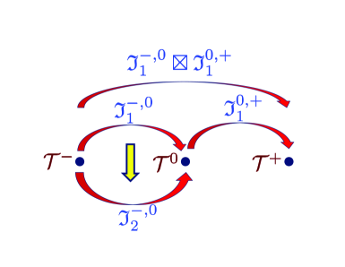
Figure 33: Illustrating the two category of Theories, Interfaces, and boundary operators.

3.4 An Example Of Categorical Transport

We will now sketch how one can actually construct a parallel transport interface for a tame vacuum homotopy:

$$\wp:x\mapsto\{z_{i}(x)\}\in\mathbb{C}^{N}-\mathfrak{E}$$ (107)

which does not cross the exceptional walls $\mathfrak{E}$. We assume $\wp(x)$ only varies on a compact set $[x_{\ell},x_{r}]$.

Our goal is to define an Interface

$$\mathfrak{I}[\wp]\in\mathfrak{B}\mathfrak{r}({\cal T}^{\ell},{\cal T}^{r})$$ (108)

so that if $\wp^{1}(x)\sim\wp^{2}(x)$ give homotopic paths of vacuum weights with fixed endpoints then $\mathfrak{I}[\wp^{1}]$ and $\mathfrak{I}[\wp^{2}]$ are homotopy-equivalent Interfaces, and such that if we compose two paths then

$$\mathfrak{I}[\wp^{1}]\boxtimes\mathfrak{I}[\wp^{2}]\sim\mathfrak{I}[\wp^{1}\circ\wp^{2}]$$ (109)

where $\sim$ means homotopy equivalence.

The key is to construct an analogous theory of curved webs where the $ij$ edges have tangents at $(x,\tau)$ parallel to $z_{i}(x)-z_{j}(x)$. One crucial new feature emerges for curved webs. Following the tangent vectors, sometimes the edges are forced to go to infinity at finite values of $x$. These special values of $x$ are known as binding points. We can have “future stable” binding points as in Figure 34 or “past stable” binding points as in Figure 35.

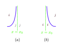
Figure 34: Near a future stable binding point $x_{0}$ of type $ij$ the edges separating vacuum $i$ from $j$ asymptote to the dashed green line $x=x_{0}$ in the future. Figures (a) and (b) show two possible behaviors of such lines. The phase $e^{-{\rm i}\vartheta(x)}z_{ij}$ rotates through the positive imaginary axis in the counterclockwise direction.

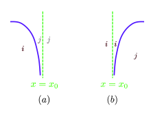
Figure 35: Near a past stable binding point $x_{0}$ of type $ij$ the edges separating vacuum $i$ from $j$ asymptote to the dashed green line $x=x_{0}$ in the past. Figures (a) and (b) show two possible behaviors of such lines. The phase $e^{-{\rm i}\vartheta(x)}z_{ij}$ rotates through the positive imaginary axis in the clockwise direction.

The binding points $x_{0}$ are characterized as the values of $x$ for which

$$z_{ij}(x_{0})\in{\rm i}{\mathbb{R}}_{+}$$ (110)

The future/past stability is determined by the sense in which ${\rm Re}\left(z_{ij}(x)\right)$ passes through zero as $x$ passes through $x_{0}$:

1. Future stable binding point: As $x$ increases past $x_{0}$ $z_{ij}(x)$ goes through the positive imaginary axis in the counter-clockwise direction.

2. Past stable binding point: As $x$ increases past $x_{0}$ $z_{ij}(x)$ goes through the positive imaginary axis in the clockwise direction.

Now we define Chan-Paton data of the desired Interface. For each binding point $x_{0}$ of type $ij$ introduce a matrix with chain-complex entries. It depends on whether $x_{0}$ is future-stable or past-stable:

$$S_{ij}(x_{0}):={\mathbb{Z}}\cdot\textbf{1}+R_{ij}e_{ij}\qquad\qquad future\ stable$$ (111)

$$S_{ij}(x_{0}):={\mathbb{Z}}\cdot\textbf{1}+R_{ji}^{*}e_{ij}\qquad\qquad past\ stable.$$ (112)

We will refer to $S_{ij}(x_{0})$ as a categorified $S_{ij}$-factor, or just as an $S_{ij}$-factor, for short. Then we define the Chan-Paton factors of the Interface to be:

$$\oplus_{i,j\in{\mathbb{V}}}{\cal E}_{i,j}e_{i,j}:=\bigotimes_{i\not=j}\bigotimes_{x_{0}\in\curlyvee_{ij}~{}\cup\curlywedge_{ij}}S_{ij}(x_{0})$$ (113)

where the tensor product on the RHS of (113) is an ordered product over binding points, ordered from left to right by increasing values of $x_{0}$. The amplitudes for the Interface are simply given by evaluating the taut curved web on the interior amplitude: $\rho(\mathfrak{t}_{\rm curved})(e^{\beta})$. (This formula needs some interpretation. See [9] for details.) In this way we get an Interface

$$\mathfrak{I}[\wp]\in\mathfrak{B}\mathfrak{r}({\cal T}^{\ell},{\cal T}^{r})$$ (114)

associated to the tame vacuum homotopy $\wp(x)$. It satisfies the desired properties for flat parallel transport.

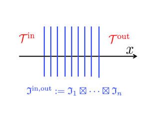
Figure 36: Breaking up the path $\wp$ into elementary paths we need only produce special interfaces for “trivial” transport, and for transport across $S$-walls.

Note that, thanks to the composition property (109), up to homotopy we can break up $\mathfrak{I}[\wp]$ as a product of Interfaces as in Figure 36. Therefore to construct $\mathfrak{I}[\wp]$ we need only construct then the Interfaces for crossing the $S_{ij}$ walls. These are denoted $\mathfrak{S}^{p,f}_{ij}$ for past and future stable crossings, respectively. The amplitudes can be described quite explicitly [9]. The functors $\mathfrak{B}\to\mathfrak{B}\boxtimes\mathfrak{S}^{p,f}_{ij}$ are closely related to mutations.

3.4.1 Categorified S-Wall-Crossing

We now return to one of our motivations from Section §1.2 above, namely the categorification of the $S$-wall crossing that plays such an important role in the theory of spectral networks [8]. Given an Interface $\mathfrak{I}^{-,+}$ associated with a path of theories the framed BPS degeneracies are, by definition:

$${\overline{\underline{\Omega}}}(\mathfrak{I}^{-,+},ij^{\prime}):={\rm Tr}_{{\cal E}(\mathfrak{I}^{-,+})_{ij^{\prime}}}e^{{\rm i}\pi{\rm\textbf{F}}}.$$ (115)

If we consider a path $\wp_{x}$ whose endpoint terminates with $z(x)$, and that crosses an $ij$ binding point as $x$ increases past $x_{0}$ (and hence $z(x)$ crosses an $S_{ij}$-wall) then the matrix of Witten indices

$$F[\wp_{x}]:=\sum_{k,\ell}{\overline{\underline{\Omega}}}(\mathfrak{I}[\wp_{x}],k,\ell)e_{k,\ell}.$$ (116)

jumps by

$$F\mapsto\begin{cases}F\cdot(\textbf{1}+\mu_{ij}e_{ij})&x_{ij}\in\curlywedge_{ij}\\ F\cdot(\textbf{1}-\mu_{ji}e_{ij})&x_{ij}\in\curlyvee_{ij}\\ \end{cases}$$ (117)

according to whether the binding point is future or past stable, respectively. This is the framed wall-crossing formula. Now, since the Witten index of $R_{ij}$ is $\mu_{ij}$ we recognize the formula for the change of the Interface

$$\mathfrak{I}[\wp_{x}]\to\mathfrak{I}[\wp_{x}]\boxtimes\mathfrak{S}^{p,f}_{ij}$$ (118)

as $x$ crosses the binding point as a categorification of the $S$-wall crossing formula.

Example: Consider a theory with two vacua, such as the Landau-Ginzburg model with $W\sim\phi^{3}-z\phi$. The family is parametrized by $z\in C$ with $C=\mathbb{C}^{*}$. There are two massive vacua at $\phi_{\pm}=\pm z^{1/2}$. We choose a path $\wp$ defined by $z(x)$ in $\mathbb{C}^{*}$ where $x\in[\epsilon,1-\epsilon]$ for $\epsilon$ infinitesimally small and positive with $z(x)=e^{{\rm i}(1-2x)\pi}$. Thus the path nearly encircles the singular point $z=0$ beginning just above and ending just below the cut for the principal branch of the logarithm. If $\zeta$ has a small positive phase then there are two binding points of type $+-$ at $x=1/3-\delta,1-\delta$ and one binding point of type $-+$ at $x=2/3-\delta$ where we can take $\delta$ samll with $\delta>\epsilon$. These binding points are all future stable. The wall-crossing formula for the framed BPS indices amounts to a simple matrix identity:

$$\begin{pmatrix}1&0\\ 1&1\\ \end{pmatrix}\begin{pmatrix}1&-1\\ 0&1\\ \end{pmatrix}\begin{pmatrix}1&0\\ 1&1\\ \end{pmatrix}=\begin{pmatrix}0&-1\\ 1&0\\ \end{pmatrix}$$ (119)

where the three factors on the LHS reflect the wall-crossing across the three $S_{ij}$-rays, and the matrix on the RHS accounts for the monodromy of the vacua. The categorification of the wall-crossing identity (119), at least at the level of Chan-Paton factors, is obtained by replacing the matrix of Witten indices on the LHS of (119) by the Chan-Paton factors of the three Interfaces of type $\mathfrak{S}$ to get:

$$\begin{split}\begin{pmatrix}{\mathbb{Z}}&0\\ {\mathbb{Z}}[f_{2}]~{}~{}&{\mathbb{Z}}\\ \end{pmatrix}\begin{pmatrix}{\mathbb{Z}}&~{}~{}{\mathbb{Z}}[f_{1}]\\ 0&{\mathbb{Z}}\\ \end{pmatrix}\begin{pmatrix}{\mathbb{Z}}&0\\ {\mathbb{Z}}[f_{2}]~{}~{}&{\mathbb{Z}}\\ \end{pmatrix}&=\begin{pmatrix}{\cal E}_{--}&{\cal E}_{-+}\\ {\cal E}_{+-}&{\cal E}_{++}\\ \end{pmatrix}\\ \end{split}$$ (120)

where $f_{1},f_{2}$ are integral fermion number shifts and $f_{1}+f_{2}=1$. Multiplying out the matrices we see that ${\cal E}_{-+}={\mathbb{Z}}[f_{1}]$, while

$${\cal E}_{--}={\cal E}_{++}={\mathbb{Z}}\oplus{\mathbb{Z}}[1]$$ (121)

is a complex with a degree one differential (we have used $f_{1}+f_{2}=1$) and

$${\cal E}_{+-}={\mathbb{Z}}[f_{2}]\oplus{\mathbb{Z}}[f_{2}]\oplus{\mathbb{Z}}[f_{2}+1]$$ (122)

is another complex with a degree one differential. The matrix of complexes (120) is quasi-isomorphic to the categorified version of the monodromy:

$$\begin{pmatrix}0&{\mathbb{Z}}[1-f_{2}]\\ {\mathbb{Z}}[f_{2}]&0\\ \end{pmatrix}.$$ (123)

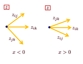
Figure 37: For the path of vacuum weights in Figure 38 we have BPS rays crossing as in the standard marginal stability analysis of the two-dimensional wall-crossing formula.

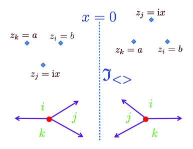
Figure 38: An example of a continuous path of vacuum weights crossing a wall of marginal stability. Here $z_{k}=a$ and $z_{i}=b$ with $a,b$ real and $a<0<b$. They do not depend on $x$, while $z_{j}(x)={\rm i}x$. We show typical vacuum weights for negative and positive $x$ and the associated trivalent vertex. As $x$ passes through zero the vertex degenerates with $z_{jk}(x)$ and $z_{ij}(x)$ becoming real. Note that with this path of weights the $\{i,j,k\}$ form a positive half-plane fan in the negative half-plane, while $\{k,j,i\}$ form a negative half-plane fan in the positive half-plane. If we choose $x_{\ell}<0<x_{r}$ there is an associated interface $\mathfrak{I}_{<>}$.

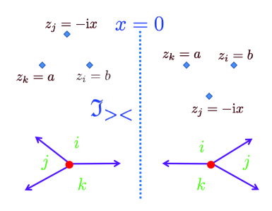
Figure 39: In this figure the path of weights shown in Figure 38 is reversed. Again, $z_{k}=a$ and $z_{i}=b$ with $a,b$ real and $a<0<b$, but now $z_{j}(x)=-{\rm i}x$. We show typical vacuum weights for negative and positive $x$ and the associated trivalent vertex. Note that with this path of weights the $\{i,j,k\}$ form a positive half-plane fan in the positive half-plane, while $\{k,j,i\}$ form a negative half-plane fan in the negative half-plane. In order to define an interface we choose initial and final points for the path $-x_{r}<0<-x_{\ell}$ so that, after translation, it can be composed with the path defining $\mathfrak{I}_{<>}$.

3.5 Categorified Wall-Crossing For 2d Solitons

The standard wall-crossing formula for BPS indices of 2d solitons was studied by Cecotti and Vafa in [2]. It is associated with a homotopy of vacuum weights so that the cyclic orders of the central charges gets reversed, as in Figure 37. We can realize this by the explicit homotopy of vacuum weights shown in Figures 38 and 39. The wall-crossing of the BPS indices is a special case of the famous Kontsevich-Soibelman wall-crossing formula:

$$(1+\mu_{ij}^{(1)}e_{ij})(1+\mu_{ik}^{(1)}e_{ik})(1+\mu_{jk}^{(1)}e_{jk})=(1+\mu_{jk}^{(2)}e_{jk})(1+\mu_{ik}^{(2)}e_{ik})(1+\mu_{ij}^{(2)}e_{ij})$$ (124)

which gives:

$$\begin{split}\mu_{ij}^{(2)}&=\mu_{ij}^{(1)}\\ \mu_{jk}^{(2)}&=\mu_{jk}^{(1)}\\ \mu_{ik}^{(2)}&=\mu_{ik}^{(1)}+\mu_{ij}^{(1)}\mu_{jk}^{(1)}.\\ \end{split}$$ (125)

To categorify this we seek to define Interfaces:

$$\mathfrak{I}_{<>}\in\mathfrak{B}\mathfrak{r}({\cal T}^{\ell},{\cal T}^{r})\qquad\qquad\&\qquad\qquad\mathfrak{I}_{><}\in\mathfrak{B}\mathfrak{r}({\cal T}^{r},{\cal T}^{\ell})$$ (126)

(where the notation is meant to remind us how the half-plane fans are configured in the negative and positive half-planes). Now, the essential statement constraining these Interfaces is that the composition of the Interfaces should be homotopy equivalent to the identity Interface:

$$\mathfrak{I}_{<>}\boxtimes\mathfrak{I}_{><}\sim\mathfrak{I}\mathfrak{d}_{{\cal T}^{\ell}}\qquad\qquad\&\qquad\qquad\mathfrak{I}_{><}\boxtimes\mathfrak{I}_{<>}\sim\mathfrak{I}\mathfrak{d}_{{\cal T}^{r}}.$$ (127)

In [9] we construct such Interfaces $\mathfrak{I}_{><}$ and $\mathfrak{I}_{<>}$ and show that the most natural solution to the constraints follows from:

$$\begin{split}R_{ij}^{(2)}&=R_{ij}^{(1)}\\ R_{jk}^{(2)}&=R_{jk}^{(1)}\\ R^{(2)}_{ik}-R^{(1)}_{ik}&=\left(R_{ij}\otimes R_{jk}\right)^{+}-\left(R_{ij}\otimes R_{jk}\right)^{-}\\ &=\left(R_{ij}^{+}-R_{ij}^{-}\right)\otimes\left(R_{jk}^{+}-R_{jk}^{-}\right)\\ \end{split}$$ (128)

where the superscript $\pm$ on the right hand side refers to the sign of $(-1)^{{\rm\textbf{F}}}$. We have written an identity of virtual vector spaces. One could move terms to left and right hand sides so that only plus signs appear and we would then have an identity of vector spaces. We have written the equation in terms of virtual vector spaces to bring out the fact that (128) is a categorification of the wall-crossing formulae (125).

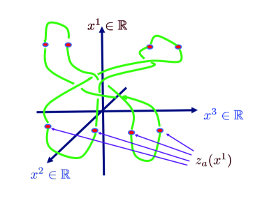
Figure 40: This figure depicts the a knot (actually, a link) in the boundary at $y=0$ at a fixed value of $x^{0}$. It is presented as a tangle evolving in the $x^{1}$ direction and therefore can be characterized as a trajectory of points $z_{a}(x^{1})$ in the complex $z=x^{2}+{\rm i}x^{3}$ plane. The tangle is closed by “creation” and “annihilation” of the points $z_{a}$ in pairs (with identical values of $k_{a}$).

3.6 Potential Application To Knot Homology

To conclude, let us consider very briefly the motivation from knot homology. For background see [18][19][20][7], and the review in §18.4 of [9]. The central idea is to consider five-dimensional supersymmetric gauge theory on a five-manifold with boundary:

$$M_{5}={\mathbb{R}}\times M_{3}\times{\mathbb{R}}_{+},$$ (129)

where $M_{3}$ is a three-manifold. The knot resides in $M_{3}$ on the boundary and is used to formulate the crucial boundary conditions for the instanton equations of the gauge theory. These 5d instanton equations were first written in [11, 18]. At a formal level they turn out to be the $\zeta$-instanton equations for a gauged Landau-Ginzburg model whose target space is a space of complexified gauge connections on $M_{3}$ [9]. In the case when $M_{3}={\mathbb{R}}\times C$, with $C$ a Riemann surface, the equations are also the $\zeta$-instanton equations for a gauged Landau-Ginzburg model whose target space is a space of complexified gauge fields on $\tilde{M}_{3}=C\times{\mathbb{R}}_{+}$. It is this latter form which forms the background for the discussion of [7]. In either case, the knot complex is the MSW complex for the Landau-Ginzburg theory.

When $M_{5}={\mathbb{R}}\times{\mathbb{R}}\times C\times{\mathbb{R}}_{+}$ we denote coordinates on the first two factors by $(x^{0},x^{1})$. We consider the case where the knot is in ${\mathbb{R}}^{3}$ (so $C$ is just the complex plane) and is furthermore presented as a tangle, i.e. an evolving set of points in the complex plane, $z_{a}(x^{1})$, $a=1,\dots n$, as in Figure 40.

For any collection $S$ of strands parallel to the $x^{1}$ axis

• Solutions of the 5d instanton equation which do not depend on $(x^{0},x^{1})$ will give some vacuum data ${\mathbb{V}}_{S}$.

• Solutions of the 5d instanton equation which depend only on the combination $x^{1}\cos\mu+x^{0}\sin\mu$ will provide the spaces of solitons which can interpolate between any two given vacua and thus web representations for the vacuum data ${\mathbb{V}}_{S}$.

• Solutions of the 5d instanton equation with fan-like asymptotics in the $(x^{0},x^{1})$ plane will provide interior amplitudes $\beta_{S}$ and thus Theories ${\cal T}_{S}$.

If $S$ is an empty collection, we expect the theory ${\cal T}_{S}$ to be trivial.

Similarly, for any “supersymmetric interface” ${{\cal I}}$, i.e. a time-independent boundary condition for the 5d equations which involves a set of parallel strands $S^{-}$ for $x^{1}\ll-L$ and a set of parallel strands $S^{+}$ for $x^{1}\gg L$

• Solutions of the 5d instanton equation which do not depend on time will give Chan-Paton data ${\cal E}^{{\cal I}}_{j,j^{\prime}}$.

• Solutions of the 5d instanton equation with fan-like asymptotics in the $(x^{0},x^{1})$ plane will provide boundary amplitudes ${\cal B}^{{\cal I}}$ and thus an Interface $\mathfrak{I}[{{\cal I}}]$ between Theories ${\cal T}_{S^{-}}$ and ${\cal T}_{S^{+}}$.

We can assume that the stretched link is approximated by a sequence of collections of strands $S_{a}$, starting and ending with the empty collection $S_{0}=S_{n}=0$, separated by interfaces ${{\cal I}}_{a,a+1}$. The approximate ground states and instantons of the knot homology complex will literally coincide with the chain complex of the Interface $\mathfrak{I}({\rm Link})$ between the trivial Theory and itself, defined as the composition of the Interfaces $\mathfrak{I}[{{\cal I}}_{a,a+1}]$

$$\mathfrak{I}({\rm Link}):=\mathfrak{I}[{{\cal I}}_{0,1}]\boxtimes\cdots\boxtimes\mathfrak{I}[{{\cal I}}_{n-1,n}].$$ (130)

Furthermore, if we allow the transverse position of the strands to evolve adiabatically in between discrete events such as recombination of strands, according to some profile $S_{a}(x^{1})$, we expect the knot homology complex to coincide with the chain complex of an Interface $\mathfrak{I}({\rm Link})$ which include the insertion of the corresponding categorical parallel transport Interfaces:

$$\mathfrak{I}({\rm Link}):=\mathfrak{I}[{{\cal I}}_{0,1}]\boxtimes\mathfrak{I}[{\cal T}_{S_{1}(x^{1})}]\boxtimes\cdots\boxtimes\mathfrak{I}[{\cal T}_{S_{n-1}(x^{1})}]\boxtimes\mathfrak{I}[{{\cal I}}_{n-1,n}].$$ (131)

We conjecture that the chain complexes so constructed define a knot homology theory. The required double-grading comes about as follows: The $R_{ij}$ and Chan-Paton data have the usual grading by F. The second grading comes from the fact that the relevant superpotential $W$ is a Chern-Simons functional. In particular, it is not single valued and $dW$ can have interesting periods.

References

- [1] S. M. Carroll, S. Hellerman and M. Trodden, “Domain wall junctions are 1/4 - BPS states,” Phys. Rev. D 61, 065001 (2000) [hep-th/9905217].
- [2] S. Cecotti, P. Fendley, K. A. Intriligator and C. Vafa, “A New supersymmetric index,” Nucl. Phys. B 386, 405 (1992) [hep-th/9204102].
- [3] S. Cecotti and C. Vafa, “On classification of supersymmetric theories,” Commun. Math. Phys. 158, 569 (1993) [hep-th/9211097].
- [4] F. Chapoton and M. Livernet, “Pre-Lie Algebras and the Rooted Trees Operad,” Intl. Math. Res. Notes, 2001, No.8
- [5] H. Fan, T. J. Jarvis and Y. Ruan, “The Witten equation, mirror symmetry and quantum singularity theory,” arXiv:0712.4021 [math.AG].
- [6] P. Fendley and K. A. Intriligator, “Scattering and thermodynamics in integrable N=2 theories,” Nucl. Phys. B 380, 265 (1992) [hep-th/9202011].
- [7] D. Gaiotto and E. Witten, “Knot Invariants from Four-Dimensional Gauge Theory,” arXiv:1106.4789 [hep-th].
- [8] D. Gaiotto, G. W. Moore and A. Neitzke, “Spectral networks,” arXiv:1204.4824 [hep-th].
- [9] D. Gaiotto, G. W. Moore and E. Witten, “Algebra of the Infrared: String Field Theoretic Structures in Massive Field Theory In Two Dimensions,” arXiv:1506.04087 [hep-th].
- [10] G. W. Gibbons and P. K. Townsend, “A Bogomolny equation for intersecting domain walls,” Phys. Rev. Lett. 83, 1727 (1999) [hep-th/9905196].
- [11] A. Haydys, “Seidel-Fukaya Category And Gauge Theory,” arXiv:1010.2353.
- [12] M. Kapranov, M. Kontsevich and Y. Soibelman, “Algebra of the infrared and secondary polytopes,” arXiv:1408.2673 [math.SG].
- [13] M. Kontsevich and Y. Soibelman, “Stability structures, motivic Donaldson-Thomas invariants and cluster transformations,” arXiv:0811.2435 [math.AG].
- [14] H. Oda, K. Ito, M. Naganuma and N. Sakai, “An Exact solution of BPS domain wall junction,” Phys. Lett. B 471, 140 (1999) doi:10.1016/S0370-2693(99)01355-6 [hep-th/9910095].
- [15] P. Seidel, Fukaya categories and Picard-Lefschetz theory, European Mathematical Society, Zürich, 2008
- [16] E. Witten, “Supersymmetry and Morse theory,” J. Diff. Geom. 17, 661 (1982).
- [17] E. Witten, “Algebraic geometry associated with matrix models of two-dimensional gravity,” in Topological methods in modern mathematics (Stony Brook, NY, 1991), Publish or Perish, Houston, TX, 1993, 235–269.
- [18] E. Witten, “Fivebranes and Knots,” arXiv:1101.3216 [hep-th].
- [19] E. Witten, “Khovanov Homology And Gauge Theory,” arXiv:1108.3103 [math.GT].
- [20] E. Witten, “Two Lectures On The Jones Polynomial And Khovanov Homology,” arXiv:1401.6996 [math.GT].