On nodal domains in Euclidean balls

Abstract.

Å. Pleijel (1956) has proved that in the case of the Laplacian with Dirichlet condition, the equality in the Courant nodal theorem (Courant sharp situation) can only be true for a finite number of eigenvalues when the dimension is $\geq 2$. Recently Polterovich extended the result to the Neumann problem in two dimensions in the case when the boundary is piecewise analytic. A question coming from the theory of spectral minimal partitions has motivated the analysis of the cases when one has equality in Courant’s theorem.

We identify the Courant sharp eigenvalues for the Dirichlet and the Neumann Laplacians in balls in $\mathbb{R}^{d}$, $d\geq 2$. It is the first result of this type holding in any dimension. The corresponding result for the Dirichlet Laplacian in the disc in $\mathbb{R}^{2}$ was obtained by B. Helffer, T. Hoffmann-Ostenhof and S. Terracini.

1. Introduction and main results

We consider the problem of counting nodal domains of eigenfunctions of the self-adjoint realization of the Laplacian, $-\Delta$ in the unit ball in $\mathbb{R}^{d}$. The “nodal domains” are the connected components of the zeroset of the eigenfunction in the ball. We consider the Dirichlet problem for $d\geq 3$ and the Neumann problem for $d\geq 2$ (the corresponding results for the Dirichlet problem for $d=2$ was given in [7]).

To be more precise, denoting by $\lambda_{n}$ the $n$th eigenvalue, our goal is to discuss the property of Courant sharpness of these operators, that is the existence of eigenvalues $\lambda_{n}$ for which there exists an eigenfunction with exactly $n$ nodal domains. We recall that Courant’s theorem says that the number of nodal domains, $\mu(\Psi)$, of an eigenfunction $\Psi$ corresponding to $\lambda_{n}$ is bounded by $n$. Moreover, it has been proven that the number of Courant sharp cases must be finite, see [17] for the Dirichlet case and [19] for the Neumann case (in dimension $2$ only and for piecewise analytic boundaries). The two first eigenvalues are always Courant sharp. We will prove the following.

Theorem 1.1.

The only Courant sharp eigenvalues for the Neumann Laplacian for the disc are $\lambda_{1}$, $\lambda_{2}$ and $\lambda_{4}$.

Theorem 1.2.

The only Courant sharp eigenvalues for the Dirichlet and Neumann Laplacians for the ball in $\mathbb{R}^{d}$, $d\geq 3$, are $\lambda_{1}$ and $\lambda_{2}$.

This analysis is motivated by the problem of spectral minimal $k$-partitions, where one is interested in minimizing $\max_{j}\lambda_{1}(D_{j})$ over the family $\mathcal{D}=(D_{1},\cdots,D_{k})$ of pairwise disjoint open sets in a domain $\Omega$, where $\lambda_{1}(D_{j})$ denotes either the Dirichlet ground state energy (if we analyze the Dirichlet spectral partitions of an open set $\Omega$) or the Dirichlet–Neumann ground state energy for the Laplacian in $D_{j}$ with Neumann condition on $\partial D_{j}\cap\partial\Omega$ and Dirichlet condition on the remaining part of $\partial D_{j}$. There are now many results in the two-dimensional (2D) case. We refer to [4] for a recent review. In higher dimensions much less is done, and we only know of the determination of all Courant sharp Dirichlet eigenvalues in the cube in three dimensions, [10]. We also know less about the properties of $k$-minimal partitions in higher dimensions. This will not create too much problems below, because we will work with explicit nodal domains of eigenfunctions, which in spherical coordinates will be expressed as a product of an interval (in the radial direction) by a nodal domain of a spherical harmonics in $\mathbb{S}^{d-1}$.

In Section 2 we recall how one describes the spectrum of the Laplace operator. As a part of the analysis of the Neumann problem, we use and extend a recent result on the zeros of derivatives of the Bessel functions $J_{\nu}$, saying that $J_{\nu}^{\prime}$ and $J_{\nu+p}^{\prime}$ have no common positive zeros if $\nu\geq 0$ and $p\geq 1$ are integers. This was proved by M. Ashu in his Bachelor thesis [2].

In Section 3 we discuss Courant sharpness. As a first result, we use a symmetry argument to extend a result by Leydold ([14, 15]) from $\mathbb{S}^{2}$ to $\mathbb{S}^{d-1}$, $d\geq 4$, saying that only the first two eigenvalues of the Laplace–Beltrami operator on $\mathbb{S}^{d-1}$ are Courant sharp. We then continue towards the proofs of the Theorems 1.1 and 1.2, by reducing the number of cases that need special treatment by using what we call a twisting trick. In short, it says that if the eigenfunction is non-radial, and if the eigenfunction is zero on a set $|x|=\rho$, $\rho<1$, then one can consider the same eigenfunction, but where one makes a small rotation of the inner ball $|x|<\rho$, breaking the necessary symmetry. We refer to Subsection 3.2 for the full details. This leaves two families of eigenfunctions to consider. In Subsection 3.3 we finish the proof of Theorem 1.2 in the case of Dirichlet boundary condition, by using an interlacing property of zeros of Bessel functions. In Subsection 3.4 we finish the proof of Theorem 1.1 and the Neumann part of Theorem 1.2. We remark that the proof of Theorem 1.1 is quite close to the proof of the Dirichlet case for the disc [7, Section 9].

In Section 4, we discuss the possible extension of a theorem by Å. Pleijel, [17]. The question is to determine if there exists a constant $\gamma<1$ such that, for any infinite sequence of eigenpairs $(\lambda_{n},u_{n})$

$$\lim\sup\frac{\mu(u_{n})}{n}\leq\gamma\,.$$

For the Dirichlet problem, this is indeed the case as proved in the paper of Bérard-Meyer [3], which establishes, in any dimension $d\geq 2$ for bounded open sets in $\mathbb{R}^{d}$ or $d$ dimensional compact Riemannian manifolds, the existence of an explicit universal constant $\gamma(d)<1$ (extending [16]). This was also solved previously for the Neumann problem in dimension 2 [19].

Finally, in Section 5, we establish new monotonicity properties of the function $\gamma(d)$.

Remark 1.3.

It would be interesting to consider the problem of minimal $k$-partitions of the ball in three dimensions. In the case $k=3$, it has been proved in [9] that the minimal $3$-partition of the sphere $\mathbb{S}^{2}$ is up to rotation determined by the intersection of $\mathbb{S}^{2}$ with three half-planes crossing along the vertical axis with equal angle $\frac{2\pi}{3}$. It is natural to conjecture that the minimal $3$-partition for the ball is up to rotation determined by the intersection of the ball with three half-planes crossing along the vertical axis with equal angle $\frac{2\pi}{3}$.

2. Spectrum of the Laplace operator in the unit ball in $\mathbb{R}^{d}$

We denote by $-\Delta^{D}$ and $-\Delta^{N}$ the Dirichlet and Neumann Laplace operators, respectively, in the unit ball in $\mathbb{R}^{d}$, $d\geq 2$. The Laplace operator $-\Delta$ can be written as

$$-\Delta=-\frac{\partial^{2}}{\partial r^{2}}-\frac{d-1}{r}\frac{\partial}{\partial r}+\frac{1}{r^{2}}(-\Delta_{\mathbb{S}^{d-1}}),$$

where $r=|x|$ is the radial variable and $\Delta_{\mathbb{S}^{d-1}}$ is the Laplace–Beltrami operator, acting in $L^{2}(\mathbb{S}^{d-1})$.

Proposition 2.1 ([21, Theorem 22.1 and Corollary 22.1]).

Assume that $d\geq 2$. The spectrum of $-\Delta_{\mathbb{S}^{d-1}}$ consists of eigenvalues

$$\ell(\ell+d-2),\quad\ell\in\mathbb{N}\,.$$

The multiplicity of the eigenvalue $\ell(\ell+d-2)$ is given by

$$\Lambda_{\ell,d}:=\binom{\ell+d-1}{d-1}-\binom{\ell+d-3}{d-1}\,,$$

which coincides with the dimension of the space of homogeneous, harmonic polynomials of degree $\ell$.

This leads us to consider the Dirichlet and Neumann eigenvalues of the ordinary differential operator

$$\mathcal{L}=-\frac{d^{2}}{dr^{2}}-\frac{d-1}{r}\frac{d}{dr}+\frac{\ell(\ell+d-2)}{r^{2}}\,,$$

acting in $L^{2}((0,1),r^{d-1}\,dr)\,$.
The general solution to $\mathcal{L}u=\lambda u$ is given by

$$u(r)=c_{1}r^{\frac{2-d}{2}}J_{\frac{1}{2}(2\ell+d-2)}(\sqrt{\lambda}r)+c_{2}r^{\frac{2-d}{2}}Y_{\frac{1}{2}(2\ell+d-2)}(\sqrt{\lambda}r)\,,$$

where $J_{\nu}$ and $Y_{\nu}$ denote the Bessel functions of order $\nu$, and of first and second kind, respectively. The Bessel functions of the second kind are too singular at the origin to be considered as eigenfunctions.

To state the next results, we introduce the function

$$\Xi_{\ell}^{(d)}(r)=r^{\frac{2-d}{2}}J_{\frac{1}{2}(2\ell+d-2)}(r)\,,$$

which is also denoted $\Xi_{\ell}$ for simplicity.

Proposition 2.2.

The spectrum of $-\Delta^{D}$ in the unit ball in $\mathbb{R}^{d}$, $d\geq 2$ , consists of eigenvalues

$$\lambda_{\ell,m}^{D}=\bigl{(}\alpha_{\ell,m}^{(d)}\bigr{)}^{2}\,,\quad\ell\in\mathbb{N}\,,\ m\in\mathbb{N}\setminus\{0\},$$

where $\alpha_{\ell,m}^{(d)}$ denotes the $m$th positive zero of the function $\Xi_{\ell}^{(d)}$. Each eigenvalue has multiplicity $\Lambda_{\ell,d}\,$.

Proposition 2.3.

The spectrum of $-\Delta^{N}$ in the unit ball in $\mathbb{R}^{d}$, $d\geq 2$ , consists of eigenvalues

$$\lambda_{\ell,m}^{N}=\bigl{(}\beta_{\ell,m}^{(d)}\bigr{)}^{2}\,,\quad\ell\in\mathbb{N}\,,\ m\in\mathbb{N}\setminus\{0\}\,,$$

where $\beta_{\ell,m}^{(d)}$ denotes the $m$th positive (non-negative if $\ell=0$) zero of the function $r\mapsto\frac{d}{dr}\Xi_{\ell}^{(d)}(r)$. Each eigenvalue has multiplicity $\Lambda_{\ell,d}\,$.

The only statement in these propositions that needs a proof is that of the multiplicity of the eigenvalues. For the Dirichlet case the needed result is given in [25, §15.28]. It says that the Bessel functions $J_{\nu}$ and $J_{\nu+p}$ do not have any common positive zeros. This was conjectured by Bourget (1866), and follows from a deep result obtained by Siegel [22] in 1929. He proved that if $r>0$ is an algebraic number, and $\nu\in\mathbb{Q}$, then $J_{\nu}(r)$ is not an algebraic number.

The corresponding result for the Neumann problem was solved recently in the case $d=2$ in Ashu’s Bachelor thesis, [2]. In this particular case the statement is that $J_{\nu}^{\prime}$ and $J_{\nu+p}^{\prime}$ have no common positive zeros. Again, there is a deep result behind, given in [20, page 217], which we will come back to in the proof of the first lemma below.

Lemma 2.4.

Assume that $d\geq 2$ and that $\ell\in\mathbb{N}$. Then the positive zeros of the function $\Xi_{\ell}^{(d)}$ are transcendental numbers.

Proof.

The functions $K_{\nu}$ (not to be mixed up with the modified Bessel functions) are introduced in [20] via the identity

$$J_{\nu}(r)=\frac{1}{\Gamma(\nu+1)}\Bigl{(}\frac{r}{2}\Bigr{)}^{\nu}K_{\nu}(r)\,.$$

We express the derivative of $\Xi_{\ell}^{(d)}$ in terms of these $K$ functions,

$$\frac{d}{dr}\Xi_{\ell}^{(d)}(r)=r^{-d/2}\frac{1}{\Gamma(\ell+d/2)}\Bigl{(}\frac{r}{2}\Bigr{)}^{\ell+d/2-1}\biggl{[}\ell K_{\ell+d/2-1}(r)+rK_{\ell+d/2-1}^{\prime}(r)\biggr{]}\,.$$ (2.1)

Assume that $r>0$ is an algebraic zero of $r\mapsto\frac{d}{dr}\Xi_{\ell}^{(d)}(r)$. Then both $K_{\ell+d/2-1}(r)$ and $K_{\ell+d/2-1}^{\prime}(r)$ are transcendental according to [20, Theorem 6.3]. In particular they are non-zero. However, as noted in [20, page 217], also $K_{\ell+d/2-1}^{\prime}(r)/K_{\ell+d/2-1}(r)$ is transcendental. But then $\ell/r$ is transcendental by (2.1). Since $\ell$ is an integer and $r$ was assumed to be algebraic, this is a contradiction. ∎

Proposition 2.3 is a direct consequence of this lemma.

Lemma 2.5.

Assume that $d\geq 2$, $\ell\in\mathbb{N}$ and $p\in\mathbb{N}\setminus\{0\}$. Then the functions $r\mapsto\frac{d}{dr}\Xi_{\ell}^{(d)}$ and $r\mapsto\frac{d}{dr}\Xi_{\ell+p}^{(d)}$ have no common positive zeros.

Before giving the proof, we recall some recursion formulas for the Bessel functions, valid for all $\nu\in\mathbb{R}$ and positive $r$,

$$J_{\nu}^{\prime}(r) =\frac{\nu}{r}J_{\nu}(r)-J_{\nu+1}(r)\,,$$ (2.2)

$$J_{\nu}^{\prime}(r) =-\frac{\nu}{r}J_{\nu}(r)+J_{\nu-1}(r)\,,$$ (2.3)

$$J_{\nu+1}(r) =\frac{2\nu}{r}J_{\nu}(r)-J_{\nu-1}(r)\,.$$ (2.4)

Proof of Lemma 2.5.

By (2.2)–(2.4), we get the corresponding formulas for $\Xi_{\ell}\,$,

$$\Xi_{\ell}^{\prime}(r) =\frac{\ell}{r}\Xi_{\ell}(r)-\Xi_{\ell+1}(r)\,,\quad\ell\geq 0\,,$$ (2.5)

$$\Xi_{\ell}^{\prime}(r) =-\frac{\ell+d-2}{r}\Xi_{\ell}(r)+\Xi_{\ell-1}(r)\,,\quad\ell\geq 1\,,$$ (2.6)

$$\Xi_{\ell}(r) =\frac{2\ell+d-4}{r}\Xi_{\ell-1}(r)-\Xi_{\ell-2}(r)\,,\quad\ell\geq 2\,.$$ (2.7)

We divide the proof into different cases, and do the proof by contradiction, using recursion formulas and Lemma 2.4.

Case 1, $\ell=0$ and $p=1\,$:

If, for $r>0$, $\Xi_{0}^{\prime}(r)=\Xi_{1}^{\prime}(r)=0\,$, then (2.5) with $\ell=0$ implies that $\Xi_{1}(r)=0\,$, which contradicts Cauchy uniqueness.

Case 2, $\ell=0$ and $p\geq 2\,$:

Assume that $r>0$ is a zero of $\Xi_{0}^{\prime}$ and $\Xi_{p}^{\prime}\,$. As in Case 1, we find that $\Xi_{1}(r)=0$, and so by (2.7), $\Xi_{2}(r)=-\Xi_{0}(r)\,$. One application of (2.6) gives

$$0=\Xi_{p}^{\prime}(r)=-\frac{p+d-2}{r}\,\Xi_{p}(r)+\Xi_{p-1}(r)\,.$$

Next, we use (2.7) several times to reduce the right-hand side to an expression involving $\Xi_{2}(r)$ and $\Xi_{1}(r)$ only. After $p-2$ applications we find a polynomial $Q$ in the variable $1/r$ times $\Xi_{2}(r)$ only, since $\Xi_{1}(r)=0\,$. The highest degree term of the polynomial is

$$-\frac{p+d-2}{r}\,\frac{2p+d-4}{r}\,\frac{2p+d-6}{r}\cdots\frac{2p+d-(2p-2)}{r}\,.$$

Since $\Xi_{2}(r)=-\Xi_{0}(r)\,$, we find that

$$0=Q(1/r)\Xi_{0}(r)\,,$$

where $Q$ is a non-vanishing polynomial with rational coefficients. Since $r$ is transcendental by Lemma 2.4, $Q(1/r)\neq 0\,$. But $\Xi_{0}(r)\neq 0$ by Cauchy uniqueness, so we end up at a contradiction and conclude that $\Xi_{0}^{\prime}$ and $\Xi_{p}^{\prime}$ have no common positive zero.

Case 3, $\ell\geq 1$ and $p\geq 1\,$:

Again, assume that $r>0$ is a zero of $\Xi_{\ell}^{\prime}$ and $\Xi_{\ell+p}^{\prime}\,$. This means, using (2.5) and (2.6) respectively,

$$0 =\Xi_{\ell}^{\prime}(r)=-\Xi_{\ell+1}(r)+\frac{\ell}{r}\Xi_{\ell}(r)\,,$$ (2.8)

$$0 =\Xi_{\ell+p}^{\prime}(r)=-\frac{\ell+p+d-2}{r}\Xi_{\ell+p}(r)+\Xi_{\ell+p-1}(r)\,.$$

We use (2.7) repeatedly, to reduce the second equation so that it involves only $\Xi_{\ell}(r)$ and $\Xi_{\ell+1}(r)$, with polynomial (in the variable $1/r$) coefficients in front. The highest degree (in $1/r$) coefficient in front of $\Xi_{\ell+1}(r)$ will, after $p-1$ steps, become

$$-\frac{\ell+p+d-2}{r}\frac{2\ell+2p+d-4}{r}\frac{2\ell+2p+d-6}{r}\cdots\frac{2\ell+2p+d-2p}{r}\,,$$

and once reduced, while calculating the determinant of the resulting system, this term will be multiplied with $\ell/r$ (that is in front of $\Xi_{\ell}(r)$ in (2.8)), which will higher its degree (in $1/r$) by one. No such term can occur elsewhere, and thus for the determinant of the system to be zero, $r$ must solve a polynomial equation with rational coefficients, so $r$ is algebraic. That contradicts Lemma 2.4. The other possibility is that $\Xi_{\ell}(r)=\Xi_{\ell+1}(r)=0\,$. But that would imply that $\Xi_{\ell}(r)=\Xi_{\ell}^{\prime}(r)=0\,$, which, again, contradicts the Cauchy uniqueness. ∎

3. Courant sharpness

3.1. The result on $\mathbb{S}^{d-1}$

We first analyze the case of the sphere and extends Leydold’s result to $\mathbb{S}^{d-1}$ for $d\geq 3$.

Theorem 3.1.

If $d\geq 3$, the only Courant sharp cases for the Laplace–Beltrami operator on $\mathbb{S}^{d-1}$ correspond to the two first eigenvalues.

In the proof we need the following version of Courant’s theorem with symmetry (see for example [4, Subsection 2.4]) which we also prove for the sake of completeness.

Theorem 3.2.

Given an eigenfunction which is symmetric or antisymmetric with respect to the antipodal map, the number of its nodal domains is not greater than two times the smallest labeling of the corresponding eigenvalue inside its symmetry space.

Proof.

We note that each eigenspace has a specific symmetry with respect to the antipodal map. An eigenfunction $\psi_{\ell}$ associated with the eigenvalue $\ell(\ell+d-2)$ satisfies indeed

$$\psi_{\ell}(-\omega)=(-1)^{\ell}\psi_{\ell}(\omega)\,,\quad\forall\omega\in\mathbb{S}^{d-1}\,.$$

This is an immediate consequence of the fact that $\psi_{\ell}$ is the restriction to $\mathbb{S}^{d-1}$ of an homogeneous polynomial of degree $\ell$ of $d$ variables.

With this in mind, we first assume that $\ell$ is odd, and hence let $\psi_{\ell}$ be an eigenfunction with minimal labeling $\nu$ inside the antisymmetric space. Let us assume, to get a contradiction, that

$$\mu(\psi_{\ell})\geq 2\nu+1\,.$$

We note that by antisymmetry, $\mu(\psi_{\ell})$ is even. Hence we would have actually

$$\mu(\psi_{\ell})\geq 2\nu+2\,.$$

We now follow the standard proof of Courant’s theorem. Selecting $(\mu(\psi_{\ell})/2\,-1)$ pairs of symmetric nodal domains, we can construct an antisymmetric function, which is orthogonal to the antisymmetric eigenspace corresponding to the $\nu-1$ first eigenvalues and has an energy not greater than the $\nu$-th eigenvalue. Using the mini-max characterization of the $\nu$:th eigenvalue, we get that this function is an antisymmetric eigenfunction which vanishes in the two remaining nodal domains. This gives the contradiction using the unique continuation principle.

Next, assume that $\ell$ is even and that $\psi_{\ell}$ is an eigenfunction with minimal labeling $\nu$ inside the symmetric space. We assume, again to get a contradiction, that

$$\mu(\psi_{\ell})\geq 2\nu+1\,.$$

We have

$$\mu(\psi_{\ell})=\mu^{\prime}+2\mu^{\prime\prime}$$

where $\mu^{\prime}$ is the number of nodal domains which are symmetric and $\mu^{\prime\prime}$ is the number of pairs of nodal domains which are exchanged by symmetry.

If $\mu^{\prime}=0$, the proof is identical to the antisymmetric one. If $\mu^{\prime}\geq 1$, we can select $\mu^{\prime}-1$ symmetric nodal domains and $\mu^{\prime\prime}$ pairs of nodal domains exchanged by symmetry and construct a symmetric function which is orthogonal to the symmetric eigenspace corresponding to the $\nu-1$ first eigenvalues and has an energy not greater than the $\nu$:th eigenvalue. Here we have used our assumption by contradiction to get that $\mu^{\prime}-1+2\mu^{\prime\prime}\geq\nu$. We get a contradiction just as before. ∎

Proof of Theorem 3.1.

This is just an adaptation of Leydold’s proof ([14, 15]).

We consider the (smallest) labeling of the eigenvalue $\ell(\ell+d-2)$, i.e. the smallest $n$ such that $\lambda_{n}=\ell(\ell+d-2)$. According to Proposition 2.1, the smallest labeling of the eigenvalue $\ell(\ell+d-2)$ is obtained by $1$ if $\ell=0$, $2$ if $\ell=1$, and

$$1+\binom{\ell+d-2}{d-1}+\binom{\ell+d-3}{d-1}\,,\quad\forall\ell\geq 2\,.$$

Using Theorem 3.2 on the eigenvalue $\ell(\ell+d-2)$, we get

$$\mu(u_{\ell})\leq 2\biggl{[}\binom{\ell+d-3}{d-1}+1\biggr{]}\,.$$

To compute this labeling we have used that for a given $\ell$, the labeling is obtained by adding $1$ to the sum of the multiplicity associated with the $\ell^{\prime}<\ell$ with the same parity as $\ell$.

Hence, we have to check that if $\ell\geq 2$ and $d\geq 3\,$, then

$$2\biggl{[}\binom{\ell+d-3}{d-1}+1\biggr{]}<1+\binom{\ell+d-2}{d-1}+\binom{\ell+d-3}{d-1}\,.$$ (3.1)

Since $\binom{\ell+d-2}{d-1}=\binom{\ell+d-3}{d-2}+\binom{\ell+d-3}{d-1}\,$, the inequality (3.1) reads $1<\binom{\ell+d-3}{d-2}\,$, which is satisfied when $\ell\geq 2$ and $d\geq 3\,$. ∎

3.2. Twisting trick

Lemma 3.3.

If $\ell\geq 1$ and $m\geq 2$ then neither $\lambda_{\ell,m}^{D}$ nor $\lambda_{\ell,m}^{N}$ can be Courant sharp.

Because the theory of minimal partitions has not been developed to the same extend when $d>3$, we explain how the proof goes, without referring to [7, 8] which are mainly devoted to the case when the dimension is 2 or 3. The proof below is somewhat reminiscent of a proof written in collaboration with T. Hoffmann-Ostenhof (2005), which was never published but is mentioned in [7].

Proof.

We start with the Dirichlet situation, and omit the $D$ in the notation. All eigenvalues occurring are Dirichlet eigenvalues of the Laplace operator. The domain will differ, and we will be explicit about that.

Assume that we have a Courant sharp eigenvalue $\lambda_{n}=\lambda_{\ell,m}\,$, with $\ell\geq 1$ and $m\geq 2$. We will construct a partition $\widehat{\mathcal{D}}$ of $n$ non-intersecting open sets $\{\widehat{D}_{j}\}_{j=1}^{n}$ in the ball, such that

$$\max_{j}\lambda_{1}(\widehat{D}_{j})<\lambda_{n}\,.$$

This leads to a contradiction by the minimax characterization of the $n$th eigenvalue.

Since we assume that $\lambda_{n}$ is Courant sharp, there exists an eigenfunction $\Psi$ having exactly $n$ nodal components. Moreover, this $\Psi$ cannot be radial (since $\ell\geq 1$). So we have $\Psi(r,\omega)=u_{\ell,m}(r)\psi_{\ell}(\omega)$ where $\psi_{\ell}$ is a spherical harmonic. We let $\rho_{1}$ be the first zero of $u_{\ell,m}$ in $(0,1)$ (which exists since $m\geq 2$) and $\rho_{2}$ be the second zero, if it exists, and $\rho_{2}=1$ otherwise. The ball is naturally divided into the parts $|x|<\rho_{1}$ and $\rho_{1}<|x|<1$. Next, we define the function $\widetilde{\Psi}$ as

$$\widetilde{\Psi}(x)=\begin{cases}\Psi(\mathsf{R}x),&|x|<\rho_{1}\,,\\ \Psi(x),&\rho_{1}<|x|<1\,.\end{cases}$$

Here $\mathsf{R}$ is a small rotation, constructed in such a way that the symmetry is broken.

Let us denote by $\widetilde{\mathcal{D}}=\bigcup_{j=1}^{n}\widetilde{D}_{j}$ the twisted partition of nodal domains corresponding to $\widetilde{\Psi}$.

We now consider a pair of nodal domains of $\Psi$ in the form (after relabeling) $D_{1}:=(0,\rho_{1})\times\Omega$ and $D_{2}:=(\rho_{1},\rho_{2})\times\Omega$. The twisting leads to the pair (see Figure 3.1, middle subfigure) $\widetilde{D}_{1}:=(0,\rho_{1})\times\mathsf{R}\Omega$ and $\widetilde{D}_{2}=D_{2}:=(\rho_{1},\rho_{2})\times\Omega$. Their boundary is $\{\rho_{1}\}\times(\Omega\cap\mathsf{R}\Omega)$. The sets $\widetilde{D}_{1}$ and $\widetilde{D}_{2}$ cannot be the $2$-partition of a second eigenfunction in $\widetilde{D}_{1,2}:=\operatorname{Int}\Bigl{(}\overline{\widetilde{D}_{1}}\cup\overline{\widetilde{D}_{2}}\Bigr{)}$. If it was true, it would exist $\mu\in\mathbb{R}$ such that $\mu\psi_{\ell}=\psi_{\ell}\circ\mathsf{R}$ in $\Omega\cap\mathsf{R}\Omega$. But this will imply $\mu\psi_{\ell}=\psi_{\ell}\circ\mathsf{R}$ on $\mathbb{S}^{d-1}$ by analyticity. We get a contradiction at the boundary of $\Omega$ or of $\mathsf{R}^{-1}\Omega$.

Thus, $\lambda_{2}(\widetilde{D}_{1,2})<\lambda_{n}$. By looking at the nodal set of a second eigenfunction $u_{1,2}$ in $\widetilde{D}_{1,2}$, we get two new sets $D_{1}^{\prime}$ and $D_{2}^{\prime}$ (the two nodal domains of $u_{1,2}$) such that

$$\lambda_{1}(D_{1}^{\prime})=\lambda_{1}(D_{2}^{\prime})<\lambda_{n}\,.$$

We recall that the remaining $n-2$ components of the partition $\widetilde{\mathcal{D}}$ have ground state energy $\lambda_{n}\,$. This is illustrated in Figure 3.1, to the right. If $n=2$, then we are done. Below we assume that $n>2$.

We continue, by considering $D_{1}^{\prime}$ or $D_{2}^{\prime}$, and one of its neighbors, having a boundary in common. Let us, for a while, denote this pair by $D_{1}^{\prime\prime}$ and $D_{2}^{\prime\prime}$. It is possible, using the Hadamard formula (see [12]) to change the common boundary of $D_{1}^{\prime\prime}$ and $D_{2}^{\prime\prime}$ in such a way that two new domains $\widetilde{D}_{1}^{\prime\prime}$ and $\widetilde{D}_{2}^{\prime\prime}$ are constructed, with

$$\lambda_{1}(D_{1}^{\prime\prime})<\lambda_{1}(\widetilde{D}_{1}^{\prime\prime})\leq\lambda_{1}(\widetilde{D}_{2}^{\prime\prime})<\lambda_{1}(D_{2}^{\prime\prime})\,.$$

In particular,

$$\max\Bigl{(}\lambda_{1}(\widetilde{D}_{1}^{\prime\prime}),\lambda_{1}(\widetilde{D}_{2}^{\prime\prime})\Bigr{)}<\max\Bigl{(}\lambda_{1}(D_{1}^{\prime\prime}),\lambda_{1}(D_{2}^{\prime\prime})\Bigr{)}=\lambda_{n}\,.$$

At this point we have constructed three domains inside the ball, with ground state energy strictly less than $\lambda_{n}$. If $n=3$, we are done. If $n\geq 4$, we continue this procedure recursively until all the remaining domains in the partition $\widetilde{\mathcal{D}}$ have been modified, and find in the end a new partition $\widehat{\mathcal{D}}$ of the ball, consisting of $n$ pairwise disjoint sets $\widehat{D}_{j}$, such that $\lambda_{1}(\widehat{D}_{j})<\lambda_{n}$ for all $j$.

The proof in the Neumann case is unchanged. One can do the necessary deformations in the boundaries where the Dirichlet condition is imposed. ∎

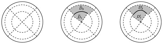
Figure 3.1. Twist showcase. The inner dashed circle correspond to $|x|=\rho_{1}\,$, and the outer one to $|x|=\rho_{2}\,$. Left: The partition of nodal domains of $\Psi$. Middle: The nodal partition of $\widetilde{\Psi}\,$. The common boundary of $\widetilde{D}_{1}$ and $\widetilde{D_{2}}$ is marked thicker. Right: The two nodal domains $D_{1}^{\prime}$ and $D_{2}^{\prime}$ of the second eigenfunction in $\widetilde{D}_{1,2}\,$.

Remark 3.4.

The proof of Lemma 3.3 is easier in dimension two, since we can refer to the “equal angle meeting” property, which is satisfied by any regular minimal partition as established in [7].

3.3. Remaining eigenvalues, Dirichlet case

Lemma 3.5.

Let $d\geq 3\,$. Then

$$\lambda_{1,1}^{D}<\lambda_{0,2}^{D}\,.$$

Proof.

Denote by $j_{\nu,m}$ the $m$th positive zero of the Bessel function $J_{\nu}\,$. The interlacing of zeros of $J_{\nu}$ (see [25, §15.22]),

$$0<j_{\nu,1}<j_{\nu+1,1}<j_{\nu,2}<j_{\nu+1,2}<j_{\nu,3}<\cdots\quad\forall\nu>-1\,,$$

implies, with $\nu=d/2\,$, that $\alpha_{1,1}<\alpha_{0,2}\,$, and so $\lambda_{1,1}^{D}<\lambda_{0,2}^{D}\,$. ∎

Hence only $\lambda_{0,1}^{D}$ can be (and is!) Courant sharp in the list $\lambda_{0,m}^{D}$. For the sequence $\lambda_{\ell,1}^{D}\,$, one can use what we have proven for the sphere. Only $\lambda_{0,1}^{D}$ and $\lambda_{1,1}^{D}$ can be Courant sharp. This completes the proof of Theorem 1.2 for the Dirichlet problem.

3.4. Remaining eigenvalues, Neumann case

Lemma 3.6.

Let $d\geq 2\,$. Then

$$\lambda_{1,1}^{N}<\lambda_{0,2}^{N}\,.$$

Proof.

We show that $\beta_{1,1}<\beta_{0,2}\,$. We recall that $\beta_{1,1}$ is the first positive zero of $\Xi_{1}^{\prime}$ and $\beta_{0,2}$ is the first positive zero of $\Xi_{0}^{\prime}$. But, according to (2.5), $\Xi_{0}^{\prime}(r)=-\Xi_{1}(r)$. Now, $\Xi_{1}(r)=2^{-d/2}/\Gamma(d/2+1)r+\mathcal{O}(r^{3})$ as $r\to 0$, so, in particular $\Xi_{1}(0)=0$ for all $d\geq 2$. It follows that $\beta_{1,1}<\beta_{0,2}$ by the mean value theorem. ∎

As a result, $\lambda_{0,m}^{N}$ cannot be Courant sharp if $m\geq 2\,$. Indeed, since the eigenfunctions corresponding to $\lambda_{0,m}^{N}$ have precisely $m$ nodal domains, and the labeling of $\lambda_{0,m}^{N}$ is at least $m+1$ because $\lambda_{0,1}^{N}<\lambda_{1,1}^{N}<\lambda_{0,2}^{N}\,$.

We continue with the eigenvalues $\lambda_{\ell,1}^{N}\,$, and start with the case $d=2$. We first see the following ordering for the eight first eigenvalues (see Figure 3.2):

$$\lambda_{1}^{N}=\lambda_{0,1}^{N}<\lambda_{2}^{N}=\lambda_{1,1}^{N}=\lambda_{3}^{N}<\lambda_{4}^{N}=\lambda_{2,1}^{N}=\lambda_{5}^{N}<\lambda_{6}^{N}=\lambda_{0,2}^{N}<\lambda_{7}^{N}=\lambda_{3,1}^{N}=\lambda_{8}^{N}\,,\,\ldots$$

with corresponding number of nodal domains

$$\mu_{1}=1\,,\,\mu_{2}=2\,,\,\mu_{4}=4\,,\,\mu_{6}=2\,,\,\mu_{7}=6\,,\ldots$$

We observe that $\lambda_{0,2}^{N}<\lambda_{3,1}^{N}\,$. Hence $\lambda_{\ell,1}^{N}$ cannot have a label lower than $2\ell+1$ in the complete ordered list of eigenvalues and the corresponding eigenfunction has exactly $2\ell$ nodal domains.

For $d\geq 3$ we can again use Theorem 3.1 to conclude that only the two first eigenvalues $\lambda_{0,1}^{N}$ and $\lambda_{1,1}^{N}$ can be Courant sharp.

This finishes the proof of Theorem 1.2 in the Neumann case.

Figure 3.2. Nodal domains for the eigenfunctions in the Neumann case for $d=2$. Thicker: The Courant sharp cases. The twisting argument excludes every case except $m=1$ (row one) and $\ell=0$ (column one) from being Courant sharp.

4. On Pleijel’s Theorem

We will discuss (the dimension-dependent) Pleijel constant

$$\gamma(d):=C_{d}^{-1}\,\bigl{(}\lambda_{1}(\mathbb{B}_{1}^{d})\bigr{)}^{-d/2}<1\,,$$

where $C_{d}$ is the Weyl constant $C_{d}:=(2\pi)^{-d}\omega_{d}$, $\omega_{d}$ is the volume of the unit ball in $\mathbb{R}^{d}$, and $\lambda_{1}(\mathbb{B}_{1}^{d})$ is the Dirichlet ground state energy of the Laplacian in the ball $\mathbb{B}_{1}^{d}$ of volume $1$. More explicitly, we get (see [3, Lemma 9])

$$\gamma(d)=\frac{2^{d-2}d^{2}\Gamma(d/2)^{2}}{(j_{\frac{d-2}{2},1})^{d}}\,.$$

As explained in the introduction, we focus on the Neumann case.

Theorem 4.1.

For any infinite sequence of eigenpairs $(\lambda_{n},u_{n})$ of the Neumann Laplacian in the unit ball in $\mathbb{R}^{d}$ ($d\geq 3$),

$$\lim\sup\frac{\mu(u_{n})}{n}\leq\gamma(d-1)<1\,.$$

We recall that $\gamma(2)=4/(j_{0,1}^{2})$ and that $\gamma(3)=\frac{9}{2\pi^{2}}$ (see [10]). We refer the reader to the last section for further properties of $\gamma(d)$. The Neumann case is more delicate but can result for the disc of the general result of Polterovich for domains in $\mathbb{R}^{2}$ with piecewise analytic boundary. In [19] he shows that Pleijel’s theorem holds with the same constant as for Dirichlet, as a consequence of a fine result due to Toth–Zelditch [24] on the relatively small number of points at the intersection of the boundary and the zeroset. To our knowledge, nothing has been established in dimension $d\geq 3$ for the Neumann problem.

A natural idea is to try to control the number of nodal domains touching the boundary on a set with non empty interior. This was the strategy proposed by Pleijel [17] for the square and more generally by I. Polterovich [19] for the $2D$-case. We know indeed that it is $\mu(\psi_{\ell})$ when the eigenfunction is $\Psi_{\ell,m}$. Hence the quotient between the number of “boundary” nodal sets divided by the total number tends to $0$, as $m\to+\infty$, like $\mathcal{O}(1/m)$. In this case, the “Faber–Krahn” proof works like in the Dirichlet case.

Hence it remains to control the case when $m\leq m_{0}$. In this case, $\ell$ tends to $+\infty$ as $\lambda^{N}_{\ell,m}\to+\infty$.

We know that the labeling of $\lambda_{\ell,m}^{N}$ is larger than $m\times n_{\ell}$ where $n_{\ell}$ is the labeling of $\ell(\ell+1)$. Hence we get

$$\lim\sup\frac{\mu(\Psi_{\ell,m})}{n_{\ell,m}}\leq\lim\sup\frac{\mu(\psi_{\ell})}{n_{\ell}}\leq\gamma(d-1)\,,$$

where $n_{\ell,m}$ (resp. $n_{\ell}$) is the labeling of $\lambda_{\ell,m}^{N}$ for the Laplacian in the ball (resp. of $\ell(\ell+1)$ for the Laplacian on the sphere). For the last inequality, we have used Bérard-Meyer (Pleijel like) theorem for the sphere $\mathbb{S}^{d-1}$. At this stage, we have obtained

$$\lim\sup\frac{\mu(u_{n})}{n}\leq\max\bigl{(}\gamma(d),\gamma(d-1)\bigr{)}<1\,.$$

The conclusion of the theorem is obtained using the monotonicity of $\gamma$ which will be established in the next section.

5. Monotonicity of $\gamma(d)$

We recall from [3, Lemma 9] that $\gamma(d)<1$. The proof of this inequality relies on the estimate

$$\Gamma(x)\leq x^{x-\frac{1}{2}}\,e^{-x}\,\sqrt{2\pi}\,e^{\frac{1}{12x}}\,,$$

which gives the estimate for $d\geq 18$ and of numerical computations (see below) for $d<18$. It is natural to discuss about the monotonicity of $d\mapsto\gamma(d)$.

Table 5.1. Table of values of $\displaystyle\gamma(d)$

$d$	2	3	4	5	6
$\gamma(d)$	0.691660	0.455945	0.296901	0.192940	0.125581
$d$	7	8	9	10	11
$\gamma(d)$	0.081982	0.053704	0.035306	0.023291	0.015417
$d$	12	13	14	15	16
$\gamma(d)$	0.010236	0.006817	0.004553	0.003048	0.002046
$d$	17	18	19	20	21
$\gamma(d)$	0.001376	0.000928	0.000627	0.000424	0.000288

Theorem 5.1.

The function $d\mapsto\gamma(d)$ is monotonically decreasing.

Proof.

We first recall that

Lemma 5.2.

$x\mapsto\Gamma(x)$ is logarithmically convex.

We write

$$\Gamma\Bigl{(}\frac{d}{2}+\frac{1}{2}\Bigr{)}/\Gamma\Bigl{(}\frac{d}{2}\Bigr{)}=\frac{1}{2}\,(d-1)\,\Gamma\Bigl{(}\frac{d}{2}-\frac{1}{2}\Bigr{)}/\Gamma\Bigl{(}\frac{d}{2}\Bigr{)}\,.$$

and use the logarithmic convexity of the $\Gamma$-function,

$$\Gamma\Bigl{(}\frac{d}{2}-\frac{1}{2}\Bigr{)}\leq\sqrt{\Gamma\Bigl{(}\frac{d}{2}-1\Bigr{)}}\sqrt{\Gamma\Bigl{(}\frac{d}{2}\Bigr{)}}\,.$$

This implies

$$\Gamma\Bigl{(}\frac{d}{2}-\frac{1}{2}\Bigr{)}/\Gamma\Bigl{(}\frac{d}{2}\Bigr{)}\leq\sqrt{\Gamma\Bigl{(}\frac{d}{2}-1\Bigr{)}/\Gamma\Bigl{(}\frac{d}{2}\Bigr{)}}=\frac{1}{\sqrt{\frac{d}{2}-1}}\,.$$

Finally, we deduce:

$$\biggl{[}\Gamma\Bigl{(}\frac{d}{2}+\frac{1}{2}\Bigr{)}/\Gamma\Bigl{(}\frac{d}{2}\Bigr{)}\biggr{]}^{2}\leq\frac{(d-1)^{2}}{2(d-2)}\,.$$ (5.1)

We next estimate $j_{d/2-1,1}/j_{d/2-1/2,1}$.

A less known result by Lewis–Muldoon is

Lemma 5.3 ([13, Formula (1.2)]).

For $\nu\geq 3$, $\nu\mapsto j_{\nu,1}^{2}$ is convex.

We write the convexity of $j_{\nu,1}^{2}$ (for $\nu\geq 3$)

$$j_{\nu-1,1}^{2}\leq\frac{1}{2}\bigl{(}j_{\nu-3/2,1}^{2}+j_{\nu-1/2,1}^{2}\bigr{)}\,.$$

This gives

$$\frac{j_{\nu-1,1}^{2}}{j_{\nu-1/2,1}^{2}}\leq\frac{1}{2}\biggl{(}\frac{j_{\nu-3/2,1}^{2}}{j_{\nu-1/2,1}^{2}}+1\biggr{)}\,.$$ (5.2)

In [1], Ashbaugh and Benguria prove:

$$\frac{d}{d+4}<\frac{(j_{d/2-1,1})^{2}}{(j_{d/2,1})^{2}}\leq\frac{\lambda_{1}(\Omega)}{\lambda_{2}(\Omega)},$$

where $\Omega$ is a $d$-dimensional domain, the right hand side inequality being attained for the ball and the left hand side being the Thomson inequality. In particular, for the $d$-cube, $\lambda_{1}(\Omega)=d$ and $\lambda_{2}(\Omega)=d+3$. This implies that

$$\frac{j_{d/2-1,1}}{j_{d/2,1}}\leq\Bigl{(}1-\frac{3}{d+3}\Bigr{)}^{1/2}\,.$$ (5.3)

To estimate the right hand side of (5.2), we use (5.3) (with $d$ replaced by $d-1$) to obtain

$$\frac{j_{d/2-1,1}^{2}}{j_{d/2-1/2,1}^{2}}\leq\frac{1}{2}\biggl{(}\frac{j_{(d-1)/2-1,1}^{2}}{j_{(d-1)/2,1}^{2}}+1\biggr{)}\leq 1-\frac{3}{2(d+2)}\,.$$ (5.4)

To our knowledge the best estimates for the zeros of Bessel functions are

$$\sqrt{\nu(\nu+2)}<j_{\nu,1}<\sqrt{\nu+1}\,\bigl{(}\sqrt{\nu+2}+1\bigr{)}\,.$$ (5.5)

The left estimate is available in Watson [25], the right one was proven by Chambers [5], by choosing a good trial state for the Rayleigh quotient.

Inserting (5.1), (5.4) and the lower bound in (5.5) into the quotient $\gamma(d+1)/\gamma(d)$, we get the following bound,

$$\frac{\gamma(d+1)}{\gamma(d)}\leq 2\frac{1}{\sqrt{(d-1)(d+3)}}\,\frac{(d+1)^{2}}{d^{2}}\,\frac{(d-1)^{2}}{(d-2)}\Bigl{(}1-\frac{3}{2(d+2)}\Bigr{)}^{d/2}\,.$$

Next, we use the inequality $(1+a/x)^{x}\leq e^{a}$,

$$\Bigl{(}1-\frac{3}{2(d+2)}\Bigr{)}^{d/2+1}=\Bigl{(}1-\frac{3/4}{(d+2)/2}\Bigr{)}^{(d+2)/2}\leq e^{-3/4}\,,$$

to get

$$\frac{\gamma(d+1)}{\gamma(d)}\leq\frac{2}{e^{3/4}}\frac{1}{\sqrt{(d-1)(d+3)}}\,\frac{(d+1)^{2}}{d^{2}}\,\frac{(d-1)^{2}}{(d-2)}\Bigl{(}1-\frac{3}{2(d+2)}\Bigr{)}^{-1}\,.$$

We estimate $(d-1)(d+3)\geq(d+1/2)^{2}$ (valid for $d\geq 4$), and write $1-3/(2(d+2))$ as $(d+1/2)/(d+2)\,$, to find

$$\frac{\gamma(d+1)}{\gamma(d)}\leq\frac{2}{e^{3/4}}\,\frac{(d+1)^{2}}{d^{2}}\,\frac{(d-1)^{2}}{(d-2)}\frac{(d+2)}{(d+1/2)^{2}}\,.$$

We next show that the right-hand side is bounded by $2/e^{3/4}(1+5/d)$ if $d\geq 4\,$. For this purpose, we write

$$\begin{multlined}\frac{(d+1)^{2}}{d^{2}}\,\frac{(d-1)^{2}}{(d-2)}\frac{(d+2)}{(d+1/2)^{2}}-(1+5/d)\\ =\frac{d^{5}(-4-12/d+39/d^{2}+41/d^{3}-2/d^{4}-8/d^{5})}{4(d-2)d^{2}(d+1/2)^{2}}\,.\end{multlined}\frac{(d+1)^{2}}{d^{2}}\,\frac{(d-1)^{2}}{(d-2)}\frac{(d+2)}{(d+1/2)^{2}}-(1+5/d)\\ =\frac{d^{5}(-4-12/d+39/d^{2}+41/d^{3}-2/d^{4}-8/d^{5})}{4(d-2)d^{2}(d+1/2)^{2}}\,.$$

Since

$$-4-12/d+39/d^{2}+41/d^{3}-2/d^{4}-8/d^{5}\leq-4+39/d^{2}+41/d^{3}\,,\quad\forall d\geq 1\,,$$

and $-4+39/d^{2}+41/d^{3}$ is monotonically decreasing and equals $-59/64$ for $d=4\,$, we find that

$$\frac{(d+1)^{2}}{d^{2}}\,\frac{(d-1)^{2}}{(d-2)}\frac{(d+2)}{(d+1/2)^{2}}\leq(1+5/d),\quad\forall d\geq 4\,.$$

Thus

$$\frac{\gamma(d+1)}{\gamma(d)}\leq\frac{2}{e^{3/4}}(1+5/d),\quad\forall d\geq 4\,.$$

The numerical approximation $2/e^{3/4}\approx 0.945$ implies that $2/e^{3/4}<95/100\,$, and so

$$\frac{\gamma(d+1)}{\gamma(d)}<\frac{95}{100}\Bigl{(}1+\frac{5}{d}\Bigr{)},\quad\forall d\geq 4\,.$$

The right-hand side is monotonically decreasing in $d$, and equals one for $d=95\,$. Hence,

$$\frac{\gamma(d+1)}{\gamma(d)}<1,\quad\forall d\geq 95\,.$$

The remaining cases, $2\leq d\leq 94\,$, are covered numerically using Mathematica, and the quotient is plotted in Figure 5.1. This finishes the proof of Theorem 5.1. ∎

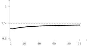
Figure 5.1. The quotient $\gamma(d+1)/\gamma(d)$, for $2\leq d\leq 94\,$. The limit is $2/e\,$.

Remark 5.4.

As shown in Figure 5.1, a classical asymptotics for $j_{\nu,1}$ gives, after observing that

$$\lim_{d\to+\infty}\frac{\gamma(d+1)}{\gamma(d)}=\sqrt{\lim_{d\to+\infty}\frac{\gamma(d+2)}{\gamma(d)}}$$

the following limiting value for the quotient $\gamma(d+1)/\gamma(d)$:

$$\lim_{d\to+\infty}\frac{\gamma(d+1)}{\gamma(d)}=\frac{2}{e}\,.$$

References

- [1] M.S. Ashbaugh and R.D. Benguria. A sharp bound for the ratio of the first two eigenvalues of Dirichlet Laplacians and extensions. Annals of Mathematics, 135(3), (1992), 601–628.
- [2] M. Ashu. Some properties of Bessel functions with applications to Neumann eigenvalues in the unit disc. Bachelor’s thesis 2013:K1 (E. Wahlén advisor), Lund University. http://lup.lub.lu.se/student-papers/record/7370411.
- [3] P. Bérard, D. Meyer. Inégalités isopérimétriques et applications. Ann. Sci. École Norm. Sup. (4) 15(3) (1982) 513–541.
- [4] V. Bonnaillie-Noël, B. Helffer. Nodal and spectral minimal partitions–The state of the art in 2015 (chapter for a book in preparation). A. Henrot (editor). hal-01167181v1.
- [5] L. G. Chambers. An upper bound for the first zero of Bessel functions. Math. Comp., 38(158), (1982), 589–591.
- [6] R. Courant. Ein allgemeiner Satz zur Theorie der Eigenfunktionen selbstadjungierter Differentialausdrücke. Nachr. Ges. Göttingen (1923) 81–84.
- [7] B. Helffer, T. Hoffmann-Ostenhof, and S. Terracini. Nodal domains and spectral minimal partitions. Ann. Inst. H. Poincaré Anal. Non Linéaire 26 (2009) 101–138.
- [8] B. Helffer, T. Hoffmann-Ostenhof, and S. Terracini. Nodal minimal partitions in dimension 3. DCDS-A (Vol. 28, No. 2, 2010) special issues Part I, dedicated to Professor Louis Nirenberg on the occasion of his 85th birthday.
- [9] B. Helffer, T. Hoffmann-Ostenhof, and S. Terracini. On spectral minimal partitions : the case of the sphere. Around the Research of Vladimir Maz’ya III, International Math. Series. 13, 153–179 (2010).
- [10] B. Helffer, R. Kiwan. Dirichlet eigenfunctions on the cube, sharpening the Courant nodal inequality. ArXiv:1506.05733. To appear in the volume “Functional Analysis and Operator Theory for Quantum Physics”, to be published by EMS on the occasion of the 70th birthday of Pavel Exner.
- [11] B. Helffer, M. Persson-Sundqvist. Nodal domains in the square—the Neumann case. arXiv 1410.6702 (2014). To appear in Moscow Mathematical Journal.
- [12] A. Henrot. Extremum problems for eigenvalues of elliptic operators. Frontiers in Mathematics. Birkhäuser Verlag, Basel, 2006.
- [13] J. T. Lewis and M. E. Muldoon. Monotonicity and convexity properties of zeros of Bessel functions. SIAM J. Math. Anal., 8(1), (1977), 171–178.
- [14] J. Leydold. Knotenlinien und Knotengebiete von Eigenfunktionen. Diplomarbeit. 1989.
- [15] J. Leydold. On the number of nodal domains of spherical harmonics. Topology 35, (1996), 301–321.
- [16] J. Peetre. A generalization of Courant’s nodal domain theorem. Math. Scand. 5, (1957), 15–20.
- [17] Å. Pleijel. Remarks on Courant’s nodal theorem. Comm. Pure. Appl. Math., 9, (1956), 543–550.
- [18] M. B. Porter. On the roots of the hypergeometric and Bessel’s functions. Amer. J. Math., 20, (1898), 193–214.
- [19] I. Polterovich. Pleijel’s nodal domain theorem for free membranes. Proc. Amer. Math. Soc. 137(3) (2009) 1021–1024.
- [20] A. B. Shidlovskii. Transcendental numbers. Vol. 12 of de Gruyter Studies in Mathematics, Walter de Gruyter & Co., Berlin, 1989. Translated from the Russian by Neal Koblitz, with a foreword by W. Dale Brownawell.
- [21] M. A. Shubin. Asymptotic behaviour of the spectral function. In Pseudodifferential Operators and Spectral Theory, pages 133–173. Springer Berlin Heidelberg, 2001.
- [22] C. L. Siegel. Über einige Anwendungen diophantischer Approximationen, Abh. Preuss. Akad. Wiss., Phys.-math. Kl., (1929). Reprinted in Gesammelte Abhandlungen I, Berlin-Heidelberg-New York: Springer-Verlag, 1966.
- [23] N. Soave, S. Terracini. Liouville theorems and -dimension symmetry for solutions of an elliptic system modelling phase separation. Adv. Math., 279, (2015), 29-66.
- [24] J. Toth and S. Zelditch. Counting nodal lines which touch the boundary of an analytic domain. J. Differential Geom. 81(3) (2009), 649–686.
- [25] G. Watson. A treatise on the theory of Bessel functions. 2nd ed. London: Cambridge University Press. VII, 1966.