Vacuum stability with spontaneous violation of lepton number

Abstract

The vacuum of the Standard Model is known to be unstable for the measured values of the top and Higgs masses. Here we show how vacuum stability can be achieved naturally if lepton number is violated spontaneously at the TeV scale. More precise Higgs measurements in the next LHC run should provide a crucial test of our symmetry breaking scenario. In addition, these schemes typically lead to enhanced rates for processes involving lepton flavour violation.

I Introduction

The vacuum of the Standard Model (SM) scalar potential is unstable since at high energies the Higgs effective quartic coupling is driven to negative values by the renormalization group flow Alekhin et al. (2012); Buttazzo et al. (2013). Nevertheless, the SM cannot be a complete theory of Nature for various reasons, one of which is that neutrinos need to be massive in order to account for neutrino oscillation results Forero et al. (2014).

With only the SM fields, neutrino masses can arise in a model-independent way from a dimension 5 effective operator $\kappa LLHH$ which gives rise to a $\kappa\left\langle H\right\rangle^{2}$ neutrino mass after electroweak symmetry breaking Weinberg (1979). This same operator unavoidably provides a correction to the Higgs self-coupling $\lambda$ below the scale of the mechanism of neutrino mass generation through the diagram in Fig. 1. Although tiny and negative, it suggests that the mechanism responsible for generating neutrino masses and lepton number violation is potentially relevant for the Higgs stability problem. The quantitative effect of neutrino masses on the stability of the scalar potential will, however, be dependent on the ultra-violet completion of the model.

Figure 1: Contribution of Weinberg’s effective operator to the Higgs quartic interaction.

After the historic Higgs boson discovery at CERN and the confirmation of the Brout-Englert-Higgs mechanism, it is natural to imagine that all symmetries in Nature are broken spontaneously by the vacuum expectation values of scalar fields. The charge neutrality of neutrinos suggests them to be Majorana fermions Schechter and Valle (1980), and that the smallness of their mass is due to the feeble breaking of lepton number symmetry. Hence we need generalized electroweak breaking sectors leading to the double breaking of electroweak and lepton number symmetries.

In this letter we examine the vacuum stability issue within the simplest of such extended scenarios , showing how one can naturally obtain a fully consistent behavior of the scalar potential at all scales for lepton number broken spontaneously at the TeV scale. Note that within the simplest $\mathrm{SU(3)_{c}\otimes SU(2)_{L}\otimes U(1)_{Y}}$ gauge structure lepton number is a global symmetry whose spontaneous breaking implies the existence of a physical Goldstone boson, generically called majoron and denoted $J$, which must be a gauge singlet Chikashige et al. (1981); Schechter and Valle (1982) in order to comply with LEP restrictions Olive et al. (2014). Its existence brings in new invisible Higgs boson decays Joshipura and Valle (1993)

$$H\to JJ,$$

leading to potentially sizable rates for missing momentum signals at accelerators de Campos et al. (1999); Abdallah et al. (2004a, b) including the current LHC Bonilla et al. (2015). Given the agreement of the ATLAS and CMS results with the SM scenario, one can place limits on the presence of such invisible Higgs decay channels. Current LHC data on Higgs boson physics still leaves room to be explored at the next run.

Absolute stability of the scalar potential is attainable as a result of the presence of the Majoron, which is part of a complex scalar singlet. Indeed, it is well known that generically the quartic coupling which controls the mixing between a scalar singlet and the Higgs doublet contributes positively to the value of the Higgs quartic coupling (which we shall call $\lambda_{2}$) at high energies Casas et al. (2000); Elias-Miro et al. (2011, 2012); Basso et al. (2010); Gonderinger et al. (2010); Lebedev (2012); Falkowski et al. (2015); Ballesteros and Tamarit (2015); Delle Rose et al. (2015) — see diagram A in figure 2. On the other hand, new fermions coupling to the Higgs field $H$, such as right-handed neutrinos Elias-Miro et al. (2012); Salvio (2015); Casas et al. (2000), tend to destabilize $\lambda_{2}$ not only through the 1-loop effect depicted in diagram $\textrm{B}_{1}$ of figure 2, but also in what is effectively a two-loop effect (diagram $\textrm{B}_{2}$): through their Yukawa interaction with $H$, the new fermions soften the fall of the top Yukawa coupling at higher energies, which in turn contributes negatively to $\lambda_{2}$ . The model we consider below is a low–scale version of the standard type I majoron seesaw mechanism, such as the inverse seesaw type Mohapatra and Valle (1986); Gonzalez-Garcia and Valle (1989). We stress however that, even though our renormalization group equations (RGEs) are the same as those characterizing standard case, the values of the Dirac–type neutrino Yukawa couplings are typically much higher in our inverse seeaw scenario.

Figure 2: In models with a complex singlet scalar $\sigma$, such as majoron type-I seesaw schemes, the positive contribution to the RGE of the Higgs quartic coupling (diagram A) is accompanied by the destabilizing effect of right-handed neutrinos through the 1-loop diagram $\textrm{B}_{1}$ and also through the two-loop diagram $\textrm{B}_{2}$.

II Electroweak breaking with spontaneous lepton number violation

The simplest scalar sector capable of driving the double breaking of electroweak and lepton number symmetry consists of the SM doublet $H$ plus a complex singlet $\sigma$, leading to the following Higgs potential Joshipura and Valle (1993)

$$V\left(\sigma,H\right)=\mu_{1}^{2}\left|\sigma\right|^{2}+\mu_{2}^{2}H^{\dagger}H+\lambda_{1}\left|\sigma\right|^{4}$$

$$\ \ +\lambda_{2}\left(H^{\dagger}H\right)^{2}+\lambda_{12}\left(H^{\dagger}H\right)\left|\sigma\right|^{2}\,.$$ (1)

In addition to the $\mathrm{SU(3)_{c}\otimes SU(2)_{L}\otimes U(1)_{Y}}$ gauge invariance, $V\left(\sigma,H\right)$ has a global U(1) symmetry which will be associated to lepton number within specific model realizations. The potential is bounded from below provided that $\lambda_{1}$, $\lambda_{2}$ and $\lambda_{12}+2\sqrt{\lambda_{1}\lambda_{2}}$ are positive; these are less constraining conditions than those required for the existence of a consistent electroweak and lepton number breaking vacuum where both $H$ and $\sigma$ adquire non-zero vacuum expectation values ($\equiv\frac{v_{H}}{\sqrt{2}}$ and $\frac{v_{\sigma}}{\sqrt{2}}$). For that to happen, $\lambda_{1}$, $\lambda_{2}$ and $4\lambda_{1}\lambda_{2}-\lambda_{12}^{2}$ need to be all positive . Three of the degrees of freedom in $H$ are absorbed by the massive electroweak gauge bosons, as usual. On the other hand, the imaginary part of $\sigma$ becomes the Nambu-Goldstone boson associated to the breaking of the global lepton number symmetry, therefore it remains massless. As for the real oscillating parts of $H^{0}$ and $\sigma$, these lead to two CP-even mass eigenstates $H_{1}$ and $H_{2}$, with a mixing angle $\alpha$ which can be constrained from LHC data Aad et al. (2014); Chatrchyan et al. (2014); CMS (2015); Bonilla et al. (2015). We take the lighter state $H_{1}$ to be the 125 GeV Higgs particle recently discovered by the CMS and ATLAS collaborations.

Using the renormalization group equations (given in the appendix) we evolved the three quartic couplings of the model imposing the vacuum stability conditions mentioned previously. Given that such equations rely on perturbation theory, the calculations were taken to be trustable only in those cases where the running couplings do not exceed $\sqrt{4\pi}$.

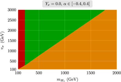
Figure 3: Values of $m_{H_{2}}$ and $v_{\sigma}$ leading to a potential bounded from below (in green on top), a Landau pole at some energy scale (in orange, next), or an unstable potential (in red, last).

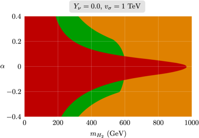
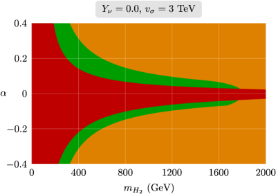
Figure 4: Values of $m_{H_{2}}$ and $\alpha$ leading to a potential bounded from below (in green), a Landau pole at some energy scale (in orange), or an unstable potential (in red). Comparing top and bottom panels shows the effect of changing $v_{\sigma}$.

III Neutrino mass generation

In order to assign to the U(1) symmetry present in Eq. (II) the role of lepton number we must couple the new scalar singlet to leptonic fields. This can be done in a variety of ways. Here we focus on low-scale generation of neutrino mass Boucenna et al. (2014). For definitiveness we choose to generate neutrino masses through the inverse seesaw mechanism Mohapatra:1986bd with spontaneous lepton number violation Gonzalez-Garcia and Valle (1989).

The fermion content of the Standard Model is augmented by right-handed neutrinos $\nu_{R}$ (with lepton number +1) and left-handed gauge singlets $S$ (also with lepton number +1) such that the mass term $\nu_{R}^{c}S$ as well as the interactions $SS\sigma$ and $H\nu_{R}^{c}L$ are allowed if $\sigma$ carries -2 units of lepton number:

$$-\mathscr{L}_{\nu}=Y_{\nu}H\nu_{R}^{c}L+M\nu_{R}^{c}S+Y_{S}SS\sigma+\textrm{h.c.}$$ (2)

The effective neutrino mass, in the one family approximation, is given by the expression

$$m_{\nu}=Y_{S}\left\langle\sigma\right\rangle\left(\frac{Y_{\nu}\left\langle H^{0}\right\rangle}{M}\right)^{2}\,,$$ (3)

which shows that the smallness of the neutrino masses can be attributed to a small (but natural) $Y_{S}$ coupling, while still having $Y_{\nu}$ of order one and both $\left\langle\sigma\right\rangle$, $M$ in the TeV range.

IV Interplay between neutrino mass and Higgs physics

In most cases, the stability of the potential is threatened by the violation of the condition $\lambda_{2}>0$, as in the Standard Model. Instability can be avoided with a large $\lambda_{12}$, which might, however, lead to an unacceptably large mixing angle $\alpha$ between the two CP-even Higgs mass eigenstates Falkowski et al. (2015). In such cases, one must rely instead on a heavy $H_{2}$ — see the green region in Figs. 3–5. Indeed, within the red regions therein, the potential becomes unbounded from below at some high energy scale, just like in the Standard Model. This happens for relatively small values of either $\alpha$ or $m_{H_{2}}$. As a result, a tight experimental bound on $\alpha$ can be used to place a lower limit on the mass of the heavier CP-even scalar. From Fig. 3 one can also see that the lepton breaking scale $v_{\sigma}\equiv\sqrt{2}\left\langle\sigma\right\rangle$ must not be too low, otherwise a big ratio $m_{H_{2}}/\left\langle\sigma\right\rangle$ will lead to the existence of a Landau pole in the running parameters of the model before the Planck scale is reached (shown in orange). This also accounts for the difference between the two plots in Fig. 4.

As far as the neutrino sector is concerned, since $Y_{S}$ is taken to be small, this parameter has no direct impact on the potential’s stability. However, it should be noted that in order to obtain neutrino masses in the correct range, the values of both $v_{\sigma}$ and $Y_{\nu}$ will depend on the one of $Y_{S}$. In principle then, $Y_{\nu}$ might be large, but not too large, as $\left|Y_{\nu}\right|\gtrsim 0.6$ leads to either unstable or non-perturbative dynamics. A non-zero Dirac neutrino Yukawa coupling has a destabilizing effect on the scalar potential which is visible in the recession of the green region to bigger values of $\alpha$ and $m_{H_{2}}$, when comparing the bottom plot in Fig. 4 and the one in Fig. 5.

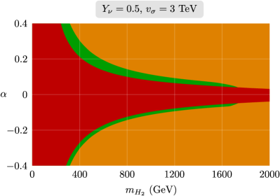
Figure 5: Same as in the bottom plot of Fig. 4, but with $Y_{\nu}\neq 0$.

Another interesting possibility is to have a negligible $Y_{\nu}$ and potentially sizeable $Y_{S}$. In this case, if we keep $M$ of the order of the TeV, we find that the region of stability and perturbativity (shown in green in Fig. 6) depends significantly upon the parameter $Y_{S}$ characterizing spontaneous lepton number violation and neutrino mass generation through $\left\langle\sigma\right\rangle$. To be more precise, as shown in Fig. 6 the allowed values for the mass of the heavy scalar boson ($m_{H_{2}}$) varies with this Yukawa coupling; for example, if $m_{H_{2}}$ was to be found to be, say, $\sim 2$ TeV ($v_{\sigma}=3$ TeV by assumption here), then one would conclude that either $Y_{S}\sim 0.5$ or the scalar sector must be strongly interacting.

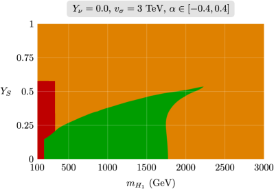
Figure 6: The region stability and perturbativity for the case of non-zero $Y_{S}>0$ and very small $Y_{\nu}$ is displayed in green; the color ordering code is the same as in the scan in Fig. 3.

V Conclusions

In conclusion, the Standard Model vacuum is unstable for the measured top and Higgs boson masses. However the theory is incomplete as it has no masses for neutrinos. We have therefore generalized its symmetry breaking potential in order to induce naturally small neutrino masses from the breaking of lepton number. We have examined the vacuum stability issue in schemes with spontaneous breaking of global lepton number at the TeV scale, showing how one can naturally obtain a consistent behavior of the scalar potential at all scales, avoiding the vacuum instability. Given that the new physics parameters of the theory are not known, it sufficed for us to adopt one-loop renormalization group equations. Since all new particles in the model lie at the TeV scale, they can be probed with current experiments, such as the LHC. Invisible decays of the two CP-even Higgs bosons, $H_{i}\to JJ$, were discussed in Bonilla et al. (2015). Improved sensitivity is expected from the 13 TeV run of the LHC. In addition, we expect enhanced rates for lepton flavour violating processes Bernabeu et al. (1987); Deppisch and Valle (2005); Deppisch et al. (2006). In summary, schemes such as the one explored in this letter may shed light on two important drawbacks of the Standard Model namely, the instability associated to its gauge symmetry breaking mechanism and the lack of neutrino mass.

Acknowledgements

We thank Sofiane Boucenna for discussions in the early phase of this project. This work was supported by MINECO grants FPA2014-58183-P, Multidark CSD2009-00064 and the PROMETEOII/2014/084 grant from Generalitat Valenciana.

VI Appendix A

In this appendix we provide some details on the scalar sector of the model. The potential in equation (II) is controlled by 5 parameters ($\mu_{1}^{2}$, $\mu_{2}^{2}$, $\lambda_{1}$, $\lambda_{2}$, and $\lambda_{12}$) which one can translate into two vacuum expectation values ($v_{\sigma}=\sqrt{2}\left\langle\textrm{Re}\left(\sigma\right)\right\rangle$ and $v_{H}=\sqrt{2}\left\langle\textrm{Re}\left(H^{0}\right)\right\rangle$), two mass eigenvalues ($m_{H_{1}}$ and $m_{H_{2}}$) and a mixing angle $\alpha$:

$$\lambda_{1} =\frac{m_{H_{1}}^{2}\cos^{2}\alpha+m_{H_{2}}^{2}\sin^{2}\alpha}{2v_{\sigma}^{2}}\,,$$ (4)

$$\lambda_{2} =\frac{m_{H_{1}}^{2}\sin^{2}\alpha+m_{H_{2}}^{2}\cos^{2}\alpha}{2v_{H}^{2}}\,,$$ (5)

$$\lambda_{12} =\frac{\left(m_{H_{1}}^{2}-m_{H_{2}}^{2}\right)\cos\alpha\sin\alpha}{v_{\sigma}v_{H}}\,,$$ (6)

$$-\mu_{1}^{2} =\frac{v_{H}\cos\alpha\sin\alpha\left(m_{H_{1}}^{2}-m_{H_{2}}^{2}\right)+m_{H_{1}}^{2}v_{\sigma}\cos^{2}\alpha+m_{H_{2}}^{2}v_{\sigma}\sin^{2}\alpha}{2v_{\sigma}}\,,$$ (7)

$$-\mu_{2}^{2} =\frac{v_{\sigma}\cos\alpha\sin\alpha\left(m_{H_{1}}^{2}-m_{H_{2}}^{2}\right)+m_{H_{1}}^{2}v_{H}\sin^{2}\alpha+m_{H_{2}}^{2}v_{H}\cos^{2}\alpha}{2v_{H}}\,,$$ (8)

with

$$\left(\begin{array}[]{c}H_{1}\\ H_{2}\end{array}\right) \equiv\left(\begin{array}[]{cc}\cos\alpha&\sin\alpha\\ -\sin\alpha&\cos\alpha\end{array}\right)\left(\begin{array}[]{c}\sqrt{2}\textrm{Re}\left(\sigma\right)\\ \sqrt{2}\textrm{Re}\left(H^{0}\right)\end{array}\right)\,.$$ (15)

On the other hand, it is well known that the Standard Model potential is controlled by just two parameters $\mu^{2}$ and $\lambda$:

$$V_{SM}\left(H\right) =\mu^{2}\left(H^{\dagger}H\right)+\lambda\left(H^{\dagger}H\right)^{2}\,.$$ (16)

For a reasonably small mixing angle $\alpha$, one can consider that the state $H_{1}$ is mostly made of the real part of the singlet, hence we may integrate out $\sqrt{2}\textrm{Re}\left(\sigma\right)$. In this approximation, we note that

$$\lambda \approx\lambda_{2}-\frac{\lambda_{12}^{2}}{4\lambda_{1}}\,,$$ (17)

$$\mu^{2} \approx\mu_{2}^{2}-\frac{\lambda_{12}}{2\lambda_{1}}\mu_{1}^{2}\,,$$ (18)

at the scale of decoupling, meaning in particular that there is a tree-level threshold correction between $\lambda_{2}$ and the Standard Model quartic coupling $\lambda$. For the results in this paper, we neglect altogether the small Standard Model range between the $m_{Z}$ and $m_{H_{1}}$ scale, starting instead with equations (4)–(8), which already include this threshold effect.

VII Appendix B

For completeness, we write down here the renormalization group equations of the model parameters which are relevant for the study of the potential’s stability. We work with the 1-family approximation, ignoring the bottom and tau Yukawa couplings. These equations were obtained with the SARAH program Staub (2015) (see also Lyonnet et al. (2014)) and explicitly checked by us using the results in Luo et al. (2003); furthermore they are consistent with Elias-Miro et al. (2012). As usual, $t$ stands for the natural logarithm of the energy scale.

$$\left(4\pi\right)^{2}\frac{dg_{i}}{dt} = b_{i}g_{i}^{3}\text{ with}\ \ b_{i}=\left(\frac{41}{10},-\frac{19}{6},-7\right)\,,$$ (19)

$$\left(4\pi\right)^{2}\frac{dY_{t}}{dt} = \left(-\frac{17}{20}g_{1}^{2}-\frac{9}{4}g_{2}^{2}-8g_{3}^{2}+\frac{9}{2}Y_{t}^{2}+Y_{\nu}^{2}\right)Y_{t}\,,$$ (20)

$$\left(4\pi\right)^{2}\frac{dY_{\nu}}{dt} = \left(-\frac{9}{20}g_{1}^{2}-\frac{9}{4}g_{2}^{2}+3Y_{t}^{2}+\frac{5}{2}Y_{\nu}^{2}\right)Y_{\nu}\,,$$ (21)

$$\left(4\pi\right)^{2}\frac{dY_{S}}{dt} = 6Y_{S}^{3}\,,$$ (22)

$$\left(4\pi\right)^{2}\frac{d\lambda_{1}}{dt} = 20\lambda_{1}^{2}+2\lambda_{12}^{2}+8\lambda_{1}Y_{S}^{2}-16Y_{S}^{4}\,,$$ (23)

$$\left(4\pi\right)^{2}\frac{d\lambda_{2}}{dt} = \frac{27}{200}g_{1}^{4}+\frac{9}{20}g_{1}^{2}g_{2}^{2}+\frac{9}{8}g_{2}^{4}$$

$$- \left(\frac{9}{5}g_{1}^{2}+9g_{2}^{2}\right)\lambda_{2}+24\lambda_{2}^{2}+\lambda_{12}^{2}$$

$$+ \lambda_{2}\left(12Y_{t}^{2}+4Y_{\nu}^{2}\right)-\left(6Y_{t}^{4}+2Y_{\nu}^{4}\right)\,,$$

$$\left(4\pi\right)^{2}\frac{d\lambda_{12}}{dt} = \left[-\left(\frac{9}{10}g_{1}^{2}+\frac{9}{2}g_{2}^{2}\right)+6Y_{t}^{2}+2Y_{\nu}^{2}\right.$$ (25)

$$+ \left.4Y_{S}^{2}+8\lambda_{1}+12\lambda_{2}+4\lambda_{12}\vphantom{\left(\frac{9}{10}g_{1}^{2}+\frac{9}{2}g_{2}^{2}\right)}\right]\lambda_{12}\,.$$

References

- Alekhin et al. (2012) S. Alekhin, A. Djouadi, and S. Moch, Phys.Lett. B716, 214 (2012), arXiv:1207.0980 [hep-ph] .
- Buttazzo et al. (2013) D. Buttazzo, G. Degrassi, P. P. Giardino, G. F. Giudice, F. Sala, et al., JHEP 1312, 089 (2013), arXiv:1307.3536 [hep-ph] .
- Forero et al. (2014) D. Forero, M. Tortola, and J. Valle, Phys.Rev. D90, 093006 (2014), arXiv:1405.7540 [hep-ph] .
- Branchina and Messina (2013) V. Branchina and E. Messina, Phys. Rev. Lett. 111, 241801 (2013), arXiv:1307.5193 [hep-ph] .
- Weinberg (1979) S. Weinberg, Phys.Rev.Lett. 43, 1566 (1979).
- Schechter and Valle (1980) J. Schechter and J. Valle, Phys.Rev. D22, 2227 (1980).
- Costa et al. (2015) R. Costa, A. P. Morais, M. O. P. Sampaio, and R. Santos, Phys. Rev. D92, 025024 (2015), arXiv:1411.4048 [hep-ph] .
- Chikashige et al. (1981) Y. Chikashige, R. N. Mohapatra, and R. D. Peccei, Phys. Lett. B98, 265 (1981).
- Schechter and Valle (1982) J. Schechter and J. Valle, Phys.Rev. D25, 774 (1982).
- Olive et al. (2014) K. Olive et al. (Particle Data Group), Chin.Phys. C38, 090001 (2014).
- Joshipura and Valle (1993) A. S. Joshipura and J. Valle, Nucl.Phys. B397, 105 (1993).
- de Campos et al. (1999) F. de Campos, O. J. P. Eboli, M. A. Garcia-Jareno, and J. W. F. Valle, Nucl. Phys. B546, 33 (1999), hep-ph/9710545 .
- Abdallah et al. (2004a) J. Abdallah et al. (DELPHI Collaboration), Eur.Phys.J. C38, 1 (2004a), arXiv:hep-ex/0410017 [hep-ex] .
- Abdallah et al. (2004b) J. Abdallah et al. (DELPHI collaboration), Eur. Phys. J. C32, 475 (2004b), hep-ex/0401022 .
- Bonilla et al. (2015) C. Bonilla, J. W. F. Valle, and J. C. Romao, (2015), arXiv:1502.01649 [hep-ph] .
- Casas et al. (2000) J. Casas, V. Di Clemente, A. Ibarra, and M. Quiros, Phys.Rev. D62, 053005 (2000), arXiv:hep-ph/9904295 [hep-ph] .
- Elias-Miro et al. (2011) J. Elias-Miro, J. R. Espinosa, G. F. Giudice, G. Isidori, A. Riotto, et al., (2011), arXiv:1112.3022 [hep-ph] .
- Elias-Miro et al. (2012) J. Elias-Miro, J. R. Espinosa, G. F. Giudice, H. M. Lee, and A. Strumia, JHEP 1206, 031 (2012), arXiv:1203.0237 [hep-ph] .
- Basso et al. (2010) L. Basso, S. Moretti, and G. M. Pruna, Phys. Rev. D82, 055018 (2010), arXiv:1004.3039 [hep-ph] .
- Gonderinger et al. (2010) M. Gonderinger, Y. Li, H. Patel, and M. J. Ramsey-Musolf, JHEP 01, 053 (2010), arXiv:0910.3167 [hep-ph] .
- Lebedev (2012) O. Lebedev, Eur.Phys.J. C72, 2058 (2012), arXiv:1203.0156 [hep-ph] .
- Falkowski et al. (2015) A. Falkowski, C. Gross, and O. Lebedev, JHEP 1505, 057 (2015), arXiv:1502.01361 [hep-ph] .
- Ballesteros and Tamarit (2015) G. Ballesteros and C. Tamarit, JHEP 09, 210 (2015), arXiv:1505.07476 [hep-ph] .
- Delle Rose et al. (2015) L. Delle Rose, C. Marzo, and A. Urbano, JHEP 12, 050 (2015), arXiv:1506.03360 [hep-ph] .
- Salvio (2015) A. Salvio, Phys. Lett. B743, 428 (2015), arXiv:1501.03781 [hep-ph] .
- Mohapatra and Valle (1986) R. N. Mohapatra and J. W. F. Valle, Phys. Rev. D34, 1642 (1986).
- Gonzalez-Garcia and Valle (1989) M. C. Gonzalez-Garcia and J. W. F. Valle, Phys. Lett. B216, 360 (1989).
- Aad et al. (2014) G. Aad et al. (ATLAS Collaboration), Phys.Rev.Lett. 112, 201802 (2014), arXiv:1402.3244 [hep-ex] .
- Chatrchyan et al. (2014) S. Chatrchyan et al. (CMS), Eur. Phys. J. C74, 2980 (2014), arXiv:1404.1344 [hep-ex] .
- CMS (2015) Search for invisible decays of Higgs bosons in the vector boson fusion production mode, Tech. Rep. CMS-PAS-HIG-14-038 (CERN, Geneva, 2015).
- Degrassi et al. (2012) G. Degrassi, S. Di Vita, J. Elias-Miro, J. R. Espinosa, G. F. Giudice, G. Isidori, and A. Strumia, JHEP 08, 098 (2012), arXiv:1205.6497 [hep-ph] .
- Boucenna et al. (2014) S. M. Boucenna, S. Morisi, and J. W. Valle, Adv.High Energy Phys. 2014, 831598 (2014), arXiv:1404.3751 [hep-ph] .
- Bernabeu et al. (1987) J. Bernabeu et al., Phys. Lett. B187, 303 (1987).
- Deppisch and Valle (2005) F. Deppisch and J. W. F. Valle, Phys. Rev. D72, 036001 (2005), hep-ph/0406040 .
- Deppisch et al. (2006) F. Deppisch, T. S. Kosmas, and J. W. F. Valle, Nucl. Phys. B752, 80 (2006), hep-ph/0512360 .
- Staub (2015) F. Staub, (2015), arXiv:1503.04200 [hep-ph] .
- Lyonnet et al. (2014) F. Lyonnet, I. Schienbein, F. Staub, and A. Wingerter, Comput. Phys. Commun. 185, 1130 (2014), arXiv:1309.7030 [hep-ph] .
- Luo et al. (2003) M.-x. Luo, H.-w. Wang, and Y. Xiao, Phys.Rev. D67, 065019 (2003), arXiv:hep-ph/0211440 [hep-ph] .