Ehrenfest Breakdown of the Mean-field Dynamics of Bose Gases

Abstract

The mean-field dynamics of a Bose gas is shown to break down at time $\tau_{h}=(c_{1}/\gamma)\ln N$ where $\gamma$ is the Lyapunov exponent of the mean-field theory, $N$ is the number of bosons, and $c_{1}$ is a system-dependent constant. The breakdown time $\tau_{h}$ is essentially the Ehrenfest time that characterizes the breakdown of the correspondence between classical and quantum dynamics. This breakdown can be well described by a quantum fidelity defined for one-particle reduced density matrices. Our results are obtained with the formalism in particle-number phase space and are illustrated with a triple-well model. The logarithmic quantum-classical correspondence time may be verified experimentally with Bose-Einstein condensates.

I Introduction

The nonlinear Gross-Pitaevskii equation (GPE), as a mean-field theory, has been the dominant tool in describing the dynamics of Bose-Einstein condensates (BECs) in ultracold atomic gases Dalfovo et al. (1999); Yukalov (2004). However, we face a quandary when the mean-field dynamics of a BEC becomes dynamically unstable or chaotic Wu and Niu (2001); Smerzi et al. (2002); Liu et al. (2006); Manfredi and Hervieux (2008); Reslen et al. (2008); Thommen et al. (2003); Buonsante et al. (2003): on one hand, one may regard this instability as an unphysical artifact resulted from the mean-field approximation, since the exact dynamics of a BEC is governed by the many-body Schrödinger equation, which is linear and thus does not allow chaos; on the other hand, the dynamical instability was observed in experiments Burger et al. (2001); Wu and Niu (2002); Fallani et al. (2004); Gemelke et al. (2005); Zhang et al. (2005a); Bloch (2005) and it has been proved with mathematical rigor that the GPE describes correctly not only the ground state but also the dynamics of a BEC in the large $N$ limit ($N$ is the number of bosons) Lieb et al. (2000); Erdős et al. (2007).

Our aim in this work is to resolve this fundamental dilemma. Our study shows that the mean-field theory (the GPE) is only valid up to time

$$\tau_{h}=\frac{c_{1}}{\gamma}\ln N+o(\ln N),$$ (1)

where $\gamma$ is the Lyapunov exponent of the mean-field dynamics and $c_{1}$ is a constant that depends only on systems. With this time scale, the dilemma is resolved: on one hand, in the large $N$ limit ($N\rightarrow\infty$), $\tau_{h}$ goes to infinity and thus the GPE is always valid just as proved rigorously in Ref. Erdős et al. (2007); on the other hand, the time $\tau_{h}$ increases with $N$ only logarithmically and it is not a long time for a typical BEC experiment. For example, for the system studied in Ref. Wu and Niu (2001), the Lyapunov time $\tau_{\gamma}=1/\gamma\sim 1$ ms. As the number of atoms in a BEC prepared in a typical experiment is around $10^{4}$, we have $\tau_{h}\sim 10$ ms. As a result, the dynamical instability or the breakdown of the mean-field dynamics can be easily observed in a typical experiment as reported in Ref. Fallani et al. (2004).

This time scale $\tau_{h}$ is essentially the Ehrenfest time, which is the time that the correspondence between the classical and quantum dynamics breaks down Berman and Zaslavsky (1978); Silvestrov and Beenakker (2002). The usual Ehrenfest time $\tau_{\mathrm{Eh}}=(c_{1}/\gamma)\ln(A/\hbar)$, where $\gamma$ is the Lyapunov exponent of the classical motion and $A$ is a typical action Silvestrov and Beenakker (2002). The similarity is due to that the GPE can be regarded as a classical equation in the large $N$ limit Yaffe (1982). Therefore, our result paves a way to experimental investigation of a fundamental relation in the quantum-classical correspondence — the logarithmic behavior of the Ehrenfest time — as $N$ can be varied in experiments.

We cast the quantum dynamics onto the particle-number phase space (PNPS), which is a rearrangement of Fock states. In this phase space, for a nearly coherent state and in the large $N$ limit, quantum many-body dynamics is equivalent to an ensemble of mean-field dynamics. When the mean-field motion is regular, mean-field trajectories will stay together and the Bose gas remains coherent. If the mean-field motion is unstable or chaotic, mean-field trajectories will separate soon from each other exponentially, leading to decoherence of Bose gas and breakdown of the mean-field theory. So, there are two distinct types of quantum dynamics, whose difference can be characterized by the quantum fidelity for one-particle reduced density matrices.

We investigate the Ehrenfest breakdown numerically in the system of a BEC in a triple-well potential Nemoto et al. (2000); Franzosi and Penna (2001, 2003); Liu et al. (2007); Guo et al. (2014), which may be the simplest BEC model that embraces chaotic mean-field dynamics. With this model, we verify numerically the Ehrenfest time and show that our quantum fidelity can well capture the characteristics of two different types of quantum dynamics.

The mean-field instability or breakdown has been discussed in literature Liu et al. (2006); Manfredi and Hervieux (2008); Reslen et al. (2008); Wu and Niu (2001); Luo et al. (2007); Habib et al. (1998); Anglin2001 ; Gertjerenken et al. (2010); Weiss and Teichmann (2008); Březinová et al. (2012). However, a general and explicit relation between mean-field chaos, number of particles and breakdown time is still lacking. And in PNPS not only such breakdown can be understood intuitively and quantitatively, but the significance of a local phase structure is also apparent, distortion of which leads to decoherence.

II Particle-number phase space

In Ref. Yaffe (1982), it is shown that many quantum systems become classical in the large $N$ limit. A dilute Bose gas belongs to this class of quantum systems: its dynamics becomes classical and it is well described by the mean-field GPE in the large $N$ limit. In this section, we introduce PNPS, where this quantum-classical correspondence in the large $N$ limit becomes transparent.

II.1 Definition

Any quantum state $\ket{\Psi}$ of a system of $N$ identical bosons with $M$ single-particle states can be regarded as a wavefunction $\varphi(\bm{x})$ over an $(M-1)$-dimensional lattice space, which we call particle number phase space (PNPS), via

$$\varphi(\bm{x})\equiv\bra{0}\prod_{i=1}^{M}\frac{\hat{a}_{i}^{Nx_{i}}}{\sqrt{(Nx_{i})!}}\ket{\Psi}\,,$$ (2)

where $x_{i}$’s are entries of the $M$-dimensional vector $\bm{x}$, $Nx_{i}\in\{0,\ldots,N\}$ for $1\leq i\leq M$ and $\sum_{i}x_{i}=1$. And $\hat{a}_{i}^{\dagger}$ and $\hat{a}_{i}$ are the creation and annihilation operators for the $i$-th single-particle state, with $[\hat{a}_{i},\hat{a}^{\dagger}_{j}]=\delta_{ij}$ and $\hat{n}_{i}\equiv\hat{a}_{i}^{\dagger}\hat{a}_{i}$. The continuous limit of PNPS is a hyperplane in $[0,1]^{M}$ (defined by constraint $\sum_{i=1}^{M}x_{i}=1$), where we can define (for $i$ from $1$ to $M$)

$$\langle x_{i}\rangle\equiv\int\mathrm{d}\bm{x}\,x_{i}|\varphi(\bm{x})|^{2}$$ (3)

$$\langle(\Delta x_{i})^{2}\rangle\equiv\int\mathrm{d}\bm{x}\,(x_{i}-\langle x_{i}\rangle)^{2}|\varphi(\bm{x})|^{2}$$ (4)

to characterize the average position and spread of the distribution $|\varphi(\bm{x})|^{2}$ over PNPS, given $\ket{\Psi}$ normalized. Of course for any finite $N$, the integral should be interpreted as summations over all $\bm{x}$ in PNPS.

As an example of our particular interest, we examine an SU($M$) coherent state $|\Psi\rangle_{c}$ in PNPS:

$$\ket{\Psi}_{c}\equiv\frac{1}{\sqrt{N!}}\left(\sum_{i=1}^{M}\psi_{i}a_{i}^{\dagger}\right)^{N}\ket{0}\,,$$ (5)

where $\sum_{i}|\psi_{i}|^{2}=1$. In such case, we say $\ket{\psi}$ (an $M$-dimensional vector with $\psi_{i}$ as its entries) is the mean-field state of the SU($M$) coherent state $\ket{\Psi}_{c}$. It is straightforward to show for this coherent state $\ket{\Psi}_{c}$

$$\langle x_{i}\rangle=|\psi_{i}|^{2}\,,\quad\langle(\Delta x_{i})^{2}\rangle=|\psi_{i}|^{2}(1-|\psi_{i}|^{2})/N\,,$$ (6)

which indicate that the coherent state $\ket{\Psi}_{c}$ corresponds to a localized distribution $|\varphi(\bm{x})|^{2}$ in PNPS that peaks around $(|\psi_{1}|^{2},|\psi_{2}|^{2},\cdots,|\psi_{M}|^{2})$ with a vanishing spread at large $N$.

And the wavefunction $\varphi(\bm{x})$ in PNPS has a phase structure. For any $\bm{x}$ and $\bm{y}$ in PNPS,

$$\,\mathrm{arg}\,\varphi(\bm{x})-\,\mathrm{arg}\,\varphi(\bm{y})=N\sum_{i=1}^{M}(x_{i}-y_{i})\,\mathrm{arg}\,\psi_{i}\,\,(\textrm{mod }2\pi)\,,$$ (7)

which shows a wavevector $\bm{k}$: $k_{i}=N\,\mathrm{arg}\,\psi_{i}\propto N$. This phase structure is important as it will give us an estimate of the time $\tau_{h}$ in our later discussion. It is worth noting that when $N\to\infty$, there is no limit of the wavefunction $\varphi(\bm{x})$ because its wavevector $\bm{k}$ diverges.

Overall, we find that the coherent state corresponds to a single-peaked wavepacket with plane-wave phase structure in PNPS. In the following, we shall discuss quantum dynamics in PNPS and its relation to the mean-field dynamics. Note that the formalism of PNPS was also used in other contexts Buonsante et al. (2011, 2012), where phase structure and dynamics, however, were not discussed.

II.2 Dynamics

Consider a quite general Hamiltonian of a Bose gas

$$\hat{\mathcal{H}}=\sum_{i,j=1}^{M}\Big{\{}H^{0}_{ij}\hat{a}_{i}^{\dagger}\hat{a}_{j}+\frac{U_{ij}}{N}\hat{a}_{i}^{\dagger}\hat{a}_{j}^{\dagger}\hat{a}_{j}\hat{a}_{i}\Big{\}}\,,$$ (8)

where $H_{ij}^{0}=H_{ji}^{0*}$ and $U_{ij}=U_{ji}$. Corresponding to the Schrödinger equation $i\partial_{t}\ket{\Psi}=\hat{\mathcal{H}}\ket{\Psi}$, there is an equation of motion (EOM) for $\varphi(\bm{x};t)$ in PNPS (Eq. (20) in the Appendix). We are especially interested in the dynamics of a nearly coherent state $\varphi(\bm{x};t)$, which satisfies the following two conditions:

(i) the distribution $|\varphi(\bm{x};t)|^{2}$ is localized such that $1/N\ll\sqrt{\langle(\Delta x_{i})^{2}\rangle}\ll 1$ for all $i=1,2,\ldots,M$;

(ii) a local wavevector $\bm{k}(\bm{x};t)\equiv\nabla_{\bm{x}}\,\mathrm{arg}\,\varphi(\bm{x};t)$ exists in PNPS and varies insignificantly over a scale of $1/N$, i.e., $|\partial_{x_{i}}k_{j}|\ll N$ for all $i,j=1,2,\ldots,M$.

With these two conditions and keeping only finite terms in the large $N$ limit, an approximate (to $\mathcal{O}(1)$) EOM for $\varphi(\bm{x};t)$ in PNPS can be derived (see Eq. (21) in the Appendix). Mathematically, there are $\delta$-function solutions to this EOM (Eq. (21)):

$$\varphi(\bm{x};t)=\exp[i\alpha(t)]\prod_{i=1}^{M}\delta(x_{i}-x^{0}_{i}(t))\exp[ik^{0}_{i}(t)x_{i}]\,.$$ (9)

In these $\delta$-function solutions, $x^{0}_{i}(t)$, $k^{0}_{i}(t)$ satisfy the following equation

$$i\partial_{t}\hat{\rho}=[\hat{\mathcal{H}}_{\mathrm{MF}},\hat{\rho}]\,,$$ (10)

where $\mathcal{H}_{\mathrm{MF},ij}(t)\equiv H^{0}_{ij}+2U_{ij}\rho_{ij}(t)$ and

$$\rho_{ij}(t)\equiv\sqrt{x^{0}_{i}(t)x^{0}_{j}(t)}\,\mathrm{e}^{i(k^{0}_{i}(t)-k^{0}_{j}(t))/N}\,.$$ (11)

This is just the mean-field EOM for the one-particle reduced density matrix.

Conditions (i) and (ii) reflect our expectations of nearly coherent states (see Eqs. (6) and (7)). The existence of $\delta$-function solutions corresponds to the established result that for any time $t_{0}$, when $N\to\infty$, coherent states at $t=0$ stay coherent when $t=t_{0}$ Erdős et al. (2007).

The results above can be interpreted as follows: at large $N$, for any initial state satisfying the two conditions, its time evolution may be regarded as the superposition of mean-field dynamics of $\delta$-functions, since any function in PNPS can be decomposed into a superposition of a cloud of $\delta$-functions! This is similar to the quantum dynamics of a single-particle wavepacket in real space: it can be regarded as a cloud of classical particles and each of them follows the Newton’s EOM.

As the quantum-classical correspondence between a quantum wavepacket and a classical particle will break down at the Ehrenfest time, the correspondence between one state in PNPS and its mean-field description — one $\delta$-function solution (see Eq. (9)) — will also fail when the mean-field trajectories of the $\delta$-functions in the cloud diverge.

The breakdown time $\tau_{h}$ can be estimated using a conventional strategy in quantum chaos as in Ref. Silvestrov and Beenakker (2002). Essentially, before the breakdown the wavepacket of nearly coherent states in PNPS expands in the form of $\exp\gamma t$, where $\gamma$ is the Lyapunov exponent of the mean-field dynamics. According to Eq. (6), for $t<\tau_{h}$,

$$\Delta(t)\equiv\sqrt{\frac{1}{M}\sum_{i=1}^{M}\langle(\Delta x_{i})^{2}\rangle(t)}\propto\frac{\mathrm{e}^{\gamma t}}{\sqrt{N}}\,.$$ (12)

And there is a consistent mean-field description only if local wavevectors across the wavepacket are almost equal, that is,

$$\kappa tN^{-\lambda}\Delta(t)\ll 1\,,$$ (13)

where $\kappa N^{-\lambda}$ is the average rate of growth of curvature $\partial_{x_{i}}k_{j}$ and the $N$ dependence is written explicitly. Substituting (12) into (13), we have

$$\gamma t+\ln t+\ln\kappa\ll\big{(}\lambda+\frac{1}{2}\big{)}\ln N\,.$$ (14)

The Ehrenfest time $\tau_{h}$ in Eq. (1) is obtained with $c_{1}=\lambda+\frac{1}{2}$, which is independent of $N$ or $\gamma$. Numerical verification of this relation will be presented later.

Note that it is well-known that the quantum-classical correspondence may last far beyond the Ehrenfest time (see, e.g., Ref. Karkuszewski et al. (2002)). Similarly, it is possible that the mean-field theory remains valid even after our first estimate $t=\tau_{h}$; this interesting and special topic will be left for future study.

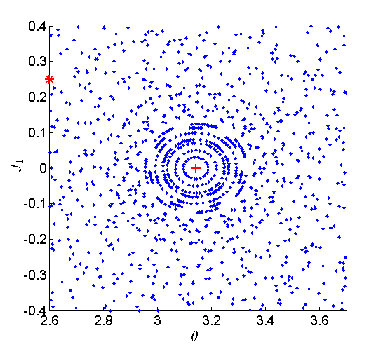
Figure 1: (color online) Poincaré section of the classical (mean-field) triple-well Hamiltonian with conjugate variables $(J_{1},\theta_{1})$ and $(J_{2},\theta_{2})$ at $\theta_{2}=0$, $\dot{\theta}_{2}<0$, $c=1.25$, $E\approx 0.708$. ‘+’ represents a state in the central regular region and ‘*’ represents a state in the chaotic sea.

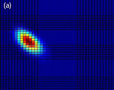
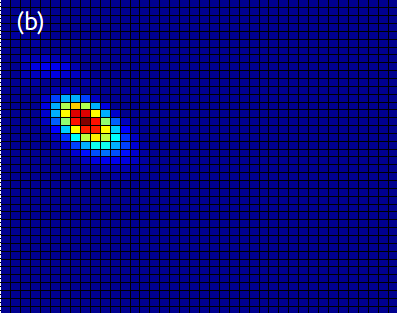
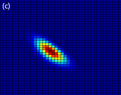
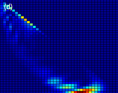
Figure 2: (color online) Plot of $|\varphi(x_{1},x_{2},x_{3};t)|^{2}$ for the quantum triple-well model with $N=40$. Two axes are $x_{1}\in[0,1]$ and $x_{2}\in[0,1]$ ($x_{3}=1-x_{1}-x_{2}$). Red regions are of larger $|\varphi|^{2}$. (a) Initial state corresponding to the mean-field state denoted by ‘+’ in Fig. 1; (b) the ‘+’ state after evolving dynamically $t=14.5$; (c) initial state corresponding to the ‘*’ state in Fig. 1; (d) the ‘*’ state at $t=14.5$.

III Example of Triple-well Model

We now illustrate our results with an example. Consider a BEC in a ring-shaped triple-well potential Guo et al. (2014). Under tight-binding approximation, the second-quantized Hamiltonian is (as a specific case of Eq. (8))

$$\hat{\mathcal{H}}=-\frac{1}{2}\sum_{1\leq i,j\leq 3}^{i\neq j}\hat{a}_{i}^{\dagger}\hat{a}_{j}+\frac{c}{2N}\sum_{i=1}^{3}\hat{a}_{i}^{\dagger}\hat{a}_{i}^{\dagger}\hat{a}_{i}\hat{a}_{i}\,,$$ (15)

where $c$ is the on-site interaction strength. For this system $M=3$. Its corresponding nonlinear mean-field EOM is

$$i\frac{\mathrm{d}}{\mathrm{d}t}\left(\begin{array}[]{c}\psi_{1}\\ \psi_{2}\\ \psi_{3}\\ \end{array}\right)=\left(\begin{array}[]{ccc}c|\psi_{1}|^{2}&-1/2&-1/2\\ -1/2&c|\psi_{2}|^{2}&-1/2\\ -1/2&-1/2&c|\psi_{3}|^{2}\end{array}\right)\left(\begin{array}[]{c}\psi_{1}\\ \psi_{2}\\ \psi_{3}\\ \end{array}\right)\,.$$ (16)

Shown in Fig. 1 is a Poincaré section of the above mean-field dynamics, where two kinds of motion are evident: the central regular region is surrounded by a chaotic sea. The conjugate variables used in plotting Fig. 1 are $(J_{1},\theta_{1})$, $(J_{2},\theta_{2})$, which are defined as $J_{1}=|\psi_{1}|^{2}-|\psi_{3}|^{2}$, $J_{2}=|\psi_{3}|^{2}$, $\theta_{1}=\,\mathrm{arg}\,\psi_{2}-\,\mathrm{arg}\,\psi_{1}$, $\theta_{2}=2\,\mathrm{arg}\,\psi_{2}-\,\mathrm{arg}\,\psi_{1}-\,\mathrm{arg}\,\psi_{3}$.

The quantum dynamics of this model can also be computed rather easily. The evolution of $|\varphi(\bm{x})|^{2}$ in PNPS is plotted in Fig. 2, where two types of quantum dynamics are clearly observed. In Fig. 2 (a, b), an initial coherent state, which is a gaussian-like wavepacket in PNPS, shows no significant expansion or distortion during dynamical evolution. In Fig. 2 (c, d), the situation is drastically different: a similar-looking initial coherent state expands and becomes dramatically distorted after a certain time. The difference is caused by the fact that the initial state in Fig. 2 (a) corresponds to a mean-field state in the regular region in Fig. 1 while the one in Fig. 2 (c) corresponds to a mean-field state in the chaotic region.

It is obvious that the mean-field theory cannot describe the dramatic quantum dynamics shown in Fig. 2 (c, d). Such a failure or breakdown of the mean-field theory due to rapid decoherence has long been noticed in literature Anglin2001 ; Gertjerenken et al. (2010); Weiss and Teichmann (2008); Březinová et al. (2012). In Ref. Weiss and Teichmann (2008), a remedy was tried unsuccessfully to bridge the gap between the mean-field theory and the exact quantum theory. In this work we have shown that there exists a general time scale $\tau_{h}$ in terms of Lyapunov exponent and number of bosons beyond which the mean-field theory fails. In the following, we shall introduce a quantum fidelity to distinguish the two types of quantum dynamics shown in Fig. 2 without using mean-field formalism, and confirm the time scale $\tau_{h}$ numerically.

III.1 Quantum Fidelity

To quantify the loss of coherence in the quantum evolution as shown in Fig. 2 (d), we introduce the following quantum fidelity ${\mathcal{F}}_{q}$ for one-particle reduced density matrix (RDM) $\hat{\rho}$ and $\hat{\chi}$:

$${\mathcal{F}}_{q}(\hat{\rho},\hat{\chi})\equiv\frac{1}{N^{2}}\mathrm{tr}\,\hat{\rho}^{\dagger}\hat{\chi}\,.$$ (17)

For a quantum state $\ket{\Psi(t)}$, its one-particle RDM can be explicitly written as

$$\sum_{ij}\ket{i}\langle\Psi(t)|\hat{a}_{i}^{\dagger}\hat{a}_{j}|\Psi(t)\rangle\bra{j}\,.$$ (18)

There are three reasons to use this quantum fidelity:

1) Experimentally we are often interested in the one-particle RDM.

2) It allows us to define coherence $\mathcal{C}$:

$$\mathcal{C}(\hat{\rho})\equiv{\mathcal{F}}_{q}(\hat{\rho},\hat{\rho})\,,$$ (19)

where $\hat{\rho}$ is the one-particle RDM for $\ket{\Psi}$. The coherence $\mathcal{C}$ can quantify how coherent the state $\ket{\Psi}$ is: $\mathcal{C}(\hat{\rho})=1$ if and only if $\ket{\Psi}$ is a coherent state as in Eq. (5).

3) It returns to the mean-field fidelity for coherent states, i.e., ${\mathcal{F}}_{q}(\hat{\rho},\hat{\chi})={\mathcal{F}}_{\mathrm{mf}}(\psi,\phi)\equiv|\langle\phi|\psi\rangle|^{2}$ if $\hat{\rho}$, $\hat{\chi}$ are one-particle RDM for coherent states $\ket{\Psi}_{c}$ and $\ket{\Phi}_{c}$, and $\psi$, $\phi$ are mean-field states of $\ket{\Psi}_{c}$ and $\ket{\Phi}_{c}$ (see discussion under Eq. (5)). Therefore, before the Ehrenfest breakdown ${\mathcal{F}}_{q}$ essentially captures mean-field characteristics, especially the Lyapunov exponent, which distinguishes regular and chaotic mean-field trajectories.

III.2 Numerical Results

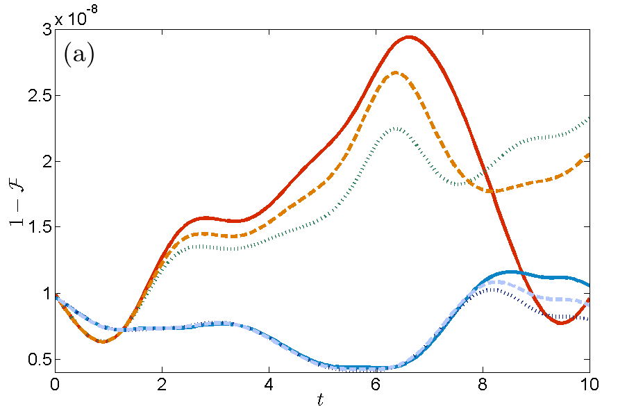
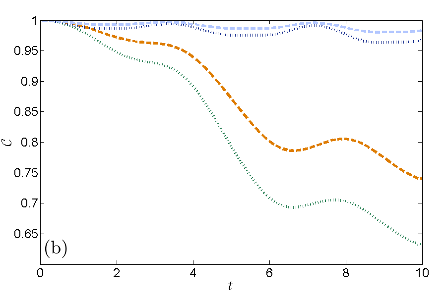
Figure 3: (color online) (a) Quantum and mean-field fidelities. Solid lines are $1-\mathcal{F}_{\mathrm{mf}}(\psi(t),\tilde{\psi}(t))$; dashed lines are $1-\mathcal{F}_{q}(\hat{\rho}(t),\hat{\tilde{\rho}}(t))/\sqrt{\mathcal{F}_{q}(\hat{\rho}(t),\hat{\rho}(t))\mathcal{F}_{q}(\hat{\tilde{\rho}}(t),\hat{\tilde{\rho}}(t))}$ for $N=80$; dotted lines are $1-\mathcal{F}_{q}(\hat{\rho}(t),\hat{\tilde{\rho}}(t))/\sqrt{\mathcal{F}_{q}(\hat{\rho}(t),\hat{\rho}(t))\mathcal{F}_{q}(\hat{\tilde{\rho}}(t),\hat{\tilde{\rho}}(t))}$ for $N=40$. $\mathcal{F}_{q}$ is normalized to better show the correspondence. (b) Coherence $\mathcal{C}(\hat{\rho}(t))$. Curves show the decay of coherence of quantum many-body states in (a). In the simulation, $c=1.25$, $E\approx 0.708$, $\theta_{1}=\pi$, $\theta_{2}=0$, $\hat{\rho}(t)$ and $\hat{\tilde{\rho}}(t)$ are the RDM of quantum states, whose corresponding mean-field states are $|\psi(t)\rangle$ and $|\tilde{\psi}(t)\rangle$, respectively. $\|\psi-\tilde{\psi}\|_{t=0}\approx 10^{-4}$. The lower set of lines in (a) and the corresponding upper set of lines in (b) are for the integrable case $J_{1}=0$; the upper set in (a) and the corresponding lower set in (b) are for the chaotic case $J_{1}=0.5$.

The numerical simulation aims at verifying our theoretical understanding as discussed: for a coherent initial state, at the beginning the mean-field dynamics agrees with the quantum evolution, producing even the same growth of discrepancy between states; however, long-time exponential growth is not allowed by quantum mechanics, so there exists an Ehrenfest time $\tau_{h}$ beyond which the mean-field and quantum correspondence fails. Such a failure is due to the decoherence of quantum states; the breakdown time $\tau_{h}$ is given in Eq. (1). In the following we provide numerical evidences for our theortical understanding.

We choose a coherent initial state $\ket{\Psi(t=0)}_{c}$ with one-particle RDM $\hat{\rho}(t=0)$, whose corresponding mean-field state is $\ket{\psi(t=0)}$. Then we slightly perturb the mean-field state into $\ket{\tilde{\psi}(t=0)}$, and generate the corresponding coherent state $\ket{\tilde{\Psi}(t=0)}_{c}$ and RDM $\hat{\tilde{\rho}}(t=0)$. Next we observe the evolution of quantum fidelity between these two states, which allows us to calculate the Lyapunov exponent. Of course, $\ket{\psi(t)}$ and $\ket{\tilde{\psi}(t)}$ evolve according to the mean-field equations Eq. (16), $\ket{\Psi(t)}$ and $\ket{\tilde{\Psi}(t)}$ evolve according to the quantum Hamiltonian in Eq. (8), $\hat{\rho}(t)$ and $\hat{\tilde{\rho}}(t)$ are obtained from $\ket{\Psi(t)}$ and $\ket{\tilde{\Psi}(t)}$, respectively. $1-{\mathcal{F}}_{q}(\hat{\rho}(t),\hat{\tilde{\rho}}(t))$ and $1-{\mathcal{F}}_{\mathrm{mf}}(\psi(t),\tilde{\psi}(t))$ are shown in Fig. 3 (a), where we see that the mean-field fidelity ${\mathcal{F}}_{\rm mf}$ coincides with ${\mathcal{F}}_{q}$ for small $t$, as expected.

However, we also observe in Fig. 3 (a) that there is an Ehrenfest time $\tau_{h}$, when ${\mathcal{F}}_{q}$ and ${\mathcal{F}}_{\mathrm{mf}}$ start to visibly disagree. Cases for different $N$ and $\gamma$ are plotted in Fig. 3 (a), where we can see that as $N$ increases or $\gamma$ decreases, $\tau_{h}$ gets longer. This qualitatively agrees with the scaling of the Ehrenfest time. And in Fig. 3 (b), it is observed that although $\tau_{h}$ is different for different $N$ and $\gamma$, $\tau_{h}$ is approximately the time when the coherence ${\mathcal{C}}(\hat{\rho}(t))$ drops below 98%. This confirms our understanding that the failure of correspondence between the mean-field and quantum descriptions is the result of decoherence of quantum states.

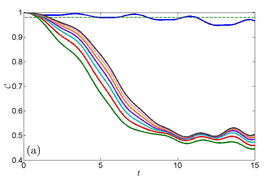
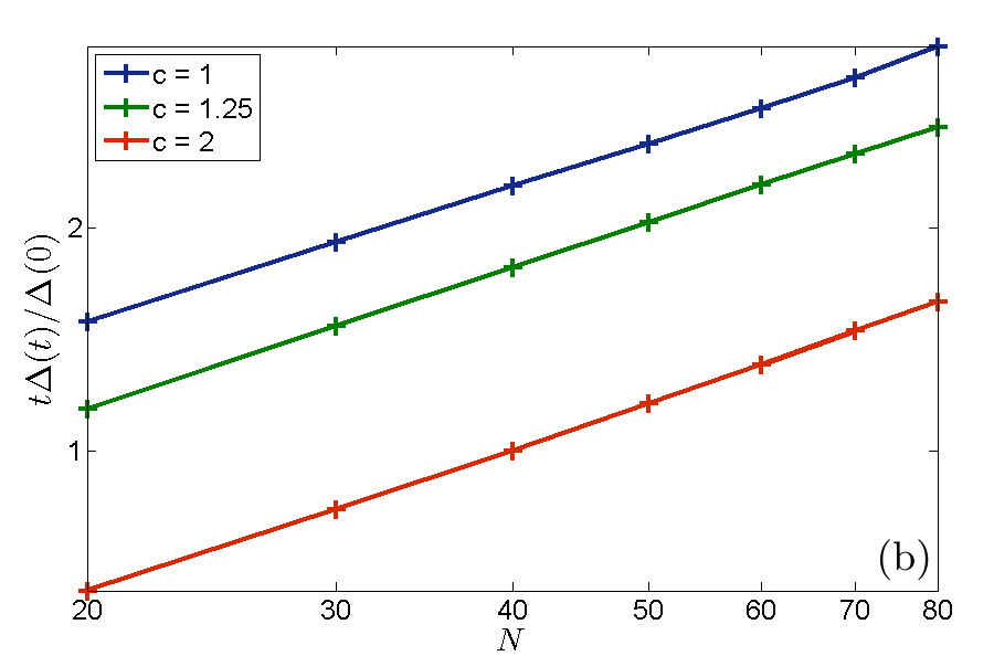
Figure 4: (color online) (a) Time evolution of coherence $\mathcal{C}(\hat{\rho}(t))$ for the integrable $J_{1}=0$ and the chaotic $J_{1}=0.6$ trajectories. $c=1.25$, $E\approx 0.708$, $\theta_{1}=\pi$, $\theta_{2}=0$ and time step in simulation is $10^{-3}$. $\mathcal{C}$ of integrable $J_{1}=0$ (the solid line in the top) remains high while $\mathcal{C}$ of chaotic $J_{1}=0.6$ (other solid lines) drops quickly ($N=20,30,\ldots,80$ from left to right). The dashed line is $\mathcal{C}=98\%$. (b) Linear fitting of $\ln\Delta(t)/\Delta(0)+\ln t+\ln\kappa=c_{1}\ln N$ for the chaotic initial state in (a) with $c=1$, 1.25 and 2, $N$ from 20 to 80. Data points are calculated when $\mathcal{C}$ drops to $98\%$. The slope $c_{1}\approx 0.6$ is found independent of $c$ or $\gamma$.

Based on such understanding, we can quantitatively define the Ehrenfest time in this example as the time when the coherence ${\mathcal{C}}(\hat{\rho}(t))$ drops below 98%. Examples of decay of ${\mathcal{C}}(\hat{\rho}(t))$ is illustrated in Fig. 4 (a), where the Ehrenfest time $\tau_{h}$ is measured when ${\mathcal{C}}(\hat{\rho}(t))$ drops below the dashed line. By varying $N$ and $c$, we verify the relation Eq. (14), which leads to Eq. (1), in Fig. 4 (b). A linear fitting between $\ln\Delta(t)/\Delta(0)+\ln t$ and $\ln N$ is found with a constant slope $\lambda+\frac{1}{2}\approx 0.6$ (see Eq. (14)), suggesting $c_{1}\approx 0.6$ in Eq. (1). Note here $\gamma t$ is replaced by $\ln\Delta(t)/\Delta(0)$ for numerical convenience.

IV Conclusion

In sum we have answered an intriguing question — when does mean-field approximation of a dilute Bose gas remain valid as the system evolves? Our answer is the mean-field dynamics breaks down at the Ehrenfest time $\tau_{h}=(c_{1}/\gamma)\ln N$. The study is facilitated by introducing particle number phase space, where one can see easily that the correspondence between many-body quantum dynamics and mean-field dynamics is similar to the usual quantum-classical correspondence.

As $N$ can be varied in BEC experiments, it is now possible to experimentally measure the logarithmic behavior of the Ehrenfest time. One can compare physical observables in the experiment with their theoretical mean-field values, and measure the Ehrenfest time when their discrepancy exceeds a threshold. BECs with unstable or chaotic mean-field descriptions are suitable for such experiments; for example, spinor BECs Chang et al. (2005); Zhang et al. (2005b) may be a good candidate system.

This work is supported by the National Basic Research Program of China (2013CB921903, 2012CB921300) and the National Natural Science Foundation of China (11274024, 11334001, 11429402).

Appendix A Quantum EOM in PNPS and Its Mean-field Approximation

For the Hamiltonian in Eq. (8), the Schrödinger equation in PNPS reads ($\hbar=1$)

$$i\partial_{t}\varphi(\bm{x};t) = \sum_{i}H^{0}_{ii}Nx_{i}\varphi(\bm{x};t)$$ (20)

$$+ \sum_{i}U_{ii}Nx_{i}(x_{i}-\epsilon)\varphi(\bm{x};t)$$

$$+ \sum_{i\neq j}H^{0}_{ij}N\sqrt{x_{i}(x_{j}+\epsilon)}\varphi(\bm{x}+\epsilon\bm{e}^{ij};t)$$

$$+ \sum_{i\neq j}U_{ij}Nx_{i}x_{j}\varphi(\bm{x};t)\,,$$

where $\epsilon\equiv 1/N$, $\bm{e}^{ij}$ is an $M$-dimensional vector $e^{ij}_{k}\equiv-\delta_{ik}+\delta_{jk}$, $k=1,2,\ldots,M$.

We are especially interested in the dynamics of a nearly coherent state. With conditions (i) and (ii) in Sect. II B and $N\to\infty$, Eq. (20) becomes

$$i\partial_{t}\varphi = \sum_{i}H^{0}_{ii}Nx_{i}\varphi+\sum_{i}U_{ii}Nx_{i}(x_{i}-\epsilon)\varphi$$ (21)

$$+ \sum_{i\neq j}H^{0}_{ij}N\sqrt{x_{i}x_{j}}\varphi\exp[i(k_{j}-k_{i})\epsilon]$$

$$+ \sum_{i\neq j}H^{0}_{ij}\frac{1}{2}\sqrt{\frac{x_{i}}{x_{j}}}\varphi\exp[i(k_{j}-k_{i})\epsilon]$$

$$+ \sum_{i\neq j}H^{0}_{ij}\sqrt{x_{i}x_{j}}[(\partial_{j}-\partial_{i})|\varphi|]\frac{\varphi}{|\varphi|}\exp[i(k_{j}-k_{i})\epsilon]$$

$$+ \sum_{i\neq j}U_{ij}Nx_{i}x_{j}\varphi\,+o(1),$$

where $\partial_{i}\equiv\frac{\partial}{\partial{x_{i}}}$ and $k_{i}(\bm{x};t)$ is the local wavevector of wavefunction $\varphi$ at $(\bm{x};t)$, as discussed in condition (ii). The argument of all $k_{i}$ and $\varphi$ is $(\bm{x};t)$ and omitted.

Now we assume a $\delta$-function solution as in Eq. (9). By equalling the coefficients before $\delta$, $\partial_{i}\delta$ and the derivatives of coefficients before $\delta$ (which is necessary to reflect the plane-wave phase structure) on both sides, keeping finite terms in the large $N$ limit, we obtain

$$\partial_{t}x^{0}_{i} = 2\,\mathrm{Im}\sum_{j}H^{0}_{ij}\sqrt{x^{0}_{i}x^{0}_{j}}\exp i(k^{0}_{j}-k^{0}_{i})\epsilon$$ (22)

$$\partial_{t}k^{0}_{i}\epsilon = -\mathrm{Re}\sum_{j}H^{0}_{ij}\sqrt{\frac{x^{0}_{j}}{x^{0}_{i}}}\exp i(k^{0}_{j}-k^{0}_{i})\epsilon$$ (23)

$$-2\,\mathrm{Re}\sum_{j}U_{ij}x^{0}_{j}\,,$$

where the argument $t$ of all $x^{0}_{i}$ and $k^{0}_{i}$ is omitted for brevity. Lengthy but straightforward calculations will verify that Eqs. (22) and (23) are equivalent to Eq. (10), which is same as the mean-field EOM for the one particle RDM $\hat{\rho}$.

References

- Dalfovo et al. (1999) F. Dalfovo, S. Giorgini, L. P. Pitaevskii, and S. Stringari, Rev. Mod. Phys. 71, 463 (1999).
- Yukalov (2004) V. I. Yukalov, Laser Physics Letters 1, 435 (2004).
- Wu and Niu (2001) B. Wu and Q. Niu, Phys. Rev. A 64, 061603 (2001).
- Smerzi et al. (2002) A. Smerzi, A. Trombettoni, P. G. Kevrekidis, and A. R. Bishop, Phys. Rev. Lett. 89, 170402 (2002).
- Liu et al. (2006) J. Liu, W. Wang, C. Zhang, Q. Niu, and B. Li, Physics Letters A 353, 216 (2006), ISSN 0375-9601.
- Manfredi and Hervieux (2008) G. Manfredi and P.-A. Hervieux, Phys. Rev. Lett. 100, 050405 (2008).
- Reslen et al. (2008) J. Reslen, C. E. Creffield, and T. S. Monteiro, Phys. Rev. A 77, 043621 (2008).
- Thommen et al. (2003) Q. Thommen, J. C. Garreau, and V. Zehnlé, Phys. Rev. Lett. 91, 210405 (2003).
- Buonsante et al. (2003) P. Buonsante, R. Franzosi, and V. Penna, Phys. Rev. Lett. 90, 050404 (2003).
- Burger et al. (2001) S. Burger, F. S. Cataliotti, C. Fort, F. Minardi, M. Inguscio, M. L. Chiofalo, and M. P. Tosi, Phys. Rev. Lett. 86, 4447 (2001).
- Wu and Niu (2002) B. Wu and Q. Niu, Phys. Rev. Lett. 89, 088901 (2002).
- Fallani et al. (2004) L. Fallani, L. D. Sarlo, J. Lye, M. Modugno, R. Saers, C. Fort, and M. Inguscio, Phys. Rev. Lett. 93, 140406 (2004).
- Gemelke et al. (2005) N. Gemelke, E. Sarajlic, Y. Bidel, S. Hong, and S. Chu, Phys. Rev. Lett. 95, 170404 (2005).
- Zhang et al. (2005a) W. Zhang, D. L. Zhou, M.-S. Chang, M. S. Chapman, and L. You, Phys. Rev. Lett. 95, 180403 (2005a).
- Bloch (2005) I. Bloch, Nat Phys 1, 23 (2005), ISSN 1745-2473.
- Lieb et al. (2000) E. H. Lieb, R. Seiringer, and J. Yngvason, Phys. Rev. A 61, 043602 (2000).
- Erdős et al. (2007) L. Erdős, B. Schlein, and H.-T. Yau, Phys. Rev. Lett. 98, 040404 (2007).
- Berman and Zaslavsky (1978) G. Berman and G. Zaslavsky, Physica A 91, 450 (1978).
- Silvestrov and Beenakker (2002) P. G. Silvestrov and C. W. J. Beenakker, Phys. Rev. E 65, 035208 (2002).
- Yaffe (1982) L. G. Yaffe, Rev. Mod. Phys. 54, 407 (1982).
- Nemoto et al. (2000) K. Nemoto, C. A. Holmes, G. J. Milburn, and W. J. Munro, Phys. Rev. A 63, 013604 (2000).
- Franzosi and Penna (2001) R. Franzosi and V. Penna, Phys. Rev. A 65, 013601 (2001).
- Franzosi and Penna (2003) R. Franzosi and V. Penna, Phys. Rev. E 67, 046227 (2003).
- Liu et al. (2007) B. Liu, L.-B. Fu, S.-P. Yang, and J. Liu, Phys. Rev. A 75, 033601 (2007).
- Guo et al. (2014) Q. Guo, X. Chen, and B. Wu, Opt. Express 22, 19219 (2014).
- Luo et al. (2007) X. Luo, Q. Xie, and B. Wu, Phys. Rev. A 76, 051802 (2007).
- Habib et al. (1998) S. Habib, K. Shizume, and W. H. Zurek, Phys. Rev. Lett. 80, 4361 (1998).
- (28) A. Vardi and J.R. Anglin, Phys. Rev. Lett. 86, 568 (2001).
- Gertjerenken et al. (2010) B. Gertjerenken, S. Arlinghaus, N. Teichmann, and C. Weiss, Phys. Rev. A 82, 023620 (2010).
- Weiss and Teichmann (2008) C. Weiss and N. Teichmann, Phys. Rev. Lett. 100, 140408 (2008).
- Březinová et al. (2012) I. Březinová, A. U. J. Lode, A. I. Streltsov, O. E. Alon, L. S. Cederbaum, and J. Burgdörfer, Phys. Rev. A 86, 013630 (2012).
- Buonsante et al. (2011) P. Buonsante, V. Penna, and A. Vezzani, Phys. Rev. A 84, 061601 (2011).
- Buonsante et al. (2012) P. Buonsante, R. Burioni, E. Vescovi, and A. Vezzani, Phys. Rev. A 85, 043625 (2012).
- Karkuszewski et al. (2002) Z. P. Karkuszewski, J. Zakrzewski, and W. H. Zurek, Phys. Rev. A 65, 042113 (2002).
- Chang et al. (2005) M.-S. Chang, Q. Qin, W. Zhang, L. You, and M. S. Chapman, Nat Phys 1, 111 (2005).
- Zhang et al. (2005b) W. Zhang, D. L. Zhou, M.-S. Chang, M. S. Chapman, and L. You, Phys. Rev. A 72, 013602 (2005b).