A Likelihood-Free Reverse Sampler of the Posterior Distribution

Abstract

This paper considers properties of an optimization based sampler for targeting the posterior distribution when the likelihood is intractable. It uses auxiliary statistics to summarize information in the data and does not directly evaluate the likelihood associated with the specified parametric model. Our reverse sampler approximates the desired posterior distribution by first solving a sequence of simulated minimum distance problems. The solutions are then re-weighted by an importance ratio that depends on the prior and the volume of the Jacobian matrix. By a change of variable argument, the output are draws from the desired posterior distribution. Optimization always results in acceptable draws. Hence when the minimum distance problem is not too difficult to solve, combining importance sampling with optimization can be much faster than the method of Approximate Bayesian Computation that by-passes optimization.

JEL Classification: C22, C23.

Keywords: approximate Bayesian Computation, Indirect Inference, Importance Sampling.

1 Introduction

Maximum likelihood estimation rests on the ability of a researcher to express the joint density of the data, or the likelihood, as a function of $K$ unknown parameters $\bm{\theta}$. Inference can be conducted using classical distributional theory once the mode of the likelihood function is determined by numerical optimization. Bayesian estimation combines the likelihood with a prior to form the posterior distribution from which the mean and other quantities of interest can be computed. Though the posterior distribution may not always be tractable, it can be approximated by Monte Carlo methods provided that the likelihood is available. When the likelihood is intractable but there exists $L\geq K$ auxiliary statistics $\widehat{\bm{\psi}}$ with model analog $\bm{\psi}(\bm{\theta})$ that is analytically tractable, one can still estimate $\bm{\theta}$ by minimizing the difference between $\widehat{\bm{\psi}}$ and $\bm{\psi}(\bm{\theta})$.

Increasingly, parametric models are so complex that neither the likelihood nor $\bm{\psi}(\bm{\theta})$ is tractable. But if the model is easy to simulate, the mapping $\bm{\psi}(\bm{\theta})$ can be approximated by simulations. Estimators that exploit this idea can broadly be classified into two types. One is simulated minimum distance estimator (SMD), a frequentist approach that is quite widely used in economic analysis. The other is the method of Approximate Bayesian Computation that is popular in other disciplines. This method, ABC for short, approximates the posterior distribution using auxiliary statistics $\widehat{\bm{\psi}}$ instead of the full dataset $y$. It takes draws of $\bm{\theta}$ from a prior distribution and keeps the draws that, when used to simulate the model, produces auxiliary statistics that are close to the sample estimates $\widehat{\bm{\psi}}$. Both the ABC and SMD can be regarded as likelihood free estimators in the sense that the likelihood that corresponds to the structural model of interest is not directly evaluated.

While both the SMD and ABC exploit auxiliary statistics to perform likelihood free estimation, there are important differences between them. The SMD solves for the $\bm{\theta}$ that makes $\widehat{\bm{\psi}}$ close to the average of $\bm{\psi}(\bm{\theta})$ over many simulated paths of the data. In contrast, the ABC evaluates $\bm{\psi}(\bm{\theta})$ for each draw from the prior and accepts the draw only if $\bm{\psi}(\bm{\theta})$ is close to $\widehat{\bm{\psi}}$. The ABC estimate is the average over the accepted draws, which is the posterior mean. In Forneron and Ng (2014), we focused on the case of exact identification and used a reverse sampler (RS) to better understand the difference between the two approaches. The RS approximates the posterior distribution by solving a sequence of SMD problems, each using only one simulated path of data. Using stochastic expansions as in Rilstone et al. (1996) and Bao and Ullah (2007), we reported that in the special case when $\bm{\psi}(\bm{\theta})=\bm{\theta}$ (i.e the auxiliary model is the assumed model), the SMD has an unambiguous bias advantage over the ABC. But in more general settings, the ABC can, by clever choice of prior, eliminate biases that are inherent in the SMD.

In this paper, we extend the analysis to over-identified models and provide a deeper understanding of the reverse sampler. The RS is shown to be an optimization-based importance sampler that transforms the density from draws of $\bm{\psi}$ to draws of $\bm{\theta}$ so that when multiplied by the prior and properly weighted, the draws follow the desired posterior distribution. Section 2 considers the exactly identified case and shows that the importance ratio is the determinant of the Jacobian matrix. Section 3 considers the over-identified case when the dimension of $\bm{\psi}(\bm{\theta})$ exceeds that of $\bm{\theta}$. Because of the need to transform densities of different dimensions, the determinant of the Jacobian matrix is replaced by its volume. Using analytically tractable models, we show that the RS exactly reproduces the desired posterior distribution.

The RS was initially developed as a framework to better understand the different approaches to likelihood free estimation. While not intended to compete with existing implementations of ABC, the use of optimization in RS turns out to have a property that is of independent interest. Creating a long sequence of ABC draws such that the simulated statistic $\widehat{\bm{\psi}}^{b}$ and the data $\widehat{\bm{\psi}}$ deviate by no more than $\delta$ can take infinite time if $\delta$ is set to exactly zero as theory suggests. This has generated interests within the ABC community to control for $\delta$. The RS by-passes this problem because SMD estimation makes $\widehat{\bm{\psi}}^{b}$ as close to $\widehat{\bm{\psi}}^{b}$ as machine precision permits. We elaborate on this feature in Section 4. Of course, the RS is useful only when the SMD objective function is well behaved and easy to optimize, which may not always be the case. But allowing optimization to play a role in ABC can be useful, as independent work by Meeds and Welling (2015) also found.

1.1 Preliminaries

In what follows, we use a ‘hat’ to denote estimators that correspond to the mode (or extremum estimators) and a ‘bar’ for estimators that correspond to the posterior mean. We use $(s,S)$ and $(b,B)$ to denote the (specific, total number of) draws in frequentist and Bayesian type analyses respectively. A superscript $s$ denotes a specific draw and a subscript $S$ denotes the average over $S$ draws. These parameters $S$ and $B$ have different roles. The SMD uses $S$ simulations to approximate the mapping $\bm{\psi}(\bm{\theta})$, while the ABC uses $B$ simulations to approximate the posterior distribution of the infeasible likelihood.

We assume that the data $\mathbf{y}=(y_{1},\ldots,y_{T})^{\prime}$ have finite fourth moments and can be represented by a parametric model with probability measure $\mathcal{P}_{\bm{\theta}}$ where $\bm{\theta}\in\Theta\subset\mathbbm{R}^{K}$, $\bm{\theta}_{0}$ is the true value. The likelihood $L(\bm{\theta}|\mathbf{y})$ is intractable. Estimation of $\bm{\theta}$ is based on $L\geq K$ auxiliary statistics $\widehat{\bm{\psi}}(\mathbf{y}(\bm{\theta}_{0}))$ which we simply denote by $\widehat{\bm{\psi}}$ when the context is clear. The model implies statistics $\bm{\psi}(\bm{\theta})$. The classical minimum distance estimator is

$$\widehat{\bm{\theta}}_{\text{CMD}}=\mbox{argmin}_{\bm{\theta}}J(\widehat{\bm{\psi}},\bm{\psi}(\bm{\theta}))=\overline{g}(\bm{\theta})^{\prime}\mathrm{W}\overline{g}(\bm{\theta}),\quad\overline{g}(\bm{\theta})=\widehat{\bm{\psi}}-\bm{\psi}(\bm{\theta}).$$

Assumption A

:

• There exists a unique interior point $\bm{\theta}_{0}\in\Theta$ (compact) that minimizes the population objective function $(\bm{\psi}(\bm{\theta}_{0})-\bm{\psi}(\bm{\theta}))^{\prime}\mathrm{W}(\bm{\psi}(\bm{\theta}_{0})-\bm{\psi}(\bm{\theta}))$. The mapping $\bm{\theta}\rightarrow\bm{\psi}(\bm{\theta})=\lim_{T\rightarrow\infty}\mathbb{E}[\widehat{\bm{\psi}}(\bm{\theta})]$ is continuously differentiable and injective. The $L\times K$ Jacobian matrix $\bm{\psi}_{\bm{\theta}}(\bm{\theta})=\frac{\partial\bm{\psi}(\bm{\theta})}{\partial\bm{\theta}}$ has full column rank, and the rank is constant in the neighborhood of $\bm{\theta}_{0}$.

• There is an estimator $\widehat{\bm{\psi}}$ such that $\sqrt{T}(\widehat{\bm{\psi}}-\bm{\psi}(\bm{\theta}_{0}))\smash{\mathop{\longrightarrow}\limits^{d}}\mathcal{N}(0,\Sigma)$.

• $\mathrm{W}$ is a $L\times L$ positive definite matrix and $\mathrm{W}\bm{\psi}_{\bm{\theta}}(\bm{\theta}_{0})$ has rank $K$.

Assumption A ensures global identification and consistent estimation of $\bm{\theta}$, see Newey and McFadden (1994). In Gourieroux et al. (1993), the mapping $\bm{\psi}:\bm{\theta}\rightarrow\bm{\psi}(\bm{\theta})$ is referred to as the binding function while in Jiang and Turnbull (2004), $\bm{\psi}(\bm{\theta})$ is referred to as a bridge function. When $\bm{\psi}(\bm{\theta})$ is analytically intractable, the simulated minimum distance estimator (SMD) is

$$\widehat{\bm{\theta}}_{\text{SMD}} = \mbox{argmin}_{\bm{\theta}}J_{S}(\widehat{\bm{\psi}},\widehat{\bm{\psi}}_{S}(\bm{\theta}))=\mbox{argmin}_{\bm{\theta}}\overline{g}_{S}(\bm{\theta})^{\prime}\mathrm{W}\overline{g}_{S}(\bm{\theta}).$$ (1)

where $S\geq 1$ is the number of simulations,

$$\overline{g}_{S}(\bm{\theta})=\widehat{\bm{\psi}}-\frac{1}{S}\sum_{s=1}^{S}\widehat{\bm{\psi}}^{s}(\mathbf{y}^{s}(\bm{\theta})).$$

Notably, the term $\mathbb{E}[\widehat{\bm{\psi}}(\bm{\theta})]$ in CMD estimation is approximated by $\frac{1}{S}\sum_{s=1}^{S}\widehat{\bm{\psi}}^{s}(\mathbf{y}^{s}(\bm{\theta}))$. The SMD was first used in Smith (1993). Different SMD estimators can be obtained by suitable choice of the moments $\overline{g}(\bm{\theta})$, including the indirect inference estimator of Gourieroux et al. (1993), the simulated method of moments of Duffie and Singleton (1993), and the efficient method of moments of Gallant and Tauchen (1996).

The first ABC algorithm was implemented by Tavare et al. (1997) and Pritchard et al. (1996) to study population genetics. They draw $\bm{\theta}^{b}$ from the prior distribution $\pi(\bm{\theta})$, simulate the model under $\bm{\theta}^{b}$ to obtain data $\mathbf{y}^{b}$, and accept $\bm{\theta}^{b}$ if the vector of auxiliary statistics $\bm{\psi}(\bm{\theta}^{b})$ deviates from $\widehat{\bm{\psi}}$ by no more than a tuning parameter $\delta$. If $\widehat{\bm{\psi}}$ are sufficient statistics and $\delta=0$, the procedure produces samples from the true posterior distribution if $B\rightarrow\infty$.

The Accept-Reject ABC:

For $b=1,\ldots,B$

• Draw $\bm{\vartheta}$ from $\pi(\bm{\theta})$ and $\bm{\varepsilon}^{b}$ from an assumed distribution $F_{\bm{\varepsilon}}$

• Generate $\mathbf{y}^{b}(\bm{\varepsilon}^{b},\bm{\vartheta})$ and $\widehat{\bm{\psi}}^{b}=\bm{\psi}(\mathbf{y}^{b})$.

• Accept $\bm{\theta}^{b}=\bm{\vartheta}$ if $J_{1}^{b}=\left(\widehat{\bm{\psi}}^{b}-\widehat{\bm{\psi}}\right)^{\prime}\mathrm{W}\left(\widehat{\bm{\psi}}^{b}-\widehat{\bm{\psi}}\right)\leq\delta$.

The accept-reject method (hereafter, AR-ABC) simply keeps those draws from the prior distribution $\pi(\bm{\theta})$ that produce auxiliary statistics which are close to the observed $\widehat{\bm{\psi}}$. As it is not easy to choose $\delta$ a priori, it is common in AR-ABC to fix a desired quantile $q$, repeat the steps $[B/q]$ times. Setting $\delta$ to the $q$-th quantile of the sequence of $J_{1}^{b}$ that will produce exactly $B$ draws is analogous to the idea of keeping $k-$nearest neighbors considered in Gao and Hong (2014).

Since simulating from a non-informative prior distribution is inefficient, the accept-reject sampler can be replaced by one that targets at features of the posterior distribution. There are many ways to target the posterior distribution. We consider the MCMC implementation of ABC proposed in Marjoram et al. (2003) (hereafter, MCMC-ABC).

The MCMC-ABC:

For $b=1,\ldots,B$ with $\bm{\theta}^{0}$ given and proposal density $q(\cdot|\bm{\theta}^{b})$,

1. Generate $\bm{\vartheta}\sim q(\bm{\vartheta}|\bm{\theta}^{b})$

2. Draw errors $\bm{\varepsilon}^{b+1}$ from $F_{\bm{\varepsilon}}$ and simulate data $\mathbf{y^{b+1}}(\bm{\varepsilon}^{b+1},\bm{\vartheta})$. Compute $\widehat{\bm{\psi}}^{b+1}=\bm{\psi}(\mathbf{y}^{b+1})$.

3. Set $\bm{\theta}^{b+1}$ to $\bm{\vartheta}$ with probability $\rho_{ABC}(\bm{\theta}^{b},\bm{\vartheta})$ and to $\bm{\theta}^{b+1}$ with probability $1-\rho_{ABC}(\bm{\theta}^{b},\bm{\vartheta})$ where

   $$\rho_{ABC}(\bm{\theta}^{b},\bm{\vartheta})=\min\Big{(}\mathbbm{I}_{\|\widehat{\bm{\psi}},\widehat{\bm{\psi}}^{b+1}\|\leq\delta}\frac{\pi(\bm{\vartheta})q(\bm{\theta}^{b}|\bm{\vartheta})}{\pi(\bm{\theta}^{b})q(\bm{\vartheta}|\bm{\theta}^{b})},1\Big{)}$$ (2)

The AR and MCMC both produce an approximation to the posterior distribution of $\bm{\theta}$. It is common to use the posterior mean of the draws $\overline{\bm{\theta}}=\frac{1}{B}\sum_{b=1}^{B}\bm{\theta}^{b}$ as the ABC estimate. The MCMC-ABC uses a proposal distribution to account for features of the data so that it is less likely to have proposed values with low posterior probability. The tuning parameter $\delta$ affects the bias of the estimates. Too small a $\delta$ may require making many draws which can be computationally costly.

The ABC samples from the joint distribution of $(\bm{\theta}^{b},\bm{\psi}^{b}(\bm{\varepsilon}^{b},\bm{\theta}^{b}))$ and then integrates out $\bm{\varepsilon}^{b}$. The posterior distribution is thus

$$p(\bm{\theta}^{b}|\widehat{\bm{\psi}})\propto\int p(\bm{\theta}^{b},\widehat{\bm{\psi}}^{b}(\bm{\theta}^{b},\bm{\varepsilon}^{b})|\widehat{\bm{\psi}})\mathbbm{I}_{\|\widehat{\bm{\psi}}-\bm{\psi}^{b})\|<\delta}d\bm{\varepsilon}^{b}.$$

The indicator function (also the rectangular kernel) equals one if $\|\widehat{\bm{\psi}}-\bm{\psi}^{b}\|$ does not exceed $\delta$. The ABC draws are dependent due to the Markov nature of the MCMC-ABC sampler.

Both the SMD and ABC assume that simulations provide an accurate approximation of $\bm{\psi}(\bm{\theta})$ and that auxiliary statistics are chosen to permit identification of $\bm{\theta}$. Creel and Kristensen (2015) suggests a cross-validation method for selecting the auxiliary statistics. For the same choice of $\widehat{\bm{\psi}}$, the SMD finds the $\bm{\theta}$ that makes the average of the simulated auxiliary statistics close to $\widehat{\bm{\psi}}$. The ABC takes the average of $\bm{\theta}^{b}$, drawn from the prior, with the property that each $\bm{\psi}^{b}$ is close to $\widehat{\bm{\psi}}$. In an attempt to understand this difference, Forneron and Ng (2014), takes as starting point that each $\bm{\theta}^{b}$ in the above ABC algorithm can be reformulated as an SMD problem with $S=1$. We consider an algorithm that solves the SMD problem many times to obtain a distribution for $\bm{\theta}^{b}$, each time using one simulated path. The sampler terminates with an evaluation of the prior probability, in contrast to the ABC which starts with a draw from the prior distribution. Hence we call our algorithm a reverse sampler (hereafter, RS). The RS produces a sequence of $\bm{\theta}^{b}$ that are independent optimizers and do not have a Markov structure.

In the next two sections, we explore additional features of the RS. As an overview, the distribution of draws that emerge from SMD estimation with $S=1$ may not be from the desired posterior distribution. Hence the draws are re-weighted to target the posterior. In the exactly identified case, $\widehat{\bm{\psi}}^{b}$ can be made exactly equal to $\widehat{\bm{\psi}}$ by choosing the SMD estimate as $\bm{\theta}^{b}$. Thus the RS is simply an optimization based importance sampler using the determinant of Jacobian matrix as importance ratio. In the over-identified case, the volume of the (rectangular) Jacobian matrix is used in place of the determinant. Additional weighting is given to those $\widehat{\bm{\theta}}^{b}$ that yields $\widehat{\bm{\psi}}^{b}$ sufficiently close to $\widehat{\bm{\psi}}$.

2 The Reverse Sampler: Case $K=L$

The algorithm for the case of exact identification is as follows. For $b=1,\ldots,B$

• Generate $\bm{\varepsilon}^{b}$ from $F_{\bm{\varepsilon}}$.

• Find $\bm{\theta}^{b}=\mbox{argmin}_{\bm{\theta}}J^{b}_{1}(\widehat{\bm{\psi}}^{b}(\bm{\theta},\bm{\varepsilon}^{b}),\widehat{\bm{\psi}})$ and let $\widehat{\bm{\psi}}^{b}=\widehat{\bm{\psi}}^{b}(\bm{\theta}^{b},\bm{\varepsilon}^{b}).$

• Set $w(\bm{\theta}^{b},\bm{\varepsilon}^{b})=\pi(\bm{\theta}^{b})|\widehat{\bm{\psi}}^{b}_{\bm{\theta}}(\bm{\theta}^{b},\bm{\varepsilon}^{b})|^{-1}$.

• Re-weigh the $\bm{\theta}^{b}$ by $\frac{w(\bm{\theta}^{b})}{\sum_{b=1}^{B}w(\bm{\theta}^{b})}.$

Like the ABC, the draws $\bm{\theta}^{b}$ provides an estimate of the posterior distribution of $\bm{\theta}$ from which an estimate of the posterior mean:

$$\overline{\bm{\theta}}_{RS}=\sum_{b=1}^{B}\frac{w(\bm{\theta}^{b})}{\sum_{b=1}^{B}w(\bm{\theta}^{b})}\bm{\theta}^{b}$$

can be used as an estimate of $\bm{\theta}$. Each $\bm{\theta}^{b}$ is a function of the data $\widehat{\bm{\psi}}$ and the draws $\bm{\varepsilon}^{b}$ that minimizes $J_{1}^{b}(\bm{\psi}(\bm{\theta},\bm{\varepsilon}^{b}),\widehat{\bm{\psi}})$. The $K$ first-order conditions are given by

$$\mathcal{F}(\bm{\theta}^{b},\bm{\varepsilon}^{b},\widehat{\bm{\psi}})=\frac{\partial\overline{g}_{1}(\bm{\theta}^{b},\bm{\varepsilon}^{b},\widehat{\bm{\psi}})}{\partial\bm{\theta}}^{\prime}\mathrm{W}\overline{g}_{1}(\bm{\theta}^{b},\bm{\varepsilon}^{b},\widehat{\bm{\psi}})=0$$ (3)

where $\frac{\partial\overline{g}_{1}(\bm{\theta}^{b},\bm{\varepsilon}^{b},\widehat{\bm{\psi}})}{\partial\bm{\theta}}$ is the $L\times K$ matrix of derivatives with respect to $\bm{\theta}$ evaluated at the arguments. It is assumed that, for all $b$, this derivative matrix has full column rank $K$. For SMD estimation, $\frac{\partial\overline{g}_{1}(\bm{\theta}^{b},\bm{\varepsilon}^{b},\widehat{\bm{\psi}})}{\partial\bm{\theta}}=\widehat{\bm{\psi}}_{\bm{\theta}}^{b}(\bm{\theta}^{b},\bm{\varepsilon}^{b},\widehat{\bm{\psi}})$. This Jacobian matrix plays an important role in the RS.

The importance density denoted $h(\bm{\theta}^{b},\bm{\varepsilon}^{b}|\widehat{\bm{\psi}})$ is obtained by drawing $\bm{\varepsilon}^{b}$ from the assumed distribution $F_{\bm{\varepsilon}}$ and finding $\bm{\theta}^{b}$ such that $J(\widehat{\bm{\psi}}^{b}(\bm{\theta},\bm{\varepsilon}^{b}),\widehat{\bm{\psi}})$ is smaller than a pre-specified tolerance. When $K=L$, this tolerance can be made arbitrarily small so that up to numerical precision, $\widehat{\bm{\psi}}^{b}(\bm{\theta}^{b},\bm{\varepsilon}^{b})=\widehat{\bm{\psi}}$. This density $h(\bm{\theta}^{b},\bm{\varepsilon}^{b}|\widehat{\bm{\psi}})$ is related to $p_{\widehat{\bm{\psi}}^{b},\bm{\varepsilon}^{b}}(\widehat{\bm{\psi}}^{b}(\bm{\theta}^{b},\bm{\varepsilon}^{b}))\equiv p(\widehat{\bm{\psi}}^{b},\bm{\varepsilon}^{b})$ by a change of variable:

$$h(\bm{\theta}^{b},\bm{\varepsilon}^{b}|\widehat{\bm{\psi}})=p(\widehat{\bm{\psi}}^{b},\bm{\varepsilon}^{b}|\widehat{\bm{\psi}})\cdot|\widehat{\bm{\psi}}^{b}_{\bm{\theta}}(\bm{\theta}^{b},\bm{\varepsilon}^{b})|.$$

Now $p(\bm{\theta}^{b},\widehat{\bm{\psi}}^{b}|\widehat{\bm{\psi}})\propto p(\widehat{\bm{\psi}}|\bm{\theta}^{b},\widehat{\bm{\psi}}^{b})p(\widehat{\bm{\psi}}^{b},\bm{\varepsilon}^{b}|\bm{\theta}^{b})\pi(\bm{\theta}^{b})$ and $p(\widehat{\bm{\psi}}|\bm{\theta}^{b},\widehat{\bm{\psi}}^{b})$ is constant since $\widehat{\bm{\psi}}^{b}=\widehat{\bm{\psi}}$. Hence

$$p(\bm{\theta}^{b}|\widehat{\bm{\psi}}) \propto \int\pi(\bm{\theta}^{b})p(\widehat{\bm{\psi}}^{b},\bm{\varepsilon}^{b}|\widehat{\bm{\psi}})\mathbbm{I}_{\|\widehat{\bm{\psi}}-\widehat{\bm{\psi}}^{b}\|=0}d\bm{\varepsilon}^{b}$$

$$= \int\pi(\bm{\theta}^{b})|\widehat{\bm{\psi}}^{b}_{\bm{\theta}}(\bm{\theta}^{b},\bm{\varepsilon}^{b},\widehat{\bm{\psi}})|^{-1}h(\bm{\theta}^{b},\bm{\varepsilon}^{b}|\widehat{\bm{\psi}})\mathbbm{I}_{\|\widehat{\bm{\psi}}-\widehat{\bm{\psi}}^{b}\|=0}d\bm{\varepsilon}^{b}$$

$$= \int w(\bm{\theta}^{b},\bm{\varepsilon}^{b})h(\bm{\theta}^{b},\bm{\varepsilon}^{b}|\widehat{\bm{\psi}})d\bm{\varepsilon}^{b}$$

where the weights are, assuming invertibility of the determinant:

$$w(\bm{\theta}^{b},\bm{\varepsilon}^{b})=\pi(\bm{\theta}^{b})|\widehat{\bm{\psi}}^{b}_{\bm{\theta}}(\bm{\theta}^{b},\bm{\varepsilon}^{b},\widehat{\bm{\psi}})|^{-1}.$$ (4)

Note that in general, $\frac{w(\bm{\theta}^{b})}{\sum_{b=1}^{B}w(\bm{\theta}^{b})}\neq\frac{1}{B}$.

In the above, we have used the fact that $\mathbbm{I}_{\|\widehat{\bm{\psi}}-\widehat{\bm{\psi}}^{b}\|=0}$ is 1 with probability one when $K=L$. The Jacobian of the transformation appears in the weights because the draws $\bm{\theta}^{b}$ are related to the likelihood via a change of variable. Hence a crucial aspect of the RS is that it re-weighs the draws of $\bm{\theta}^{b}$ from $h(\bm{\theta}^{b},\bm{\varepsilon})$. Put differently, the unweighted draws will not, in general, follow the target posterior distribution.

Consider a weighted sample $(\bm{\theta}^{b},w(\bm{\theta}^{b},\bm{\varepsilon}))$ with $w(\bm{\theta}^{b},\bm{\varepsilon}^{b})$ defined in (4). The following proposition shows that as $B\rightarrow\infty$, RS produces the posterior distribution associated with the infeasible likelihood, which is also the ABC posterior distribution with $\delta=0$.

Proposition 1

Suppose that $\widehat{\bm{\psi}}^{b}:\bm{\theta}\rightarrow\widehat{\bm{\psi}}^{b}(\bm{\theta},\bm{\varepsilon}^{b})$ is one-to-one and the determinant $|\frac{\partial\bm{\psi}^{b}(\bm{\theta},\bm{\varepsilon}^{b},\widehat{\bm{\psi}})}{\partial\bm{\theta}}|=|\widehat{\bm{\psi}}^{b}_{\bm{\theta}}(\bm{\theta},\bm{\varepsilon}^{b},\widehat{\bm{\psi}})|$ is bounded away from zero around $\bm{\theta}^{b}$. For any measurable function $\varphi(\bm{\theta})$ such that $\mathbb{E}_{p(\bm{\theta}|\widehat{\bm{\psi}})}\left(\varphi\left(\bm{\theta}\right)\right)=\int\varphi\left(\bm{\theta}\right)p(\bm{\theta}|\widehat{\bm{\psi}})d\bm{\theta}$ exists, then

$$\frac{\sum_{b}^{B}w(\bm{\theta}^{b},\bm{\varepsilon}^{b})\varphi(\bm{\theta}^{b})}{\sum_{b}^{B}w(\bm{\theta}^{b},\bm{\varepsilon}^{b})}\overset{a.s.}{\longrightarrow}\mathbb{E}_{p(\bm{\theta}|\widehat{\bm{\psi}})}\left(\varphi\left(\bm{\theta}\right)\right).$$

Convergence to the target distribution follows from a strong law of large numbers. Fixing the event $\widehat{\bm{\psi}}^{b}=\widehat{\bm{\psi}}$ is crucial to this convergence result. To see why, consider first the numerator:

$$\frac{1}{B}\sum_{b}w(\bm{\theta}^{b},\bm{\varepsilon}^{b})\varphi(\bm{\theta}^{b}) \overset{a.s.}{\longrightarrow}\iint\varphi\left(\bm{\theta}\right)w\left(\bm{\theta},\bm{\varepsilon}\right)p(\widehat{\bm{\psi}}^{b},\bm{\varepsilon}^{b}|\bm{\theta})|\widehat{\bm{\psi}}_{\bm{\theta}}(\bm{\theta},\bm{\varepsilon},\widehat{\bm{\psi}})|d\bm{\varepsilon}^{b}d\bm{\theta}$$

$$=\iint\varphi\left(\bm{\theta}\right)\left|\widehat{\bm{\psi}}^{b}_{\bm{\theta}}(\bm{\theta},\bm{\varepsilon},\widehat{\bm{\psi}})\right|^{-1}\pi(\bm{\theta})p(\widehat{\bm{\psi}}^{b},\bm{\varepsilon}^{b}|\bm{\theta})\left|\widehat{\bm{\psi}}^{b}_{\bm{\theta}}(\bm{\theta},\bm{\varepsilon},\widehat{\bm{\psi}})\right|d\bm{\varepsilon}^{b}d\bm{\theta}$$

$$=\iint\varphi\left(\bm{\theta}\right)\pi(\bm{\theta})p(\widehat{\bm{\psi}}^{b},\bm{\varepsilon}|\bm{\theta})d\bm{\varepsilon}d\bm{\theta}$$

$$=\iint\varphi\left(\bm{\theta}\right)\pi(\bm{\theta})p(\widehat{\bm{\psi}},\bm{\varepsilon}|\bm{\theta})d\bm{\varepsilon}d\bm{\theta}$$

$$=\int\varphi\left(\bm{\theta}\right)\pi(\bm{\theta})L(\widehat{\bm{\psi}}|\bm{\theta})d\bm{\theta}.$$

Furthermore, the denominator converges to the integrating constant since $\frac{1}{B}\sum_{b}w(\bm{\theta}^{b},\bm{\varepsilon})\overset{a.s.}{\longrightarrow}\int\pi(\bm{\theta})L(\widehat{\bm{\psi}}|\bm{\theta})d\bm{\theta}$. Proposition 1 implies that the weighted average of $\bm{\theta}^{b}$ converges to the posterior mean. Furthermore, the posterior quantiles produced by the reverse sampler tends to those of the infeasible posterior distribution $p(\bm{\theta}|\widehat{\bm{\psi}})$ as $B\rightarrow\infty$. As discussed in Forneron and Ng (2014), the ABC can be presented as an importance sampler. Hence the accept-reject algorithm in Tavare et al. (1997) and Pritchard et al. (1996), as well as the Sequential Monte-Carlo approach to ABC in Sisson et al. (2007); Toni et al. (2009) and Beaumont et al. (2009) are all important samplers. The RS differs in that it is optimization based. It is also developed independently in Meeds and Welling (2015).

We now use examples to illustrate how the RS works in the exactly identified case.

Example 1:

Suppose we have one observation $y\sim\mathcal{N}\left(\theta,1\right)$ or $y=\theta+\varepsilon$, $\varepsilon\sim\mathcal{N}(0,1)$. The prior for $\theta$ is $\theta\sim\mathcal{N}\left(0,1\right)$. By drawing, $\theta^{b},\varepsilon^{b}\sim\mathcal{N}(0,1)$, we obtain $y^{b}=\theta^{b}+\varepsilon^{b}\sim\mathcal{N}(0,2)$. The ABC keeps $\theta^{b}|y^{b}=y$. Since $(\theta^{b},y^{b})$ are jointly normal with covariance of 1, we deduce that $\theta^{b}|y^{b}=y\sim\mathcal{N}(y/2,1/2)$. The exact posterior distribution for $\theta$ is $\mathcal{N}(y/2,1/2)$.

The RS draws $\varepsilon^{b}\sim\mathcal{N}\left(0,1\right)$ and computes $\theta^{b}=y-\varepsilon^{b}$ which is $\mathcal{N}(y,1)$ conditional on $y$. The Jacobian of the transformation is $1$. Re-weighting according to the prior, we have:

$$p_{\text{RS}}(\theta|y) \propto\phi(\theta)\phi(\theta-y)\propto\exp\begin{pmatrix}-\frac{1}{2}\left(\theta^{2}+(\theta-y)^{2}\right)\end{pmatrix}\propto\exp\left(-\frac{1}{2}\left(2\theta^{2}-2\theta y\right)\right)$$

$$\propto\exp\left(-\frac{2}{2}\left(\theta-y/2\right)^{2}\right).$$

This is the exact posterior distribution as derived above.

Example 2

Suppose $y=Q(u,\theta),\varepsilon\sim\mathcal{U}_{[0,1]}$ and $Q$ is a quantile function that is invertible and differentiable in both arguments. For a single draw, $y$ is a sufficient statistic. The likelihood-based posterior is:

$$p(\theta|y)\propto\pi(\theta)f(y|\theta).$$

The RS simulates $y^{b}(\theta)=Q(\varepsilon^{b}|\theta)$ and sets $Q(\varepsilon^{b}|\theta^{b})=y$. Or, in terms of the CDF:

$$\varepsilon^{b}=F(y|\theta^{b})$$

Consider a small perturbation to $y$ holding $u^{b}$ fixed:

$$0 = dy\frac{dF(y|\theta^{b})}{dy}+d\theta^{b}\frac{dF(y|\theta^{b})}{d\theta^{b}}=dyF^{\prime}_{y}(y|\theta^{b})+d\theta^{b}F^{\prime}_{\theta^{b}}(y|\theta^{b}).$$

In the above, $f\equiv F_{y}^{\prime}(\cdot)$ is the density of $y$ given $\theta$. The Jacobian is:

$$\bigg{|}\frac{d\theta^{b}}{dy}\bigg{|}=\bigg{|}\frac{F_{y}^{\prime}(y|\theta^{b})}{F^{\prime}_{\theta^{b}}(y|\theta^{b})}\bigg{|}=\bigg{|}\frac{f(y|\theta^{b})}{F_{\theta^{b}}^{\prime}(y|\theta^{b})}\bigg{|}.$$

To find the distribution of $\theta^{b}$ conditional on $y$, assume $F(y,.)$ is increasing in $\theta$:

$$\mathbb{P}\left(\theta^{b}\leq t|y\right) =\mathbb{P}\bigg{(}F(y|\theta^{b})\leq F(y|t)|y\bigg{)}$$

$$=\mathbb{P}\left(\varepsilon^{b}\leq F(y|t)|y\right)$$

$$=F(y|t).$$

By construction, $f(\theta|y)=F^{\prime}_{\theta}(y|\theta)$. Putting things together,

$$p_{\text{RS}}(\theta|y)\propto\pi(\theta)|F^{\prime}_{\theta}(y|\theta)|\bigg{|}\frac{f(y|\theta)}{F^{\prime}_{\theta}(y|\theta)}\bigg{|}=\pi(\theta)f(y|\theta)\propto p(\theta|y).$$

Example 3: Normal Mean and Variance

We now consider an example in which the estimators can be derived analytically, and given in Forneron and Ng (2014). We assume $y_{t}=\bm{\varepsilon}_{t}\sim N(m,\sigma^{2})$. The parameters of the model are $\bm{\theta}=(m,\sigma^{2})^{\prime}.$ We consider the auxiliary statistics: $\widehat{\bm{\psi}}(\mathbf{y})^{\prime}=\begin{pmatrix}\overline{y}&\widehat{\sigma}^{2}\end{pmatrix}.$ The parameters are exactly identified.

The MLE of $\bm{\theta}$ is

$$\widehat{m}=\frac{1}{T}\sum_{t=1}^{T}y_{t},\quad\quad\widehat{\sigma}^{2}=\frac{1}{T}\sum_{t=1}^{T}(y_{t}-\overline{y})^{2}.$$

We consider the prior $\pi(m,\sigma^{2})=(\sigma^{2})^{-\alpha}\mathbbm{I}_{\sigma^{2}>0}$, $\alpha>0$ so that the log posterior distribution is

$$\log p(\bm{\theta}|\widehat{m},\widehat{\sigma}^{2})\propto\frac{-T}{2}\log(2\pi)\sigma^{2}-\alpha\log\sigma^{2}-\frac{1}{2\sigma^{2}}\sum_{t=1}^{T}(y_{t}-m)^{2}.$$

Since $\widehat{\bm{\psi}}(\mathbf{y})$ are sufficient statistics, the RS coincides with the likelihood-based Bayesian estimator, denoted $B$ below. This is also the infeasible ABC estimator. We focus discussion on estimators for $\sigma^{2}$ which have more interesting properties. Under a uniform prior, we obtain

$$\overline{\sigma}^{2}_{B} = \widehat{\sigma}^{2}\frac{T}{T-5}$$

$$\widehat{\sigma}^{2}_{\text{SMD}} = \frac{\widehat{\sigma}^{2}}{\frac{1}{ST}\sum_{s=1}^{S}\sum_{t=1}^{T}(\bm{\varepsilon}_{t}^{s}-\overline{\bm{\varepsilon}}^{s})^{2}}$$

$$\widehat{\sigma}^{2}_{RS} = \sum_{b=1}^{B}\frac{\frac{\widehat{\sigma}^{2}}{[\sum_{t=1}^{T}(\bm{\varepsilon}_{t}^{b}-\overline{\bm{\varepsilon}}^{b})^{2}/T]^{2}}}{\sum_{k=1}^{B}\frac{1}{\sum_{t=1}^{T}(\bm{\varepsilon}_{t}^{k}-\overline{\bm{\varepsilon}}^{k})^{2}/T}}$$

In this example, the RS is also the ABC estimator with $\delta=0$. It is straightforward to show that the bias reducing prior is $\alpha=1$ and coincides with the SMD. Table 1 shows that the estimators are asymptotically equivalent but can differ for fixed $T$.

Table 1: Properties of the Estimators

Estimator	Prior	$\mathbf{E}[\widehat{\bm{\theta}}]$	Bias	Variance	MSE
$\widehat{\bm{\theta}}_{ML}$	-	$\sigma^{2}\frac{T-1}{T}$	$-\frac{\sigma^{2}}{T}$	$2\sigma^{4}\frac{T-1}{T^{2}}$	$2\sigma^{4}\frac{2T-1}{2T^{2}}$
$\overline{\bm{\theta}}_{B}$	1	$\sigma^{2}\frac{T-1}{T-5}$	$\frac{2\sigma^{2}}{T-5}$	$2\sigma^{4}\frac{T-1}{(T-5)^{2}}$	$2\sigma^{4}\frac{T+1}{(T-5)^{2}}$
$\overline{\bm{\theta}}_{RS}$	1	$\sigma^{2}\frac{T-1}{T-5}$	$\frac{2\sigma^{2}}{T-5}$	$2\sigma^{4}\frac{T-1}{(T-5)^{2}}$	$2\sigma^{4}\frac{T+1}{(T-5)^{2}}$
$\widehat{\bm{\theta}}_{\text{SMD}}$	-	$\sigma^{2}\frac{S(T-1)}{S(T-1)-2}$	$\frac{2\sigma^{2}}{S(T-1)-2}$	$2\sigma^{4}\kappa_{1}\frac{1}{T-1}$	$2\sigma^{4}\frac{\kappa_{1}}{T-1}+\frac{4\sigma^{4}}{(S(T-1)-2))^{2}}$

where $\kappa_{1}(S,T)=\frac{(S(T-1))^{2}(T-1+S(T-1)-2)}{(S(T-1)-2)^{2}(S(T-1)-4)}>1$, $\kappa_{1}$ tends to one as $S$ tend to infinity.

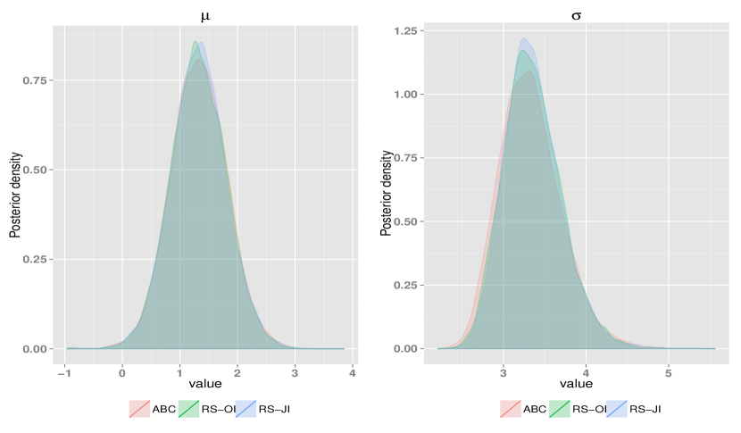
Figure 1: Normally Distributed data

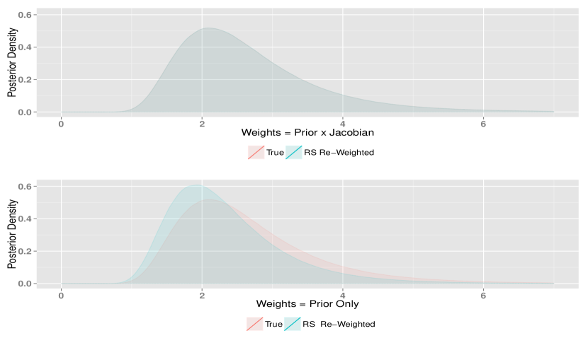
Figure 2: The Importance Weights in RS

To highlight the role of the Jacobian matrix in the RS, the top panel of Figure 2 plots the exact posterior distribution and the one obtained from the reverse sampler. They are indistinguishable. The bottom panel shows an incorrectly constructed reverse sampler that does not apply the Jacobian transformation. Notably, the two distributions are not the same. Re-weighting by the Jacobian matrix is crucial to targeting the desired posterior distribution.

Figure 2 presents the likelihood based posterior distribution, along with the likelihood free ones produced by ABC and the RS-JI (just identified) for one draw of the data. The ABC results are based on the accept-reject algorithm. The numerical results corroborate with the analytical ones: all the posterior distributions are very similar. The RS-JI posterior distribution is very close to the exact posterior distribution. Figure 2 also presents results for the over-identified case (denoted RS-OI) using two additional auxiliary statistics: $\widehat{\bm{\psi}}=(\overline{y},\widehat{\sigma}_{y}^{2},\widehat{\mu}_{3}/\widehat{\sigma}_{y}^{2},\widehat{\mu}_{4}/\widehat{\sigma}_{y}^{4})$ where $\mu_{k}=\mathbb{E}(y^{k})$. The weight matrix is $\text{diag}(1,1,1/2,1/2)$. The posterior distribution is very close to RS-JI obtained for exact identification. We now explain how the posterior distribution for the over-identified case is obtained.

3 The RS: Case $L\geq K$:

The idea behind the RS is the same when we go from the case of exact to overidentification. The precise implementation is as follows. Let $\mathbb{K}_{\delta}(\widehat{\bm{\psi}},\widehat{\bm{\psi}}^{b})$ be a kernel function and $\delta$ be a tolerance level such that $\mathbb{K}_{0}(\widehat{\bm{\psi}},\bm{\psi}^{b})=\mathbbm{I}_{\|\widehat{\bm{\psi}}-\widehat{\bm{\psi}}^{b}\|=0}$.

For $b=1,\ldots,B$

• Generate $\bm{\varepsilon}^{b}$ from $F_{\bm{\varepsilon}}$.

• Find $\bm{\theta}^{b}=\mbox{argmin}_{\bm{\theta}}J^{b}_{1}(\widehat{\bm{\psi}}^{b},\widehat{\bm{\psi}})$ where $\widehat{\bm{\psi}}^{b}=\widehat{\bm{\psi}}(\bm{\theta},\bm{\varepsilon}^{b})$;

• Set $w(\bm{\theta}^{b},\bm{\varepsilon}^{b})=\pi(\bm{\theta}^{b})\text{vol}\left(\widehat{\bm{\psi}}_{\bm{\theta}}^{b}(\bm{\theta}^{b},\bm{\varepsilon}^{b},\widehat{\bm{\psi}})\right)^{-1}\mathbb{K}_{\delta}(J^{b}_{1}(\widehat{\bm{\psi}}^{b},\widehat{\bm{\psi}}))$ where: $\text{vol}(\widehat{\bm{\psi}}^{b}_{\bm{\theta}})=\sqrt{\left|\widehat{\bm{\psi}}_{\bm{\theta}}^{b\prime}\widehat{\bm{\psi}}_{\bm{\theta}}^{b}\right|}.$

• Re-weigh $\bm{\theta}^{b}$ by $\frac{w(\bm{\theta}^{b})}{\sum_{b=1}^{B}w(\bm{\theta}^{b})}$.

We now proceed to explain the two changes:- the use of volume in place of determinant in the importance ratio, and the need for $L-K$ dimensional kernel smoothing.

The usual change of variable formula evaluates the absolute value of the determinant of the Jacobian matrix when the matrix is square. The determinant then gives the infinitesimal dilatation of the volume element in passing from one set of variables to another. The main issue in the case of overidentification is that the determinant of a rectangular Jacobian matrix is not well defined. However, as shown in Ben-Israel (1999), the determinant can be replaced by the volume when transforming from sets of a higher dimension to a lower one. For a $L\times K$ matrix $A$, its volume, denoted $\text{vol}(A),$ is the product of the (non-zero) singular values of $A$:

$$\text{vol}(A)=\begin{cases}\sqrt{|A^{\prime}A}|\quad&L\geq K,\;\;\text{rank}(A)=K\\ \sqrt{|AA^{\prime}|}\quad&L\leq K,\;\;\text{rank}(A)=L.\end{cases}$$

Furthermore, if $A=BC$, $\text{vol}(A)=\text{vol}(B)\text{vol}(C).$

To verify that our target distribution is unaffected by whether we calculate the volume or the determinant of the Jacobian matrix when $K=L$, observe that

$$\widehat{\bm{\psi}}^{b}_{\bm{\theta}}(\bm{\theta}^{b}(\widehat{\bm{\psi}}),\bm{\varepsilon}^{b})=\frac{\partial\widehat{\bm{\psi}}^{b}(\bm{\theta}^{b},\bm{\varepsilon}^{b},\widehat{\bm{\psi}})}{\partial\widehat{\bm{\psi}}}\frac{\partial\widehat{\bm{\psi}}}{\partial\bm{\theta}^{b}}.$$ (5)

The $K$ first order conditions defined by (3) become:

$$\mathcal{F}(\bm{\theta}^{b},\bm{\varepsilon}^{b},\widehat{\bm{\psi}})=\widehat{\bm{\psi}}^{b}_{\bm{\theta}}(\bm{\theta}^{b},\bm{\varepsilon}^{b},\widehat{\bm{\psi}})^{\prime}\mathrm{W}\bigg{(}\widehat{\bm{\psi}}-\widehat{\bm{\psi}}^{b}(\bm{\theta}^{b},\bm{\varepsilon}^{b})\bigg{)}=0.$$ (6)

Since $L=K$, $W$ can be set to an identity matrix $I_{K}$. Furthermore, $\bm{\psi}(\bm{\theta}^{b},\bm{\varepsilon})=\widehat{\bm{\psi}}$ since $J_{1}^{b}(\bm{\theta}^{b})=0$ under exact identification. As $\frac{\partial\bm{\theta}}{\partial\widehat{\bm{\psi}}}$ is a square matrix when $K=L$, we can directly use the fact that $\mathcal{F}_{\bm{\theta}}(\bm{\theta}^{b},\bm{\varepsilon}^{b},\widehat{\bm{\psi}})d\bm{\theta}+\mathcal{F}_{\bm{\psi}}(\bm{\theta}^{b},\bm{\varepsilon}^{b},\widehat{\bm{\psi}})d\widehat{\bm{\psi}}=0$ to obtain the required determinant:

$$|\widehat{\bm{\psi}}^{b}_{\bm{\theta}}(\bm{\theta}^{b},\bm{\varepsilon}^{b},\widehat{\bm{\psi}})|^{-1}=\mathrm{I}_{K}\cdot|\frac{\partial\bm{\theta}}{\partial\widehat{\bm{\psi}}}|=|-\mathcal{F}_{\bm{\theta}}(\bm{\theta}^{b},\bm{\varepsilon}^{b},\widehat{\bm{\psi}})^{-1}\mathcal{F}_{\widehat{\bm{\psi}}}(\bm{\theta}^{b},\bm{\varepsilon}^{b},\widehat{\bm{\psi}})|.$$ (7)

Now to use the volume result, put $\mathrm{A}=\mathrm{I}_{K}$, $\mathrm{B}=\frac{\partial\bm{\theta}}{\partial\widehat{\bm{\psi}}}$ and $\mathrm{C}=\frac{\partial\widehat{\bm{\psi}}}{\partial\bm{\theta}}$. But $\mathrm{A}$ is just a $K$-dimensional identity matrix. Hence $\text{vol}(\mathrm{I}_{K})=\text{vol}\bigg{(}\frac{\partial\bm{\theta}}{\partial\widehat{\bm{\psi}}}\bigg{)}\text{vol}\bigg{(}\frac{\partial\widehat{\bm{\psi}}}{\partial\widehat{\bm{\theta}}}\bigg{)}$ which evaluates to

$$\text{vol}\bigg{(}\frac{\partial\widehat{\bm{\psi}}}{\partial\bm{\theta}}\bigg{)}^{-1}=\text{vol}\bigg{(}\frac{\partial\bm{\theta}}{\partial\widehat{\bm{\psi}}}\bigg{)},\quad\quad\text{or}\quad\quad\bigg{|}\frac{\partial\widehat{\bm{\psi}}}{\partial\bm{\theta}}\bigg{|}^{-1}=\bigg{|}\frac{\partial\bm{\theta}}{\partial\widehat{\bm{\psi}}}\bigg{|}$$

which is precisely $|\widehat{\bm{\psi}}^{b}_{\bm{\theta}}(\bm{\theta},\bm{\varepsilon})|^{-1}$ as given in (7). Hence in the exactly identified case, there is no difference whether one evaluates the determinant or the volume of the Jacobian matrix.

Next, we turn to the role of the kernel function $\mathbb{K}_{\delta}(\widehat{\bm{\psi}},\widehat{\bm{\psi}}^{b})$. The joint density $h(\bm{\theta}^{b},\bm{\varepsilon}^{b})$ is related to $p_{\widehat{\bm{\psi}}^{b},\bm{\varepsilon}^{b}}(\widehat{\bm{\psi}}(\bm{\theta}^{b},\bm{\varepsilon}^{b}))=p(\widehat{\bm{\psi}}^{b},\bm{\varepsilon}^{b})$ through a change a variable now expressed in terms of volume:

$$h(\bm{\theta},\bm{\varepsilon}^{b}|\widehat{\bm{\psi}})=p(\widehat{\bm{\psi}}^{b},\bm{\varepsilon}^{b}|\widehat{\bm{\psi}})\cdot\text{vol}\left(\widehat{\bm{\psi}}_{\bm{\theta}}^{b}(\bm{\theta}^{b},\bm{\varepsilon}^{b},\widehat{\bm{\psi}})\right)$$

When $L\geq K$, the objective function $\|\widehat{\bm{\psi}}-\widehat{\bm{\psi}}^{b}\|_{\mathrm{W}}=J_{1}^{b}\geq 0$ measures the extent to which $\widehat{\bm{\psi}}$ deviates from $\widehat{\bm{\psi}}^{b}$ when the objective function at its minimum. Consider the thought experiment that $J_{1}^{b}=0$ with probability 1, such as enabled by a particular draw of $\bm{\varepsilon}^{b}$. Then the arguments above for $K=L$ would have applied. We would still have $p(\bm{\theta}^{b}|\widehat{\bm{\psi}})=\int\pi(\bm{\theta}^{b})p(\widehat{\bm{\psi}}^{b},\bm{\varepsilon}^{b}|\widehat{\bm{\psi}})\mathbbm{I}_{\|\widehat{\bm{\psi}}-\widehat{\bm{\psi}}^{b}\|=0}d\bm{\varepsilon}^{b}=\int w(\bm{\theta}^{b},\bm{\varepsilon}^{b})h(\bm{\theta}^{b},\bm{\varepsilon}^{b}|\widehat{\bm{\psi}})d\bm{\varepsilon}^{b}$, except that the weights are now defined in terms of volume. Proposition 1 would then extend to the case with $L\geq K$.

But in general $J_{1}^{b}\neq 0$ almost surely. Nonetheless, we can use only those draws that yield $J_{1}^{b}(\bm{\theta}^{b})$ that are sufficiently close to zero. The more draws we make, the tighter this criterion can be. Suppose there is a symmetric kernel $\mathbb{K}_{\delta}(\cdot)$ satisfying conditions in Pagan and Ullah (1999, p.96) for consistent estimation of conditional moments non-parametrically. Analogous to Proposition 1, the volume $\text{vol}\big{(}\widehat{\bm{\psi}}_{\bm{\theta}}^{b}(\bm{\theta}^{b},\bm{\varepsilon}^{b},\widehat{\bm{\psi}})\big{)}$ is assumed to be bounded away from zero. Then as the number of draws $B\rightarrow\infty$, the bandwidth $\delta(B)\rightarrow 0$ and $B\delta(B)\rightarrow\infty$ with

$$w_{\delta(B)}(\bm{\theta}^{b},\widehat{\bm{\varepsilon}}^{b}) = \pi(\bm{\theta}^{b})\text{vol}\bigg{(}\widehat{\bm{\psi}}_{\bm{\theta}}^{b}(\bm{\theta}^{b},\bm{\varepsilon}^{b},\widehat{\bm{\psi}})\bigg{)}^{-1}\mathbb{K}_{\delta(B)}(\widehat{\bm{\psi}},\widehat{\bm{\psi}}^{b}),$$ (8)

a result analogous to Proposition 1 can be obtained:

$$\frac{1}{B}\sum_{b}w_{\delta(B)}(\bm{\theta}^{b},\bm{\varepsilon}^{b})\varphi(\bm{\theta}^{b})\smash{\mathop{\longrightarrow}\limits^{p}}\iint\varphi(\bm{\theta})w_{0}(\bm{\theta},\bm{\varepsilon})\text{vol}\bigg{(}\widehat{\bm{\psi}}^{b}_{\bm{\theta}}(\bm{\theta},\bm{\varepsilon}^{b};\widehat{\bm{\psi}})\bigg{)}p(\widehat{\bm{\psi}},\bm{\varepsilon}^{b}|\bm{\theta})d\bm{\theta}d\bm{\varepsilon}^{b}$$

$$=\iint\varphi(\bm{\theta})\pi(\bm{\theta})\mathbbm{1}_{\|\widehat{\bm{\psi}}-\widehat{\bm{\psi}}^{b}\|=0}\text{vol}\bigg{(}\widehat{\bm{\psi}}^{b}_{\bm{\theta}}(\bm{\theta},\bm{\varepsilon}^{b};\widehat{\bm{\psi}})\bigg{)}^{-1}p(\widehat{\bm{\psi}}^{b},\bm{\varepsilon}^{b}|\bm{\theta})\text{vol}\bigg{(}\widehat{\bm{\psi}}^{b}_{\bm{\theta}}(\bm{\theta},\bm{\varepsilon}^{b};\widehat{\bm{\psi}})\bigg{)}d\bm{\theta}d\bm{\varepsilon}^{b}$$

$$=\iint\varphi(\bm{\theta})\pi(\bm{\theta})1_{\|\widehat{\bm{\psi}}-\widehat{\bm{\psi}}^{b}\|=0}p(\widehat{\bm{\psi}},\bm{\varepsilon}^{b}|\bm{\theta})d\bm{\theta}d\bm{\varepsilon}^{b}$$

$$=\int\varphi(\bm{\theta})\pi(\bm{\theta})L(\widehat{\bm{\psi}}|\bm{\theta})d\bm{\theta}.$$

Similarly, the integrating constant is consistent as $\frac{1}{B}\sum_{b}w_{\delta(B)}(\bm{\theta}^{b},\bm{\varepsilon}^{b})\smash{\mathop{\longrightarrow}\limits^{p}}\int\pi(\bm{\theta})L(\widehat{\bm{\psi}}|\bm{\theta})d\bm{\theta}.$ Hence, the RS sampler still recovers the posterior distribution with the infeasible likelihood. Note that the kernel function was introduced for developing a result analogous to Proposition 1, but no kernel smoothing is required in practical implementation. What is needed for the RS in the over-identified case is $B$ draws with sufficiently small $J_{1}(\bm{\theta}^{b})$. Hence, we can borrow the idea used in the AR-ABC. Specifically, we fix a quantile $q$, repeat $[B/q]$ times until the desired number of draws is obtained. Discarding some draws seems necessary in many ABC implementations.

In summary, there are two changes in implementation of the RS in the over-identified case: the volume and the kernel function. Kernel smoothing has no role in the RS when $K=L$. It is interesting to note that while the ABC and RS both rely on the kernel $\mathbb{K}_{\delta}$ to keep draws close to $\widehat{\bm{\psi}}^{b}$ in the over-identified case, the non-parametric rate at which the sum converges to the integral are different. The RS uses the first order conditions $\widehat{\bm{\psi}}_{\bm{\theta}}^{b}(\bm{\theta}^{b},\bm{\varepsilon}^{b})^{\prime}\mathrm{W}\left(\widehat{\bm{\psi}}^{b}(\bm{\theta}^{b},\bm{\varepsilon}^{b})-\widehat{\bm{\psi}}\right)=0$ to indicate which $K$ combinations of $\widehat{\bm{\psi}}^{b}(\bm{\theta}^{b},\bm{\varepsilon}^{b})-\widehat{\bm{\psi}}$ are set to zero, rendering the dimension of the smoothing problem $L-K$. To see this, note first that each draw $\bm{\theta}^{b}$ from the RS is consistent for $\bm{\theta}_{0}$ and asymptotically normal as shown in Forneron and Ng (2014). In consequence, the first order condition (FOC) can be re-written as: $\left(\frac{d\bm{\psi}(\bm{\theta})}{d\bm{\theta}}\big{|}_{\bm{\theta}=\bm{\theta}_{0}}+O_{p}(\frac{1}{\sqrt{T}})\right)^{\prime}\mathrm{W}\left(\widehat{\bm{\psi}}^{b}(\bm{\theta}^{b},\bm{\varepsilon}^{b})-\widehat{\bm{\psi}}\right)=0$, or

$$\frac{d\bm{\psi}(\bm{\theta})}{d\bm{\theta}}\big{|}_{\bm{\theta}=\bm{\theta}_{0}}^{\prime}\mathrm{W}\left(\widehat{\bm{\psi}}^{b}(\bm{\theta}^{b},\bm{\varepsilon}^{b})-\widehat{\bm{\psi}}\right)=o_{p}(\frac{1}{\sqrt{T}}).$$

Since $\frac{d\bm{\psi}(\bm{\theta})}{d\bm{\theta}}\big{|}_{\bm{\theta}=\bm{\theta}_{0}}^{\prime}\mathrm{W}$ is full rank, there exists a subspace of dimension $K$ such that $\widehat{\bm{\psi}}^{b}(\bm{\theta}^{b},\bm{\varepsilon}^{b})-\widehat{\bm{\psi}}$ is zero asymptotically. Hence the kernel smoothing problem is effectively $L-K$ dimensional. The ABC does not use the FOC. Even in the exactly identified case, the kernel smoothing is a $L=K$ dimensional problem. In general, the convergence rate of the ABC is $L\geq K$, the dimension of $\widehat{\bm{\psi}}$.

The following two examples illustrate the properties of the ABC and RS posterior distributions. The first example uses sufficient statistics and the second example does not. Both the ABC and RS achieve the desired number of draws by setting the quantile, as discussed in Section 2.

Example 4: Exponential Distribution

Let $y_{1},\dots,y_{T}\sim\mathcal{E}(\theta),T=5,\theta_{0}=1/2$. Now $\widehat{\psi}=\overline{y}$ is a sufficient statistic for $y_{1},\dots,y_{T}$. For a flat prior $\pi(\theta)\propto 1_{\theta\geq 0}$ we have:

$$p(\theta|\overline{y})\propto p(\theta|y_{1},\dots,y_{T})=\theta^{T}\exp(-\theta^{T}\overline{y})\sim\Gamma(T+1,T\overline{y})$$

In the just identified case, we let $u^{b}_{t}\sim\mathcal{U}_{[0,1]}$ and $y^{b}_{t}=-\log(1-u^{b}_{t})/\theta^{b}$. This gives:

$$\widehat{\psi}^{b}=\frac{1}{T}\sum_{t=1}^{T}y_{t}^{b}=-\frac{1}{T}\sum_{t=1}^{T}\frac{\log(1-u^{b}_{t})}{\theta^{b}}.$$

Since $\overline{y}^{b}=\overline{y}$, the Jacobian matrix is:

$$\widehat{\psi}_{b}(\theta^{b})=\frac{d\widehat{\psi}^{b}(\theta)}{d\theta}\bigg{|}_{\theta^{b}}=\frac{1}{T}\sum_{t=1}^{T}\frac{\log(1-u^{b}_{t})}{[\theta^{b}]^{2}}=-\frac{\overline{y}}{\theta^{b}}.$$

Hence for a given $T$, the weights are: $w(\theta^{b},u^{b})\propto\mathbbm{I}_{\bm{\theta}^{b}\geq 0}\frac{\theta^{b}}{\overline{y}^{b}}=\frac{\theta^{b}}{\overline{y}}$. We verified that the numerical results agree with this analytical result.

In the over identified case, we consider two moments:

$$\widehat{\bm{\psi}}^{b}=\begin{pmatrix}\overline{y}^{b}\\ \widehat{\sigma}_{y}^{b,2}\end{pmatrix}=\begin{pmatrix}\frac{1}{T}\sum_{t=1}^{T}y_{t}^{b}\\ \frac{1}{T}\sum_{t=1}^{T}(y_{t}^{b})^{2}-(\frac{1}{T}\sum_{t=1}^{T}y_{t}^{b})^{2}\end{pmatrix}.$$

Since $\frac{dy_{t}^{b}}{d\theta}=\frac{\log(1-u_{t}^{b})}{(\theta^{b})^{2}}=-\frac{y_{t}^{b}}{\theta^{b}}$. If $\delta=0$, the Jacobian matrix is

$$\widehat{\bm{\psi}}^{b}_{\theta}=-\begin{pmatrix}\frac{1}{T}\sum_{t=1}^{T}\frac{y_{t}^{b}}{\theta}\\ \frac{2}{\theta^{b}}\frac{1}{T}\sum_{t=1}^{T}(y_{t}^{b})^{2}-\frac{2}{\theta^{b}}\bigg{[}\frac{1}{T}\sum_{t=1}^{T}y_{t}^{b}\bigg{]}^{2}\end{pmatrix}=-\begin{pmatrix}\frac{\overline{y}}{\theta^{b}}\\ \frac{2(\widehat{\sigma}_{y})^{2}}{\theta^{b}}\end{pmatrix}.$$

The volume to be computed is $\text{vol}(\widehat{\bm{\psi}}_{\theta}^{b})=\sqrt{|\widehat{\bm{\psi}}^{b\prime}_{\theta}\widehat{\bm{\psi}}^{b}_{\theta}|}$, as stated in the algorithm. Even if $\mathrm{W}=\mathrm{I}$, the volume is the determinant of $\widehat{\bm{\psi}}_{\theta}^{b}$ in the exactly identified case, plus a term relating to the variance of $y^{b}$. We computed $\widehat{\bm{\psi}}^{b}_{\theta}$ for draws with $J_{1}^{b}\approx 0$ using numerical differentiation and verified that the values are very close to the ones computed analytically for this example.

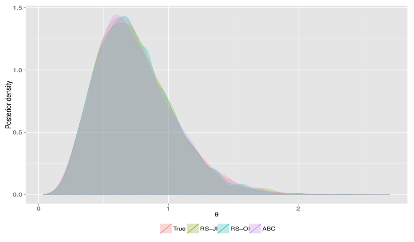
Figure 3: Exponential Distribution

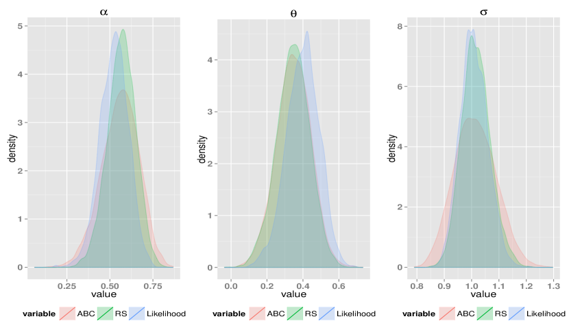
Figure 4: ARMA Model

Figure 4 depicts a particular draw of the ABC posterior distribution (which coincides with the likelihood-based posterior since the statistics are sufficient), along with two generated by the RS sampler. The first one uses the sample mean as auxiliary statistic and hence is exactly identified. The second uses two auxiliary statistics: the sample mean and the sample variance. For the AR-ABC, we draw from the prior ten million times and keep the ten thousand nearest draws. This corresponds to a value of $\delta=0.0135$. For the RS, we draw one million times and keep the ten thousand nearest draws which corresponds to a $\delta=0.0001.$ As for the weight matrix $W$, if we put $W_{11}>0$ and zero elsewhere, we will recover the exactly identified distribution. Here, we intentionally put a positive weight on the variance (which is not a sufficient statistic) to check the effect on the posterior mean. With $\mathrm{W}_{11}=1/5$ and $\mathrm{W}_{22}=4/5$, the RS posterior means are 0.7452 and 0.7456 for the just and overidentifed cases. The corresponding values are are 0.7456 and .7474 for the exact posterior and the ABC-AR. They are very similar.

Example 5: ARMA(1,1):

For $t=1,\ldots,T=200$ and $\bm{\theta}_{0}=(\alpha_{0},\theta_{0},\sigma_{0})=(0.5,0.5,1.0)$, the data are generated as

$$y_{t}=\alpha y_{t-1}+\varepsilon_{t}+\theta\varepsilon_{t-1},\quad\quad\bm{\varepsilon}_{t}\sim\mathcal{N}(0,\sigma^{2}).$$

Least squares estimation of the auxiliary model

$$y_{t}=\phi_{1}y_{t-1}+\phi_{2}y_{t-2}+\phi_{3}y_{t-3}+\phi_{4}y_{t-4}+u_{t}$$

yields $L=5>K=3$ auxiliary parameters

$$\widehat{\bm{\psi}}=(\widehat{\phi}_{1},\widehat{\phi}_{2},\widehat{\phi}_{3},\widehat{\phi}_{4},\widehat{\sigma}_{u}^{2}).$$

We let $\pi(\alpha,\theta,\sigma)=\mathbb{I}_{\alpha,\theta\in[-1,1],\sigma\geq 0}$ and $\mathrm{W}=\mathrm{I}_{5}$ which is inefficient. In this example, $\widehat{\bm{\psi}}$ are not sufficient statistics since $y_{t}$ has an infinite order autoregressive representation.

We draw $\sigma$ from a uniform distribution on $[0,3]$ since $\mathcal{U}_{[0,\infty]}$ is not a proper density. The weights of the RS are obtained by numerical differentiation. The likelihood based posterior is computed by MCMC using the Kalman Filter with initial condition $\varepsilon_{0}=0.$ As mentioned above, the desired number of draws is obtained by setting the quantile instead of setting the tolerance $\delta$. For the RS, we keep the 1/10=10% closest draws corresponding to a $\delta=0.0007$. The Sequential Monte-Carlo implementation of ABC (SMC-ABC) is more efficient at targeting the posterior than the ABC-AR. Hence we also compare the RS with SMC-ABC as implemented in the Easy-ABC package of Lenormand et al. (2013). The requirement for 10,000 posterior draws are as follows:

	AR-ABC	SMC-ABC	RS	Likelihood
Computation Time (hours)	63	25	5	0.1
Effective number of draws	100,000,000	36,805,000	10,153,108
$\delta$	0.0132	0.0283	0.0007

The difference, both in terms of computation time and number of model simulations, is notable. As shown in figure 4 the quality of the approximation is also different, especially for $\alpha$ and $\sigma$. The difference can be traced to $\delta$. The $\delta$ used for the SMC-ABC is effectively much larger than for the RS. A better approximation requires a smaller $\delta$ which implies longer computational time. Alternatively stated, the acceptance rate at a low value of $\delta$ is very low. The caveat is that the speed gain is possible only if the optimization problem can be solved in a few iterations and reasonably fast. In practice, there will be a trade-off between the number of draws and the number of iterations in the optimization step as we further explore below.

4 Acceptance Rate

The RS was initially developed in Forneron and Ng (2014) as a framework to help understand frequentist (SMD) and the Bayesian (ABC) way of likelihood-free estimation. But it turns out that the RS has one computation advantage that is worth highlighting. The issue pertains to the low acceptance rate of the ABC.

As noted above, the ABC exactly recovers the posterior distribution associated with the infeasible likelihood if $\widehat{\bm{\psi}}$ are sufficient statistics and $\delta=0$ as noted in Blum (2010). Of course, $\delta=0$ is an event of measure zero, and the ABC has an approximation bias that depends on $\delta$. In theory, a small $\delta$ is desired. The ABC needs a large number of draws to accurately approximate the posterior and can be computationally costly.

To illustrate this point, consider estimating the mean $m$ in Example 3 with $\sigma^{2}=1$ assumed to be known, and $\pi(m)\propto 1$. All computations are based on the software package R. From a previous draw $m^{b}$, a random walk step gives $m^{\star}=m^{b}+\bm{\varepsilon},\bm{\varepsilon}\sim\mathcal{N}(0,1)$. For small $\delta$, we can assume $m^{\star}|\widehat{m}\sim\mathcal{N}(\widehat{m},1/T)$. From a simulated sample of $T$ observations, we get an estimated mean $\widehat{m}^{\star}\sim\mathcal{N}(m^{\star},1/T)$. As is typical of MCMC chains, these draws are serially correlated. To see that the algorithm can be stuck for a long time if $m^{*}$ is far from $\widehat{m}$, observe that the event $\widehat{m}^{\star}\in[\widehat{m}-\delta,\,\widehat{m}+\delta]$ occurs with probability

$$\mathbb{P}(\widehat{m}^{\star}\in[\widehat{m}-\delta,\,\widehat{m}+\delta])=\Phi\left(\sqrt{T}(\widehat{m}+\delta-m^{\star})\right)-\Phi\left(\sqrt{T}(\widehat{m}-\delta-m^{\star})\right)\approx 2\sqrt{T}\delta\phi\left(\sqrt{T}(\widehat{m}-m^{\star})\right).$$

The acceptance probability $\int_{m^{*}}\mathbb{P}(\widehat{m}^{\star}\in[\widehat{m}-\delta,\,\widehat{m}+\delta])dm^{*}$ is thus approximately linear in $\delta$. To keep the number of accepted draws constant, we need to increase the number of draws as we decrease $\delta$.

This result that the acceptance rate is linear in $\delta$ also applies in the general case. Assume that $\widehat{\bm{\psi}}^{\star}(\bm{\theta}^{\star})\sim\mathcal{N}(\bm{\psi}(\bm{\theta}^{\star}),\Sigma/T)$. We keep the draw if $\|\widehat{\bm{\psi}}-\widehat{\bm{\psi}}^{\star}(\bm{\theta}^{\star})\|\leq\delta$. The probability of this event can be bounded above by $\sum_{j=1}^{K}\mathbb{P}\left(|\widehat{\bm{\psi}}_{j}-\widehat{\bm{\psi}}_{j}^{\star}(\bm{\theta}^{\star})|\leq\delta\right)$ i.e.:

$$\sum_{j=1}^{K}\Phi\left(\frac{\sqrt{T}}{\sigma_{j}}\left(\widehat{\bm{\psi}}_{j}+\delta-\bm{\psi}_{j}(\bm{\theta}^{\star})\right)\right)-\Phi\left(\frac{\sqrt{T}}{\sigma_{j}}\left(\widehat{\bm{\psi}}_{j}-\delta-\bm{\psi}_{j}(\bm{\theta}^{\star})\right)\right)\approx 2\sqrt{T}\delta\sum_{j=1}^{K}\frac{\phi}{\sigma_{j}}\left(\frac{\sqrt{T}}{\sigma_{j}}\left(\widehat{\bm{\psi}}_{j}-\bm{\psi}_{j}(\bm{\theta}^{\star})\right)\right).$$

The acceptance probability is still at best linear in $\delta$. In general we need to increase the number of draws at least as much as $\delta$ declines to keep the number of accepted draws fixed.

Table 2: Acceptance Probability as a function of $\delta$

$\delta$	10	1	0.1	0.01	0.001
$\mathbb{P}(\|\widehat{\bm{\psi}}-\widehat{\bm{\psi}}^{b}\|_{W}\leq\delta)$	0.72171	0.16876	0.00182	0.00002	$<$0.00001

Table 2 shows the acceptance rate for Example 3 for $\bm{\theta}_{0}=(m_{0},\sigma_{0}^{2})=(0,2)$, $T=20$, and weighting matrix $W=\text{diag}(\widehat{\sigma}^{2},2\widehat{\sigma}^{4})/T,\pi(m,\sigma^{2})\propto\mathbbm{I}_{\sigma^{2}\geq 0}$. The results confirm that for small values of $\delta$, the acceptance rate is approximately linear in $\delta$. Even though in theory, the targeted ABC posterior should be closer to the true posterior when $\delta$ is small, this may not be true in practice because of the poor properties of the MCMC chain. At least for this example, the MCMC chain with moderate value of $\delta$ provides a better approximation to the true posterior density.

To overcome the low acceptance rate issue, Beaumont et al. (2002) suggests to use local regression techniques to approximate $\delta=0$ without setting it equal to zero. The convergence rate is then non-parametric. Gao and Hong (2014) analyzes the estimator of Creel and Kristensen (2013) and finds that to compensate for the large variance associated with the kernel smoothing, the number of simulations need to be larger than $T^{K/2}$ to achieve $\sqrt{T}$ convergence, where $K$ is the number of regressors. Other methods that aim to increase the acceptance rate include the ABC-SMC algorithm of Sisson et al. (2007); Sisson and Fan (2011), as well as the adaptive weighting variant due to Bonassi and West (2015), referred to below as SMC-AW. These methods build a sequence of proposals to more efficiently target the posterior. The acceptance rate still declines rapidly with $\delta$, however.

The RS circumvents this problem because each $\bm{\theta}^{b}$ is accepted by virtue of being the solution of an optimization problem, and hence $\widehat{\bm{\psi}}-\widehat{\bm{\psi}}^{b}(\bm{\theta}^{b})$ is the smallest possible. In fact, in the exactly identified case, $\delta=J_{1}^{b}=0$. Furthermore, the sequence of optimizers are independent, and the sampler cannot be stuck. We use two more examples to highlight this feature.

Example 6: Mixture Distribution

Consider the example in Sisson et al. (2007), also considered in Bonassi and West (2015). Let $\pi(\theta)\propto 1_{\theta\in[-10,10]}$ and

$$x|\theta\sim 1/2\mathcal{N}(\theta,1)+1/2\mathcal{N}(\theta,1/100)$$

Suppose we observe one draw $x=0$. Then the true posterior is $\theta|x\sim 1/2\mathcal{N}(0,1)+1/2\mathcal{N}(0,1/100)$ truncated to $[-10,10]$. As in Sisson et al. (2007) and Bonassi and West (2015), we choose three tolerance levels: $(2,0.5,0.025)$ for AR-ABC. Figure 5 shows that the ABC posterior distributions computed using accept-reject sampling with $\delta=0.025$ are similar to the ones using SMC with and without adaptive weighting. The RS posterior distribution is close to both ABC-SMC and ABC-SMC-AW, and all similar to Figure 3 reported in Bonassi and West (2015). However, they are quite different from the AR-ABC with $\delta=2$ and 0.5 are 2, showing that the choice of $\delta$ is important in ABC.

While the SMC, RS, and ABC-AR sampling schemes can produce similar posterior distributions, Table 3 shows that their computational time differ dramatically. The two SMC algorithms need to sample from a multinomial distribution which are evidently more time consuming. When $\delta=0.25$, the AR-ABC posterior distribution is close to the ones produced by the SMC samplers and the RS, but the computational cost is still high. The AR-ABC is computationally efficient when $\delta$ is large, but as seen from Figure 5, the posterior distribution is quite poorly approximated. The RS takes 0.0017 seconds to solve, which is amazingly fast because for this example, the solution is available analytically. No optimization is involved, and there is no need to evaluate the Jacobian because the model is linear. Of course, in cases when the SMD problem is numerically challenging, numerical optimization can be time consuming as well. Our results nonetheless suggest a role for optimization in Bayesian computation; they need not be mutually exclusive. Combining the ideas is an interesting topic for future research.

Table 3: Computation Time (in seconds)

RS	ABC-AR			ABC-SMC
	$\delta$=2	$\delta$=.5	$\delta$=.025	Sisson et-al	Bonassi-West
.0017	0.4973	1.6353	33.8136	190.1510	199.1510

Example 7: Precautionary Savings

The foregoing examples are simple and are serve illustrative purposes. We now consider an example that indeed has an infeasible likelihood. In Deaton (1991), agents maximize expected utility $\mathbb{E}_{0}\left(\sum_{t=0}^{\infty}\beta^{t}u(c_{t})\right)$ subject to the constraint that assets $a_{t+1}=(1+r)(a_{t}+y_{t}-c_{t})$ are bounded below by zero, where $r$ is interest rate, $y$ is income and $c$ consumption. The desire for precautionary saving interacts with borrowing constraints to generate a policy function that is not everywhere concave, but is a piecewise linear when cash-on-hand is below an endogenous threshold. The policy function can only be solved numerically at assumed parameter values. SMD estimation thus consists of solving the model and simulating $S$ auxiliary statistics at each guess $\bm{\theta}$. Michaelides and Ng (2000) evaluate the finite sample properties of several SMD estimators using a model with similar features. Since the likelihood for this model is not available analytically. Hence Bayesian estimation of this model has not been implemented. Here, we use the RS to approximate the posterior distribution.

We generate $T=400$ observations assuming that $U(c)=\frac{c^{1-\gamma}-1}{1-\gamma}$, $y_{t}\sim\text{ iid }\mathcal{N}(\mu,\sigma^{2})$ with $r=0.05$, $\beta=10/11$, $\mu=100,\sigma=10,\gamma=2$ as true values. We estimate $\bm{\theta}=(\gamma,\mu,\sigma)$ and assume $(\beta,r)$ are known. We use 10 auxiliary statistics:

$$\widehat{\bm{\psi}}=\begin{pmatrix}\overline{y}&\widehat{\Gamma}_{yy}(0)&\widehat{\Gamma}_{aa}(0)&\widehat{\Gamma}_{cc}(0)&\widehat{\Gamma}_{cc}(1)&\widehat{\Gamma}_{aa}(1)&\widehat{\Gamma}_{cc}(2)&\widehat{\Gamma}_{aa}(2)&\widehat{\Gamma}_{cy}(0)&\widehat{\Gamma}_{ay}(0)\end{pmatrix}^{\prime}$$

where $\widehat{\Gamma}_{ab}(j)=\frac{1}{T}\sum_{t=1}^{T}(a_{t}-\overline{a})(b_{t-j}-\overline{b})$. We generate $B=13,423$ draws and keep the $3,356$ (25%) nearest draws to $\widehat{\bm{\psi}}.$ After weighting using the volume of the Jacobian matrix we have an effective sample size of $1,421$ draws. We use an identity weighting matrix so $J_{RS}(\bm{\theta})=\overline{g}(\bm{\theta})^{\prime}\overline{g}(\bm{\theta})$. The Jacobian is computed using finite differences for the RS. As benchmark, we also compute an SMD with $S=100$, $J_{S}=\overline{g}_{S}(\bm{\theta})^{\prime}\overline{g}_{S}(\bm{\theta})$. In this exercise, the SMD only needs to solve for the policy function once at each step of the optimization. Hence the binding function can be approximated using simulated data at a low cost. For this example, the programs are coded in python. The Nelder-Mead method is used for optimization.

Table 4: Deaton Model: RS, SMD with $\mathrm{W}=\mathrm{I}$

	Posterior Mean/Estimate			Posterior SD/SE
	$\gamma$	$\mu$	$\sigma$	$\gamma$	$\mu$	$\sigma$
RS	1.86	99.92	10.48	0.19	0.84	0.37
SMD	1.76	99.38	10.31	0.12	0.60	0.34

Figure 6 shows the posterior distribution of the RS (blue) along with the SMD distribution (purple) as approximated by $\mathcal{N}(\widehat{\bm{\theta}}_{\text{SMD}},\widehat{\mathrm{V}}_{\text{SMD}}/T)$ according to asymptotic theory. Table 4 shows that the two sets of point estimates are similar. As explained in Forneron and Ng (2014), the SMD uses simulations to approximate the binding function while the RS (and by implication the ABC) uses simulations to approximate the infeasible posterior distribution. In this example, the difference in bias is quite small. We should note that the RS took well over a day to solve while the SMD took less than three hours to compute. Whether we use our own code for the ABC-MCMC or from packages available, the acceptance rate is too low for the exercise to be feasible.

5 Conclusion

This paper studies properties of the reverse sampler considered in Forneron and Ng (2014) for likelihood-free estimation. The sampler produce draws from the infeasible posterior distribution by solving a sequence of frequentist SMD problems. We showed that the reverse sampler uses the Jacobian matrix as importance ratio. In the over-identified case, the importance ratio can be computed using the volume of the Jacobian matrix. The reverse sampler does not suffer from the problem of low acceptance rate that makes the ABC computationally demanding.

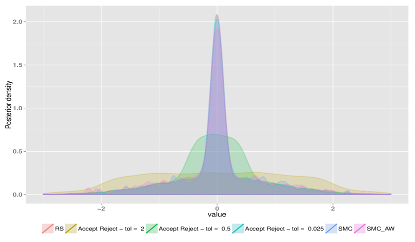
Figure 5: Mixture Distribution

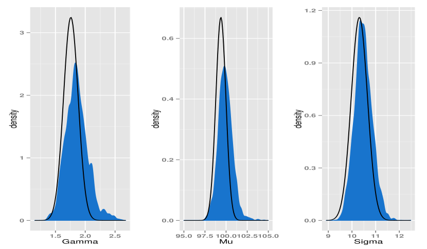
Figure 6: Deaton Model: RS and SMD

Note: Blue density: RS posterior, Black line: large sample approximation for the SMD estimator (identity weighting matrix).

References

- (1)
- Bao and Ullah (2007) Bao, Y. and Ullah, A. 2007, The Second-Order Bias and Mean-Squared Error of Estimators in Time Series Models, Journal of Econometrics 140(2), 650–669.
- Beaumont et al. (2009) Beaumont, M., Corneut, J., Marin, J. and Robert, C. 2009, Adaptive Approximate Bayesian Computation, Biometrika 96(4), 983–990.
- Beaumont et al. (2002) Beaumont, M., Zhang, W. and Balding, D. 2002, Approximate Bayesian Computation in Population Genetics, Genetics 162, 2025–2035.
- Ben-Israel (1999) Ben-Israel, A. 1999, The Change of Variables Forumla Using Matrix Volume, SIAM Journal of Matrix Analysis 21, 300–312.
- Ben-Israel (2001) Ben-Israel, A. 2001, An Application of the Matrix Volume in Probability, Linear Algebra and Applications 321, 9–25.
- Blum (2010) Blum, M. 2010, Approximate Bayesian Computation: A Nonparametric Perspective, Journal of the American Statistical Association 105(491), 1178–1187.
- Bonassi and West (2015) Bonassi, F. and West, M. 2015, Sequential Monte Carlo With Adaptive Weights for Approximate Bayesian Computation, Bayesian Analysis 10(1), 171–187.
- Creel and Kristensen (2013) Creel, M. and Kristensen, D. 2013, Indirect Likelihood Inference, mimeo, UCL.
- Creel and Kristensen (2015) Creel, M. and Kristensen, D. 2015, On Selection of Statistics for Approximate Bayesian Computing or the Method of Simulated Moments, Computational Statistics and Data Analysis.
- Deaton (1991) Deaton, A. S. 1991, Saving and Liqudity Constraints, Econometrica 59, 1221–1248.
- Duffie and Singleton (1993) Duffie, D. and Singleton, K. 1993, Simulated Moments Estimation of Markov Models of Asset Prices, Econometrica 61, 929–952.
- Forneron and Ng (2014) Forneron, J. J. and Ng, S. 2014, The ABC of Simulation Estimation with Auxiliary Statistics, arXiv:1501.01265.
- Gallant and Tauchen (1996) Gallant, R. and Tauchen, G. 1996, Which Moments to Match, Econometric Theory 12, 657–681.
- Gao and Hong (2014) Gao, J. and Hong, H. 2014, A Computational Implementation of GMM, SSRN Working Paper 2503199.
- Gourieroux et al. (1993) Gourieroux, C., Monfort, A. and Renault, E. 1993, Indirect Inference, Journal of Applied Econometrics 85, 85–118.
- Jiang and Turnbull (2004) Jiang, W. and Turnbull, B. 2004, The Indirect Method: Inference Based on Intermediate Statistics- A Synthesis and Examples, Statistical Science 19(2), 239–263.
- Lenormand et al. (2013) Lenormand, M., Jabot, F. and Deffuant, G. 2013, Adaptive Approximate Bayesian Computation Computation for Complex Models, Journal of Computational and Graphical Statistics 28(6), 2777–2796.
- Marjoram et al. (2003) Marjoram, P., Molitor, J., Plagnol, V. and Tavare, S. 2003, Markov Chain Monte Carlo Without Likelihoods, Procedings of the National Academy of Science 100(26), 15324–15328.
- Meeds and Welling (2015) Meeds, E. and Welling, M. 2015, Optimization Monte Carlo: Efficient and Embarrassingly Parallel Likelihood-Free Inference, arXiv:1506:03693v1.
- Michaelides and Ng (2000) Michaelides, A. and Ng, S. 2000, Estimating the Rational Expectations Model of Speculative Storage: A Monte Carlo Comparison of Three Simulation Estimators, Journal of Econometrics 96:2, 231–266.
- Newey and McFadden (1994) Newey, W. and McFadden, D. 1994, Large Sample Estimation and Hypothesis Testing, Handbook of Econometrics, Vol. 36:4, North Holland, pp. 2111–2234.
- Pagan and Ullah (1999) Pagan, A. and Ullah, A. 1999, Nonparametric Econometrics, Vol. Themes in Modern Econometrics, Cambridge University Press.
- Pritchard et al. (1996) Pritchard, J., Seielstad, M., Perez-Lezman, A. and Feldman, M. 1996, Population Growth of Human Y chromosomes: A Study of Y Chromosome MicroSatellites, Molecular Biology and Evolution 16(12), 1791–1798.
- Rilstone et al. (1996) Rilstone, P., Srivastara, K. and Ullah, A. 1996, The Second-Order Bias and Mean Squared Error of Nonlinear Estimators, Journal of Econometrics 75, 369–385.
- Sisson and Fan (2011) Sisson, S. and Fan, Y. 2011, Likelihood Free Markov Chain Monte Carlo, in S. Brooks, A. Celman, G. Jones and X.-L. Meng (eds), Handbook of Markov Chain Monte Carlo, Vol. Chapter 12, pp. 313–335. arXiv:10001.2058v1.
- Sisson et al. (2007) Sisson, S., Fan, Y. and Tanaka, M. 2007, Sequential Monte Carlo Without Likelihood, Procedings of the National Academy of Science 104(6), 1760–1765.
- Smith (1993) Smith, A. 1993, Estimating Nonlinear Time Series Models Using Simulated Vector Autoregressions, Journal of Applied Econometrics 8, S63–S84.
- Tavare et al. (1997) Tavare, S., Balding, J., Griffiths, C. and Donnelly, P. 1997, Inferring Coalescence Times From DNA Sequence Data, Genetics 145, 505–518.
- Toni et al. (2009) Toni, T., Welch, D., Strelkowa, N., Ipsen, A. and Stumpf, M. 2009, Approximate Bayesian Computation Scheme for Parameter Inference and Model Selection in Dynamic Models, Journal of the Royal Society Inference 6, 187–222.
- Vo et al. (2015) Vo, R., Drovandi, C., Pettitt, A. and Pettet, G. 2015, Melanoma Cell Colony Expansion Parameters Revealed by Approximate Bayesian Computation, eprints.qut.edu/au/83824.