Single Top and Higgs Production in $e^{-}p$ collisions

Abstract

In this proceedings some studies on the prospects of single top production at the Large Hadron Electron Collider (LHeC) and double Higgs production at the Future Circular Hadron Electron Collider (FCC-he) shall be presented. In particular, we investigated the $tbW$ couplings via single top quark production with the introduction of possible anomalous Lorentz structures, and measured the sensitivity of the Higgs self coupling ($\lambda$) through double Higgs production. The studies are performed with 60 GeV electrons colliding with 7 (50) TeV protons for the LHeC (FCC-he).

For the single top studies a parton level study has been performed, and we find the sensitivity of the anomalous coupling at a 95% C.L, considering 10-1% systematic errors. The double Higgs production has been studied with speculated detector parameters and the sensitivity of $\lambda$ estimated via the cross section study around the Standard Model Higgs self coupling strength ($\lambda_{SM}$) considering 5% systematic error in signal and backgrounds. Effects of non-standard CP-even and CP-odd couplings for $hhh$, $hWW$ and $hhWW$ vertices have been studied and constrained at 95% C.L.

WITS-MITP-012

1 Introduction

In the Standard Model (SM) of particle physics the top quark, the heaviest among all matter particles, and the Higgs boson, a particle responsible for giving masses to all matter particles and gauge bosons, play a crucial role in the model. And hence it has been, and still is, a challenge for colliders to study different characteristics of these two particles. These characteristics include their charge, mass, interactions and coupling strengths with other particles etc.

As such we shall briefly review some of the important properties of the top quark and the Higgs boson from theoretical calculations and results from present and past colliders. We will then present some predictions for a future $e^{-}p$ collider known as the Large Hadron Electron Collider (LHeC) and the Future Circular Hadron Electron Collider (FCC-he) at a center of mass energy $\sqrt{s}\approx 1.3$ TeV and $\sqrt{s}\approx 3.5$ TeV, respectively.

The structure of this proceeding shall then be: section 2 is devoted to the top quark studies, sections 3 and 4 are devoted for the Higgs boson studies in $e^{-}p$ collisions. We conclude our inferences based on our studies in section 5.

2 The top quark at the LHeC

In this section we briefly review the physics potential of the proposed LHeC by estimating the accuracy of anomalous $Wtb$ couplings in the single anti-top quark production through $e^{-}p$ collisions [1]. Within the SM the $Wtb$ vertex is purely left-handed. However, the most general lowest dimension CP conserving (in effect of which the couplings are real) Lagrangian for this vertex is given by

$${\cal L}_{Wtb}=\frac{g}{\sqrt{2}}\left[W_{\mu}\bar{t}\gamma^{\mu}\left(V_{tb}f_{1}^{L}P_{L}+f_{1}^{R}P_{R}\right)b-\frac{1}{2m_{W}}W_{\mu\nu}\bar{t}\sigma^{\mu\nu}\left(f_{2}^{L}P_{L}+f_{2}^{R}P_{R}\right)b\right]+{\rm h.c}.$$ (1)

Here $f_{1}^{L}=1+\Delta f_{1}^{L}$, $W_{\mu\nu}=\partial_{\mu}W_{\nu}-\partial_{\nu}W_{\mu}$, $P_{L,R}=\frac{1}{2}\left(1\mp\gamma_{5}\right)$ are left- and right-handed projection operators, $\sigma^{\mu\nu}={\rm i}\left(\gamma^{\mu}\gamma^{\nu}-\gamma^{\nu}\gamma^{\mu}\right)/2$ and $g=e/{\sin\theta_{W}}$. In the SM $\left|V_{tb}\right|f_{1}^{L}\approx 1$. So, along with $\Delta f_{1}^{L}$ all other couplings $f_{2}^{L},f_{1}^{R},f_{2}^{R}$ vanish at tree-level, but are non-zero at higher orders. The constraints on these couplings are the following:

• Assuming only one anomalous coupling to be non-zero at a time: $-0.13\leq|V_{tb}|f_{1}^{L}\leq 0.03$, $-0.0007\leq f_{1}^{R}\leq 0.0025$, $-0.0015\leq f_{2}^{L}\leq 0.0004$, $-0.15\leq f_{2}^{R}\leq 0.57$ from $B$ decays;

• Single top production at DØ  assuming $|V_{tb}|f_{1}^{L}=1$: $|f_{1}^{R}|\leq 0.548$, $|f_{2}^{L}|\leq 0.224$, $|f_{2}^{R}|\leq 0.347$;

• Associated $tW$ production at LHC through $\gamma p$ collision: $|f_{1}^{R}|\leq 0.55$, $|f_{2}^{L}|\leq 0.22$, $|f_{2}^{R}|\leq 0.35$;

• ATLAS: asymmetries associated through angular distribution Re$\left(f_{1}^{R}\right)\in$ [-0.44,0.48], Re$\left(f_{2}^{L}\right)\in$ [-0.24,0.21], Re$\left(f_{2}^{R}\right)\in$ [-0.49,0.15].

Loop Corrections:

• QCD: $f_{2}^{R}=-6.61\times 10^{-3}$, $f_{2}^{L}=-1.118\times 10^{-3}$ ($m_{t}=171$ GeV);

• EW: $f_{2}^{R}=-(1.24\pm 1.23{\rm i})\times 10^{-3}$, $f_{2}^{L}=-(0.102\pm 0.014{\rm i})\times 10^{-3}$ ($m_{h}=126$ GeV);

• SM: $f_{2}^{R}=-(7.85\pm 1.23{\rm i})\times 10^{-3}$, $f_{2}^{L}=-(1.220\pm 0.014{\rm i})\times 10^{-3}$.

2.1 Single anti-top production

We analyze the anti-top production through the hadronic and leptonic decay modes of $W$’s as (a) $e^{-}p\to\bar{t}\nu_{e},\left(\bar{t}\to W^{-}\bar{b},W^{-}\to jj\right)$ and (b) $e^{-}p\to\bar{t}\nu_{e},\left(\bar{t}\to W^{-}\bar{b},W^{-}\to l\nu_{l}\right)$, respectively. We impose the following selection cuts on events:

• Minimum transverse momenta: $p_{T_{b,j}}\geq 20$ GeV, $p_{T_{b,\bar{l}}}\geq 25$ GeV and $\not{E}_{T}\geq 25$ GeV;

• Pseudorapidities: $\left|\eta_{\bar{b},l}\right|\leq 2.5$ and $\left|\eta_{j}\right|\leq 2.5$;

• Isolation cuts: $\Delta R_{ij}\geq 0.4$ where $i,j$ are leptons, light-jets and $b$-jets;

• $\Delta\phi_{\not{E}_{T},j}>$ 0.4, $\Delta\phi_{\not{E}_{T},l}>$ 0.4, $\Delta\phi_{\not{E}_{T},b}>$ 0.4 and

• $\left|m_{j_{1}j_{2}}-m_{W}\right|\leq 22$ GeV for the hadronic channel.

After estimation of all possible backgrounds in both channels, imposing the above selection cuts, we observed high yields of single anti-top quark production with fiducial efficiency of $\sim 70$ % and $\sim 90$ % in the hadronic and leptonic decay modes of $W^{-}$ respectively.

2.2 Estimators and $\chi^{2}$ analysis

To find the sensitivity of all non-standard couplings, we follow three different approaches based on one dimensional histograms. In the histograms we compare the SM distributions, including all backgrounds, with all non-standard couplings with representative values $f_{1}^{R}=+0.5$, $f_{2}^{L}=-0.5$, $f_{2}^{L}=+0.5$ and $f_{2}^{R}=+0.5$. For hadronic modes, we consider six different distributions, namely, $\Delta\phi_{E_{T}^{miss}j_{1}}$, $\Delta\phi_{E_{T}^{miss}b}$, $\Delta\phi_{E_{T}^{miss}W}$, $\Delta\phi_{bW}$, $\cos\theta_{bj_{1}}$ and $\Delta\eta_{bj_{1}}$, while for leptonic modes, there are four different one dimensional histograms used for the analysis $\Delta\phi_{E_{T}^{miss}l}$, $\Delta\phi_{E_{T}^{miss}b}$, $\cos\theta_{bl}$ and $\Delta\eta_{bl}$.

2.2.1 Angular Asymmetries from Histograms:

As a preliminary study in order to get a feel for different chiral and momentum dependencies of couplings, the following asymmetries are defined:

$$A_{\theta_{ij}} =\,\frac{N_{+}^{A}(\cos\theta_{ij}>0)-N_{-}^{A}(\cos\theta_{ij}<0)}{N_{+}^{A}(\cos\theta_{ij}>0)+N_{-}^{A}(\cos\theta_{ij}<0)},$$ (2)

$$A_{\Delta\eta_{ij}} =\,\frac{N_{+}^{A}(\Delta\eta_{ij}>0)-N_{-}^{A}(\Delta\eta_{ij}<0)}{N_{+}^{A}(\Delta\eta_{ij}>0)+N_{-}^{A}(\Delta\eta_{ij}<0)},$$ (3)

$$A_{\Delta\Phi_{ij}} =\,\frac{N_{+}^{A}\left(\Delta\phi_{ij}>\frac{\pi}{2}\right)-N_{-}^{A}\left(\Delta\phi_{ij}<\frac{\pi}{2}\right)}{N_{+}^{A}\left(\Delta\phi_{ij}>\frac{\pi}{2}\right)+N_{-}^{A}\left(\Delta\phi_{ij}<\frac{\pi}{2}\right)},$$ (4)

with $0\leq\Delta\phi_{ij}\leq\pi$. The asymmetry $A_{\alpha}$ and its statistical error for $N_{+}^{A}$ and $N_{-}^{A}$ events, where $N=\left(N_{+}^{A}+N_{-}^{A}\right)=L\cdot\sigma$, are calculated using the following definition based on binomial distributions:

$$A_{\alpha} = a\pm\sigma_{a},\qquad{\rm where}$$ (5)

$$a = \frac{N_{+}^{A}-N_{-}^{A}}{N_{+}^{A}+N_{-}^{A}}\quad{\rm and}\quad\sigma_{a}=\sqrt{\frac{1-a^{2}}{L\cdot\sigma}}\,;\quad\left(\alpha=\cos\theta_{ij},\Delta\eta_{ij},\Delta\Phi_{ij}\right).$$ (6)

Here $\sigma\equiv\sigma(e^{-}p\to\bar{t}\nu,\,\bar{t}\to W^{-}\bar{b})\times BR(W^{-}\to jj/\,l^{-}\bar{\nu})\times\epsilon_{b}$ is the total cross section in the respective channels after imposing selection cuts and $\epsilon_{b}=0.6$ is the $b/\bar{b}$ tagging efficiency.

	$A_{\Delta\Phi_{\not{E}_{T}j_{1}}}$	$A_{\Delta\Phi_{\not{E}_{T}\bar{b}}}$	$A_{\Delta\Phi_{\not{E}_{T}W^{-}}}$	$A_{\Delta\Phi_{W^{-}\bar{b}}}$	$A_{\theta_{\bar{b}j_{1}}}$	$A_{\Delta\eta_{\bar{b}j_{1}}}$
SM+$\sum_{i}{\rm Bkg}_{i}$	.532 $\pm$ .003	.282 $\pm$ .005	.503 $\pm$ .004	.799 $\pm$ .003	.023 $\pm$ .001	-.712 $\pm$ .003
$f_{1}^{R}=+.5$	.327 $\pm$ .004	.231 $\pm$ .004	.564 $\pm$ .004	.778 $\pm$ .003	.0005 $\pm$ .004	-.806 $\pm$ .003
$f_{2}^{L}=-.5$	.528 $\pm$ .004	.082 $\pm$ .004	.716 $\pm$ .003	.748 $\pm$ .003	-.196 $\pm$ .004	-.868 $\pm$ .002
$f_{2}^{L}=+.5$	.390 $\pm$ .005	.269 $\pm$ .004	.585 $\pm$ .004	.683 $\pm$ .004	.106 $\pm$ .005	-.795 $\pm$ .003
$f_{2}^{R}=+.5$	.330 $\pm$ .004	.363 $\pm$ .004	.566 $\pm$ .003	.656 $\pm$ .003	-.197 $\pm$ .004	-.823 $\pm$ .002

Table 1: Asymmetries and errors associated with the kinematic distributions in hadronic histograms at an integrated luminosity $L$ = 100 fb^-1.

	$A_{\Delta\Phi_{\not{E}_{T}l_{1}}}$	$A_{\Delta\Phi_{\not{E}_{T}\bar{b}}}$	$A_{\theta_{\bar{b}l_{1}}}$	$A_{\Delta\eta_{\bar{b}l_{1}}}$
SM + $\sum_{i}{\rm Bkg}_{i}$	.384 $\pm$ .004	.710 $\pm$ .003	.551 $\pm$ .006	-.765 $\pm$ .007
$f_{1}^{R}=+.5$	.484 $\pm$ .004	.702 $\pm$ .003	.332 $\pm$ .006	-.821 $\pm$ .003
$f_{2}^{L}=-.5$	.526 $\pm$ .004	.620 $\pm$ .003	.410 $\pm$ .006	-.831 $\pm$ .002
$f_{2}^{L}=+.5$	.353 $\pm$ .005	.812 $\pm$ .003	.392 $\pm$ .007	-.850 $\pm$ .003
$f_{2}^{R}=+.5$	.424 $\pm$ .004	.684 $\pm$ .003	.507 $\pm$ .005	-.809 $\pm$ .003

Table 2: Asymmetries and errors associated with the kinematic distributions in leptonic histograms at an integrated luminosity $L$ = 100 fb^-1.

Tables 1 and 2 show how asymmetries are affected due to anomalous couplings of the order $10^{-1}$. The asymmetry suggests that the distribution of the cosine of the angle between the tagged $\bar{b}$ quark and the highest $p_{T}$ jet $j_{1}$ in the hadronic mode is the most sensitive observable.

2.2.2 Exclusion contour from bin analysis:

To make the analysis more effective we perform the $\chi^{2}$ analysis defined as:

$$\chi^{2}\left(f_{i},f_{j}\right) = \sum_{k=1}^{N}\,\left(\,\frac{{\cal N}^{\rm exp}_{k}-{\cal N}^{\rm th}_{k}\left(f_{i},f_{j}\right)}{\delta{\cal N}^{\rm exp}_{k}}\,\right)^{2},$$ (7)

where ${\cal N}_{k}^{\rm th}\left(f_{i},f_{j}\right)$ and ${\cal N}_{k}^{\rm exp}$ are the total number of events predicted by the theory involving $f_{i},\,f_{j}$ and measured in the experiment for the $k^{\rm th}$ bin. $\delta{\cal N}_{k}^{\rm exp}$ is the combined statistical and systematic error $\delta_{\rm sys}$ in measuring the events for the $k^{\rm th}$ bin. If all the coefficient $f_{i}$’s are small, then the experimental result in the $k^{\rm th}$ bin should be approximated by the SM and background prediction as

$${\cal N}^{\rm exp}_{k}\approx{\cal N}^{\rm SM}_{k}+\sum_{i}{\cal N}^{\rm Bkg_{i}}_{k}={\cal N}^{\rm SM+\sum_{i}Bkg_{i}}_{k}.$$ (8)

The error $\delta{\cal N}_{k}^{\rm SM}$ can be defined as

$$\delta{\cal N}_{k}^{\rm SM+\sum Bkg_{i}}=\sqrt{{\cal N}_{k}^{\rm SM+\sum_{i}Bkg_{i}}\left(1+\delta_{\rm sys}^{2}\,\,{\cal N}_{k}^{\rm SM+\sum_{i}Bkg_{i}}\right)}.$$ (9)

The $\chi^{2}$ analysis due to un-correlated systematic uncertainties is studied for three representative values of $\delta_{\rm sys}$ at 1%, 5% and 10 %, respectively. And the sensitivity of $\left|V_{tb}\right|\Delta f_{1}^{L}$ at 95% C.L. is found to be of the order of $\sim 10^{-3}-10^{-2}$ with the corresponding variation of 1% - 10% in the systematic error (which includes the luminosity error). The order of the sensitivity for other anomalous couplings varies between $\sim 10^{-2}-10^{-1}$ at 95 % C.L.

2.2.3 Errors and correlations:

Further, defining the combined $\chi^{2}_{comb.}\left(f_{i},f_{j}\right)$ and taking into account of luminosity error $L\equiv\beta\bar{L},\beta=1\pm\Delta\beta$:

$$\chi^{2}_{\rm comb.}(f_{i},f_{j})\rightarrow\chi^{2}_{\rm comb.}(f_{i},f_{j},\,\beta)\equiv\sum_{k=1}^{m}\sum_{i=0}^{n}\sum_{j=0}^{n}(f_{i}-\bar{f_{i}})\left[V^{-1}\right]_{ij}^{k}(f_{j}-\bar{f_{j}})+\left(\frac{\beta_{k}-1}{\Delta\beta_{k}}\right)^{2},$$ (10)

the sensitivity of $\left|V_{tb}\right|\Delta f_{1}^{L}\sim 10^{-2}$ and for other couplings it is $\sim 10^{-4}$ for $\Delta\beta\geq 5\%$.

Our analysis shows that the anomalous $Wtb$ vertex at the LHeC can be probed to a very high accuracy in comparison to all existing limits.

3 The Higgs boson at the LHeC

As mentioned in the introduction, the Higgs boson searches are of utmost importance for all past and present colliders. However, some properties need to be measured accurately and in this respect future colliders also play a very important role. In Ref. [2] the authors studied the $hb\bar{b}$ coupling at the LHeC, and they demonstrated that the requirement of forward jet tagging in charged current events strongly enhances the signal-to-background ratio. The charged current process at the LHeC is $W$-vector boson fusion and hence one could measure $hWW$ coupling strength as well. CP properties of the Higgs boson can be determined by considering an effective five-dimensional vertex, given as [3],

$$\Gamma_{\mu\nu}\left(p,q\right)=\frac{g}{M_{W}}\left[\lambda\left(p\cdot qg_{\mu\nu}-p_{\nu}q_{\mu}\right)+i\lambda^{\prime}\epsilon_{\mu\nu\rho\sigma}p^{\rho}q^{\sigma}\right],$$ (11)

where $\lambda$ and $\lambda^{\prime}$ are the effective coupling strengths for the anomalous CP-conserving and the CP-violating operators, respectively. They have shown that the azimuthal angle between missing energy and non-$b$ jet $\Delta\phi_{MET-J}$ is a powerful and unambiguous probe of anomalous $hWW$ couplings, both for CP-conserving and violating type.

4 Double Higgs boson production at the FCC-he

Further plans for a high-energy LHC provides 50 TeV protons and hence the LHeC center of mass energy could be increased up to $\sim 3.5$ TeV with 60 GeV electrons, named as the FCC-he. This energy provides opportunities to probe the Higgs self coupling strength $g^{(1)}_{hhh}$ through double Higgs boson production. In this work we consider the speculated detector parameters and cut-based analysis to get charged-current signals with respect to all possible charged/neutral-current and photo-production backgrounds [4]. A statistical analysis is also performed to find the sensitivity of $g^{(1)}_{hhh}$ with other effective couplings described with the following effective Lagrangian:

$${\cal L}^{(3)}_{hhh}= \,\frac{m^{2}_{h}}{2v}(1-g^{(1)}_{hhh})h^{3}+\frac{1}{2}g^{(2)}_{hhh}h\partial_{\mu}h\partial^{\mu}h,$$ (12)

$${\cal L}^{(3)}_{hWW}= -\frac{g}{2m_{W}}g^{(1)}_{hWW}W^{\mu\nu}W^{\dagger}_{\mu\nu}h-\frac{g}{m_{W}}\left[g^{(2)}_{hWW}W^{\nu}\partial^{\mu}W^{\dagger}_{\mu\nu}h+{\rm h.c.}\right]$$

$$-\frac{g}{2m_{W}}\tilde{g}_{hWW}W^{\mu\nu}\tilde{W}^{\dagger}_{\mu\nu}h,$$ (13)

$${\cal L}^{(4)}_{hhWW}= -\frac{g^{2}}{4m^{2}_{W}}g^{(1)}_{hhWW}W^{\mu\nu}W^{\dagger}_{\mu\nu}h^{2}-\frac{g^{2}}{2m^{2}_{W}}\left[g^{(2)}_{hhWW}W^{\nu}\partial^{\mu}W^{\dagger}_{\mu\nu}h^{2}+{\rm h.c.}\right]$$

$$-\frac{g^{2}}{4m^{2}_{W}}\tilde{g}_{hhWW}W^{\mu\nu}\tilde{W}^{\dagger}_{\mu\nu}h^{2}.$$ (14)

Here $g^{(1)}_{hhh}$ is defined such that it appears as a multiplicative constant to $\lambda_{SM}$ i.e; $\lambda\to g^{(1)}_{hhh}\lambda_{SM}$ in the potential for electroweak symmetry breaking in the SM:

$$V(\Phi)=\mu^{2}\Phi^{\dagger}\Phi+\lambda(\Phi^{\dagger}\Phi)^{2}\to\frac{1}{2}m^{2}_{h}h^{2}+\lambda vh^{3}+\frac{\lambda}{4}h^{4},$$ (15)

with $\lambda=\lambda_{\rm SM}=m^{2}_{h}/(2v^{2})\approx 0.13$. The effective couplings $g^{(1)}_{hhh}$, $g^{(2)}_{hhh}$, $g^{(1)}_{hWW}$, $g^{(2)}_{hWW}$, $g^{(1)}_{hhWW}$, and $g^{(2)}_{hhWW}$ are CP-conserving, whereas $\tilde{g}_{hWW}$, $\tilde{g}_{hhWW}$ are CP-violating effective couplings. $m_{h}$ and $m_{W}$ are respectively masses of the Higgs and $W$-bosons, $W^{\mu\nu}=\partial^{\mu}W^{\nu}-\partial^{\nu}W^{\mu}$.

4.1 Cross section, Detector setup and cut-based analysis

Fiducial cross sections for signal and backgrounds, before cut-based analysis, are shown in Table 3. For signal we consider the charged current process $pe^{-}\to\nu_{e}hhj,h\to b\bar{b}$. Photo-production backgrounds are very important for signals, other charged/neutral-current backgrounds, and those backgrounds estimated through “Equivalent photon approximation structure functions”; which is calculated with the “Improved Weizsaecker-Williams formula” [5].

Process	cc (fb)	nc (fb)	photo (fb)
Signal:	$2.40\times 10^{-1}$	$3.95\times 10^{-2}$	$3.30\times 10^{-6}$
$b\bar{b}b\bar{b}j$:	$8.20\times 10^{-1}$	$3.60\times 10^{+3}$	$2.85\times 10^{+3}$
$b\bar{b}jjj$:	$6.50\times 10^{+3}$	$2.50\times 10^{+4}$	$1.94\times 10^{+6}$
$zzj$($z\to b\bar{b}$):	$7.40\times 10^{-1}$	$1.65\times 10^{-2}$	$1.73\times 10^{-2}$
$t\bar{t}j$(hadronic):	$3.30\times 10^{-1}$	$1.40\times 10^{+2}$	$3.27\times 10^{+2}$
$t\bar{t}j$(semi-leptonic):	$1.22\times 10^{-1}$	$4.90\times 10^{+1}$	$1.05\times 10^{+2}$

Table 3: Cross sections (in fb): $E_{e}=60$ GeV, $E_{p}=50$ TeV, $j=gu\bar{u}d\bar{d}s\bar{s}c\bar{c}$. Initial cuts: $|\eta|\leq 10$ for jets, leptons and $b$, $P_{T}\geq 10$ GeV, $\Delta R_{\rm min}=0.4$ for all particles.

In the detector setup, the maximum rapidity $\left|\eta\right|$ range is up to 7. For the $b$-tagging, the jets with $\left|\eta\right|<5$ and transverse momentum $p_{T}>15$ GeV is taken. The fake rate for a $c$-initiated jet and a light jet to the $b$-jet is 10% and 1% respectively. The weight corresponding to the $b$-tagging efficiency or fake rate is assigned to each event. Furthermore, the following cut flows are taken for analysis:

• Select 4 $b$ + 1-jet: $p_{T}^{jet}>20$ GeV, $|\eta|<7$ for $non$-$b$-jets, $|\eta|<5$ for b-jets. The four $b$ jets must be well separated within $\Delta R>0.7$ in case of overlapped truth matching in the $b$-tagging.

• Rejecting leptons with $p_{T}^{e^{-}}>10$ GeV (to suppress the neutral-current process).

• $\eta_{forward-jet}>4.0$, the forward jet as defined as the $non$-$b$-jet which has the largest $p_{T}$ after selecting at least 4 $b$-jets.

• $E_{T}^{miss}>40$ GeV and $\Delta\Phi_{E_{T}^{miss},leadingjet}>0.4$, $\Delta\Phi_{E_{T}^{miss},subleadingjet}>0.4$ .

• Pair the four $b$-jets into two pairs and calculate the invariant masses of each pair. The composition of the pair which have the smallest variance of mass to $(m_{H}-40)$ GeV is chosen. The first pair is defined as $90<M_{1}<125$ GeV, which must have the leading $b$-jet. The other pair is defined as $75<M_{2}<125$ GeV.

• Choosing the invariant mass of all four $b$-jets greater than 280 GeV.

And the significance is calculated with a Poisson distribution , considering the expected signal (S) and background (B) yields at 10 ${\rm ab}^{-1}$ luminosity. After performing these cut based analyses the signal events are $\sim 63$ with respect to total background events $\sim 35$ and $s=8.7$. A 5% systematic error is introduced into signal and backgrounds.

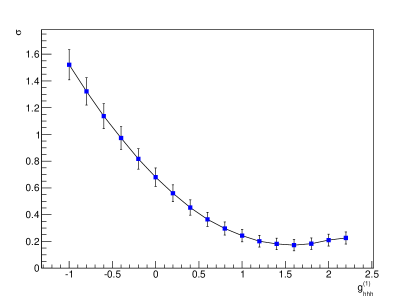
(a)

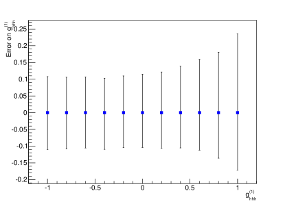
(b)

Figure 1: (a) Variation of cross section of the signal process $\sigma(pe^{-}\to\nu_{e}hhj,h\to b\bar{b})$ with respect to $g^{(1)}_{hhh}$ with error bar at each value of $g^{(1)}_{hhh}$, (b) local error through linear interpolation at each value of $g^{(1)}_{hhh}$.

4.2 Statistical analysis

Following the method given in Ref. [6], exclusion limits for $g^{(1)}_{hhh}$ are calculated. Fig. 1 shows significant behaviour of cross section variation with respect to $g^{(1)}_{hhh}$, which is expected, due to interference between resonant and non-resonant Higgs mediation in the charge-current signal process. The 95% upper limits of all effective couplings appear in the Lagrangian Eqs. (12), (13) and (14) due to cross section influence, are also calculated and shown in Fig. 2. The sensitivity of CP-even and odd $HWW$ effective couplings, $g^{(1)}_{hWW}$ and $\tilde{g}_{hWW}$, are of the same order as $g^{(1)}_{hhh}$ $\sim 10^{0}$. However, for $g^{(2)}_{hhh}\sim 10^{-3}-10^{-4}$ and $g^{(2)}_{hWW}$, $g^{(1,2)}_{hhWW}$, $\tilde{g}_{hhWW}$, these are of the order $\sim 10^{-2}$.

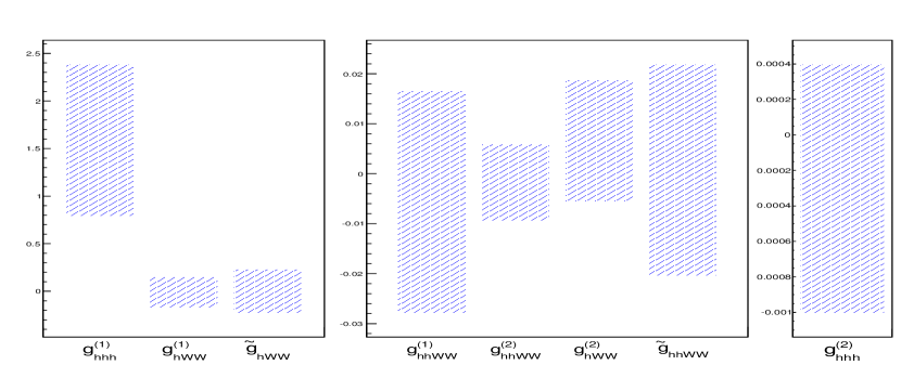
(a)

Figure 2: The limits on the coupling strength, derived at 0.4 ${\rm ab}^{-1}$. The $g^{(2)}_{hhh}$ has only the upper limit because the cross section dependence is monotonic in this region.

5 Conclusion

We briefly reviewed the physics potential of future $e^{-}p$ colliders, speculated to build on top of the LHC, through the top quark and Higgs boson physics. And we infer that the LHeC and the FCC-he is a viable option to study top and Higgs physics, and for the measurement of related couplings to high accuracy.

References

References

• [1] S.Β Dutta, A.Β Goyal, M.Β Kumar and B.Β Mellado, arXiv:1307.1688 [hep-ph].
• [2] T.Β Han and B.Β Mellado, Phys.Β Rev.Β D 82, 016009 (2010) [arXiv:0909.2460 [hep-ph]].
• [3] S.Β S.Β Biswal, R.Β M.Β Godbole, B.Β Mellado and S.Β Raychaudhuri, Phys.Β Rev.Β Lett.Β  109, 261801 (2012) [arXiv:1203.6285 [hep-ph]].
• [4] In preparation: M.Β Kumar, X.Β Ruan, A.Β Cornell, R.Β Islam, M.Β Klein, U.Β Klein, B.Β Mellado
• [5] V.Β M.Β Budnev, I.Β F.Β Ginzburg, G.Β V.Β Meledin and V.Β G.Β Serbo, Phys.Β Rept.Β  15 (1975) 181.
• [6] G.Β Cowan, K.Β Cranmer, E.Β Gross and O.Β Vitells, Eur.Β Phys.Β J.Β C 71 (2011) 1554 [Erratum-ibid.Β C 73 (2013) 2501] [arXiv:1007.1727 [physics.data-an]].