Abstract

We generalise the Jacob-Wick helicity formalism, which applies to sequential decays, to effective field theories of rare decays of the type $B\to K_{J_{K}}(\to K\pi)\bar{\ell}_{1}\ell_{2}$. This is achieved by reinterpreting local interaction vertices $\bar{b}\Gamma^{\prime}_{\mu_{1}..\mu_{n}}s\bar{\ell}\Gamma^{\mu_{1}..\mu_{n}}\ell$ as a coherent sum of $1\to 2$ processes mediated by particles whose spin ranges between zero and $n$. We illustrate the framework by deriving the full angular distributions for $\bar{B}\to\bar{K}\ell_{1}\bar{\ell}_{2}$ and $\bar{B}\to\bar{K}^{*}(\to\bar{K}\pi)\ell_{1}\bar{\ell}_{2}$ for the complete dimension-six effective Hamiltonian for non-equal lepton masses. Amplitudes and decay rates are expressed in terms of Wigner rotation matrices, leading naturally to the method of moments in various forms. We discuss how higher-spin operators and QED corrections alter the standard angular distribution used throughout the literature, potentially leading to differences between the method of moments and the likelihood fits. We propose to diagnose these effects by assessing higher angular moments. These could be relevant in investigating the nature of the current LHCb anomalies in $R_{K}={\cal B}(B\to K\mu^{+}\mu^{-})/{\cal B}(B\to Ke^{+}e^{-})$ as well as angular observables in $B\to K^{*}\mu^{+}\mu^{-}$.

1 Introduction

Helicity amplitudes (HAs), as defined by Jacob and Wick [1], describe $A\to BC$ ($1\to 2$) transitions and have definite transformation properties under rotation. The key idea is that the angular and helicity information are equivalent to each other. Angular decay distributions follow (e.g. [2, 3, 4]) from evaluating the HAs with $B$ and $C$ in the forward direction, with the angular information encoded in Wigner $D$ matrix functions, reminiscent of the Wigner-Eckart theorem.

The intent of this paper is to generalise this method to decays of the type $A\to(B_{1}B_{2})C$ which are schematically described by local interactions of the form

$$H^{\rm eff}\sim(AC)_{\mu_{1}\dots\mu_{n}}(B_{1}B_{2})^{\mu_{1}\dots\mu_{n}}\;.$$ (1)

We do so by rewriting the $1\to 3$ decay as a sequence of $1\to 2$ processes, by inserting multiple complete sets of polarisation states between the Lorentz contractions of $AC$ and $B_{1}B_{2}$ above. This leads to a reinterpretation of the decay in terms of a sum over intermediate particles of spin $J$, where $J$ can range from $0$ up to $n$ depending on the specific structure of the operators. Symbolically we may write

$${\cal A}(A\to(B_{1}B_{2})C)=\sum_{J\geq 0}^{n}{\cal A}(A\to B_{J}(\to B_{1}B_{2})C)\;,$$ (2)

with ${\cal A}$ denoting the amplitude. We refer to this case as the $B$-particle factorisation approximation. At the formal level, the main work is the decomposition of the Lorentz tensors into irreducible objects under the spatial rotation group (reminiscent of the $3+1$ decomposition of cosmological perturbation theory for example).

Important examples of such decays are given by the rare radiative decays $B\to K\ell^{+}\ell^{-}$ and $B\to K^{*}(\to K\pi)\ell^{+}\ell^{-}$. Besides evaluating non-perturbative matrix elements to these decays (e.g. [5, 6, 7, 8, 9, 10, 11, 12, 13, 14, 15, 16, 17]), it has become clear that it is beneficial to consider general properties of the amplitudes entering the angular distributions (e.g. [18, 19, 20, 21]). Our work can be seen to be part of the latter category.

We evaluate the $\bar{B}\to\bar{K}^{(*)}\ell^{+}\ell^{-}$ angular decay distributions within the generalised helicity framework developed in this paper, providing an alternative method to traditional techniques using Dirac trace technology [22, 23]. An important consequence of the manner in which we derive the distribution is that it lends itself to the methods of moments (MoM), which use the decomposition of the distribution into orthogonal functions to obtain observables independently of each other. This is a complementary method to the likelihood fit to extract the dynamical information from the decay, and was recently studied from an experimental viewpoint in [24]. We discuss the impact of including higher partial waves in both the $(K\pi)$- and especially the dilepton-system. The latter give rise to corrections, in the form of higher moments, to the standard form of the angular distribution used in the literature. The sources of higher dilepton partial waves are higher spin operators and electroweak corrections, both of which we discuss qualitatively. The two sources can be distinguished by their different behaviour in higher partial moments. We encourage experimental investigation of higher moments from various viewpoints. In particular, we discuss how higher moments can be used to diagnose the size of QED effects in $B\to K\ell^{+}\ell^{-}$ (with $\ell=e,\mu$) and test leakage of $J/\Psi$-contributions into the lower dilepton-spectrum. Both are of importance in view of $R_{K}$ as well as the angular anomalies in the low dilepton-spectrum, which have recently been reported by the LHCb collaboration in [25] and [26, 27] respectively.

The paper is organised as follows. In section 2 the methodology is introduced ending with a formal expression for the fourfold decay distribution in terms of rotation matrices and HAs. Specific angular distributions for $\bar{B}\to\bar{K}^{(*)}\ell_{1}\bar{\ell}_{2}$, with detailed results in appendices C (and a Mathematica notebook in the arXiv version) and D, are given in section 3. The method of total and partial moments is presented in section 4. Section 5 contains the discussion of including higher partial waves: a qualitative assessment of higher spin operators and QED corrections is presented in subsections 5.2 and 5.3 respectively. The relevance of testing for higher moments is emphasised in subsection 5.4. The paper ends with conclusions in section 6. Additional material, such as the leptonic HAs and a few brief remarks on $\Lambda_{b}\to\Lambda\left(\to(p,n)\pi\right)\ell_{1}\bar{\ell}_{2}$, is presented in appendices A.3 and E respectively. In appendix B we provide the kinematic conventions for computation of the angular distribution by the sole use of Dirac trace technology.

2 Generalised Helicity Formalism for Effective Theories

We first review the standard helicity formalism in section 2.1, and qualitatively apply it to sequential $1\to 2$ decays in section 2.1.1, specialising to the spin configuration relevant for our decays at the end. In section 2.2 the formalism is extended to include decays like $B\to K_{J_{K}}(\to K\pi)\bar{\ell}_{1}\ell_{2}$ described by effective field theories for $b\to s\bar{\ell}_{1}\ell_{2}$ transitions. The framework can be straightforwardly applied to the entire zoo of semi-leptonic and rare flavour decays such as $B_{s}\to K^{*}\ell\nu$, $B\to D^{(*)}\ell\nu$, $D\to(\pi,\rho)\mu\mu$, $D\to(\pi,\rho)\mu\nu$, $K\to\pi\mu\mu$ etc., and can also be extended to include initial particles with non-zero spin.

2.1 The basic idea of the Helicity Formalism and its Extension

The discussion in this section is standard and we refer the reader to [2, 3, 4] for more extensive reviews, as well as the pioneering paper of Jacob and Wick [1]. In a $1\to 2$ (say $A\to B_{1}B_{2}$) decay a particle of spin $J_{A}$ and helicity $M_{A}$ decays into two particles of momentum $\vec{p}_{1}$ and $\vec{p}_{2}$ with helicities $\lambda_{1}$ and $\lambda_{2}$ respectively. In the centre-of-mass frame ($\vec{p}_{1}=-\vec{p}_{2}$) the system can be characterised by the two helicities and the direction (i.e. the solid angles $\theta$ and $\phi$). By inserting a complete set of two-particle angular momentum states the corresponding matrix element can be written

$${\cal A}(A\to B_{1}B_{2}) = \langle\theta,\phi,\lambda_{1},\lambda_{2}|J_{A},M_{A}\rangle=\sum_{j,m}\langle\theta,\phi,\lambda_{1},\lambda_{2}|j,m,\lambda_{1},\lambda_{2}\rangle\langle j,m,\lambda_{1},\lambda_{2}|J_{A},M_{A}\rangle$$ (3)

$$= \underbrace{\langle\theta,\phi,\lambda_{1},\lambda_{2}|J_{A},M_{A},\lambda_{1},\lambda_{2}\rangle}_{\sqrt{\frac{2J_{A}+1}{4\pi}}D^{J_{A}}_{M_{A},\lambda_{1}-\lambda_{2}}\left(\phi,\theta,-\phi\right)}\underbrace{\langle J_{A},M_{A},\lambda_{1},\lambda_{2}|J_{A},M_{A}\rangle}_{\!\!\!{\phantom{\sqrt{\frac{1}{1}}}}{\cal A}^{J_{A}}_{M_{A},\lambda_{1},\lambda_{2}}}$$

as a product of Wigner $D$-functions and a HA ${\cal A}^{J_{A}}_{M_{A},\lambda_{1},\lambda_{2}}$. The Wigner matrix is a $(2J_{A}+1)$-dimensional $SO(3)$ representation in the helicity basis. The essence is that the distribution of the amplitude over the angles is then governed by the rotation matrix as a function of the helicities. In practice one only needs to compute the HA.

The process $B\to J/\Psi(\to\ell^{+}\ell^{-})K^{*}(\to K\pi)$ constitutes a well-known example of a sequential $1\to 2$ decay where the formalism can be applied [29]. The idea of this paper is to extend this formalism to the case where the $\bar{\ell}_{1}\ell_{2}$-pair emerges from a local interaction vertex $O_{ij}\sim\bar{s}\Gamma_{i}b\bar{\ell}\Gamma_{j}\ell$ with effective Hamiltonian $H^{\rm eff}\sim\sum_{ij}C_{ij}O_{ij}$. This is achieved by reinterpreting the local interaction vertex as originating from a sum of particles whose spin depends on the number of Lorentz contractions between the $\Gamma_{i,j}$ structures. Elements of this program have appeared in the literature, e.g. [30] for $B\to K_{J}\ell^{+}\ell^{-}$, but we are unaware of a systematic presentation that allows the incorporation of a generic effective Hamiltonian as well as other decay types.

2.1.1 Helicity formalism for $B_{J_{B}}\to K_{J_{K}}(\to K_{1}K_{2})\gamma_{J_{\gamma}}(\to\bar{\ell}_{1}\ell_{2})$

Let us consider the following sequential decay

$$B_{J_{B}}\to K_{J_{K}}(\to K_{1}K_{2})\gamma_{J_{\gamma}}^{\vphantom{+}}(\to\bar{\ell}_{1}\ell_{2})$$ (4)

where $J_{B}$, $J_{\gamma}$ and $J_{K}$ denote the spin of the particles $B$, $\gamma_{J}^{\vphantom{+}}$ and $K_{J}$. The notation is close to the main application of this paper but we emphasise that at this point the methodology is completely general. Assuming the decay to be a series of sequential $1\to 2$ decays the amplitude can be written in terms of a product of $1\to 2$ HAs times the corresponding Wigner functions

$$\begin{split}&{\cal A}(\Omega_{B},\Omega_{\ell},\Omega_{K}|\lambda_{B},\lambda_{K_{1}},\lambda_{K_{2}},\lambda_{1},\lambda_{2})\sim\\ &\quad\sum_{\lambda_{\gamma}\lambda_{K}}\bar{D}^{J_{B}}_{\lambda_{B},\lambda_{\gamma}-\lambda_{K}}\left(\Omega_{B}\right){\cal H}_{\lambda_{\gamma}\lambda_{K}}\bar{D}^{J_{K}}_{\lambda_{K},\lambda_{K_{2}}-\lambda_{K_{1}}}\left(\Omega_{K}\right){\cal K}_{\lambda_{K_{1}},\lambda_{K_{2}}}\bar{D}^{J_{\gamma}}_{\lambda_{\gamma},\lambda_{\ell}}\left(\Omega_{\ell}\right){\cal L}_{\lambda_{\ell_{1}}\lambda_{\ell_{2}}}\;,\end{split}$$ (5)

where the $\lambda_{i}$ are helicity indices, and

$$\lambda_{\ell}\equiv\lambda_{1}-\lambda_{2}\;,$$ (6)

is a shorthand that we use frequently throughout the paper. The HAs ${\cal H}$, ${\cal K}$ and ${\cal L}$ correspond to the transitions $B_{J_{B}}\to K_{J_{K}}\gamma_{J_{\gamma}}$, $K_{J_{K}}\to K_{1}K_{2}$ and $\gamma_{J_{\gamma}}\to\bar{\ell}_{1}\ell_{2}$ respectively. The helicities of the internal particles $\gamma_{J}$ and $K_{J}$ have to be coherently summed over. The Wigner $D$-functions

$$D^{j}_{m^{\prime},m}\left(\Omega=(\alpha,\beta,\gamma)\right)=\langle jm^{\prime}|e^{-i\alpha J_{z}}e^{-i\beta J_{y}}e^{-i\gamma J_{z}}|jm\rangle$$ (7)

are irreducible $SO(3)$-representations of dimension $2j+1$. The $J_{i}$ are the generators of angular momentum, and the states $|j,m\rangle$ carry angular momentum $j$ and helicity $m$ and are orthonormalised $\langle j,m|j^{\prime},m^{\prime}\rangle=\delta_{jj^{\prime}}\delta_{mm^{\prime}}$. To avoid proliferation of indices we denote complex conjugation by a bar instead of the more standard asterisk.

Adaptation to $J_{B}=0$ and $K_{1}=K$ and $K_{2}=\pi$

In order to ease the notation slightly we move straight to the case $\bar{B}\to\bar{K}_{J}(\to K\pi)\gamma_{J_{\gamma}}(\to\ell_{1}\bar{\ell}_{2})$. The relation $D_{\lambda_{B}=0,\lambda_{\gamma}-\lambda_{K}}^{J_{B}=0}(\Omega)=\delta_{0,\lambda_{\gamma}-\lambda_{K}}$ implies equality of helicities

$$\lambda\equiv\lambda_{\gamma}=\lambda_{K}\;.$$ (8)

One may therefore reduce ${\cal H}_{\lambda_{\gamma}\lambda_{K}}\to H_{\lambda}$, which is the quantity known as the HA in the $\bar{B}\to\bar{K}^{*}\ell^{+}\ell^{-}$-literature and carries the non-trivial dynamic information. The HA ${\cal K}_{\lambda_{K_{1}},\lambda_{K_{2}}}$ reduces to a scalar constant (denoted by $g_{K_{J}K\pi}$) since $K_{1}\to K$, $K_{2}\to\pi$ are both scalar particles. The third HA ${\cal L}_{\lambda_{1}\lambda_{2}}$ depends on the interaction vertex of the leptons, but is trivial to calculate once the interaction is known. We may rewrite the amplitude (5) as

$${\cal A}(\bar{B}\to\bar{K}_{J_{K}}(\to K\pi)\gamma_{J_{\gamma}}(\to\ell_{1}\bar{\ell}_{2}))\sim\sum_{\lambda=-J_{K}}^{J_{K}}D^{J_{K}}_{\lambda,0}\left(\Omega_{K}\right)D^{J_{\gamma}}_{\lambda,\lambda_{\ell}}\left(\Omega_{\ell}\right){\cal A}^{J_{\gamma}}_{\lambda,\lambda_{1},\lambda_{2}}\;,$$ (9)

where the angles, depicted in figure 1, are $\Omega_{K}=(0,\theta_{K},0)$ and $\Omega_{\ell}=(\phi_{\ell},\theta_{\ell},-\phi_{\ell})$. Note, the passage from $\bar{D}$ to $D$-functions from (5) to (9) is related to passing from $B$ to $\bar{B}$.

In the lepton-pair factorisation approximation, defined more explicitly in the following section, the amplitude ${\cal A}^{J_{\gamma}}_{\lambda,\lambda_{1},\lambda_{2}}\sim H_{\lambda}{\cal L}_{\lambda_{1}\lambda_{2}}|_{J_{\gamma}}$ is the product of the hadronic and leptonic matrix elements. The angle $\phi_{\ell}$ is the helicity angle and is usually called simply $\phi$. Before commenting on different conventions of the angles we quote the fourfold differential decay

$$\frac{d^{4}\Gamma}{dq^{2}d\cos\theta_{\ell}d\cos\theta_{K}d\phi}\sim\sum_{\lambda_{1}\lambda_{2}}|{\cal A}|^{2}\sim$$ (10)

$$\sum_{\lambda_{1},\lambda_{2}=-1/2}^{1/2}\sum_{\lambda,\lambda^{\prime}=-J_{\gamma}}^{J_{\gamma}}{{\cal A}}^{J_{\gamma}}_{\lambda,\lambda_{1},\lambda_{2}}\bar{{\cal A}}^{J_{\gamma}}_{\lambda^{\prime},\lambda_{1},\lambda_{2}}D^{J_{K_{J}}}_{\lambda,0}\left(\Omega_{K}\right)\bar{D}^{J_{K_{J}}}_{\lambda^{\prime},0}\left(\Omega_{K}\right)D^{J_{\gamma}}_{\lambda,\lambda_{\ell}}\left(\Omega_{\ell}\right)\bar{D}^{J_{\gamma}}_{\lambda^{\prime},\lambda_{\ell}}\left(\Omega_{\ell}\right)\;,$$ (11)

in terms of amplitudes and Wigner $D$-functions. For the angles we use the $\bar{B}\to\bar{K}^{*}\ell\ell$ decay as a reference and use the same conventions as the LHCb collaboration [31] (appendix A), which differ from those used by the theory community. More precise statements, including a conversion diagram, can be found in appendix C.2.

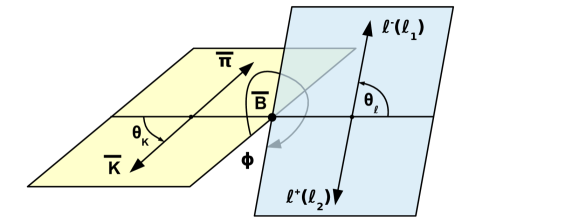
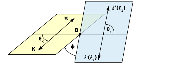
Figure 1: Decay geometries for $\bar{B}\to\bar{K}^{*}\ell_{1}\bar{\ell}_{2}$ (above) and $B\to K^{*}\bar{\ell}_{1}\ell_{2}$ (below). In both cases $\ell_{1}=\ell^{-}$, $\ell_{2}=\ell^{-}$ denote the negatively charged lepton. The conventions are the same as used by the LHCb collaboration in [31] (cf. appendix A therein). Comparison to the convention used by the theory community can be found in appendix C.2. The pictures are slightly misleading in that the angles $\theta_{\ell,K}$ are drawn in the restframe of the lepton-pair and the $K^{*}$-meson. For decays which are not self-tagging, such as $B_{s},\bar{B}_{s}\to\phi(\to K^{+}K^{-})\mu^{+}\mu^{-}$ at the LHCb, the angles $(\theta_{\ell},\theta_{K},\phi)\to(\pi-\theta_{\ell},\pi-\theta_{K},2\pi-\phi),$ and one can only measure the sum of both decay rates (second equation(C.2)).

2.2 Effective Theories rewritten as a coherent Sum of Sequential Decays

In this section we give the formal steps to derive the expression of the angular distributions. The reader interested in the final result can directly proceed to section 3.

The amplitude (9) is of a completely general form for the decay where $\gamma_{J_{\gamma}}$ is an actual particle of spin $J_{\gamma}$. In $\bar{B}\to\bar{K}^{*}(\to\bar{K}\pi)\ell_{1}\bar{\ell}_{2}$ a part of the amplitude is in this form where the photon corresponds to the intermediate state ($\gamma_{1}=\gamma$). In general there are effective vertices, so-called contact terms, where the intermediate particles are not present. In the interest of clarity we quote the effective Hamiltonian for $b\to s\ell\bar{\ell}$:

$$H^{\rm eff}=c_{H}\hat{H}^{\rm eff}\;,\quad c_{H}\equiv-\frac{4G_{F}}{\sqrt{2}}\frac{\alpha}{4\pi}V_{\rm ts}^{*}V_{\rm tb}\;,\quad\hat{H}^{\rm eff}=\!\!\!\!\!\!\!\!\!\sum_{i=V,A,S,P,\cal T}(C_{i}O_{i}+C^{\prime}_{i}O^{\prime}_{i})\;.\quad$$ (12)

Above $G_{F}$ is Fermi’s constant, $\alpha$ the fine structure constant, $V_{\rm tD}$ are Cabibbo-Kobayashi-Maskawa (CKM) elements and the operators are

$$O_{S(P)}=\bar{s}_{L}b\;\bar{\ell}(\gamma_{5})\ell\;,\quad O_{V(A)}=\bar{s}_{L}\gamma^{\mu}b\;\bar{\ell}\gamma_{\mu}(\gamma_{5})\ell\;,\quad O_{\cal T}=\bar{s}_{L}\sigma^{\mu\nu}b\;\bar{\ell}\sigma_{\mu\nu}\ell\;,$$ (13)

where $O^{\prime}=O|_{s_{L}\to s_{R}}$, the labels refer to the lepton interaction vertex, $q_{L,R}\equiv 1/2(1\mp\gamma_{5})q$, $\bar{\ell},\ell\to\bar{\ell}_{1},\ell_{2}$ for different lepton flavours and a few additional relevant remarks deferred to appendix A.2. In passing we add that the notation $O_{9(10)}=O_{V(A)}$ is more common throughout the literature. In the case where electroweak corrections are neglected at the matrix element level one may factorise the hadronic from the leptonic part. We refer to this as the lepton-pair factorisation approximation (LFA) ($B$-particle factorisation approximation in the introduction). Schematically (12) is written as a product of a hadronic part $H$ and a leptonic part ${\mathcal{L}}$ with a certain number of Lorentz contractions between them:

$$H^{\rm eff}\sim\sum_{a=1}^{N_{0}}H^{a}{\mathcal{L}}_{a}+\sum_{b=1}^{N_{1}}H^{b}_{\mu}{\mathcal{L}}_{b}^{\mu}+\sum_{c=1}^{N_{2}}H^{c}_{\mu_{1}\mu_{2}}{\mathcal{L}}_{c}^{\mu_{1}\mu_{2}}\;.$$ (14)

The sum over $a$, $b$ and $c$ extends over operators with $0$, $1$ and $2$ Lorentz contractions between quark and lepton operators. In the example of $C_{V}O_{V}=H_{\mu}\cal L^{\mu}$ we would have $H_{\mu}=C_{V}\bar{s}_{L}\gamma_{\mu}b$ and $\cal L^{\mu}=\bar{\ell}\gamma^{\mu}\ell$. On a formal level we might think of $O_{V}(O_{9})$ as originating from integrating out a vector and a scalar particle, in the sense that the Lorentz contraction over index $\mu$ can be written as the sum of products of a spin-one and a timelike spin-$0$ polarisation vector. This is expressed by the well-known completeness relation (e.g. [23, 30, 18])

$$g^{\mu\nu}=\sum_{\lambda,\lambda^{\prime}\in\{t,\pm,0\}}\omega^{\mu}(\lambda)\bar{\omega}^{\nu}(\lambda^{\prime})G_{\lambda\lambda^{\prime}}\;,\quad G_{\lambda\lambda^{\prime}}=\text{diag}(1,-1,-1,-1)\;,$$ (15)

where the first entry in $G_{\lambda\lambda^{\prime}}$ refers to $\lambda=\lambda^{\prime}=t$ and an explicit parametrisation is given by

$$\omega^{\mu}(\pm)=(0,\pm 1,i,0)/\sqrt{2}\;,\quad\omega^{\mu}(0)=(q_{z},0,0,q_{0})/\sqrt{q^{2}}\;,\quad\omega^{\mu}(t)=(q_{0},0,0,q_{z})/\sqrt{q^{2}}\;,$$ (16)

which is consistent with the parameterisation $q^{\mu}=(q_{0},0,0,q_{z})$. The polarisation vectors $\omega(\pm,0)$ are compatible with the Jacob-Wick phase convention [1] (cf. appendix B and the corresponding footnote for further remarks). Let us pause a moment and emphasise that intermediate results do depend on the convention, which enters the definition of the HAs, and this dependence has to be taken into account when comparing to HAs appearing in the literature. We choose the convention in [18], since it is compatible with the Condon-Shortly convention that is standard for Clebsch-Gordon coefficients and Wigner matrices (e.g. [32]).

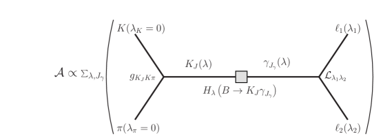
Figure 2: A diagrammatic interpretation of the process, equation (22), used to set up the formalism. The decay to two leptons is treated as being mediated by an effective particle $\gamma_{J_{\gamma}}$ of spin $J_{\gamma}$. The factor $g_{K_{J}K\pi}$ has no dependence on helicities and depends only on the dynamics of the $K^{*}$ decay.

We may think of $\omega$ as being associated with the Lorentz group $SO(3,1)$. In the rest frame $q_{z}=0$ the timelike polarisation tensor transforms as a scalar under the restriction of $SO(3,1)$ to spatial rotations $SO(3)$. For an effective operator with $n$ Lorentz indices the relation (15) can be inserted $n$ times to obtain a HA with $n$ helicity indices. More precisely, the direct product of $SO(3,1)$ polarisation tensors decomposes into irreducible representations of $SO(3)$ polarisation tensors $\epsilon^{j,\lambda}_{\mu_{1}\dots\mu_{n}}$ of spin $j=0,\dots,n$ and helicities $\lambda=-j,\dots,j$. Using the expressions in Eqs. A.8 and A.9 the analogue of ${\cal A}^{J_{\gamma}}_{\lambda,\lambda_{1},\lambda_{2}}$ in (9) on each spin component can be written as

$${\cal A}^{J_{\gamma}}_{\lambda,\lambda_{1},\lambda_{2}}=\left\{\begin{array}[]{llll}\;\langle H_{a}\rangle\langle{\mathcal{L}}_{a}\rangle\;\;+&\langle H_{b}^{\mu}\rangle\langle{\mathcal{L}}_{b}^{\alpha}\rangle\epsilon^{0,0}_{\mu}\bar{\epsilon}_{\alpha}^{0,0}&+\;\;\langle H_{c}^{\mu\nu}\rangle\langle{\mathcal{L}}_{c}^{\alpha\beta}\rangle\epsilon^{0,0}_{\mu\nu}\cdot\bar{\epsilon}^{0,0}_{\alpha\beta}&\quad J_{\gamma}=0\\ &\langle H_{b}^{\mu}\rangle\langle{\mathcal{L}}_{b}^{\alpha}\rangle\epsilon^{1,\lambda}_{\mu}\bar{\epsilon}^{1,\lambda_{\ell}}_{\alpha}&+\;\;\langle H_{c}^{\mu\nu}\rangle\langle{\mathcal{L}}_{c}^{\alpha\beta}\rangle\epsilon^{1,\lambda}_{\mu\nu}\cdot\bar{\epsilon}^{1,\lambda_{\ell}}_{\alpha\beta}&\quad J_{\gamma}=1\\ &&\phantom{+}\;\;\langle H_{c}^{\mu\nu}\rangle\langle{\mathcal{L}}_{c}^{\alpha\beta}\rangle\epsilon^{2,\lambda}_{\mu\nu}\cdot\bar{\epsilon}^{2,\lambda_{\ell}}_{\alpha\beta}&\quad J_{\gamma}=2\end{array}\right.$$ (20)

where summation over Lorentz indices and the number of operators in (14) are both implied, the scalar product “$\cdot$” is detailed in (A.8) and

$$\langle H_{a}^{\mu_{1}\dots\mu_{n}}\rangle\equiv\langle\bar{K}_{J}(\lambda)|H_{a}^{\mu_{1}\dots\mu_{n}}|\bar{B}\rangle\;,\quad\langle{\mathcal{L}}_{a}^{\mu_{1}\dots\mu_{n}}\rangle\equiv\langle\ell_{1}(\lambda_{1})\bar{\ell}_{2}(\lambda_{2})|{\mathcal{L}}_{a}^{\mu_{1}\dots\mu_{n}}|0\rangle\;,$$ (21)

are the leptonic and hadronic matrix elements. The helicities in (20) are the helicities of the outgoing particles of the HAs, with $\lambda$ for $K_{J}(\lambda)$ in $H^{B\to K_{J_{K}}}$ and $\lambda_{\ell}=\lambda_{1}-\lambda_{2}$ for $\ell_{1}(\lambda_{1})\bar{\ell}_{2}(\lambda_{2})$ in $\mathcal{L}^{\gamma_{J_{\gamma}}\to\ell_{1}\bar{\ell}_{2}}$. This is the main idea of the formalism: the angular dependence from the ingoing to outgoing particle is governed by the Wigner $D$-function, e.g. $\bar{\epsilon}^{J_{\ell,\lambda}}=\bar{D}^{J_{\gamma}}_{\lambda,\lambda_{\ell}}\left(\Omega_{\ell}\right)\bar{\epsilon}^{J_{\ell,\lambda_{\ell}}}$ for $\mathcal{L}^{\gamma_{J_{\gamma}}(\lambda)\to\ell_{1}(\lambda_{1})\bar{\ell}_{2}(\lambda_{2})}$, which is inherent in (3). The generalised HA then becomes essentially a sum over all spin components $J_{\gamma}$ necessary to saturate the Lorentz indices in the effective Hamiltonian,

$${\cal A}(\bar{B}\to\bar{K}_{J_{K}}(\to K\pi)\ell_{1}\bar{\ell}_{2})=\frac{\sqrt{2J_{K}+1}}{4\pi}\;\;\sum_{J_{\gamma}=0}^{n}\sum_{\lambda=-{\rm min}(J_{\gamma},J_{K})}^{{\rm min}(J_{\gamma},J_{K})}D^{J_{K}}_{\lambda,0}\left(\Omega_{K}\right)D^{J_{\gamma}}_{\lambda,\lambda_{\ell}}\left(\Omega_{\ell}\right){\cal A}^{J_{\gamma}}_{\lambda,\lambda_{1},\lambda_{2}}\;,$$ (22)

where the overall factor follows from (3). A schematic representation of equation (22) is given in figure 2. The differential decay distribution (10) is replaced by a similar expression

$$\frac{d^{4}\Gamma}{dq^{2}d\cos\theta_{\ell}d\cos\theta_{K}d\phi}\sim\sum_{\lambda_{1}\lambda_{2}}|{\cal A}|^{2}=\frac{2J_{K}+1}{4\pi}\sum_{\lambda_{1}\lambda_{2}}\sum_{J_{\gamma}\lambda}\sum_{J_{\gamma}^{\prime}\lambda^{\prime}}\times$$

$${\cal A}^{J_{\gamma}}_{\lambda,\lambda_{1},\lambda_{2}}\bar{{\cal A}}^{J_{\gamma}^{\prime}}_{\lambda^{\prime},\lambda_{1},\lambda_{2}}D^{J_{K}}_{\lambda,0}\left(\Omega_{K}\right)\bar{D}^{J_{K}}_{\lambda^{\prime},0}\left(\Omega_{K}\right)D^{J_{\gamma}}_{\lambda,\lambda_{\ell}}\left(\Omega_{\ell}\right)\bar{D}^{J_{\gamma}}_{\lambda^{\prime},\lambda_{\ell}}\left(\Omega_{\ell}\right)\;,$$ (23)

with additional coherent sums over the spins $J_{\gamma}$

$$\sum_{\lambda_{1}\lambda_{2}}=\sum_{\lambda_{1},\lambda_{2}=-1/2}^{1/2}\;,\quad\sum_{J_{\gamma}\lambda}=\sum_{J_{\gamma}=0}^{2}\sum_{\lambda=-\min(J_{\gamma},J_{K_{J}})}^{\min(J_{\gamma},J_{K_{J}})}$$ (24)

and likewise for the sum over $J_{\gamma}^{\prime},\lambda^{\prime}$.

3 Angular distribution and Wigner $D$-functions

We now apply the method introduced in the previous section to decays governed by the $b\to s\ell_{1}\bar{\ell}_{2}$ effective Hamiltonian (12). First we consider the decay $\bar{B}\to\bar{K}^{*}\left(\to\bar{K}\pi\right)\ell_{1}\bar{\ell}_{2}$, and then in section 3.3 we present similar results for $\bar{B}\to\bar{K}\ell_{1}\bar{\ell}_{2}$. The related decay $\Lambda_{b}\to\Lambda\left(\to N\pi\right)\ell_{1}\bar{\ell}_{2}$, where $N=(p,n)$, can also be treated within this formalism, and will be briefly considered in appendix E.

3.1 $\bar{B}\to\bar{K}^{*}\left(\to\bar{K}\pi\right)\ell_{1}\bar{\ell}_{2}$

The use of the effective Hamiltonian (12) in the LFA restricts the partial waves to $J_{\gamma}=0,1$ terms in equation (20). The discussion of higher partial waves ( $J_{\gamma}\geq 2$) is deferred to section 5. The matrix element for (12) is then given by the sum of an $S_{\ell}$- and $P_{\ell}$-wave amplitude (with the subscript $\ell$ referring to the partial wave in the angle $\theta_{\ell}$):

$$\hat{\mathcal{M}}_{\lambda_{1},\lambda_{2}} =\langle\bar{K}^{*}(\to\bar{K}\pi)\ell_{1}(\lambda_{1})\bar{\ell}_{2}(\lambda_{2})|\hat{H}^{\rm eff}|\bar{B}\rangle$$

$$=\frac{\sqrt{3}}{4\pi}\left[{\cal A}^{0}_{0,\lambda_{1},\lambda_{2}}D^{1}_{0,0}\left(\Omega_{K}\right)\delta_{\lambda_{1}\lambda_{2}}+\sum_{\lambda=\pm,0}{\cal A}^{1}_{\lambda,\lambda_{1},\lambda_{2}}D^{1}_{\lambda,0}\left(\Omega_{K}\right)D^{1}_{\lambda,\lambda_{\ell}}\left(\Omega_{\ell}\right)\right]\;,$$ (25)

where the hat denotes the effective Hamiltonian without the $c_{H}$ prefactor (12). There is no $D$-wave since the two-indices in the tensor operator (12) are antisymmetric and therefore in a spin $1$ representation (cf. discussion in section 5.2 on higher spin operators). The $K^{*}$ has spin $1$ and is therefore always in a $P_{K}$-wave in the $\theta_{K}$-angle, with analogous meaning for the $K$ subscript as before. Above we have used $D^{0}_{0,\lambda_{\ell}}\left(\Omega\right)=\delta_{0\lambda_{\ell}}$ to impose $\delta_{\lambda_{1}\lambda_{2}}$ on the scalar part of the matrix element. The principal objects to be calculated are the amplitudes ${\cal A}^{J_{\gamma}}_{\lambda,\lambda_{1},\lambda_{2}}$. For $H^{\rm eff}$ (12) the $S_{\ell}$- and $P_{\ell}$-wave amplitudes (that is to say ${\cal A}^{0}$ and ${\cal A}^{1}$ respectively) are written as

$${\cal A}^{0}_{0,\lambda_{1},\lambda_{2}} =H^{S}\mathcal{L}^{S}_{\lambda_{1},\lambda_{2}}+H^{P}\mathcal{L}^{P}_{\lambda_{1},\lambda_{2}}\;,$$

$${\cal A}^{1}_{\lambda,\lambda_{1},\lambda_{2}} =-H_{\lambda}^{V}\mathcal{L}^{V}_{\lambda_{1},\lambda_{2}}-H_{\lambda}^{A}\mathcal{L}^{A}_{\lambda_{1},\lambda_{2}}+H^{T}_{\lambda}\mathcal{L}^{T}_{\lambda_{1},\lambda_{2}}-2H^{T_{t}}_{\lambda}\mathcal{L}^{T_{t}}_{\lambda_{1},\lambda_{2}}\;,$$ (26)

with the relative signs and factor of 2 emerging from the (double) completeness relation (A.3), and the leptonic and the hadronic HAs are

$$H^{X}_{\lambda}=\langle\bar{K}^{*}(\lambda)|\bar{s}\overline{\Gamma}^{X}b|\bar{B}\rangle\;,\quad{\mathcal{L}}^{X}_{\lambda_{1}\lambda_{2}}\equiv\langle\ell_{1}(\lambda_{1})\bar{\ell}_{2}(\lambda_{2})|\bar{\ell}\Gamma^{X}\ell|0\rangle\;,$$ (27)

the expressions in (21) contracted with the corresponding polarisation vectors. Explicit results, as well as a more precise prescription concerning $\Gamma^{X}$, are given in Appendices A.3 and C.5 in Eqs. (A.13) and (C.14) respectively.

	$\Gamma^{S[P]}$	$\Gamma^{V[A]}$	$\Gamma^{T[T_{t}]}$
$\Gamma^{X}$	${\mathbf{1}}_{4}[\gamma_{5}]$	$\gamma^{\mu}[\gamma_{5}]\omega_{\mu}(\lambda_{X})$	$\sigma^{\mu\nu}\omega^{1,\lambda_{X}}_{\mu\nu}[\omega^{t,\lambda_{X}}_{\mu\nu}]$
$J_{\gamma}(X)$	0	1	1

Table 1: The definitions of the $\Gamma^{X}$ and their associated spin $J_{\gamma}(X)$. The contributions $J_{\gamma}(X)=0,1$ give rise to the $S_{\ell}$- and $P_{\ell}$-wave amplitudes respectively. The basic polarisation vector $\omega_{\mu}$ is given in (16) and the composed ones can be found in equation (A.1). The precise value of the helicity index $\lambda_{X}$ is specified when the leptonic and hadronic HAs are defined in Eqs. (A.13,C.14,D.4). Note that the additional structure $\Gamma^{T_{5}}=\sigma_{\mu\nu}\gamma_{5}$ can be absorbed into the other tensor structures due to the identity $\sigma^{\alpha\beta}\gamma_{5}=-\frac{i}{2}\epsilon^{\alpha\beta\mu\nu}\sigma_{\mu\nu}$ (with the $\epsilon_{0123}=+1$ convention for the Levi-Civita tensor). Timelike contributions $\gamma^{\mu}[\gamma_{5}]\omega_{\mu}(t)$ can be absorbed into $\Gamma^{S,P}$ respectively, as detailed in appendix C.5. Above $\sigma_{\mu\nu}=i/2[\gamma_{\mu},\gamma_{\nu}]$.

Squaring the matrix element in (3.1), summing over external helicities and averaging over final-state spins, one obtains an angular distribution

$$I_{K^{*}}\left(q^{2},\Omega_{K},\Omega_{\ell}\right) \equiv\frac{32\pi}{3}\frac{d^{4}\Gamma}{dq^{2}\;d\textrm{cos}\theta_{\ell}\;d\textrm{cos}\theta_{K}\;d\phi}=\frac{32\pi}{3}{\cal N}\sum_{\lambda_{1},\lambda_{2}}\left|\hat{\mathcal{M}}_{\lambda_{1},\lambda_{2}}\right|^{2}\;,\quad$$ (28)

with $I_{K^{*}}$ being a shorthand and $32\pi/3$ is a convenient normalisation factor. The factor ${\cal N}$,

$${\cal N}\equiv|c_{H}|^{2}\kappa_{\rm kin}\;,\quad\kappa_{\rm kin}\equiv\frac{\sqrt{\lambda_{B}}\sqrt{\lambda_{\gamma^{*}}}}{2^{6}\pi^{3}m_{B}^{3}q^{2}}\;,$$ (29)

is the product of the prefactor resulting from the effective Hamiltonian $c_{H}$ (12) and the kinematic phase space factor. The matrix element is defined in (3.1). Above $\lambda_{B}\equiv\lambda(m_{B}^{2},m_{K^{*}}^{2},q^{2})$ and $\lambda_{\gamma^{*}}\equiv\lambda(q^{2},m_{\ell_{1}}^{2},m_{\ell_{2}}^{2})$ where $\lambda(a,b,c)$ is the Källén-function defined in (B.1) and related to the absolute value of the three-momentum of the $K^{*}$ and the lepton pair by (B.2).

3.1.1 Angular Distribution

The squared matrix element initially contains a plethora of different products of four Wigner functions. However, these correspond to pairs of direct products that can be reduced to single Wigner functions by the Clebsch-Gordan series

$$D^{j}_{m,n}\left(\Omega\right)D^{l}_{p,q}\left(\Omega\right)=\sum_{J=|j-l|}^{j+l}\sum_{M=-J}^{J}\sum_{N=-J}^{J}C^{Jjl}_{Mmp}C^{Jjl}_{Nnq}D^{J}_{M,N}\left(\Omega\right)\;.$$ (30)

Applied separately over the angles $\Omega_{K}=(0,\theta_{K},0)$ and $\Omega_{\ell}=(\phi,\theta_{\ell},-\phi)$, along with the identity $\bar{D}^{l}_{m,m^{\prime}}\left(\Omega\right)=(-1)^{m^{\prime}-m}D^{l}_{-m,-m^{\prime}}\left(\Omega\right)$, this allows the angular distribution to be written in the compact form

$$I^{(0)}_{K^{*}}\left(q^{2},\Omega_{K},\Omega_{\ell}\right)=\textrm{Re}\Big{[} G^{0,0}_{0}(q^{2})\Omega^{0,0}_{0}+G^{0,1}_{0}(q^{2})\Omega^{0,1}_{0}+G^{0,2}_{0}(q^{2})\Omega^{0,2}_{0}+{}$$

$$G^{2,0}_{0}(q^{2})\Omega^{2,0}_{0}+G^{2,1}_{0}(q^{2})\Omega^{2,1}_{0}+G^{2,1}_{1}(q^{2})\Omega^{2,1}_{1}+{}$$

$$G^{2,2}_{0}(q^{2})\Omega^{2,2}_{0}+G^{2,2}_{1}(q^{2})\Omega^{2,2}_{1}+G^{2,2}_{2}(q^{2})\Omega^{2,2}_{2}\quad\Big{]}\;,$$ (31)

where the superscript $(0)$ is a reminder that only $S_{\ell}$- and $P_{\ell}$-wave contributions were used to describe the amplitude (3.1). The angular functions $\Omega$ are given in terms of Wigner $D$ functions

$$\Omega^{l_{K},l_{\ell}}_{m}\equiv\Omega^{l_{K},l_{\ell}}_{m}\left(\Omega_{K},\Omega_{\ell}\right)\equiv D^{l_{K}}_{m,0}\left(\Omega_{K}\right)D^{l_{\ell}}_{m,0}\left(\Omega_{\ell}\right)=D^{l_{K}}_{m,0}\left(\Omega_{K}^{\prime}\right)D^{l_{\ell}}_{m,0}\left(\Omega_{\ell}^{\prime}\right)\;.$$ (32)

The variables $\Omega_{K}^{\prime}=(\phi,\theta_{K},-\phi)$ and $\Omega_{\ell}^{\prime}=(0,\theta_{\ell},0)$ form an angular reparametrisation that will prove convenient when we discuss partial moments. The label $l_{K}$ corresponds to the $(K\pi)$-system, $l_{\ell}$ to the dilepton system, and the common index $m$ is the azimuthal component $\phi$ of either partial wave. The observables $G^{l_{K},l_{\ell}}_{m}$ are functions of $q^{2}$ and the relation to the standard observables in the literature is given in section 3.2. The explicit Wigner $D$-functions used above are given by

$$D^{0}_{0,0}\left(\Omega\right)=1\;,\quad D^{2}_{0,0}\left(\Omega\right)=\frac{1}{2}\left(3\cos^{2}\theta-1\right)\;,\quad D^{2}_{2,0}\left(\Omega\right)=\sqrt{\frac{3}{8}}e^{-2i\phi}\sin^{2}\theta\;,$$

$$D^{1}_{0,0}\left(\Omega\right)=\cos\theta\;,\quad D^{1}_{1,0}\left(\Omega\right)=-\frac{1}{\sqrt{2}}e^{-i\phi}\sin\theta\;,\quad D^{2}_{1,0}\left(\Omega\right)=-\sqrt{\frac{3}{8}}e^{-i\phi}\sin 2\theta\;,$$ (33)

and can be related to spherical harmonics $Y_{lm}\left(\theta,\phi\right)$ or associated Legendre polynomials $P_{lm}(x)$ as

$$D^{l}_{m,0}\left(\phi,\theta,-\phi\right)=\sqrt{\frac{4\pi}{2l+1}}\overline{Y}_{lm}\left(\theta,\phi\right)=\sqrt{\frac{(l-m)!}{(l+m)!}}P_{lm}(\cos\theta)e^{-im\phi}\;.$$ (34)

We comment briefly on four features of the angular distribution (3.1.1), all of which are encoded by the double Clebsch-Gordan series (30) but which can also be seen to emerge from the underlying physics:

• The second helicity index of all Wigner $D$-functions in the angular distribution is zero. The latter is the difference of the helicities of the final-state particles, which is zero since these helicities are summed incoherently, $(\lambda_{1}-\lambda_{2})-(\lambda_{1}-\lambda_{2})=0$.

• The first helicity index $m$ is identical in all pairs of Wigner $D$-functions appearing in the angular distribution. This index contains the helicities of the internal particles, summed coherently. One can also see this as a property of the freedom of defining the reference plane for the angle $\phi$.

• The range of the indices $l_{K}$ and $l_{\ell}$ is fixed between the range $0,\dots,2\;{\rm max}[J_{K,\ell}]$. Including only $J_{\gamma}\leq 1$ contributions emerging from the dimension-six effective Hamiltonian (12) hence imposes $0\leq l_{\ell}\leq 2$, and likewise $J_{K}=1$ imposing $0\leq l_{K}\leq 2$.

• The absence of angular structures with $l_{K}=1$ is specific to this decay, due to the final state consisting of (pseudo)scalar mesons.

The first three features are universal to such decay chains and apply even if some of the particles involved are fermions, for example in the decay $\Lambda_{b}\to\Lambda\left(\to(p,n)\pi\right)\ell_{1}\bar{\ell}_{2}$, see appendix E.

3.2 Relation of the $G^{l_{K},l_{\ell}}_{m}$ to standard literature observables

The functions $G^{l_{K},l_{\ell}}_{m}$, omitting the explicit $q^{2}$-dependence hereafter, are defined in terms of the standard basis of observables $g_{i}(q^{2})$ parametrised in (C.1) by

$$G^{0,0}_{0}=\frac{4}{9}\left(3\left(g_{1c}+2g_{1s}\right)-\left(g_{2c}+2g_{2s}\right)\right)\;,\quad G^{0,1}_{0}=\frac{4}{3}\left(g_{6c}+2g_{6s}\right)\;,\quad G^{0,2}_{0}=\frac{16}{9}\left(g_{2c}+2g_{2s}\right)\;,$$

$$G^{2,0}_{0}=\frac{4}{9}\left(6\left(g_{1c}-g_{1s}\right)-2\left(g_{2c}-g_{2s}\right)\right)\;,\quad G^{2,1}_{0}=\frac{8}{3}\left(g_{6c}-g_{6s}\right)\;,\quad G^{2,2}_{0}=\frac{32}{9}\left(g_{2c}-g_{2s}\right)\;,$$

$$G^{2,1}_{1}=\frac{16}{\sqrt{3}}\mathcal{G}_{5}\;,\quad G^{2,2}_{1}=\frac{32}{3}\mathcal{G}_{4}\;,\quad G^{2,2}_{2}=\frac{32}{3}\mathcal{G}_{3}\;,$$ (35)

where we have defined $\mathcal{G}_{3,4,5}\equiv\left(g_{3,4,5}+ig_{9,8,7}\right)$.

The twelve quantities (3.2), keeping in mind that the last three are complex, have been rewritten in several ways in the literature. A frequently-used form is the set of observables given in [33], constructed to be insensitive to form factors. In the notation of LHCb [26], which includes their, and therefore our, angular conventions, the observables are given in terms of $G^{l_{K},l_{\ell}}_{m}$ by:

$$\left\langle P_{1}\right\rangle_{\textrm{bin}}\Big{|}_{\rm LHCb}=\frac{\left\langle\textrm{Re}\left[G^{2,2}_{2}\right]\right\rangle_{\textrm{bin}}}{\mathcal{N}_{\textrm{bin}}}\;,\quad \left\langle P_{2}\right\rangle_{\textrm{bin}}\Big{|}_{\rm LHCb}=\frac{\left\langle 2G^{0,1}_{0}-G^{2,1}_{0}\right\rangle_{\textrm{bin}}}{3\mathcal{N}_{\textrm{bin}}}\;,$$

$$\left\langle P_{3}\right\rangle_{\textrm{bin}}\Big{|}_{\rm LHCb}=\frac{\left\langle\textrm{Im}\left[G^{2,2}_{2}\right]\right\rangle_{\textrm{bin}}}{2\mathcal{N}_{\textrm{bin}}}\;,$$

$$\left\langle P_{4}^{\prime}\right\rangle_{\textrm{bin}}\Big{|}_{\rm LHCb}=\frac{\left\langle\textrm{Re}\left[G^{2,2}_{1}\right]\right\rangle_{\textrm{bin}}}{4\mathcal{N}_{\textrm{bin}}^{\prime}}\;,\quad \left\langle P_{8}^{\prime}\right\rangle_{\textrm{bin}}\Big{|}_{\rm LHCb}=\frac{\left\langle\textrm{Im}\left[G^{2,2}_{1}\right]\right\rangle_{\textrm{bin}}}{4\mathcal{N}_{\textrm{bin}}^{\prime}}\;,$$

$$\left\langle P_{5}^{\prime}\right\rangle_{\textrm{bin}}\Big{|}_{\rm LHCb}=\frac{\left\langle\textrm{Re}\left[G^{2,1}_{1}\right]\right\rangle_{\textrm{bin}}}{2\sqrt{3}\mathcal{N}_{\textrm{bin}}^{\prime}}\;,\quad \left\langle P_{6}^{\prime}\right\rangle_{\textrm{bin}}\Big{|}_{\rm LHCb}=\frac{\left\langle\textrm{Im}\left[G^{2,1}_{1}\right]\right\rangle_{\textrm{bin}}}{2\sqrt{3}\mathcal{N}_{\textrm{bin}}^{\prime}}\;,$$ (36)

where we defined

$$\left\langle f(q^{2})\right\rangle_{\textrm{bin}}=\int_{\textrm{bin}}dq^{2}f(q^{2})\;,$$

as the integral over $q^{2}$ bins of the observable of interest, and

$$\mathcal{N}_{\textrm{bin}}\equiv 4\left\langle G^{0,2}_{0}-\frac{1}{2}G^{2,2}_{0}\right\rangle_{\textrm{bin}}\;,\quad\mathcal{N}_{\textrm{bin}}^{\prime}=\sqrt{-\left\langle G^{0,2}_{0}-\frac{1}{2}G^{2,2}_{0}\right\rangle_{\textrm{bin}}\left\langle G^{0,2}_{0}+G^{2,2}_{0}\right\rangle_{\textrm{bin}}}\;.$$ (37)

Three other combinations of the $G^{l_{K},l_{\ell}}_{m}$ can be related to the branching fraction $\frac{d\Gamma}{dq^{2}}$, the forward-backward asymmetry $A_{\rm FB}$ and the longitudinal polarisation fraction $F_{L}$ [35]:

$$\left\langle\frac{d\Gamma}{dq^{2}}\right\rangle_{\textrm{bin}}=\frac{3}{4}\left\langle G^{0,0}_{0}\right\rangle_{\textrm{bin}}\;,\quad \left\langle A_{\rm FB}\right\rangle_{\textrm{bin}}\Big{|}_{\rm LHCb}=\frac{1}{2}\frac{\left\langle G^{0,1}_{0}\right\rangle_{\textrm{bin}}}{\left\langle G^{0,0}_{0}\right\rangle_{\textrm{bin}}}\;,$$

$$\left\langle F_{L}\right\rangle_{\textrm{bin}}=\frac{\left\langle G^{0,0}_{0}\right\rangle_{\textrm{bin}}+\left\langle G^{2,0}_{0}\right\rangle_{\textrm{bin}}}{3\left\langle G^{0,0}_{0}\right\rangle_{\textrm{bin}}}\;.\quad$$ (38)

The observables in Eqs. (3.2,37,3.2) correspond to the twelve $g_{i}$. The definitions of the $P_{i}^{\prime}$ above correspond to those used by LHCb [26]; we give the correspondence to the observables defined in [33] in appendix C.2.

3.3 $\bar{B}\to\bar{K}\ell_{1}\bar{\ell}_{2}$

Having shown the $\bar{B}\to\bar{K}^{*}\ell_{1}\bar{\ell}_{2}$ HA analysis in detail we are going to be rather brief on $\bar{B}\to\bar{K}\ell_{1}\bar{\ell}_{2}$. Skipping the step in (5) we directly write down the $S_{\ell}$- and $P_{\ell}$-wave amplitudes (analogue of equation (3.1)):

$${\cal A}^{0}_{0,\lambda_{1},\lambda_{2}} =h^{S}\mathcal{L}^{S}_{\lambda_{1},\lambda_{2}}+h^{P}\mathcal{L}^{P}_{\lambda_{1},\lambda_{2}}\;,$$

$${\cal A}^{1}_{0,\lambda_{1},\lambda_{2}} =-h^{V}\mathcal{L}^{V}_{\lambda_{1},\lambda_{2}}-h^{A}\mathcal{L}^{A}_{\lambda_{1},\lambda_{2}}+h^{T}\mathcal{L}^{T}_{\lambda_{1},\lambda_{2}}-2h^{T_{t}}\mathcal{L}^{T_{t}}_{\lambda_{1},\lambda_{2}}\;,$$ (39)

where the $\mathcal{L}^{X}_{\lambda_{1},\lambda_{2}}$ are the same as in the $\bar{B}\to\bar{K}^{*}\ell_{1}\bar{\ell}_{2}$ decay, and the hadronic HAs are taken over the same set of operators, but defined instead for $\bar{B}\to\bar{K}$ transitions. We again refer the reader to appendix A.1 for a clarification of the signs and factor of 2 that emerge from the (double) completeness relation.

The reduced matrix element is then the sum of the $S_{\ell}$- and $P_{\ell}$-wave amplitude

$$\hat{\mathcal{M}}_{\lambda_{1},\lambda_{2}}=\frac{1}{\sqrt{4\pi}}\left({\cal A}^{0}_{0,\lambda_{1},\lambda_{2}}\delta_{\lambda_{1}\lambda_{2}}+{\cal A}^{1}_{0,\lambda_{1},\lambda_{2}}D^{1}_{0,\lambda_{\ell}}\left(\Omega_{\ell}\right)\right)\;,$$ (40)

where $\Omega_{\ell}=(0,\theta_{\ell},0)$ in this case. The angular distribution (with $0\leq\theta_{\ell}\leq\pi$) is given by squaring the matrix element

$$I_{K}(q^{2},\theta_{\ell})\equiv\frac{d^{2}\Gamma}{dq^{2}\;d\textrm{cos}\theta_{\ell}} = {\cal N}\sum_{\lambda_{1},\lambda_{2}}\left|\hat{\mathcal{M}}_{\lambda_{1},\lambda_{2}}\right|^{2}\;.$$ (41)

Using (40) one obtains

$$I^{(0)}_{K} =G^{(0)}(q^{2}) \;+\; G^{(1)}(q^{2})D^{1}_{0,0}\left(\Omega_{\ell}\right) \;+\; G^{(2)}(q^{2})D^{2}_{0,0}\left(\Omega_{\ell}\right)$$

$$=G^{(0)}(q^{2}) \;+\; G^{(1)}(q^{2})P_{1}(\cos\theta_{\ell}) \;+\; G^{(2)}(q^{2})P_{2}(\cos\theta_{\ell})$$

$$=G^{(0)}(q^{2}) \;+\; G^{(1)}(q^{2})\cos\theta_{\ell} \;+\; G^{(2)}(q^{2})\frac{1}{2}\left(3\cos^{2}\theta_{\ell}-1\right)\;,$$ (42)

where we used $P_{l}(\cos\theta_{\ell})=D^{l}_{0,0}\left(\Omega_{\ell}\right)$ and $D^{0}_{0,0}\left(\Omega_{\ell}\right)=1$. For convenience, we have given results in terms of the explicit angle $\theta_{\ell}$ using equation (3.1.1). The superscript $(0)$ is again a reminder that the restriction to $l_{\ell}\leq 2$ is a consequence of only including $S_{\ell}$- and $P_{\ell}$-waves in (40). The explicit functions $G^{(0,1,2)}$, whose $q^{2}$-dependence we omit hereafter, are given in appendix D in equation (D) in terms of HAs.

With respect to the parametrisation of the angular distribution used in the experimental community, [37]

$$\frac{1}{\Gamma}\frac{d\Gamma}{d\cos\theta_{\ell}}=\frac{3}{4}\left(1-F_{H}\right)(1-\cos^{2}\theta_{\ell})+\frac{1}{2}F_{H}+A_{\rm FB}\cos\theta_{\ell}\;,$$ (43)

the relationship to the $G^{(i)}$ in (3.3) is given by

$$\Gamma=2\langle G^{(0)}\rangle\;,\quad A_{\rm FB}=\sigma_{X}\frac{\langle G^{(1)}\rangle}{2\langle G^{(0)}\rangle}\;,\quad F_{H}=\frac{\langle G^{(0)}\rangle+\langle G^{(2)}\rangle}{\langle G^{(0)}\rangle}\;,$$ (44)

where $\langle X\rangle=\int dq^{2}X$ denotes the integration or appropriate binning over $q^{2}$ and $\sigma=\pm 1$ depending on the conventions.

4 Method of total and partial Moments

The MoM is a powerful tool to extract the angular observables $G^{l_{K},l_{\ell}}_{m}$ by the use of orthogonality relations. In $B$ physics, for example, the method has been applied to $B\to J/\Psi(\to\bar{\ell}\ell)K^{*}(\to K\pi)$ type decays [29] during the first $B$-factory era.

In experiment the angular information on $B\to K^{*}\ell\ell$ has been extracted through the likelihood fit method, at the level of $I^{(0)}_{K^{*}}$ [27], and it has also been suggested for analysis at the amplitude level [38]. A possible advantage of the MoM over the likelihood fit is that it is less sensitive to theoretical assumptions. More precisely, one can test each angular term independent of the rest of the distribution. Generically the fourfold angular distribution can be expanded over the complete set of functions $\Omega^{l_{K},l_{\ell}}_{m}$ (32)

$$I_{K^{*}}\left(q^{2},\Omega_{K},\Omega_{\ell}\right)=\sum_{l_{K},l_{\ell}\geq 0}\sum_{m=0}^{\text{min}(l_{K},l_{\ell})}\textrm{Re}\left[G^{l_{K},l_{\ell}}_{m}\Omega^{l_{K},l_{\ell}}_{m}(\theta_{K},\theta_{\ell},\phi)\right]\;,$$ (45)

of which the distribution $I^{(0)}_{K^{*}}$ (3.1.1) is a subset. Note that the sum over $m$ does not need to be continued for negative values since $I_{K^{*}}$ is real-valued. By using the orthogonality properties of the Wigner $D$-functions (e.g. [39]) with $\Omega=(\alpha,\beta,\gamma)$

$$\int_{-1}^{1}d\cos\beta\int_{0}^{2\pi}\textrm{d}\alpha\int_{0}^{2\pi}\textrm{d}\gamma\;D^{j}_{m,n}\left(\Omega\right)\bar{D}^{l}_{p,q}\left(\Omega\right)=\frac{8\pi^{2}}{2j+1}\delta_{jl}\delta_{mp}\delta_{nq}\;,$$ (46)

the MoM allows to extract the observables $G^{l_{K},l_{\ell}}_{m}$ from the angular distribution. In particular one can test for the absence of all higher moments and therefore test very specifically the assumptions made when deriving the distribution $I^{(0)}_{K^{*}}$ (3.1.1). We refer to this method as the method of (total) moments or simply MoM with results given in section 4.1. Integrating over a subset of angles, referred to as partial moments, is discussed in section 4.2. In the latter case orthogonality does not hold in the generic case and different $G^{l_{K},l_{\ell}}_{m}$ enter the same moment.

Elements of the MoM have previously been applied to $\Lambda_{b}\to\Lambda\left(\to(p,n)\pi\right)\bar{\ell}_{1}\ell_{2}$ [40] and more systematically to the other channels discussed in this paper, crucially including a study of how to account for detector-resolution acceptance effects, in [24]. Our study differs from the latter in that we start at the level of the HAs, and obtain the distribution (45) through a direct computation, whereas the other studies proceed backwards and directly expand the decay distribution in the orthogonal basis of associated Legendre polynomials. Our approach is therefore advantageous in that it provides additional insight, by clarifying the structure of the decay distribution (3.1.1) and what type of physics goes beyond it. This is an aspect we return to in section 5.

4.1 Method of total Moments

In order to condense the notation slightly we define the scalar product

$$\langle f(\Omega)|g(\Omega)\rangle_{\theta_{K}\theta_{\ell}\phi} \equiv\qquad \frac{1}{8\pi}\int_{-1}^{1}d\cos\theta_{K}\;\int_{-1}^{1}d\cos\theta_{\ell}\;\int_{0}^{2\pi}d\phi\bar{f}(\Omega)g(\Omega)\;,$$ (47)

normalised such that $\langle 1|1\rangle=1$. Using $\langle f(\Omega)|g(\Omega)\rangle_{\theta_{K}\theta_{\ell}\phi}$ we can thus extract all observables $G^{l_{K},l_{\ell}}_{m}$ separately from each other, by taking moments

$$M^{l_{K},l_{\ell}}_{m}\equiv\langle\Omega^{l_{K},l_{\ell}}_{m}|I_{K^{*}}(q^{2},\Omega_{K},\Omega_{\ell})\rangle_{\theta_{K}\theta_{\ell}\phi}=c^{l_{K},l_{\ell}}_{m}G^{l_{K},l_{\ell}}_{m}\;,$$ (48)

where

$$c^{l_{K},l_{\ell}}_{m}=\frac{1+\delta_{m0}}{2(2l_{K}+1)(2l_{\ell}+1)}\;.$$ (49)

Using the equation above the terms in (3.1.1) are given in Tab. 2.

$M^{l_{K},l_{\ell}}_{m}$

$G^{0,0}_{0}$

$\frac{1}{3}G^{0,1}_{0}$

$\frac{1}{5}G^{0,2}_{0}$

$\frac{1}{5}G^{2,0}_{0}$

$\frac{1}{15}G^{2,1}_{0}$

$\frac{1}{25}G^{2,2}_{0}$

$\frac{1}{30}G^{2,1}_{1}$

$\frac{1}{50}G^{2,2}_{1}$

$\frac{1}{50}G^{2,2}_{2}$

Table 2: Moments $M^{l_{K},l_{\ell}}_{m}$ in terms of $G^{l_{K},l_{\ell}}_{m}$ as defined by equation (48) with factor of proportionality $c^{l_{K},l_{\ell}}_{m}$ evaluated with (49).

Furthermore, the orthogonality condition also implies that

$$M^{j,j^{\prime}}_{m} = \;0\;,\quad \forall m\text{ and }j\geq 3\text{ or }j^{\prime}\geq 3\;,$$

$$M^{1,j^{\prime}}_{m} = \;0\;, \forall j^{\prime},m\;.$$ (50)

Hence the higher and $l_{K}=1$ moments vanish, providing a very specific test of the theoretical assumptions behind $I^{(0)}_{K^{*}}$.

4.2 Partial Moments

The results given previously show how to extract the individual $G^{l_{K},l_{\ell}}_{m}$. We propose the method of partial moments whereby one integrates only over a subset of angles. The distributions might be regarded as generalisations of uni- and double-angular distributions as these in turn can be viewed as partial moments with respect to unity. The method is effectively a hybrid between the likelihood fit and the total MoM. To this end we define the further scalar products

$$\langle f(\Omega)|g(\Omega)\rangle_{\theta\phi} \equiv\qquad \frac{1}{4\pi}\int_{-1}^{1}d\cos\theta\;\int_{0}^{2\pi}d\phi\bar{f}(\Omega)g(\Omega)\;,$$

$$\langle f(\Omega)|g(\Omega)\rangle_{\theta_{K}\theta_{\ell}} \equiv\qquad \frac{1}{4}\int_{-1}^{1}d\cos\theta_{K}\;\int_{-1}^{1}d\cos\theta_{\ell}\bar{f}(\Omega)g(\Omega)\;,$$ (51)

again normalised such that $\langle 1|1\rangle=1$. The orthogonality relation (46) can then be rewritten as

$$\langle D^{l}_{p,0}\left(\Omega_{\ell}\right)|D^{j}_{m,0}\left(\Omega_{\ell}\right)\rangle_{\theta_{\ell}\phi}=\frac{1}{2l+1}\delta_{jl}\delta_{mp}\;.$$ (52)

4.2.1 Integrating over $\theta_{\ell},\phi$: $k^{l_{\ell}}_{m}(\theta_{K})$-moments

The partial moment over $\theta_{\ell}$ and $\phi$ is defined and given by

$$k^{l_{\ell}}_{m}(\theta_{K})\equiv\langle D^{l_{\ell}}_{m,0}\left(\Omega_{\ell}\right)|I_{K^{*}}(q^{2},\Omega_{K},\Omega_{\ell})\rangle_{\theta_{\ell}\phi}=\frac{1+\delta_{m0}}{2\left(2l_{\ell}+1\right)}\sum_{l_{K}\geq 0}D^{l_{K}}_{m,0}\left(\Omega_{K}\right)G^{l_{K},l_{\ell}}_{m}\;$$ (53)

Assuming the distribution (3.1.1) ($l_{K}=0,2$) there are six non-vanishing moments

$$k^{0}_{0}(\theta_{K}) =G^{0,0}_{0}+G^{2,0}_{0}D^{2}_{0,0}\left(\Omega_{K}\right)\;\; = \;G^{0,0}_{0}+\frac{1}{2}\left(3\cos^{2}\theta_{K}-1\right)G^{2,0}_{0}\;,$$

$$k^{1}_{0}(\theta_{K}) =\frac{1}{3}\left(G^{0,1}_{0}+G^{2,1}_{0}D^{2}_{0,0}\left(\Omega_{K}\right)\right)\;\; = \;\frac{1}{3}\left(G^{0,1}_{0}+\frac{1}{2}\left(3\cos^{2}\theta_{K}-1\right)G^{2,1}_{0}\right)\;,$$

$$k^{2}_{0}(\theta_{K}) =\frac{1}{5}\left(G^{0,2}_{0}+G^{2,2}_{0}D^{2}_{0,0}\left(\Omega_{K}\right)\right)\;\; = \;\frac{1}{5}\left(G^{0,2}_{0}+\frac{1}{2}\left(3\cos^{2}\theta_{K}-1\right)G^{2,2}_{0}\right)\;,$$

$$k^{1}_{1}(\theta_{K}) =\frac{1}{6}G^{2,1}_{1}D^{2}_{1,0}\left(\Omega_{K}\right)\;\; = \;\frac{-1}{6}\sqrt{\frac{3}{8}}\sin 2\theta_{K}\;G^{2,1}_{1}\;,$$

$$k^{2}_{1}(\theta_{K}) =\frac{1}{10}G^{2,2}_{1}D^{2}_{1,0}\left(\Omega_{K}\right)\;\; = \;\frac{-1}{10}\sqrt{\frac{3}{8}}\sin 2\theta_{K}\;G^{2,2}_{1}\;,$$

$$k^{2}_{2}(\theta_{K}) =\frac{1}{10}G^{2,2}_{2}D^{2}_{2,0}\left(\Omega_{K}\right) = \;\frac{1}{10}\sqrt{\frac{3}{8}}\sin^{2}\theta_{K}\;G^{2,2}_{2}\;,$$ (54)

where we used $D^{0}_{0,0}\left(\Omega_{K}\right)=1$. As was the case in the MoM, with respect to the distribution $I^{(0)}_{K^{*}}$ higher partial moments vanish

$$k^{l_{\ell}}_{m}(\theta_{K})=0\;\quad\forall l_{\ell}\geq 3,\forall m\;.$$ (55)

4.2.2 Integrating over $\theta_{K},\phi$: $l^{l_{\ell}}_{m}(\theta_{\ell})$-moments

The partial moment over $\theta_{K}$ and $\phi$ is defined in complete analogy with the previous partial moment (53) by,

$$l^{l_{K}}_{m}(\theta_{\ell})\equiv\langle D^{l_{K}}_{m,0}\left(\Omega_{K}^{\prime}\right)|I_{K^{*}}(q^{2},\Omega_{K}^{\prime},\Omega_{\ell}^{\prime})\rangle_{\theta_{K}\phi}=\frac{1+\delta_{m0}}{2\left(2l_{K}+1\right)}\sum_{l_{\ell}\geq 0}D^{l_{\ell}}_{m,0}\left(\Omega_{K}\right)G^{l_{K},l_{\ell}}_{m}\;,$$ (56)

where we make use of the reparametrisation of angles given in (32). Again assuming the distribution (3.1.1) ($l_{\ell}=0,1,2$) there are four non-vanishing moments

$$l^{0}_{0}(\theta_{\ell}) =G^{0,0}_{0}+G^{0,1}_{0}D^{1}_{0,0}\left(\Omega_{\ell}^{\prime}\right)+G^{0,2}_{0}D^{2}_{0,0}\left(\Omega_{\ell}^{\prime}\right)$$

$$=G^{0,0}_{0}+\cos\theta_{\ell}G^{0,1}_{0}+\frac{1}{2}\left(3\cos^{2}\theta_{\ell}-1\right)G^{0,2}_{0}\;,$$

$$l^{2}_{0}(\theta_{\ell}) =\frac{1}{5}\left(G^{2,0}_{0}+G^{2,1}_{0}D^{1}_{0,0}\left(\Omega_{\ell}^{\prime}\right)+G^{2,2}_{0}D^{2}_{0,0}\left(\Omega_{\ell}^{\prime}\right)\right)$$

$$=\frac{1}{5}\left(G^{2,0}_{0}+\cos\theta_{\ell}G^{2,1}_{0}+\frac{1}{2}\left(3\cos^{2}\theta_{\ell}-1\right)G^{2,2}_{0}\right)\;,$$

$$l^{2}_{1}(\theta_{\ell}) =\frac{1}{10}\left(G^{2,1}_{1}D^{1}_{1,0}\left(\Omega_{\ell}^{\prime}\right)+G^{2,2}_{1}D^{2}_{1,0}\left(\Omega_{\ell}^{\prime}\right)\right)$$

$$=\frac{-1}{10\sqrt{2}}\left(\sin\theta_{\ell}G^{2,1}_{1}+\sqrt{\frac{3}{4}}\sin 2\theta_{\ell}G^{2,2}_{1}\right)\;,$$

$$l^{2}_{2}(\theta_{\ell}) =\frac{1}{10}G^{2,2}_{2}D^{2}_{2,0}\left(\Omega_{\ell}^{\prime}\right)=\frac{1}{10}\sqrt{\frac{3}{8}}\sin^{2}\theta_{\ell}G^{2,2}_{2}\;,$$ (57)

where we used $D^{0}_{0,0}\left(\Omega_{\ell}^{\prime}\right)=1$. With respect to the distribution $I^{(0)}_{K^{*}}$ higher partial moments vanish

$$l^{l_{\ell}}_{m}(\theta_{\ell})=0\;,\quad\forall l_{K}\geq 3,\;\forall m\quad\text{and}\quad l_{K}=1,\;\forall m\;.$$ (58)

4.2.3 Integrating over $\theta_{K},\theta_{\ell}$: $p^{l_{K},l_{\ell}}_{m,m^{\prime}}(\phi)$-moments

Finally, we can consider projecting on to moments of the form $D^{l}_{m,0}\left(\Omega_{K}\right)D^{l^{\prime}}_{m^{\prime},0}\left(\Omega_{\ell}^{\prime}\right)$ with respect to $\theta_{K}$, $\theta_{\ell}$. In this case the full orthogonality relation (46) no longer holds, but due to (30) there exist selection rules as to which of the $G^{l_{K},l_{\ell}}_{m}$ can contribute to the partial moments

$$p^{l_{K},l_{\ell}}_{m,m^{\prime}}(\phi)\equiv\langle D^{l_{K}}_{m,0}\left(0,\theta_{K},0\right)D^{l_{\ell}}_{m^{\prime},0}\left(0,\theta_{\ell},0\right)|I_{K^{*}}(q^{2},\Omega_{K},\Omega_{\ell})\rangle_{\theta_{K}\theta_{\ell}}\;.$$ (59)

Assuming $I^{(0)}_{K^{*}}$ a few non-vanishing moments are

$$p^{0,0}_{0,0}(\phi) =\frac{1}{6}\left(6G^{0,0}_{0}+\textrm{Re}[e^{-2i\phi}G^{2,2}_{2}]\right)\;,\qquad p^{0,1}_{0,0}(\phi) =\frac{1}{3}G^{0,1}_{0}\;,$$

$$p^{0,2}_{0,0}(\phi) =\frac{1}{30}\left(6G^{0,2}_{0}-\textrm{Re}[e^{-2i\phi}G^{2,2}_{2}]\right)\;, p^{2,0}_{0,0}(\phi) =\frac{1}{30}\left(6G^{2,0}_{0}-\textrm{Re}[e^{-2i\phi}G^{2,2}_{2}]\right)\;,$$

$$p^{2,1}_{0,0}(\phi) =\frac{1}{15}G^{2,1}_{0}\;, p^{2,2}_{0,0}(\phi) =\frac{1}{150}\left(6G^{2,2}_{0}+\textrm{Re}[e^{-2i\phi}G^{2,2}_{2}]\right)\;,$$

$$p^{2,1}_{1,1}(\phi) =\frac{1}{15}\textrm{Re}[e^{-i\phi}G^{2,1}_{1}]\;, p^{2,2}_{1,1}(\phi) =\frac{1}{25}\textrm{Re}[e^{-i\phi}G^{2,2}_{1}]\;.$$ (60)

A consequence of the fact that the full orthogonality of the Wigner functions has been lost is that higher moments contain lower $G$-functions. As an interesting example we quote

$$p^{4,1}_{2,0}(\phi)=\frac{1}{9\sqrt{10}}\left(G^{0,1}_{0}+G^{2,1}_{0}\right)=\frac{4}{9\sqrt{10}}g_{6c}\;.$$ (61)

This quantity is of some interest since $g_{6c}=0$ in the SM, as it involves scalar and tensor operators at the level of the dimension-six effective Hamiltonian (12).

5 Including higher Partial Waves

The compact form of the angular distribution $I^{(0)}_{K^{*}}$ (3.1.1) is a consequence of the LFA and the restriction to the $P_{K}$-wave in the $(K\pi)$-channel. In this section we elaborate on the consequences of going beyond these approximations. The double partial wave expansion is outlined in section 5.1 followed by a qualitative discussion of the effect of higher spin operators and the inclusion of electroweak effects in sections 5.2 and 5.3 respectively. In section 5.4 we emphasise how testing for higher moments can be used to diagnose the size of QED corrections. Throughout this section we change the notation from $\ell_{1}\bar{\ell}_{2}\to\ell^{+}\ell^{-}$ for the sake of familiarity and simplicity.

5.1 Double Partial Wave Expansion

In order to discuss the origin of generic terms in the full distribution (45), it is advantageous to return to the amplitude level. Somewhat symbolically we may rewrite the amplitude (22), omitting the sum over $J_{\gamma}$, as

$${\cal A}(B\to K_{J}(\lambda)(\to K\pi)\ell^{+}(\lambda_{1})\ell^{-}(\lambda_{2}))={\cal A}^{J_{\gamma},J_{K}}_{\lambda,\lambda_{\ell}}\bar{D}^{J_{K}}_{\lambda,0}\left(\Omega_{K}\right)\bar{D}^{J_{\gamma}}_{\lambda,\lambda_{\ell}}\left(\Omega_{\ell}\right)$$ (62)

with $\lambda_{\ell}=\lambda_{1}-\lambda_{2}$ as defined in (6). The two opening angles $\theta_{K}$ and $\theta_{\ell}$ allow for two separate partial wave expansions. The partial waves in the $\theta_{K}$- and $\theta_{\ell}$-angles are denoted by $S_{K},P_{K},\dots$ and $S_{\ell},P_{\ell},\dots$ respectively.

Throughout this work we mostly restricted ourselves to $K_{J}=K^{*}$ thereby imposing $J_{K}=1$ i.e. a $P_{K}$-wave. The signal of $K^{*}$ is part of the $(K\pi)$ $P_{K}$-wave. The importance of considering the $S_{K}$-wave interference through $K^{*}_{0}(800)$ (also known as $\kappa(800)$) was emphasised a few years ago in [41]. The separation of the various partial waves in the $(K\pi)$-channel is a problem that can be solved experimentally e.g. [42]. We refer the reader to Ref. [19] for a generic study of the lowest partial waves at high $q^{2}$.

The second partial wave expansion originates from the lepton angle $\theta_{\ell}$, which will be the main focus hereafter. By restricting ourselves to the dimension-six effective Hamiltonian equation (12) as well as the lepton-pair facorisation approximation (LFA) only $S_{\ell}$- and $P_{\ell}$-waves were allowed (cf. equation (3.1)), bounding $l_{\ell}\leq 2$ in (45). This pattern is broken by the inclusion of higher spin operators and non-factorisable corrections between the lepton pair and the quarks. It is therefore important to be able to distinguish these two effects from each other.

5.2 Qualitative discussion of Effects of higher Spin Operators in $H^{\rm eff}$

Operators of higher dimension are suppressed and neglected in the standard analysis. Operators of higher spin in the lepton and quark parts are necessarily of higher dimension and bring in new features. An operator of (lepton- and quark-pair) spin $j$ is given by

$$O^{(j)}=\bar{s}_{L}\Gamma^{(j-)}_{\mu_{1}\dots\mu_{j}}b\;\bar{\ell}\Gamma^{(j+)\;\mu_{1}\dots\mu_{j}}\ell$$ (63)

with $\Gamma^{(j\pm)}_{\mu_{1}\dots\mu_{j}}\equiv\gamma^{\phantom{+}}_{\{\mu_{1}}D^{\pm}_{\vphantom{\{}\mu_{2}}\dots D^{\pm}_{\mu_{j}\}}$, ${D^{\pm}}\equiv\overset{\leftarrow}{D}\pm\overset{\rightarrow}{D}$, with $\overset{\rightarrow}{D}$ the directional covariant derivative and curly brackets denoting symmetrisation in the Lorentz indices. In passing let us note that in this notation $O^{(1)}=O_{V}\equiv O_{9}$ with $O_{V}$ defined in (12). The operator (63) is of dimension $d_{O^{(j)}}=4+2j$ and the corresponding Wilson coefficients are suppressed by powers of $m_{W}$. Neglecting electroweak corrections and including the dimensional estimate of the matrix elements the leading relative contributions are given by $(m_{b}/m_{W})^{2(j-1)}$ where $(m_{b}/m_{W})\sim 6\cdot 10^{-3}$.

Operators of the form (63) present new opportunities to test physics beyond the SM provided that their contribution is larger than that of the breaking of lepton factorisation through electroweak corrections. The operator $O^{(2)}$, for example, gives rise to non-vanishing moments of the type $G^{2,4}_{2}$ in $B\to K^{*}(\to K\pi)\bar{\ell}^{+}\ell^{-}$ and $G^{4,4}_{4}$ in $B\to K_{2}(\to K\pi)\bar{\ell}^{+}\ell^{-}$, [44] both of which are absent in the LFA.

5.3 Qualitative discussion of QED Corrections

Figure 3: Examples of virtual QED corrections to $B\to K\ell^{+}\ell^{-}$, where either a photon is exchanged between the decaying $b$-quark and a final state lepton, with effective operators $O_{V,A}$ (left) and $O_{7}$ (middle), or a second photon is emitted by the charm loop (right). Other topologies relevant for higher moments include the interaction of the leptons with the spectator as well as the $B$- and $K^{(*)}$-meson.

The $B\to K\ell^{+}\ell^{-}$ channel allows the discussion of the consequences of going beyond the LFA in a simplified setup, and is of particular relevance because of a recent LHCb measurement [25].

In the LFA (41) the single opening angle $\theta_{\ell}$ of the decay is restricted to $l_{\ell}\leq 2$ moments in $I^{(0)}_{K}$ (45). More precisely, $l_{\ell}\leq 2j$ with $O^{(j)}$ as in (63) (see also the discussion following equation (3.1.1)). From the viewpoint of a generic $1\to 3$ decay there is no reason for this restriction, as it is only the sum of the total (orbital and spin) angular momentum that is conserved. However, in the LFA the $B\to K[\ell^{+}\ell^{-}]$ decay mimics a $1\to 2$ process, imposing this constraint. This pattern is broken by exchanges of photons and $W$- and $Z$-bosons, as depicted in figure 3 for a few operators relevant to the decay. The $W$ and $Z$ are too heavy to impact on the matrix elements, but their effect is included in the Wilson coefficient.

As stated above QED corrections turn the decay into a true $1\to 3$ process, and this necessitates a reassessment of the kinematics. By crossing the process can be written as a $2\to 2$ process

$$B(p_{B})+\ell^{-}(-\ell_{1})\to K(p)+\ell^{-}(\ell_{2})\;,$$ (64)

with Mandelstam variables $s=(p+\ell_{2})^{2}$, $t=(\ell_{1}+\ell_{2})^{2}=q^{2}$ and $u=(p+\ell_{1})^{2}$,

$$s[u]=\frac{1}{2}\left[(m_{B}^{2}+m_{K}^{2}+2m_{\ell}^{2}-q^{2})\pm\beta_{\ell}\sqrt{\lambda\left(m_{B}^{2},m_{K}^{2},q^{2}\right)}\cos\theta_{\ell}\right]\;,$$ (65)

obeying the Mandelstam constraint $s+t+u=m_{B}^{2}+m_{K}^{2}+2m_{\ell}^{2}$. Crucially, the kinematic variables $s$ and $u$ become explicit functions of the angle $\theta_{\ell}$. In a generic computation these variables enter (poly)logarithms, which when expanded give contributions to any order $l_{\ell}$ in the Legendre polynomials. This statement applies at the amplitude level and therefore also to the decay distribution (3.3)

$$\frac{d^{2}\Gamma(B\to K\ell^{+}\ell^{-})}{dq^{2}\;d\textrm{cos}\theta_{\ell}} = \sum_{l_{\ell}\geq 0}G^{(l_{\ell})}P_{l_{\ell}}(\cos\theta_{\ell})\;.$$ (66)

The $B\to K\ell\ell$ moments are simply given by

$$M_{\bar{\ell}\ell}^{(l_{\ell})}=\int_{-1}^{1}d\cos\theta_{\ell}P_{l_{\ell}}(\cos\theta_{\ell})\frac{d^{2}\Gamma(B\to K\ell^{+}\ell^{-})}{dq^{2}\;d\textrm{cos}\theta_{\ell}}=\frac{1}{2l_{\ell}+1}G^{(l_{\ell})}_{\bar{\ell}\ell}$$ (67)

where we have introduced a lepton-subscript for further reference. In the SM the effects are dependent on the lepton mass, for example through logarithms of the form $\ln(m_{\ell}/m_{b})$ times the fine structure constant. There are new qualitative features of which we would like to highlight the following two:

• Both vector and axial couplings $O_{V(A)}=O_{9(10)}$ (12) contribute to any moment $l_{\ell}\geq 0$. In the LFA $l_{\ell}$-odd terms (forward-backward asymmetric) arise from broken parity through interference of $O_{V}$ and $O_{A}$ (12). The physical interpretation is that there is a preferred direction for charged leptons in the presence of the charged quarks of the decay. In the specific diagram figure 3 (left) it is the charge of the $b$-quark which attracts or repels the charged lepton(s) with definite preference. It is possible that one can establish a higher degree of symmetry by using charge-averaged forward-backward asymmetries.

• A key question is how the moments vary in $l_{\ell}$. In the absence of a computation a precise answer is not possible. Nevertheless we can assess the question semi-quantitatively by considering for example the triangle graph between the photon, a lepton and the $b$-quark in figure 3 (left) and the corresponding one with the $s$-quark. Neglecting the Dirac structures the triangle graph is given by $C_{0}(m_{\ell}^{2},p_{B}^{2},s[\cos\theta_{\ell}],m_{\ell}^{2},0,m_{b}^{2})$. Expanding this function in partial waves $C_{0}=\sum_{l_{\ell}\geq 0}C_{0}^{(l_{\ell})}P_{l_{\ell}}(\cos\theta_{\ell})$ we find that $|C_{0}^{(l_{\ell})}|$ does fall off in $l_{\ell}$. Averaging over several configurations (cf. footnote 13) we conclude that the $l_{\ell}=2$ ($D$-wave) contribution is suppressed by approximately a factor of $2$ with respect to $l_{\ell}=0$, with a slightly steeper fall-off with increasing $l_{\ell}$ for the $b$-quark versus $s$-quark vertex correction. Note the graph where the photon couples to the other lepton comes with a different Dirac structure and is not obtainable through a straightforward symmetry prescription. We therefore think that it is sensible to consider those graphs separately. We stress that this semi-quantitative analysis does not replace a complete QED computation, which would include corrections to Wilson coefficients, all virtual corrections and importantly also the real photon emission.

We now turn to the most important consideration, the relative size of the QED corrections versus higher spin operators. For effective field theories of the type $\langle H^{\rm eff}\rangle\sim C^{(j)}(\mu_{F})\langle O^{(j)}(\mu_{F})\rangle$ (12), the precise separation scale $\mu_{F}$ is arbitrary to a certain degree and effects are therefore contained in the Wilson coefficients as well as the matrix elements. We find it convenient to discuss the effect at the level of the Wilson coefficients. For the latter QED corrections arising from modes from $m_{W}$ to $\mu_{F}\simeq m_{b}$ can be absorbed into a tower of the higher spin operators $O^{(j)}$ (63). The leading contribution to the corresponding Wilson coefficients from the initial matching procedure and the mixing due to QED behaves parametrically as

$$C^{(j)}=\frac{{\cal O}(1)}{(m_{W}^{2})^{j}}+\alpha f_{j}\cdot\left(\frac{m_{W}^{2}}{m_{b}^{2}}\right)^{(j-1)}\frac{{\cal O}(1)}{(m_{W}^{2})^{j}}\;,\quad\text{ for }j\geq 1\;,$$ (68)

where we have implicitly used $\mu_{F}=m_{b}$ in $\langle H^{\rm eff}\rangle\sim C^{(j)}(\mu_{F})\langle O^{(j)}(\mu_{F})\rangle$. Above $\alpha$ is the fine structure constant and $f_{j}$ parametrises the comparatively moderate fall-off of the higher moments due to QED. In the SM one therefore expects QED effects to dominate over those due to higher spin operators, except for $j=2$ where they could be comparable [44]. At the level of matrix elements this hierarchy could even shift further towards QED as a result of infrared enhancements through $\ln(m_{\ell}/m_{b})$-contributions.

The discussion of $B\to K^{*}(\to K\pi)\ell^{+}\ell^{-}$ is similar, but involves the kinematics of a $1\to 4$ decay. The decay distribution becomes a generic function of all three angles $\theta_{\ell}$, $\theta_{K}$ and $\phi$. It should be added that the selection of the $K^{*}\to K\pi$ signal ($P_{K}$-wave) restricts $l_{K}=0,2$.

5.4 On the Importance of testing for higher Moments for $B\to K^{(*)}\bar{\ell}^{+}\ell^{-}$

We have stressed throughout the text that it is of importance to probe for moments that are vanishing in the decay distributions $I^{(0)}_{K^{*}}$ (3.1.1) of $\bar{B}\to\bar{K}^{*}(\to K\pi)\ell\ell)$ and $I^{(0)}_{K}$ (41) of $\bar{B}\to\bar{K}\ell\ell$ respectively. In this section we highlight specific cases of current experimental anomalies in exclusive decay modes where their nature might be clarified using an analysis of (higher) moments.

5.4.1 Diagnosing QED background to $R_{K}$

In the SM the decays $B^{+}\to K^{+}e^{+}e^{-}$ and $B^{+}\to K^{+}\mu^{+}\mu^{-}$ are identical up to phase-space lepton mass effects and electroweak corrections. The observable

$$R_{K}|_{[q^{2}_{\rm min},q^{2}_{\rm max}]}\equiv\frac{{\cal B}(B^{+}\to K^{+}\mu^{+}\mu^{-})}{{\cal B}(B^{+}\to K^{+}e^{+}e^{-})}\Big{|}_{[q^{2}_{\rm min},q^{2}_{\rm max}]}$$ (69)

has been put forward in Ref. [45] as an interesting test of lepton flavour universality (LFU). Above $q^{2}_{\rm min/max}$ stands for the bin boundaries. Neglecting electroweak corrections the SM prediction is $R_{K}|_{[1,6]\;\mbox{GeV}^{2}}\simeq 1.0003(1)$ [46], which is at $2.6\sigma$-tension with the LHCb measurement at $3{\rm fb}^{-1}$ [25]

$$R_{K}=0.745^{+0.090}_{-0.074}(\text{stat})\pm 0.036(\text{syst})\;.$$ (70)

Previous measurements [47, 48], with much larger uncertainties, were found to be consistent with the SM as well as (70). This led to investigations of physics beyond the SM with $C_{9}^{\bar{e}e}\neq C_{9}^{\bar{\mu}\mu}$ (where $O^{\bar{\ell}\ell}_{9}\equiv\bar{b}\gamma_{\alpha}s\bar{\ell}\gamma^{\alpha}\ell$) amongst other variants for which we quote a few recent works [49, 50, 51, 52, 53, 54, 55, 56, 57, 58] as well as the general review [59] for further references.

Let us summarise the aspects of QED corrections which are of relevance for the discussion below: i) they break lepton factorisation and therefore give rise to higher moments, and ii) they depend on the lepton mass, for example through logarithmic terms of $\ln(m_{\ell}/m_{b})$. In view of the lack of a full QED computation we suggest diagnosing the size of QED corrections, as well as their lepton dependence, by experimentally assessing higher moments. The latter is directly relevant for $R_{K}$. Let us be slightly more concrete and define the normalised angular functions as follows $\hat{G}^{(l_{\ell})}_{\bar{\ell}\ell}\equiv G^{(l_{\ell})}_{\bar{\ell}\ell}/(2G^{(0)}_{\bar{\ell}\ell})$ (66) (in this convention $2G^{(0)}_{\bar{\ell}\ell}=d\Gamma(B\to K\ell\ell)/dq^{2}$, $\hat{G}^{(1)}_{\bar{\ell}\ell}=A_{\rm FB}$ and $\hat{G}^{(2)}_{\bar{\ell}\ell}=(F_{H}-1)/2$ in the notation of [36]). We would like to stress the following points:

• How to distinguish QED corrections from higher dimensional operators: both contributions give rise to higher moments but crucially the QED corrections dominate for moments of increasing $l_{\ell}$, cf. the discussion at the end of section 5.3 and specifically equation (68). A $J_{\gamma}$-wave at the amplitude level contributes to a $l_{\ell}=J_{\gamma}+1$ moment through interference with the SM $P_{\ell}$-wave. We conclude that QED and higher spin operators could be comparable for $\hat{G}^{(3)}_{\bar{\ell}\ell}$ but for $\hat{G}^{(l_{\ell}>3)}_{\bar{\ell}\ell}$ one would expect the former to dominate.

• Lepton-flavour dependence of QED corrections: differences between $\hat{G}^{(l_{\ell}\geq 3)}_{\bar{\mu}\mu}$ and $\hat{G}^{(l_{\ell}\geq 3)}_{\bar{e}e}$ in the range above $q^{2}>1\;\mbox{GeV}^{2}$ indicate the importance of the flavour dependence. This gives an indication on how much the branching fractions (zeroth moments) and therefore $R_{K}$ is affected by QED through lepton mass effects. Note that due to $\ln(m_{\ell}/m_{b})$-effects it is conceivable that $\hat{G}^{(l_{\ell}\geq 3)}_{\bar{\mu}\mu}$ is small, say $O(1\%)$, but that $\hat{G}^{(l_{\ell}\geq 3)}_{\bar{e}e}$ is larger. Note for example that $\hat{G}^{(1)}_{\mu\mu}=A_{\rm FB}$ is consistent with the SM prediction excluding QED, which is $O(m_{\mu}),$ within errors in the few percent range [37].

5.4.2 Combinatorial background in $B\to K^{*}\mu^{+}\mu^{-}$ below the narrow charmonium resonance region

A characteristic feature of $B\to K^{(*)}\ell^{+}\ell^{-}$ transitions is the large contribution to the branching fraction through the intermediate narrow charmonium states $J/\Psi$ and $\Psi(2S)$. For example ${\cal B}(B\to KJ/\Psi){\cal B}(J/\Psi\to\mu^{+}\mu^{-})\simeq(8\cdot 10^{-4})(6\cdot 10^{-2})\simeq 5\cdot 10^{-5}$ is three orders of magnitude larger than the measured differential branching fraction, $d{\cal B}(B\to K^{*}\mu^{+}\mu^{-})/dq^{2}\simeq 2\cdot 10^{-8}/\;\mbox{GeV}^{2}$ [63], well below the narrow charmonium resonances region. It is therefore legitimate to be concerned with possible combinatorial backgrounds in this region.

Assuming that such backgrounds are relevant this raises the question as to how they can be distinguished from the signal event. In the case where they can be absorbed into the background fit-function they would not impact on the analysis. Whether or not this is the case is a non-trivial question. Pragmatically, however, background events can be expected to perturb the hierarchy of the moments as compared to the true signal event. One would expect the background events to fall off only slowly for higher moments in the lepton partial wave. Hence the size of these effects can be diagnosed through the measurement of higher moments as a function of $q^{2}$, independent of model assumptions. By the latter we mean that higher moments peaking below the charmonium resonances will be indicative of the type of combinatorial background mentioned above.

A possible example of such backgrounds is the process $B\to K\mu^{+}\mu^{-}\gamma$ where the photon is not detected but energetic enough to cause a significant downward shift in $q^{2}=(\ell_{1}+\ell_{2})^{2}$. Such an event would be rejected as a $B\to K\mu^{+}\mu^{-}$ signal because the reconstructed $B$-mass $m_{K\mu\mu}$ would fall outside the signal window (i.e. $m_{K\mu\mu}<m_{B}-\Delta$ and $\Delta\simeq O(100\;\mbox{MeV})$). If additionally a $\pi$-meson from the underlying event is detected, the event could conspire to enter the signal window of $B\to K^{*}(\to K\pi)\mu^{+}\mu^{-}$ (i.e. $m_{K\pi\mu\mu}\simeq m_{B}$ and $m_{K\pi}\simeq m_{K^{*}}$). It is therefore conceivable that the small chance of the events described above is overcome by the enhancement by three orders of magnitude of the $J/\Psi$ transition. If such events are present and not rejected then this leads to a bias in $B\to K^{*}(\to K\pi)\mu^{+}\mu^{-}$ transitions below the narrow charmonium resonances. More precisely, denoting the momentum of the undetected photon by $r$, the shift in $q^{2}$ is as follows $q^{2}\simeq m_{J/\Psi}^{2}=(\ell_{1}+\ell_{2}+r)^{2}\to q^{2}_{\rm signal}\equiv(\ell_{1}+\ell_{2})^{2}<m_{J/\Psi}^{2}$.

This is particularly relevant as some of the anomalies from the LHCb measurements, in particular the angular observable $P_{5}^{\prime}$, are most pronounced in bins just below the $J/\Psi$-resonance [26, 27]. To what extent such operators correspond to new physics in $O_{9}\equiv O_{V}$ [64, 65] or effects from charm resonances [66] is a difficult question since they contribute to the same helicity amplitude. They can be distinguished from each other by analysing the $q^{2}$-spectrum of the observables and by the determination of the strong phases which can originate from the charm resonances [66]. This could be through the determination of the complex-valued residues of the resonance poles [66], or simply the strong phase in the region below the $q^{2}$-resonance through $\textrm{Im}[G^{2,1}_{1}]\sim P_{6}^{\prime}$, which corresponds to the imaginary part of $\textrm{Re}[G^{2,1}_{1}]\sim P_{5}^{\prime}$ (3.2).

6 Conclusions

In this work we have generalised the standard helicity formalism to effective field theories of the $b\to s\ell\ell$-type. The framework applies to any semi-leptonic and radiative decay. The formalism has been used to derive the angular distributions $I^{(0)}_{K^{*}}$ (3.1.1) and $I^{(0)}_{K}$ (3.3) for non-equal lepton masses with the full dimension-six effective Hamiltonian, including in particular scalar and tensor operators. Explicit results for $\bar{B}\to\bar{K}^{*}\ell_{1}\bar{\ell}_{2}$ and for $\bar{B}\to\bar{K}\ell_{1}\bar{\ell}_{2}$ can be found in appendices C and D respectively as well as a Mathematica notebook (notebookGHZ.nb) provided in the arXiv version. Comments on differences conversion of observables between theory and experiment with the literature are reported in appendix C.2.1. Minor discrepancies in tensor contributions with respect to previous results are discussed in appendix  C.1.2.

The approach clarifies how the lepton factorisation approximation determines the specific form of the angular distributions $I^{(0)}_{K^{*}}$ and $I^{(0)}_{K}$, and how these distributions are extended by the inclusion of virtual and real QED corrections, as well as higher-spin operators in the effective Hamiltonian. Higher-dimensional spin operators provide new opportunities to search for physics beyond the SM. We have argued that, within the SM, QED effects and higher-spin operators can be distinguished from each other by their differing fall-off behaviour in increasingly higher moments in the $\theta_{\ell}$-angle.

Assessing higher moments can shed light on current anomalies with respect to the SM. We have argued (cf. section 5.4.1) that higher moments in $B\to K\ell^{+}\ell^{-}$ ($\ell=e,\mu$) are a window into QED corrections and therefore of importance with regard to the $R_{K}$ measurement [25]. In view of tensions of angular predictions in $B\to K^{*}\mu^{+}\mu^{-}$ with experiment [26, 27], the higher moments can be of help in assessing their origin, such as the possible leakage of $J/\Psi$ events into the lower nearby $q^{2}$-bins (cf. section 5.4.2). As another example we mention the $R(D^{(*)})={\cal B}(B\to D^{(*)}\tau\nu)/{\cal B}(B\to D^{(*)}\mu\nu)$ ratio measurement [67, 68, 69], suggestive of some tension with the SM. A higher moment analysis could again be useful in assessing the impact of QED, lepton mass or cross channel backgrounds on these results.

To measure and bound higher moments is relevant as their contributions can bias likelihood fits. We therefore encourage the investigation of higher moments in several experimental channels from the various perspectives discussed above.

Acknowledgements

We are grateful to Simon Badger, Damir Becirevic, Tom Blake, Christoph Bobeth, Marcin Chrzaszcz, Peter Clarke, Sebastian Descotes-Genon, Martin Gorbahn, Enrico Lunghi, Joaquim Matias, Matthias Neubert, Kostas Petridis, Alexey Petrov, Maurizio Piai, Steve Playfer, Nico Serra, David Straub, Olcyr Sumensari, Javier Virto, Renata Zukanov and in particular to Greig Cowan for many useful discussions. JG acknowledges the support of an STFC studentship (grant reference ST/K501980/1). MH acknowledges support from the Doktoratskolleg “Hadrons in Vacuum, Nuclei and Stars” of the Austrian Science Fund, FWF DK W1203-N16.

Note added

While this paper was in its final phase a paper using the helicity formalism for $B\to K^{*}\ell^{+}\ell^{-}$ appeared [70]. The paper uses the standard Jacob-Wick formalism and therefore includes HAs of definite spin. This is an approximation that holds up to lepton mass corrections in the SM and does not allow the inclusion of scalar operators for example.

Changes in conventions and presentation

Notational changes with respect to the arXiv version 1, aimed at clarifying the underlying structure, are as follows: i) results are presented for $\bar{B}\to\bar{K}^{(*)}\ell_{1}\bar{\ell}_{2}$ rather than the conjugate decay, ii) we use $C_{\cal T}^{(^{\prime})}$ Wilson coefficients in place of $C_{T(5)}$ for the tensor operators cf. appendix A.2 for details, iii) the angular distribution (C.1) is presented in terms of $g_{i}$ in place of $J_{i}$ in order to emphasise the differences of angular convention of this paper and the theory community (as discussed in appendix C.2), iv) lepton HAs are presented in the $A,V$ rather than $L,R$ basis and v) timelike HAs are absorbed into scalar and pseudoscalar HAs. In addition we provide a Mathematica notebook, entitled notebookGHZ.nb, containing the results presented in appendix C.4 for the decay mode $\bar{B}\to\bar{K}^{*}(\to K\pi)\ell_{1}\bar{\ell}_{2}$ for non-equal lepton masses.

Appendix A Results relevant for all decay modes

A.1 Decomposition of $SO(3,1)$ into $SO(3)$ up to spin $2$

The aim of this appendix is to give some more detail about the decomposition (15) and in particular extend it to the two-index case, which includes the discussion of spin $2,1,0$.

In section 2.2 it was shown that insertion of the completeness relation (15) corresponds to the decomposition, or branching rule,

$$(1/2,1/2)_{SO(3,1)}\Big{|}_{SO(3)}\to(\mathbf{1}+\mathbf{3})_{SO(3)}\;,$$ (A.1)

where $(1/2,1/2)$ is the irreducible vector Lorentz representation. We remind the reader that the irreducible Lorentz representations, denoted by $(j_{1},j_{2})$, are characterised by the eigenvalues of the two Casimir operators of $SO(3,1)$. Inserting the completeness relation twice therefore corresponds to taking the tensor product $(1/2,1/2)\otimes(1/2,1/2)$ which decomposes as

$$((1/2,1/2)\otimes(1/2,1/2))_{SO(3,1)}=(\left[(1,1)\right]\oplus\left[(1,0)\oplus(0,1)\right]\oplus(0,0))_{SO(3,1)}\Big{|}_{SO(3)}\to$$

$$(\left[1\cdot\mathbf{5}\oplus 1\cdot\mathbf{3}\oplus 1\cdot\mathbf{1}\right]\oplus\left[2\cdot\mathbf{3}\right]\oplus 1\cdot\mathbf{1})_{SO(3)}=(1\cdot\mathbf{5}\oplus 3\cdot\mathbf{3}\oplus 2\cdot\mathbf{1})_{SO(3)}\;.$$ (A.2)

The double completeness relation

$$g_{\alpha\beta}g_{\gamma\delta}=\delta_{\alpha\beta\gamma\delta}+\delta^{t}_{\alpha\beta\gamma\delta}+\delta^{tt}_{\alpha\beta\gamma\delta}$$ (A.3)

can be decomposed

$$\delta_{\alpha\beta\gamma\delta}=\sum^{2}_{J=0}\sum_{\lambda=-J}^{J}\omega^{J,\lambda}_{\alpha\gamma}\overline{\omega}^{J,\lambda}_{\beta\delta}\;,\quad\delta_{\alpha\beta\gamma\delta}^{t}=-\sum_{\lambda=-1}^{1}\omega^{t,\lambda}_{\alpha\gamma}\overline{\omega}^{t,\lambda}_{\beta\delta}-\sum_{\lambda=-1}^{1}\omega^{t,\lambda}_{\gamma\alpha}\overline{\omega}^{t,\lambda}_{\delta\beta}\;,\quad\delta_{\alpha\beta\gamma\delta}^{tt}=\omega^{tt}_{\alpha\gamma}\overline{\omega}^{tt}_{\beta\delta}\;,$$ (A.4)

into parts containing zero, one and two timelike polarisation vectors

$$\omega^{t,\lambda}_{\alpha\gamma}=\omega_{\alpha}(t)\omega_{\gamma}(\lambda)\;,\quad\omega^{tt}_{\alpha\gamma}=\omega_{\alpha}(t)\omega_{\gamma}(t)\;,$$

$$\omega^{J,\lambda}_{\alpha\gamma}=\!\!\!\!\!\sum_{\lambda_{1},\lambda_{2}=-1}^{1}C^{J11}_{\lambda\lambda_{1}\lambda_{2}}\omega_{\alpha}(\lambda_{1})\omega_{\gamma}(\lambda_{2})\;,\quad$$ (A.5)

with $\lambda=\lambda_{1}+\lambda_{2}$ in the first term and the polarisation vectors $\omega_{\alpha}(\lambda)$ are parametrised as

$$\omega^{\mu}(\pm)=(0,\pm 1,i,0)/\sqrt{2}\;,\quad\omega^{\mu}(0)=(q_{z},0,0,q_{0})/\sqrt{q^{2}}\;,\quad\omega^{\mu}(t)=(q_{0},0,0,q_{z})/\sqrt{q^{2}}\;,$$ (A.6)

which we reproduce from (16) for the reader’s convenience. A few explanations seem in order. The minus sign in front of $\delta_{\alpha\beta\gamma\delta}^{t}$ in (A.4) is due to there being an odd number of timelike polarisation vectors. The first, second and third term in (A.3) correspond respectively to the $(1,1)$-, $[(1,0)\oplus(0,1)]$- and $(0,0)$-terms in (A.1). It is convenient to rewrite the double completeness relation (A.3) in a form that makes the decomposition into the different spins $j$ explicit

$$g_{\alpha\beta}g_{\gamma\delta}=\sum^{2}_{J=0}\sum_{\lambda=-J}^{J}\epsilon^{J,\lambda}_{\alpha\gamma}\cdot\overline{\epsilon}^{J,\lambda}_{\beta\delta}\;.$$ (A.7)

Above the scalar product “$\cdot$” stands for

$$\epsilon^{\,\lambda}_{\alpha\gamma}\cdot\overline{\epsilon}^{J,\lambda^{\prime}}_{\beta\delta}=\delta_{J0}\Big{[}\omega^{0,0}_{\alpha\gamma}\overline{\omega}^{0,0}_{\beta\delta}+\omega^{tt}_{\alpha\gamma}\overline{\omega}^{tt}_{\beta\delta}\Big{]}+\delta_{J1}\Big{[}\omega^{1,\lambda}_{\alpha\gamma}\overline{\omega}^{1,\lambda^{\prime}}_{\beta\delta}-\omega^{t,\lambda}_{\alpha\gamma}\overline{\omega}^{t,\lambda^{\prime}}_{\beta\delta}-\omega^{t,\lambda}_{\gamma\alpha}\overline{\omega}^{t,\lambda^{\prime}}_{\delta\beta}\Big{]}+\delta_{J2}\Big{[}\omega^{2,\lambda}_{\alpha\gamma}\overline{\omega}^{2,\lambda^{\prime}}_{\beta\delta}\Big{]}\;.$$ (A.8)

The single completeness relation (15) in the analogous notation of (A.7) reads

$$g_{\alpha\beta}=\sum_{J=0}^{1}\sum_{\lambda=-J}^{J}\epsilon_{\alpha}^{J,\lambda}\overline{\epsilon}^{J,\lambda}_{\beta}\;,$$ (A.9)

with $\epsilon^{J,\lambda}_{\alpha}=\delta_{J1}\omega_{\alpha}(\lambda)+\delta_{J0}\omega_{\alpha}(t)$.

When applying the double completeness relation to generic decay structures, it can be seen from (A.4) that in general one expects two distinct contributions to the amplitude from $\delta^{t}_{\alpha\beta\gamma\delta}$,

$$H_{\mu\nu}L^{\mu\nu}\to-\left(\mathcal{H}_{t\lambda}\mathcal{L}_{t\lambda}+\mathcal{H}_{\lambda t}\mathcal{L}_{\lambda t}\right)+\dots\;,$$

where $\mathcal{H}_{t\lambda}=H_{\mu\nu}\overline{\omega}_{t,\lambda}^{\mu\nu}$, and analogous notation for $\mathcal{H}_{\lambda t}$, $\mathcal{L}_{t\lambda}$ and $\mathcal{L}_{\lambda t}$. If, however, the objects $H_{\mu\nu}$ and $L^{\mu\nu}$ are both symmetric or antisymmetric in the Lorentz indices, then $\mathcal{H}_{\lambda t}\mathcal{L}_{\lambda t}=\mathcal{H}_{t\lambda}\mathcal{L}_{t\lambda}$ and the two contributions can be combined. We have used this simplification in defining the generalised HAs for the $\bar{B}\to\bar{K}^{*}\ell_{1}\bar{\ell}_{2}$ (3.1) and $\bar{B}\to\bar{K}\ell_{1}\bar{\ell}_{2}$ (3.3) decays respectively, resulting in the extra factor of 2 associated with the terms $H^{T_{t}}_{\lambda}\mathcal{L}^{T_{t}}_{\lambda_{1},\lambda_{2}}$, $h^{T_{t}}\mathcal{L}^{T_{t}}_{\lambda_{1},\lambda_{2}}$ relative to other contributions in the generalised HAs.

A.2 Additional Remarks on effective Hamiltonian

Here we collect a few additional remarks to the effective $b\to s\ell\ell$ Hamiltonian quoted in Eqs.(12,13). Contributions proportional to $V_{\rm us}V_{\rm ub}^{*}$ have been neglected. The chromoelectric and chromomagnetic operators $O_{7}$ and $O_{8}$, along with the contributions of the four-quark operators $O_{1,\dots,6}$, can be absorbed into $O_{V}$ through defining an effective Wilson coefficient $C_{V}^{\rm eff}=C_{9}^{\rm eff}$. We can rewrite $O_{\cal T}^{(^{\prime})}=1/2(O_{T}\pm O_{T_{5}})$, with the latter defined as

$$O_{T}=\bar{s}\sigma_{\mu\nu}b\bar{\ell}\sigma_{\mu\nu}\ell\;,\quad O_{T5}=\bar{s}\sigma_{\mu\nu}\gamma_{5}b\bar{\ell}\sigma_{\mu\nu}\ell\;,$$ (A.10)

(note: $O_{T5}=\bar{s}\sigma_{\mu\nu}b\bar{\ell}\sigma_{\mu\nu}\gamma_{5}\ell=-\frac{i}{2}\epsilon^{\alpha\beta\mu\nu}\bar{s}\sigma_{\alpha\beta}b\bar{\ell}\sigma_{\mu\nu}\ell$ with the last equality depending on conventions) and the relation between the Wilson coefficients is therefore

$$C_{\cal T}^{(^{\prime})}=C_{T}\pm C_{T5}\;,\quad C_{T(5)}=\frac{1}{2}(C_{\cal T}\pm C_{\cal T}^{\prime})$$ (A.11)

in the sense that $C_{T}O_{T}+C_{T5}O_{T5}=C_{\cal T}O_{\cal T}+C_{{\cal T}}^{\prime}O^{\prime}_{{\cal T}}$.

A.3 Definitions and Results of Leptonic Helicity Amplitudes

The calculation of the Leptonic Helicity amplitudes is an important part of the generalised helicity formalism described in this paper, and the method for their calculation is outlined in [3]. In the Dirac basis of the Clifford algebra, with $\sigma^{i}$ as the usual $2\times 2$ Pauli matrices,

$$\gamma^{0}=\begin{pmatrix}1&0\\ 0&-1\end{pmatrix}\;,\qquad\gamma^{i}=\begin{pmatrix}0&\sigma^{i}\\ -\sigma^{i}&0\end{pmatrix}\;,\qquad\gamma_{5}=\begin{pmatrix}0&1\\ 1&0\end{pmatrix}\;,$$ (A.12)

the particle $u$ and anti-particle $v$ spinor are given by

$$u\left(\frac{1}{2}\right) =\left(\sqrt{E_{1}+m_{\ell_{1}}},0,\sqrt{E_{1}-m_{\ell_{1}}},0\right)^{T} =\left(\beta_{1}^{+},0,\beta_{1}^{-},0\right)^{T}\;,$$

$$u\left(-\frac{1}{2}\right) =\left(0,\sqrt{E_{1}+m_{\ell_{1}}},0,-\sqrt{E_{1}-m_{\ell_{1}}},\right)^{T} =\left(0,\beta_{1}^{+},0,-\beta_{1}^{-}\right)^{T}\;,$$

$$v\left(\frac{1}{2}\right) =\left(\sqrt{E_{2}-m_{\ell_{2}}},0,-\sqrt{E_{2}+m_{\ell_{2}}},0\right)^{T} =\left(\beta_{2}^{-},0,-\beta_{2}^{+},0\right)^{T}\;,$$

$$v\left(-\frac{1}{2}\right) =\left(0,\sqrt{E_{2}-m_{\ell_{2}}},0,\sqrt{E_{2}+m_{\ell_{2}}}\right)^{T} =\left(0,\beta_{2}^{-},0,\beta_{2}^{+}\right)^{T}\;,$$

with implicit definition of $\beta_{i}^{\pm}\equiv\sqrt{E_{i}\pm m_{\ell_{i}}}$. The spinors are normalised as $\bar{u}(\lambda_{1})u(\lambda_{2})=\delta_{\lambda_{1}\lambda_{2}}2m_{\ell_{1}}$ and $\bar{v}(\lambda_{1})v(\lambda_{2})=-\delta_{\lambda_{1}\lambda_{2}}2m_{\ell_{2}}$. The leptonic HAs (21) contracted with polarisation vectors give rise to the HAs ${\mathcal{L}}_{\lambda_{1}\lambda_{2}}$

$${\mathcal{L}}^{X}_{\lambda_{1}\lambda_{2}}\equiv\langle\ell_{1}(\lambda_{1})\bar{\ell}_{2}(\lambda_{2})|\bar{\ell}\;\Gamma^{X}\ell|0\rangle=\bar{u}(\lambda_{1})\Gamma^{X}v(\lambda_{2})\;,$$ (A.13)

(where $\ell_{1}=e^{-}$ for example) and the $\Gamma^{X}|_{\lambda_{X}\to\lambda_{\ell}}$ ($\lambda_{\ell}=\lambda_{1}-\lambda_{2}$) as defined in Tab. 1. Using all the equations above the evaluation of the lepton HAs is then straightforward and the results are presented below, for lepton masses $m_{\ell_{1}}\neq m_{\ell_{2}}$ in the first set of matrices and $m_{\ell_{1}}=m_{\ell_{2}}\equiv m_{\ell}$ in the second set. The first row (column) corresponds to $\lambda_{1}(\lambda_{2})=-\frac{1}{2}$ and the second row (column) corresponds to $\lambda_{1}(\lambda_{2})=+\frac{1}{2}$. For the $\bar{B}\to\bar{K}^{*}\ell_{1}\bar{\ell}_{2}$ decay mode, ie $\ell_{1}=\ell^{-}$, the lepton HAs are given by

$$\mathcal{L}^{V}(\lambda_{1},\lambda_{2})=\left(\begin{array}[]{cc}\beta_{1}^{+}\beta_{2}^{+}-\beta_{1}^{-}\beta_{2}^{-}&-\sqrt{2}\left(\beta_{1}^{+}\beta_{2}^{+}+\beta_{1}^{-}\beta_{2}^{-}\right)\\ -\sqrt{2}\left(\beta_{1}^{+}\beta_{2}^{+}+\beta_{1}^{-}\beta_{2}^{-}\right)&\beta_{1}^{+}\beta_{2}^{+}-\beta_{1}^{-}\beta_{2}^{-}\\ \end{array}\right) \to\left(\begin{array}[]{cc}2m_{\ell}&-\sqrt{2q^{2}}\\ -\sqrt{2q^{2}}&2m_{\ell}\\ \end{array}\right)\;,$$ (A.18)

$$\mathcal{L}^{A}(\lambda_{1},\lambda_{2})=\left(\begin{array}[]{cc}\beta_{1}^{+}\beta_{2}^{-}-\beta_{1}^{-}\beta_{2}^{+}&\sqrt{2}\left(\beta_{1}^{+}\beta_{2}^{-}+\beta_{1}^{-}\beta_{2}^{+}\right)\\ -\sqrt{2}\left(\beta_{1}^{+}\beta_{2}^{-}+\beta_{1}^{-}\beta_{2}^{+}\right)&\beta_{1}^{-}\beta_{2}^{+}-\beta_{1}^{+}\beta_{2}^{-}\\ \end{array}\right) \to\left(\begin{array}[]{cc}0&\sqrt{2q^{2}}\beta_{\ell}\\ -\sqrt{2q^{2}}\beta_{\ell}&0\\ \end{array}\right)\;,$$ (A.23)

$$\mathcal{L}^{S}(\lambda_{1},\lambda_{2})=\left(\begin{array}[]{cc}\beta_{1}^{+}\beta_{2}^{-}+\beta_{1}^{-}\beta_{2}^{+}&0\\ 0&\beta_{1}^{+}\beta_{2}^{-}+\beta_{1}^{-}\beta_{2}^{+}\\ \end{array}\right) \to\left(\begin{array}[]{cc}\sqrt{q^{2}}\beta_{\ell}&0\\ 0&\sqrt{q^{2}}\beta_{\ell}\\ \end{array}\right)\;,$$ (A.28)

$$\mathcal{L}^{P}(\lambda_{1},\lambda_{2})=\left(\begin{array}[]{cc}\beta_{1}^{+}\beta_{2}^{+}+\beta_{1}^{-}\beta_{2}^{-}&0\\ 0&-\beta_{1}^{+}\beta_{2}^{+}-\beta_{1}^{-}\beta_{2}^{-}\\ \end{array}\right) \to\left(\begin{array}[]{cc}\sqrt{q^{2}}&0\\ 0&-\sqrt{q^{2}}\\ \end{array}\right)\;,$$ (A.33)

$$\mathcal{L}^{T}(\lambda_{1},\lambda_{2})=\left(\begin{array}[]{cc}-i\sqrt{2}\left(\beta_{1}^{+}\beta_{2}^{-}+\beta_{1}^{-}\beta_{2}^{+}\right)&-2i\left(\beta_{1}^{+}\beta_{2}^{-}-\beta_{1}^{-}\beta_{2}^{+}\right)\\ 2i\left(\beta_{1}^{+}\beta_{2}^{-}-\beta_{1}^{-}\beta_{2}^{+}\right)&i\sqrt{2}\left(\beta_{1}^{+}\beta_{2}^{-}+\beta_{1}^{-}\beta_{2}^{+}\right)\\ \end{array}\right) \to\left(\begin{array}[]{cc}-i\sqrt{2q^{2}}\beta_{\ell}&0\\ 0&i\sqrt{2q^{2}}\beta_{\ell}\\ \end{array}\right)\;,$$ (A.38)

$$\mathcal{L}^{T_{t}}(\lambda_{1},\lambda_{2})=\left(\begin{array}[]{cc}i\left(\beta_{1}^{+}\beta_{2}^{+}+\beta_{1}^{-}\beta_{2}^{-}\right)&-i\sqrt{2}\left(\beta_{1}^{+}\beta_{2}^{+}-\beta_{1}^{-}\beta_{2}^{-}\right)\\ -i\sqrt{2}\left(\beta_{1}^{+}\beta_{2}^{+}-\beta_{1}^{-}\beta_{2}^{-}\right)&i\left(\beta_{1}^{+}\beta_{2}^{+}+\beta_{1}^{-}\beta_{2}^{-}\right)\\ \end{array}\right) \to\left(\begin{array}[]{cc}i\sqrt{q^{2}}&-2i\sqrt{2}m_{\ell}\\ -2i\sqrt{2}m_{\ell}&i\sqrt{q^{2}}\\ \end{array}\right)\;,$$ (A.43)

where $\beta_{1,2}^{\pm}=\sqrt{E_{1,2}\pm m_{\ell_{1,2}}}$ as before. Above we have used $\beta_{i}^{+}\beta_{i}^{-}\to E\beta_{\ell}$ for $m_{\ell_{1,2}}\to m_{\ell}$ since $E^{2}=q^{2}/4$, where $E$ is the energy of either lepton in the rest frame of the lepton pair. Note that the scalar transitions $S$ and $P$ are necessarily diagonal since $\lambda_{\ell}=\lambda_{1}-\lambda_{2}=0$. Timelike vector and axial Lepton HAs are integrated into the Hadron HAs (C.5).

Appendix B Details on Kinematics for Decay Modes

While within the formalism described in this paper it is not essential to consider the full kinematics of the decay, as the evaluation of the hadronic and leptonic HAs can be performed within their respective rest frames, we collect here the kinematics used in calculating the angular distribution using the Dirac trace technology approach [22, 23] in order to facilitate comparison. The Källén function that often appears in our results is given by

$$\lambda(a,b,c)\equiv a^{2}+b^{2}+c^{2}-2(ab+ac+bc)\;.$$ (B.1)

For a decay $A\to B+C$, in the rest-frame of $A$, it is related to the absolute value the spatial momentum of the $B$ and $C$ particles as

$$|\vec{p_{B}}|=|\vec{p_{C}}|=\frac{\sqrt{\lambda\left(m_{A}^{2},m_{B}^{2},m_{C}^{2}\right)}}{2m_{A}}\;.$$ (B.2)

B.1 Basis-dependent kinematics for $\bar{B}\to\bar{K}^{*}\ell_{1}\bar{\ell}_{2}$

We parametrise the kinematics of the ($\ell_{1}=\ell^{-}$ and $\ell_{2}=\ell^{-}$)

$$\bar{B}\to\bar{K}^{*}\!\left(\to\bar{K}(p_{K})\pi(p_{\pi})\right)\ell_{1}(\ell_{1})\bar{\ell}_{2}(\ell_{2})$$ (B.3)

decay mode. To do so we need all four momenta $p_{\pi}$, $p_{K}$ ($p=p_{\pi}+p_{K}$), $\ell_{1}$ and $\ell_{2}$ ($q=\ell_{1}+\ell_{2}$) in a specific frame for which we choose the $\bar{B}$-restframe. It is simplest to first obtain $\ell_{1,2}$ and $p_{\pi,K}$ in the restframe of the lepton pair and the $\bar{K}^{*}$-meson respectively:

$$\ell_{1,2}\text{-restframe}:\qquad \ell_{1}^{\mu}=(E_{1},\left|\vec{p}_{\ell}\right|\,\hat{\ell})\;,\quad \ell_{2}^{\mu}=(E_{2},-\left|\vec{p}_{\ell}\right|\,\hat{\ell})\;,$$

$$p_{\pi,K}\text{-restframe}: p_{K}^{\mu}=(E_{K},\left|\vec{p}_{K}\right|\,\hat{k})\;,\quad p_{\pi}^{\mu}=(E_{\pi},-\left|\vec{p}_{K}\right|\,\hat{k})\;,$$ (B.4)

and the definitions

$$\hat{\ell}=(\cos\phi\sin\theta_{\ell},-\sin\phi\sin\theta_{\ell},\cos\theta_{\ell})\;,\quad \left|\vec{p}_{\ell}\right|=\frac{\sqrt{\lambda_{\gamma^{*}}}}{2\sqrt{q^{2}}}\;,$$

$$\hat{k}=(-\sin\theta_{K},0,-\cos\theta_{K})\;, \left|\vec{p}_{K}\right|=\frac{\sqrt{\lambda_{K^{*}}}}{2m_{K^{*}}}\;,$$ (B.5)

where

$$\lambda_{\gamma^{*}}\equiv\lambda(q^{2},m_{1}^{2},m_{2}^{2})\;,\quad\lambda_{K^{*}}\equiv\lambda(m_{K^{*}}^{2},m_{K}^{2},m_{\pi}^{2})\;,\quad\lambda_{B}\equiv\lambda(m_{B}^{2},m_{K^{*}}^{2},q^{2})\;,$$ (B.6)

are the explicit Källén function used throughout. The lepton and hadron energies are then given by $E_{1,2}=\sqrt{m_{\ell_{1,2}}^{2}+\left|\vec{p}_{\ell}\right|^{2}}$, $E_{\pi,K}=\sqrt{m_{\pi,K}^{2}+\left|\vec{p}_{K}\right|^{2}}$ and obey $E_{1}+E_{2}=\sqrt{q^{2}}$ and $E_{\pi}+E_{K}=m_{K^{*}}$.

The polarisation vectors $\eta^{\mu}(\lambda)$ of the $\bar{K}^{*}$-meson in its restframe, using the convention in [18], are

$$\eta^{\mu}(0)=(0,0,0,1)\;,\quad\eta^{\mu}(\pm)=(0,\mp 1,i,0)/\sqrt{2}\ .$$ (B.7)

In the $\bar{B}$-restframe, $p_{B}=(m_{B},0,0,0)$, the momenta take the following form

$$(\ell_{1})^{\mu} =\; (f_{\ell}(E_{1},q_{0},q_{z}),\left|\vec{p}_{\ell}\right|\sin\theta_{\ell}\cos\phi,-\left|\vec{p}_{\ell}\right|\sin\theta_{\ell}\sin\phi,f_{\ell}(E_{1},q_{z},q_{0}))\;,$$

$$(\ell_{2})^{\mu} =\; (f_{\ell}(E_{2},q_{0},-q_{z}),-\left|\vec{p}_{\ell}\right|\sin\theta_{\ell}\cos\phi,+\left|\vec{p}_{\ell}\right|\sin\theta_{\ell}\sin\phi,f_{\ell}(E_{2},q_{z},-q_{0}))\;,$$

$$(p_{K})^{\mu} =\; (f_{K^{*}}(E_{K},p_{0},q_{z}),-\left|\vec{p}_{K}\right|\sin\theta_{K},0,-f_{K^{*}}(E_{K},q_{z},p_{0}))\;,$$

$$(p_{\pi})^{\mu} =\; (f_{K^{*}}(E_{\pi},p_{0},-q_{z}),\left|\vec{p}_{K}\right|\sin\theta_{K},0,-f_{K^{*}}(E_{\pi},q_{z},-p_{0}))\;,$$ (B.8)

with $f_{\ell}(a,b,c)=(ab+c\left|\vec{p}_{\ell}\right|\cos\theta_{\ell})/\sqrt{q^{2}}$ and $f_{K^{*}}(a,b,c)=(ab+c\left|\vec{p}_{K}\right|\cos\theta_{K})/{m_{K}^{*}}$, and it is easily verified that

$$q^{\mu}=(\ell_{1}+\ell_{2})^{\mu}=(q_{0},0,0,q_{z})\;,\quad p^{\mu}=(p_{K}+p_{\pi})^{\mu}=(p_{0},0,0,-q_{z})\;,$$ (B.9)

$(p_{0}=E_{K^{*}}$) while the polarisation vectors of the $\bar{K}^{*}$ in the $\bar{B}$-restframe are

$$\eta^{\mu}(0)=(-q_{z},0,0,p_{0})/m_{K^{*}}\;,\quad\eta^{\mu}(\pm)=(0,\mp 1,i,0)/\sqrt{2}\;,$$ (B.10)

where $p_{0}+q_{0}=m_{B}$ and $q_{z}=\sqrt{\lambda_{B}}/(2m_{B})$, in accordance with (B.2), is the three-momentum of the lepton pair.

For completeness let us add that in the case of:

• $B\to K^{*}\bar{\ell}_{1}(\ell_{1})\ell_{2}(\ell_{2})$ the replacement rule $\hat{\ell}\to\hat{\ell}_{\phi\to-\phi}=(\cos\phi\sin\theta_{\ell},+\sin\phi\sin\theta_{\ell},\cos\theta_{\ell})$ applies. Note this is coherent with figure 4 in the next section;

• identical lepton masses the following replacements are in order

  $$E_{1,2}\to\sqrt{q^{2}}/2\;,\quad\sqrt{\lambda_{\gamma^{*}}}\to(q^{2})\beta_{\ell}$$ (B.11)

  where we recall that $\beta_{\ell}\equiv\sqrt{1-\frac{4m_{\ell}^{2}}{q^{2}}}$.

B.2 Basis-independent kinematics for $\bar{B}\to\bar{K}^{*}\ell_{1}\bar{\ell}_{2}$

Introducing the notation

$$Q^{\mu}=(\ell_{1}-\ell_{2})^{\mu}\;,\quad P^{\mu}=(p_{K}-p_{\pi})^{\mu}\;,$$ (B.12)

in addition to (B.9). the invariants that can be formed out of $p,P,q$ and $Q$ are given by

$$q\cdot Q \;=\; m_{\ell_{1}}^{2}-m_{\ell_{2}}^{2}\;,\quad Q^{2}=2\left(m_{\ell_{1}}^{2}+m_{\ell_{2}}^{2}\right)-q^{2}\;,\quad q\cdot p=\frac{1}{2}\left(m_{B}^{2}-m_{K^{*}}^{2}-q^{2}\right)\;,$$

$$p\cdot P \;=\; m_{K}^{2}-m_{\pi}^{2}\;,\quad P^{2}=2\left(m_{K}^{2}+m_{\pi}^{2}\right)-m_{K^{*}}^{2}\;,\quad q\cdot P=\frac{2p\cdot P\,q\cdot p+\cos\theta_{K}\sqrt{\lambda_{B}\lambda_{K^{*}}}}{2m_{K^{*}}^{2}}\;,$$

$$Q\cdot P \;=\; \frac{p\cdot P\sqrt{\lambda_{B}\lambda_{\gamma^{*}}}\cos\theta_{\ell}+2q\cdot p\sqrt{\lambda_{K^{*}}\lambda_{\gamma^{*}}}\cos\theta_{K}\cos\theta_{\ell}}{2m_{K^{*}}^{2}q^{2}}+\frac{\sqrt{\lambda_{K^{*}}\lambda_{\gamma^{*}}}\sin\theta_{K}\sin\theta_{\ell}\cos\phi}{m_{K^{*}}\sqrt{q^{2}}}$$

$$\;+\; \frac{q\cdot Q\,q\cdot P}{q^{2}}\;,$$

$$Q\cdot p \;=\; \frac{2q\cdot Q\,q\cdot p+\cos\theta_{\ell}\sqrt{\lambda_{B}\lambda_{\gamma^{*}}}}{2q^{2}}\;,\quad$$

$$\!\!\!\!\!\!\!\!\!\!\!\!\!\!\!\!\!\!\!\!\!\epsilon\left(P,p,Q,q\right)=-\frac{\sin\theta_{K}\sin\theta_{\ell}\sin\phi\sqrt{\lambda_{B}\lambda_{K^{*}}\lambda_{\gamma^{*}}}}{2m_{K^{*}}\sqrt{q^{2}}}$$ (B.13)

with $p^{2}=m_{K^{*}}^{2}$, the $\lambda$’s defined in equation (B.6), $\epsilon\left(P,p,Q,q\right)=\epsilon_{\alpha\beta\gamma\delta}P^{\alpha}p^{\beta}Q^{\gamma}q^{\delta}$ and the $\epsilon_{0123}=1$ convention for the Levi-Civita tensor. Note that the kinematic invariants for $B\to K^{*}\bar{\ell}_{1}(\ell_{1})\ell_{2}(\ell_{2})$ are the same up to $\epsilon\left(P,p,Q,q\right)\to-\epsilon\left(P,p,Q,q\right)$ which originates from the only change in angles $\phi\to-\phi$.

Appendix C Specific Results for $\bar{B}\to\bar{K}^{*}(\to\bar{K}\pi)\ell_{1}\bar{\ell}_{2}$

C.1 Fourfold Differential Decay Rate

The angular distribution for $\bar{B}\to\bar{K}^{*}(\to\bar{K}\pi)\ell_{1}\bar{\ell}_{2}$ is usually presented in the form (e.g. [35])

$$\frac{8\pi}{3}\frac{d^{4}\Gamma}{dq^{2}\;d\textrm{cos}\theta_{\ell}\;d\textrm{cos}\theta_{K}\;d\phi}=\frac{I^{(0)}_{K^{*}}}{4}= \left(g_{1s}+g_{2s}\cos 2\theta_{\ell}+g_{6s}\cos\theta_{\ell}\right)\sin^{2}\theta_{K}\,+$$

$${}\left(g_{1c}+g_{2c}\cos 2\theta_{\ell}+g_{6c}\cos\theta_{\ell}\right)\cos^{2}\theta_{K}\,+$$

$${}\left(g_{3}\cos 2\phi+g_{9}\sin 2\phi\right)\sin^{2}\theta_{K}\sin^{2}\theta_{\ell}\,+$$

$${}\left(g_{4}\cos\phi+g_{8}\sin\phi\right)\sin 2\theta_{K}\sin 2\theta_{\ell}\,+$$

$${}\left(g_{5}\cos\phi+g_{7}\sin\phi\right)\sin 2\theta_{K}\sin\theta_{\ell}\;,$$ (C.1)

which can be condensed as

$$\frac{8\pi}{3}\frac{d^{4}\Gamma}{dq^{2}d\textrm{cos}\theta_{\ell}\;d\textrm{cos}\theta_{K}\;d\phi}=\textrm{Re}\left[\right. \left(g_{1s}+g_{2s}\cos 2\theta_{\ell}+g_{6s}\cos\theta_{\ell}\right)\sin^{2}\theta_{K}\,+$$

$$\left(g_{1c}+g_{2c}\cos 2\theta_{\ell}+g_{6c}\cos\theta_{\ell}\right)\cos^{2}\theta_{K}\,+$$

$$e^{-2i\phi}\mathcal{G}_{3}\sin^{2}\theta_{K}\sin^{2}\theta_{\ell}\,+$$

$$e^{-i\phi}\sin 2\theta_{K}\left(\mathcal{G}_{4}\sin 2\theta_{\ell}+\mathcal{G}_{5}\sin\theta_{\ell}\right)\left.\right]\;,$$ (C.2)

where we have defined

$$\mathcal{G}_{3,4,5}=\left(g_{3,4,5}+ig_{9,8,7}\right)\;.$$ (C.3)

We have introduced the notation $g_{i}$ rather than $J_{i}$ in order to minimise the potential of confusion due to the angular conventions discussed in appendix C.2. The relationship between the $g_{i}(q^{2})$ and the $G^{l_{K},l_{\ell}}_{m}(q^{2})$ was given in (3.2) but is repeated here for convenience:

$$G^{0,0}_{0}=\frac{4}{9}\left(3\left(g_{1c}+2g_{1s}\right)-\left(g_{2c}+2g_{2s}\right)\right)\;,\quad G^{0,1}_{0}=\frac{4}{3}\left(g_{6c}+2g_{6s}\right)\;,\quad G^{0,2}_{0}=\frac{16}{9}\left(g_{2c}+2g_{2s}\right)\;,$$

$$G^{2,0}_{0}=\frac{4}{9}\left(6\left(g_{1c}-g_{1s}\right)-2\left(g_{2c}-g_{2s}\right)\right)\;,\quad G^{2,1}_{0}=\frac{8}{3}\left(g_{6c}-g_{6s}\right)\;,\quad G^{2,2}_{0}=\frac{32}{9}\left(g_{2c}-g_{2s}\right)\;,$$

$$G^{2,1}_{1}=\frac{16}{\sqrt{3}}\underbrace{(g_{5}+ig_{7})}_{=\mathcal{G}_{5}}\;,\quad G^{2,2}_{1}=\frac{32}{3}\underbrace{(g_{4}+ig_{8})}_{=\mathcal{G}_{4}}\;,\quad G^{2,2}_{2}=\frac{32}{3}\underbrace{(g_{3}+ig_{9})}_{=\mathcal{G}_{3}}\;.$$ (C.4)

Explicit results for the $G^{l_{K},l_{\ell}}_{m}$ are presented in section C.3 for the case of identical final-state leptons $m_{\ell_{1}}=m_{\ell_{2}}$ and section C.4 for the more general case $m_{\ell_{1}}\neq m_{\ell_{2}}$.

C.1.1 Kinematic endpoint relations in terms of $G^{l_{K},l_{\ell}}_{m}$

In Ref. [18] it was shown that the HAs obey symmetry relations at the kinematic endpoint due to symmetry enhancement. This is due to the $K^{*}$ being at rest resulting in symmetry in all space directions i.e. helicity directions. The relations for the HAs in equation (13) in [18] lead to the following equivalent of equation (21) in [18]

$$G^{0,0}_{0}\neq 0\;,\quad G^{2,2}_{0}\to\textrm{Re}[G^{2,2}_{0}]\;,\quad G^{2,2}_{1}\to-2\textrm{Re}[G^{2,2}_{0}]\;,\quad G^{2,2}_{2}\to 2\textrm{Re}[G^{2,2}_{0}]\;,$$ (C.5)

with all other five $G^{l_{K},l_{\ell}}_{m}$ vanishing. Recall that $G^{0,0}_{0}$ is proportional to the total decay rate. The relations between the $G^{2,2}_{m}$ are not accidental but have to do with the symmetries of a multiplet. The factor of two between $G^{2,2}_{0}$ and $G^{2,2}_{1(2)}$, once more, originates from absorbing $G^{2,2}_{-1(2)}$ into $G^{2,2}_{1(2)}$. The results of the threshold expansion, linear in the $K^{*}$ momentum $\kappa\sim\lambda(m_{B}^{2},m_{K^{*}}^{2},q^{2})$, can be inferred from equation (30) in [18] taking into account the different angular conventions detailed in figure 4.

C.1.2 Comparison of angular distribution with the literature

The angular distribution (C.1) was first computed in the SM for massless leptons in [22], extended to include equal lepton masses in [23, 71]. A full dimension-six operator basis was considered in [72]. The basis was extended to lepton mass corrections for (pseudo)scalar operators in [34], enforcing the $g_{6c}$-structure, and tensor operators by the authors in [73, 35]. We compare our results with regard to [35], which is the latest reference.

Taking into account the change $g_{4,6,7,9}\to-J_{4,6,7,9}$ (cf. figure 4) and comparing at the level of form factors (naive factorisation) only we find agreement except for tensor interference terms. Agreement is established when $C_{T5}\to-C_{T5}$ in [35]. The latter might be related to the fact that the relations ${\rm tr}[\gamma^{\alpha}\gamma^{\beta}\gamma^{\gamma}\gamma^{\delta}\gamma_{5}]=4\lambda i\epsilon^{\alpha\beta\gamma\delta}$ and $\sigma^{\alpha\beta}\gamma_{5}=-\lambda\frac{i}{2}\epsilon^{\alpha\beta\gamma\delta}\sigma_{\gamma\delta}$ (with $\lambda=\pm 1$ depending on conventions - $\lambda=1$ in this paper) are not consistent with equation C.16 [35] (v3).

A minor difference is that the authors of [35] have chosen not to present the tensor contribution in $J_{8,9}(g_{8,9})$, since such contributions vanish in the narrow-width approximation. In addition, we find that a few of the HAs in [35] equation C.13 do not agree with their definitions. These disagreements do, however, drop out in the final expression.

C.2 Angular conventions

In this section we discuss and compare the LHCb and theory angular conventions. The main result is shown in form of a commutative diagram in figure 4. We proceed by first discussing the CP-conjugate modes in each case and then link the conventions with each other.

The LHCb conventions [31], which are the same as adapted in this paper, are shown in figure 1. The rationale behind the definition of the conjugate mode is as follows. Firstly, particles are mapped into antiparticles, corresponding to a C-transformation. Then the momenta of all particles are reversed, changing the angle $\phi\to 2\pi-\phi$. This leads to sign changes in $g_{7,8,9}$. Hence the conjugate mode corresponds to a full CP-transformation

$$\frac{d^{4}\bar{\Gamma}}{dq^{2}d\cos\theta_{\ell}d\cos\theta_{K}d\phi}\Big{|}_{\rm LHCb}=\frac{d^{4}\Gamma}{dq^{2}d\cos\theta_{\ell}d\cos\theta_{K}d\phi}\Big{|}_{\rm CP}\;,$$

and the quantity

$$\frac{d^{4}(\Gamma\pm\bar{\Gamma})}{dq^{2}d\cos\theta_{\ell}d\cos\theta_{K}d\phi}\Big{|}_{\rm LHCb}\;,\qquad$$

is therefore CP-even (-odd). Above $\Gamma=\Gamma(\bar{B}\to\bar{K}^{*}\ell_{1}\bar{\ell}_{2})$ and $\bar{\Gamma}=\Gamma(B\to K^{*}\bar{\ell}_{1}\ell_{2})$.

The theory conventions for CP conjugates are such that they facilitate the implementation of decays which are not self-tagging (such as $\bar{B}_{s},B_{s}\to\phi(\to K^{+}K^{-})\ell^{+}\ell^{-}$ at hadron colliders). When going between conjugate modes the conventions are that the angles transform as $(\theta_{\ell},\theta_{K},\phi)\to(\pi-\theta_{\ell},\pi-\theta_{K},2\pi-\phi),$ which leads to sign changes in $g_{5,6,8,9}$. This transformation rule corresponds to a full CP-conjugation, but with the angles $\theta_{\ell},\theta_{K}$ associated to the same particle rather than the anti-particle.

To find the transformation between the theory and LHCb conventions is not straightforward because it is difficult to find a theory paper that resolves the four-fold ambiguity of defining the angle $\phi$ and/or shows a figure consistent with the definitions used in the corresponding work. We have taken a pragmatic route in verifying that the results in [71, 34, 35] agree with each other for common contributions, and crucially that our results are in agreement with these contributions for $\bar{B}\to\bar{K}^{*}\ell_{1}\bar{\ell}_{2}$ if $J_{4,6,7,9}=-g_{4,6,7,9}$ and $J_{1,2,3,5,8}=g_{1,2,3,5,8}$. This completes the diagram in figure 4.

Figure 4: Changes of angular functions when going from one mode to the other. For CP conjugates the conjugation of the CP-odd (weak) phases are suppressed. Angular functions whose signs do not change are not indicated.

In summary,

$$\frac{d^{4}(\Gamma\pm\bar{\Gamma})}{dq^{2}d\cos\theta_{\ell}d\cos\theta_{K}d\phi}\Big{|}_{\rm LHCb} \quad\Leftrightarrow\quad S[A]_{1,2,3,4,5,6,7,8,9}\;,$$

$$\frac{d^{4}(\Gamma\pm\bar{\Gamma})}{dq^{2}d\cos\theta_{\ell}d\cos\theta_{K}d\phi}\Big{|}_{\rm theory} \quad\Leftrightarrow\quad S[A]_{1,2,3,4,7},A[S]_{5,6,8,9}\;,$$ (C.6)

where the CP-even (-odd) quantities are

$$S_{i}[A_{i}]=\frac{g_{i}\pm g_{i}^{\rm CP}}{\Gamma+\Gamma^{\rm CP}}\;$$ (C.7)

with adapted notation from [34]. Written in yet another way (C.2) is equivalent to

$$(g,A,S)_{1,2,3,5,8}|_{\rm LHCb} \;=\; +(J,A,S)_{1,2,3,5,8}|_{\rm theory}\;,$$

$$(g,A,S)_{4,6,7,9}|_{\rm LHCb} \;=\; -(J,A,S)_{4,6,7,9}|_{\rm theory}\;.$$ (C.8)

In order to understand (C.2) and (C.2) one has to keep in mind that $\bar{B}\to\bar{K}^{*}(\ell_{1}\bar{\ell}_{2})$ rather than its conjugate is the reference decay. Note that at the LHCb (hadron collider) $B_{s}\to\phi\mu^{+}\mu^{-}$ is untagged and therefore, setting aside the issue of production asymmetry, only $S_{1,2,3,4,7},A_{5,6,8,9}$ are experimentally accessible.

C.2.1 Angular observables in the literature and conventions

We aim to find the relation between angular $P_{i}^{(^{\prime})}$ observables as defined by the theorists [33] and their adaptation by LHCb [26]. In matching the results and creating the dictionary one needs to pay attention to the fact that [26] and [33] define the $P_{i}^{\prime}$ in terms of $g_{i}$ and $J_{i}$ differently, as well as the different angular conventions for $g_{i}$ and $J_{i}$ per se (shown in figure 4)!

Amongst the twelve observables discussed in section 3.2, eight of them, $P_{1,2,3},P^{\prime}_{4,5,6,8}$ and $A_{\rm FB}$, depend on angles and definitions.

The $P_{i}^{\prime}$ and $A_{\rm FB}$ are defined by LHCb [26] as

$$P_{4,5,6,8}^{\prime}|_{\rm LHCb}=\frac{S_{4,5,7,8}|_{\rm LHCb}}{\sqrt{F_{L}(1-F_{L})}}\;,\quad A_{\rm FB}|_{\rm LHCb}=\frac{3(S_{6s}|_{\rm LHCb})}{4(\Gamma+\bar{\Gamma})}\;,$$ (C.9)

where $S_{i}$ is defined in equation (C.7) and $2\mathcal{N}_{\textrm{bin}}^{\prime}=\sqrt{F_{L}(1-F_{L})}$ in our notation used in section 3.2. LHCb has not defined $P_{1,2,3}$ and we shall assume the same functional form as in the theory paper [33].

In [33] the eight equivalent angular observables are defined as follows

$$P_{1} \;=\; \frac{1}{2S_{2s}}S_{3} \;=\; \frac{1}{2S_{2s}}(S_{3}|_{\rm LHCb}) \;=\; +P_{1}|_{\rm LHCb}\;,$$

$$P_{2} \;=\; \frac{1}{8S_{2s}}S_{6s} \;=\; \frac{1}{8S_{2s}}(-S_{6s}|_{\rm LHCb}) \;=\; -P_{2}|_{\rm LHCb}\;,$$

$$P_{3} \;=\; \frac{-1}{4S_{2s}}S_{9} \;=\; \frac{-1}{4S_{2s}}(-S_{9}|_{\rm LHCb}) \;=\; -P_{3}|_{\rm LHCb}\;,$$

$$P_{4}^{\prime} \;=\; \frac{1}{\mathcal{N}_{\textrm{bin}}^{\prime}}S_{4} \;=\; \frac{1}{\mathcal{N}_{\textrm{bin}}^{\prime}}(-S_{4}|_{\rm LHCb}) \;=\; -2P_{4}^{\prime}|_{\rm LHCb}\;,$$

$$P_{5}^{\prime} \;=\; \frac{1}{2\mathcal{N}_{\textrm{bin}}^{\prime}}S_{5} \;=\; \frac{1}{2\mathcal{N}_{\textrm{bin}}^{\prime}}(S_{5}|_{\rm LHCb}) \;=\; +P_{5}^{\prime}|_{\rm LHCb}\;,$$

$$A_{\rm FB} \;=\; -\frac{3S_{6s}}{4(\Gamma+\bar{\Gamma})} \;=\; -\frac{3(-S_{6s}|_{\rm LHCb})}{4(\Gamma+\bar{\Gamma})} \;=\; +A_{\rm FB}|_{\rm LHCb}\;,$$

$$P_{6}^{\prime} \;=\; \frac{-1}{2\mathcal{N}_{\textrm{bin}}^{\prime}}S_{7} \;=\; \frac{-1}{2\mathcal{N}_{\textrm{bin}}^{\prime}}(-S_{7}|_{\rm LHCb}) \;=\; +P_{6}^{\prime}|_{\rm LHCb}\;,$$

$$P_{8}^{\prime} \;=\; \frac{-1}{\mathcal{N}_{\textrm{bin}}^{\prime}}S_{8} \;=\; \frac{-1}{\mathcal{N}_{\textrm{bin}}^{\prime}}(S_{8}|_{\rm LHCb}) \;=\; -2P_{8}^{\prime}|_{\rm LHCb}\;,$$

where we have directly translated into the LHCb conventions. It seems that we differ from the theory community in the sign of the observables $S[A]_{7,8,9}$. For example, both $P_{6}^{\prime}=P_{6}^{\prime}|_{\rm LHCb}$ and $P_{8}^{\prime}=-2P_{8}^{\prime}|_{\rm LHCb}$ differ from the relations given in the caption of table 1 in [64] by the aforementioned sign. Our relation $S[A]_{9}=-S[A]_{9}|_{\rm LHCb}$ also differs from the one given by [65] in table 1 by a sign.

C.3 $G^{l_{k},l_{\ell}}_{m}$ for $\bar{B}\to\bar{K}^{*}\ell_{1}\bar{\ell}_{2}$ in terms of Helicity Amplitudes for $m_{\ell_{i}}\equiv m_{\ell}$

When the masses of the leptons are identical, we obtain for $G^{l_{K},l_{\ell}}_{m}={\cal N}q^{2}\mathbb{G}^{l_{K},l_{\ell}}_{m}$ (with ${\cal N}$ defined in (29)),

$$\mathbb{G}^{0,0}_{0} =\frac{4}{9}\left(1-\hat{m_{\ell}}^{2}\right)\left(\left|H^{V}_{+}\right|^{2}+\left|H^{V}_{-}\right|^{2}+\left|H^{V}_{0}\right|^{2}+\left(V\to A\right)\right)$$

$${}+\frac{4\hat{m_{\ell}}^{2}}{3}\left(\left|H^{V}_{+}\right|^{2}+\left|H^{V}_{-}\right|^{2}+\left|H^{V}_{0}\right|^{2}-\left(V\to A\right)\right)+\frac{2}{3}\beta_{\ell}^{2}\left|H^{S}\right|^{2}+\frac{2}{3}\left|H^{P}\right|^{2}$$

$${}+\frac{8}{9}\left(1+8\hat{m_{\ell}}^{2}\right)\left(\left|H^{T_{t}}_{+}\right|^{2}+\left|H^{T_{t}}_{-}\right|^{2}+\left|H^{T_{t}}_{0}\right|^{2}\right)+\frac{4}{9}\beta_{\ell}^{2}\left(\left|H^{T}_{+}\right|^{2}+\left|H^{T}_{-}\right|^{2}+\left|H^{T}_{0}\right|^{2}\right)$$

$${}+\frac{16}{3}\hat{m_{\ell}}\,\textrm{Im}\left[H^{V}_{+}\bar{H}^{T_{t}}_{+}+H^{V}_{-}\bar{H}^{T_{t}}_{-}+H^{V}_{0}\bar{H}^{T_{t}}_{0}\right]\;,$$

$$\mathbb{G}^{0,1}_{0} =\frac{4\beta_{\ell}}{3}\left(\textrm{Re}\left[H^{V}_{+}\bar{H}^{A}_{+}-H^{V}_{-}\bar{H}^{A}_{-}\right]+\textrm{Im}\left[\sqrt{2}H^{T}_{0}\bar{H}^{P}+2H^{T_{t}}_{0}\bar{H}^{S}\right]\right.$$

$$\phantom{=\frac{4\beta_{\ell}}{3}\Bigg{(}}\left.{}-2\hat{m_{\ell}}\textrm{Re}\left[H^{V}_{0}\bar{H}^{S}\right]+4\hat{m_{\ell}}\textrm{Im}\left[H^{A}_{+}\bar{H}^{T_{t}}_{+}-H^{A}_{-}\bar{H}^{T_{t}}_{-}\right]\right)\;,$$

$$\mathbb{G}^{0,2}_{0} =-\frac{2}{9}\beta_{\ell}^{2}\left(2\left|H^{V}_{0}\right|^{2}-\left|H^{V}_{+}\right|^{2}-\left|H^{V}_{-}\right|^{2}+\left(V\to A\right)-2\left(2\left|H^{T}_{0}\right|^{2}-\left|H^{T}_{+}\right|^{2}-\left|H^{T}_{-}\right|^{2}\right)\right.$$

$$\phantom{=-\frac{2}{9}q^{2}\beta_{\ell}^{2}\Bigg{(}}\left.-4\left(2\left|H^{T_{t}}_{0}\right|^{2}-\left|H^{T_{t}}_{+}\right|^{2}-\left|H^{T_{t}}_{-}\right|^{2}\right)\right)\;,$$

$$\mathbb{G}^{2,0}_{0} =-\frac{4}{9}\left(1-\hat{m_{\ell}}^{2}\right)\left(\left|H^{V}_{+}\right|^{2}+\left|H^{V}_{-}\right|^{2}-2\left|H^{V}_{0}\right|^{2}+\left(V\to A\right)\right)$$

$${}-\frac{4\hat{m_{\ell}}^{2}}{3}\left(\left|H^{V}_{+}\right|^{2}+\left|H^{V}_{-}\right|^{2}-2\left|H^{V}_{0}\right|^{2}-\left(V\to A\right)\right)+\frac{4}{3}\beta_{\ell}^{2}\left|H^{S}\right|^{2}+\frac{4}{3}\left|H^{P}\right|^{2}$$

$${}-\frac{8}{9}\left(1+8\hat{m_{\ell}}^{2}\right)\left(\left|H^{T_{t}}_{+}\right|^{2}+\left|H^{T_{t}}_{-}\right|^{2}-2\left|H^{T_{t}}_{0}\right|^{2}\right)-\frac{4}{9}\beta_{\ell}^{2}\left(\left|H^{T}_{+}\right|^{2}+\left|H^{T}_{-}\right|^{2}-2\left|H^{T}_{0}\right|^{2}\right)$$

$${}-\frac{16}{3}\hat{m_{\ell}}\,\textrm{Im}\left[H^{V}_{+}\bar{H}^{T_{t}}_{+}+H^{V}_{-}\bar{H}^{T_{t}}_{-}-2H^{V}_{0}\bar{H}^{T_{t}}_{0}\right]\;,$$

$$\mathbb{G}^{2,1}_{0} =-\frac{4\beta_{\ell}}{3}\Big{(}\textrm{Re}\left[H^{V}_{+}\bar{H}^{A}_{+}-H^{V}_{-}\bar{H}^{A}_{-}\right]-2\,\textrm{Im}\left[\sqrt{2}H^{T}_{0}\bar{H}^{P}+2H^{T_{t}}_{0}\bar{H}^{S}\right]$$

$$\phantom{=-\frac{4\beta_{\ell}}{3}xx}{}+4\hat{m_{\ell}}\left(\textrm{Re}\left[H^{V}_{0}\bar{H}^{S}\right]+\textrm{Im}\left[H^{A}_{+}\bar{H}^{T_{t}}_{+}-H^{A}_{-}\bar{H}^{T_{t}}_{-}\right]\right)\Big{)}\;,$$

$$\mathbb{G}^{2,2}_{0} =-\frac{2}{9}\beta_{\ell}^{2}\left(4\left|H^{V}_{0}\right|^{2}+\left|H^{V}_{+}\right|^{2}+\left|H^{V}_{-}\right|^{2}+\left(V\to A\right)-2\left(4\left|H^{T}_{0}\right|^{2}+\left|H^{T}_{+}\right|^{2}+\left|H^{T}_{-}\right|^{2}\right)\right.$$

$$\phantom{=-\frac{2}{9}q^{2}\beta_{\ell}^{2}\Bigg{(}}\left.-4\left(4\left|H^{T_{t}}_{0}\right|^{2}+\left|H^{T_{t}}_{+}\right|^{2}+\left|H^{T_{t}}_{-}\right|^{2}\right)\right)\;,$$

$$\mathbb{G}^{2,1}_{1} =\frac{4\beta_{\ell}}{\sqrt{3}}\left(H^{V}_{+}\bar{H}^{A}_{0}+H^{A}_{+}\bar{H}^{V}_{0}-H^{V}_{0}\bar{H}^{A}_{-}-H^{A}_{0}\bar{H}^{V}_{-}+2\hat{m_{\ell}}\left(H^{V}_{+}\bar{H}^{S}+H^{S}\bar{H}^{V}_{-}\right)\right.$$

$$\phantom{=-\frac{\sqrt{\lambda_{\gamma^{*}}}}{\sqrt{3}}\Bigg{(}}{}-\sqrt{2}i\left(H^{P}\bar{H}^{T}_{-}-H^{T}_{+}\bar{H}^{P}+\sqrt{2}\left(H^{S}\bar{H}^{T_{t}}_{-}-H^{T_{t}}_{+}\bar{H}^{S}\right)\right)$$

$$\left.\phantom{=-\frac{\sqrt{\lambda_{\gamma^{*}}}}{\sqrt{3}}\Bigg{(}}{}-4i\hat{m_{\ell}}\left(H^{A}_{+}\bar{H}^{T_{t}}_{0}+H^{T_{t}}_{0}\bar{H}^{A}_{-}-H^{T_{t}}_{+}\bar{H}^{A}_{0}-H^{A}_{0}\bar{H}^{T_{t}}_{-}\right)\right)\;,$$

$$\mathbb{G}^{2,2}_{1} =\frac{4}{3}\beta_{\ell}^{2}\left(H^{V}_{+}\bar{H}^{V}_{0}+H^{V}_{0}\bar{H}^{V}_{-}+\left(V\to A\right)-2\left(H^{T}_{+}\bar{H}^{T}_{0}+H^{T}_{0}\bar{H}^{T}_{-}+2\left(H^{T_{t}}_{+}\bar{H}^{T_{t}}_{0}+H^{T_{t}}_{0}\bar{H}^{T_{t}}_{-}\right)\right)\right)\;,$$

$$\mathbb{G}^{2,2}_{2} =-\frac{8}{3}\beta_{\ell}^{2}\left(H^{V}_{+}\bar{H}^{V}_{-}+H^{A}_{+}\bar{H}^{A}_{-}-2\left(H^{T}_{+}\bar{H}^{T}_{-}+2H^{T_{t}}_{+}\bar{H}^{T_{t}}_{-}\right)\right)\;,$$ (C.10)

where $\hat{m}_{\ell}=m_{\ell}/\sqrt{q^{2}}$ and we recall that $\beta_{\ell}\equiv\sqrt{1-4\hat{m}_{\ell}^{2}}$. The number $m$ in $G^{l_{k},l_{\ell}}_{m}$ corresponds to the units of plus helicities. The common factor of $q^{2}$ in all observables as compared with standard literature results is a consequence of our choice of normalisation, whereby all global factors are placed outside the HAs. The factors of $i$ where they appear (explicitly and implicitly) in $\mathbb{G}^{2,1}_{1}$, $\mathbb{G}^{2,2}_{1}$ and $\mathbb{G}^{2,2}_{2}$ are not accidental, as the results given above are complex and one must take the real and imaginary parts of these results to recover the observables $g_{3,4,5,7,8,9}$.

Note that it is sometimes convenient to express results in terms of the transversity amplitudes, which possess a definite parity. The relations to the HAs used throughout this paper are

$$H_{\parallel(\perp)}^{L/R} \;\equiv\; \frac{1}{\sqrt{2}}(H^{L/R}_{+}\pm H^{L/R}_{-})\;,$$

$$H_{S} \;\equiv\; H^{S}\;, H_{t} \;\equiv\; H^{t}\;,$$

$$H_{\parallel(\perp)}^{{\cal T}_{t}} \;\equiv\; \frac{1}{\sqrt{2}}(H^{T_{t}}_{+}\pm H^{T_{t}}_{-})\;,\quad H_{0}^{{\cal T}_{t}} \;\equiv\; H^{T_{t}}_{0}\;,$$

$$H_{\parallel(\perp)}^{{\cal T}} \;\equiv\; \frac{1}{\sqrt{2}}(H^{T}_{+}\pm H^{T}_{-})\;,\quad H_{\parallel\perp}^{{\cal T}} \;\equiv\; H^{T}_{0}\;.$$ (C.11)

In [35] the notation $A_{ij}$, with $i,j=\parallel,\perp,0$, is used for the transversity amplitudes. Note that when comparing to this paper the difference in the convention of the polarisation vectors has to be taken into account.

C.4 $G^{l_{k},l_{\ell}}_{m}$ for $\bar{B}\to\bar{K}^{*}\ell_{1}\bar{\ell}_{2}$ in terms of Helicity Amplitudes for $m_{\ell_{1}}\neq m_{\ell_{2}}$

The formalism discussed in this paper allows a simple extension to the case $m_{\ell_{1}}\neq m_{\ell_{2}}$, so that the results presented in (C.3) can be adapted to test for possible lepton-flavour violating processes. Using the notation

$$\frac{\lambda_{\gamma^{*}}}{4q^{2}}=\beta_{1}^{+}\beta_{1}^{-}\beta_{2}^{+}\beta_{2}^{-}\;,$$ (C.12)

($\lambda_{\gamma^{*}}$ given in (B.6) and $\beta_{1,2}^{\pm}\equiv\sqrt{E_{1,2}\pm m_{\ell_{1,2}}}$), we obtain the following expressions for $G^{l_{K},l_{\ell}}_{m}={\cal N}\tilde{G}^{l_{K},l_{\ell}}_{m}$ (with ${\cal N}$ defined in (29)) :

$$\tilde{G}^{0,0}_{0} =\frac{4}{9}\left(3E_{1}E_{2}+\frac{\lambda_{\gamma^{*}}}{4q^{2}}\right)\left(\left|H^{V}_{+}\right|^{2}+\left|H^{V}_{-}\right|^{2}+\left|H^{V}_{0}\right|^{2}+\left(V\to A\right)\right)$$

$${}+\frac{4m_{\ell_{1}}m_{\ell_{2}}}{3}\left(\left|H^{V}_{+}\right|^{2}+\left|H^{V}_{-}\right|^{2}+\left|H^{V}_{0}\right|^{2}-\left(V\to A\right)\right)$$

$${}+\frac{4}{3}\left(E_{1}E_{2}-m_{\ell_{1}}m_{\ell_{2}}+\frac{\lambda_{\gamma^{*}}}{4q^{2}}\right)\left|H^{S}\right|^{2}+\frac{4}{3}\left(E_{1}E_{2}+m_{\ell_{1}}m_{\ell_{2}}+\frac{\lambda_{\gamma^{*}}}{4q^{2}}\right)\left|H^{P}\right|^{2}$$

$${}+\frac{16}{9}\left(3\left(E_{1}E_{2}+m_{\ell_{1}}m_{\ell_{2}}\right)-\frac{\lambda_{\gamma^{*}}}{4q^{2}}\right)\left(\left|H^{T_{t}}_{+}\right|^{2}+\left|H^{T_{t}}_{-}\right|^{2}+\left|H^{T_{t}}_{0}\right|^{2}\right)$$

$${}+\frac{8}{9}\left(3\left(E_{1}E_{2}-m_{\ell_{1}}m_{\ell_{2}}\right)-\frac{\lambda_{\gamma^{*}}}{4q^{2}}\right)\left(\left|H^{T}_{+}\right|^{2}+\left|H^{T}_{-}\right|^{2}+\left|H^{T}_{0}\right|^{2}\right)$$

$${}+\frac{16}{3}\left(m_{\ell_{1}}E_{2}+m_{\ell_{2}}E_{1}\right)\textrm{Im}\left[H^{V}_{+}\bar{H}^{T_{t}}_{+}+H^{V}_{-}\bar{H}^{T_{t}}_{-}+H^{V}_{0}\bar{H}^{T_{t}}_{0}\right]$$

$${}+\frac{8\sqrt{2}}{3}\left(m_{\ell_{1}}E_{2}-m_{\ell_{2}}E_{1}\right)\textrm{Im}\left[H^{A}_{+}\bar{H}^{T}_{+}+H^{A}_{-}\bar{H}^{T}_{-}+H^{A}_{0}\bar{H}^{T}_{0}\right]\;,$$

$$\tilde{G}^{0,1}_{0} =\frac{4\sqrt{\lambda_{\gamma^{*}}}}{3}\left(\textrm{Re}\left[H^{V}_{+}\bar{H}^{A}_{+}-H^{V}_{-}\bar{H}^{A}_{-}\right]+2\sqrt{2}\frac{m_{\ell_{1}}^{2}-m_{\ell_{2}}^{2}}{q^{2}}\textrm{Re}\left[H^{T}_{+}\bar{H}^{T_{t}}_{+}-H^{T}_{-}\bar{H}^{T_{t}}_{-}\right]\right.$$

$${}+2\frac{m_{\ell_{1}}+m_{\ell_{2}}}{\sqrt{q^{2}}}\textrm{Im}\left[H^{A}_{+}\bar{H}^{T_{t}}_{+}-H^{A}_{-}\bar{H}^{T_{t}}_{-}\right]+\sqrt{2}\frac{m_{\ell_{1}}-m_{\ell_{2}}}{\sqrt{q^{2}}}\textrm{Im}\left[H^{V}_{+}\bar{H}^{T}_{+}-H^{V}_{-}\bar{H}^{T}_{-}\right]$$

$$\left.{}-\frac{m_{\ell_{1}}-m_{\ell_{2}}}{\sqrt{q^{2}}}\textrm{Re}\left[H^{A}_{0}\bar{H}^{P}\right]-\frac{m_{\ell_{1}}+m_{\ell_{2}}}{\sqrt{q^{2}}}\textrm{Re}\left[H^{V}_{0}\bar{H}^{S}\right]+\textrm{Im}\left[\sqrt{2}H^{T}_{0}\bar{H}^{P}+2H^{T_{t}}_{0}\bar{H}^{S}\right]\right)\;,$$

$$\tilde{G}^{0,2}_{0} =-\frac{2}{9}\frac{\lambda_{\gamma^{*}}}{q^{2}}\left(2\left|H^{V}_{0}\right|^{2}-\left|H^{V}_{+}\right|^{2}-\left|H^{V}_{-}\right|^{2}+\left(V\to A\right)-2\left(2\left|H^{T}_{0}\right|^{2}-\left|H^{T}_{+}\right|^{2}-\left|H^{T}_{-}\right|^{2}\right)\right.$$

$$\phantom{=-\frac{2}{9}\frac{\lambda_{\gamma^{*}}}{q^{2}}\Bigg{(}}\left.-4\left(2\left|H^{T_{t}}_{0}\right|^{2}-\left|H^{T_{t}}_{+}\right|^{2}-\left|H^{T_{t}}_{-}\right|^{2}\right)\right)\;,$$

$$\tilde{G}^{2,0}_{0} =-\frac{4}{9}\left(3E_{1}E_{2}+\frac{\lambda_{\gamma^{*}}}{4q^{2}}\right)\left(\left|H^{V}_{+}\right|^{2}+\left|H^{V}_{-}\right|^{2}-2\left|H^{V}_{0}\right|^{2}+\left(V\to A\right)\right)$$

$${}-\frac{4m_{\ell_{1}}m_{\ell_{2}}}{3}\left(\left|H^{V}_{+}\right|^{2}+\left|H^{V}_{-}\right|^{2}-2\left|H^{V}_{0}\right|^{2}-\left(V\to A\right)\right)$$

$${}+\frac{8}{3}\left(E_{1}E_{2}-m_{\ell_{1}}m_{\ell_{2}}+\frac{\lambda_{\gamma^{*}}}{4q^{2}}\right)\left|H^{S}\right|^{2}+\frac{8}{3}\left(E_{1}E_{2}+m_{\ell_{1}}m_{\ell_{2}}+\frac{\lambda_{\gamma^{*}}}{4q^{2}}\right)\left|H^{P}\right|^{2}$$

$${}-\frac{16}{9}\left(3\left(E_{1}E_{2}+m_{\ell_{1}}m_{\ell_{2}}\right)-\frac{\lambda_{\gamma^{*}}}{4q^{2}}\right)\left(\left|H^{T_{t}}_{+}\right|^{2}+\left|H^{T_{t}}_{-}\right|^{2}-2\left|H^{T_{t}}_{0}\right|^{2}\right)$$

$${}-\frac{8}{9}\left(3\left(E_{1}E_{2}-m_{\ell_{1}}m_{\ell_{2}}\right)-\frac{\lambda_{\gamma^{*}}}{4q^{2}}\right)\left(\left|H^{T}_{+}\right|^{2}+\left|H^{T}_{-}\right|^{2}-2\left|H^{T}_{0}\right|^{2}\right)$$

$${}-\frac{16}{3}\left(m_{\ell_{1}}E_{2}+m_{\ell_{2}}E_{1}\right)\textrm{Im}\left[H^{V}_{+}\bar{H}^{T_{t}}_{+}+H^{V}_{-}\bar{H}^{T_{t}}_{-}-2H^{V}_{0}\bar{H}^{T_{t}}_{0}\right]$$

$${}-\frac{8\sqrt{2}}{3}\left(m_{\ell_{1}}E_{2}-m_{\ell_{2}}E_{1}\right)\textrm{Im}\left[H^{A}_{+}\bar{H}^{T}_{+}+H^{A}_{-}\bar{H}^{T}_{-}-2H^{A}_{0}\bar{H}^{T}_{0}\right]\;,$$

$$\tilde{G}^{2,1}_{0} =-\frac{4\sqrt{\lambda_{\gamma^{*}}}}{3}\left(\textrm{Re}\left[H^{V}_{+}\bar{H}^{A}_{+}-H^{V}_{-}\bar{H}^{A}_{-}\right]+2\sqrt{2}\frac{m_{\ell_{1}}^{2}-m_{\ell_{2}}^{2}}{q^{2}}\textrm{Re}\left[H^{T}_{+}\bar{H}^{T_{t}}_{+}-H^{T}_{-}\bar{H}^{T_{t}}_{-}\right]\right.$$

$${}+\frac{2\left(m_{\ell_{1}}+m_{\ell_{2}}\right)}{\sqrt{q^{2}}}\textrm{Im}\left[H^{A}_{+}\bar{H}^{T_{t}}_{+}-H^{A}_{-}\bar{H}^{T_{t}}_{-}\right]+\frac{\sqrt{2}\left(m_{\ell_{1}}-m_{\ell_{2}}\right)}{\sqrt{q^{2}}}\textrm{Im}\left[H^{V}_{+}\bar{H}^{T}_{+}-H^{V}_{-}\bar{H}^{T}_{-}\right]$$

$$\left.{}+2\frac{m_{\ell_{1}}-m_{\ell_{2}}}{\sqrt{q^{2}}}\textrm{Re}\left[H^{A}_{0}\bar{H}^{P}\right]+2\frac{m_{\ell_{1}}+m_{\ell_{2}}}{\sqrt{q^{2}}}\textrm{Re}\left[H^{V}_{0}\bar{H}^{S}\right]-2\,\textrm{Im}\left[\sqrt{2}H^{T}_{0}\bar{H}^{P}+2H^{T_{t}}_{0}\bar{H}^{S}\right]\right)\;,$$

$$\tilde{G}^{2,2}_{0} =-\frac{2}{9}\frac{\lambda_{\gamma^{*}}}{q^{2}}\left(4\left|H^{V}_{0}\right|^{2}+\left|H^{V}_{+}\right|^{2}+\left|H^{V}_{-}\right|^{2}+\left(V\to A\right)-2\left(4\left|H^{T}_{0}\right|^{2}+\left|H^{T}_{+}\right|^{2}+\left|H^{T}_{-}\right|^{2}\right)\right.$$

$$\phantom{=-\frac{8}{9}\frac{\lambda_{\gamma^{*}}}{4q^{2}}\Bigg{(}}\left.-4\left(4\left|H^{T_{t}}_{0}\right|^{2}+\left|H^{T_{t}}_{+}\right|^{2}+\left|H^{T_{t}}_{-}\right|^{2}\right)\right)\;,$$

$$\tilde{G}^{2,1}_{1} =\frac{4\sqrt{\lambda_{\gamma^{*}}}}{\sqrt{3}}\left(\left(H^{V}_{+}\bar{H}^{A}_{0}+H^{A}_{+}\bar{H}^{V}_{0}-H^{V}_{0}\bar{H}^{A}_{-}-H^{A}_{0}\bar{H}^{V}_{-}\right)+\frac{m_{\ell_{1}}+m_{\ell_{2}}}{\sqrt{q^{2}}}\left(H^{V}_{+}\bar{H}^{S}+H^{S}\bar{H}^{V}_{-}\right)\right.$$

$$\phantom{=-\frac{\sqrt{\lambda_{\gamma^{*}}}}{\sqrt{3}}\Bigg{(}}{}-\sqrt{2}i\left(H^{P}\bar{H}^{T}_{-}-H^{T}_{+}\bar{H}^{P}+\sqrt{2}\left(H^{S}\bar{H}^{T_{t}}_{-}-H^{T_{t}}_{+}\bar{H}^{S}\right)\right)$$

$$\phantom{=-\frac{\sqrt{\lambda_{\gamma^{*}}}}{\sqrt{3}}\Bigg{(}}+\frac{m_{\ell_{1}}-m_{\ell_{2}}}{\sqrt{q^{2}}}\left(H^{A}_{+}\bar{H}^{P}+H^{P}\bar{H}^{A}_{-}\right)$$

$$\phantom{=-\frac{\sqrt{\lambda_{\gamma^{*}}}}{\sqrt{3}}\Bigg{(}}{}-2i\frac{m_{\ell_{1}}+m_{\ell_{2}}}{\sqrt{q^{2}}}\left(H^{A}_{+}\bar{H}^{T_{t}}_{0}+H^{T_{t}}_{0}\bar{H}^{A}_{-}-H^{T_{t}}_{+}\bar{H}^{A}_{0}-H^{A}_{0}\bar{H}^{T_{t}}_{-}\right)$$

$$\phantom{=-\frac{\sqrt{\lambda_{\gamma^{*}}}}{\sqrt{3}}\Bigg{(}}{}-\sqrt{2}i\frac{m_{\ell_{1}}-m_{\ell_{2}}}{\sqrt{q^{2}}}\left(H^{V}_{+}\bar{H}^{T}_{0}+H^{T}_{0}\bar{H}^{V}_{-}-H^{T}_{+}\bar{H}^{V}_{0}-H^{V}_{0}\bar{H}^{T}_{-}\right)$$

$$\left.\phantom{=-\frac{\sqrt{\lambda_{\gamma^{*}}}}{\sqrt{3}}\Bigg{(}}{}+2\sqrt{2}\frac{m_{\ell_{1}}^{2}-m_{\ell_{2}}^{2}}{q^{2}}\left(H^{T}_{+}\bar{H}^{T_{t}}_{0}+H^{T_{t}}_{+}\bar{H}^{T}_{0}-H^{T}_{0}\bar{H}^{T_{t}}_{-}-H^{T_{t}}_{0}\bar{H}^{T}_{-}\right)\right)\;,$$

$$\tilde{G}^{2,2}_{1} =\frac{4}{3}\frac{\lambda_{\gamma^{*}}}{q^{2}}\left(H^{V}_{+}\bar{H}^{V}_{0}+H^{V}_{0}\bar{H}^{V}_{-}+\left(V\to A\right)-2\left(H^{T}_{+}\bar{H}^{T}_{0}+H^{T}_{0}\bar{H}^{T}_{-}+2\left(H^{T_{t}}_{+}\bar{H}^{T_{t}}_{0}+H^{T_{t}}_{0}\bar{H}^{T_{t}}_{-}\right)\right)\right)\;,$$

$$\tilde{G}^{2,2}_{2} =-\frac{8}{3}\frac{\lambda_{\gamma^{*}}}{q^{2}}\left(H^{V}_{+}\bar{H}^{V}_{-}+H^{A}_{+}\bar{H}^{A}_{-}-2\left(H^{T}_{+}\bar{H}^{T}_{-}+2H^{T_{t}}_{+}\bar{H}^{T_{t}}_{-}\right)\right)\;.$$ (C.13)

C.5 Explicit Helicity Amplitudes in terms of Form Factors

We collect here the definitions of the Helicity Amplitudes in terms of which our results are expressed. The hadronic HA is defined by

$$H^{X}_{\lambda}=\langle\bar{K}^{*}(\lambda)|\bar{s}\overline{\Gamma}^{X}b|\bar{B}\rangle\;,$$ (C.14)

with $\overline{\Gamma}^{X}|_{\lambda_{X}\to\lambda}$ as defined in Tab. 1 and the further replacement $\omega\to\bar{\omega}$. The definitions of the hadronic matrix elements used in the calculations are standard (e.g. [76]). Below we evaluate the HAs using form factors to make clear the relative signs between the various contributions, allowing for definite comparison with the literature.

Results for form factors for low $q^{2}$ can be found from Light-Cone Sum Rules (LCSR) with vector distribution amplitudes (DA) in [5, 76] and $B$-meson DA in [6], and for high $q^{2}$ from lattice QCD [77]. Long-distance effects contribute to $H^{V}_{\lambda}$ only, and include quark loops (QL), the chromomagnetic operator $O_{8}$, quark loop spectator scattering (QLSS) and weak annihilation (WA). At low $q^{2}$, effects have been evaluated in QCD factorisation (QCDF) in the leading $1/m_{b}$-limit and in LCSR. Results for $O_{8}$, WA and QLSS in QCDF are given in [7], and additional contributions for $O_{8}$ in [8]. In Ref. [7] it was shown that quark loops can be integrated into the $1/m_{b}$ framework using the results from inclusive matrix element computations [9]. Results for $O_{8}$ and WA, as well as a prescription for dealing with endpoint divergences of QLSS, can be found in [10] and [11]. Results for charm loops beyond the $1/m_{b}$ approximation can be found in [12] for LCSR with $B$-meson DA, and [13, 14] for LCSR (at $q^{2}=0$ only) for vector-meson DA. At high $q^{2}$ many of the long-distance contributions are suppressed in the formulation in terms of an OPE in $1/q^{2}$ (with $q^{2}\simeq m_{b}^{2}$) [78, 79]. It should be added that the large contribution of broad charm resonances in $B\to K\mu^{+}\mu^{-}$ observed by the LHCb collaboration [80] demands a reassessment of duality violations [66]. Long-distance contributions can be found elsewhere.

Explicit results for the $\bar{B}\to\bar{K}^{*}(\ell_{1}\bar{\ell}_{2})$-mode are given by

$$H^{V}_{0} =\frac{4im_{B}m_{K^{*}}\left[(C_{V}-C_{V}^{\prime})\left(m_{B}+m_{K^{*}}\right)A_{12}+m_{b}(C_{7}-C_{7}^{\prime})T_{23}\right]}{\sqrt{q^{2}}\left(m_{B}+m_{K^{*}}\right)}\;,$$

$$H^{A}_{0} =\frac{4im_{B}m_{K^{*}}}{\sqrt{q^{2}}}(C_{A}-C_{A}^{\prime})A_{12}\;,$$

$$H^{V}_{\pm} =\frac{i}{2\left(m_{B}+m_{K^{*}}\right)}\left(\pm(C_{V}+C_{V}^{\prime})\sqrt{\lambda_{B}}\,V-\left(m_{B}+m_{K^{*}}\right)^{2}(C_{V}-C_{V}^{\prime})A_{1}\right)$$

$$\quad{}+\frac{im_{b}}{q^{2}}\left(\pm(C_{7}+C_{7}^{\prime})\sqrt{\lambda_{B}}\,T_{1}-(C_{7}-C_{7}^{\prime})\left(m_{B}^{2}-m_{K^{*}}^{2}\right)T_{2}\right)\;,$$

$$H^{A}_{\pm} =\frac{i}{2\left(m_{B}+m_{K^{*}}\right)}\left(\pm(C_{A}+C_{A}^{\prime})\sqrt{\lambda_{B}}\,V-\left(m_{B}+m_{K^{*}}\right)^{2}(C_{A}-C_{A}^{\prime})A_{1}\right)\;,$$

$$H^{P} =\frac{i\sqrt{\lambda_{B}}}{2}\left(\frac{C_{P}-C_{P}^{\prime}}{m_{b}+m_{s}}+\frac{m_{\ell_{1}}+m_{\ell_{2}}}{q^{2}}(C_{A}-C_{A}^{\prime})\right)A_{0}\;,$$

$$H^{S} =\frac{i\sqrt{\lambda_{B}}}{2}\left(\frac{C_{S}-C_{S}^{\prime}}{m_{b}+m_{s}}+\frac{m_{\ell_{1}}-m_{\ell_{2}}}{q^{2}}(C_{V}-C_{V}^{\prime})\right)A_{0}\;,$$

$$H^{T}_{0} =\frac{2\sqrt{2}m_{B}m_{K^{*}}}{m_{B}+m_{K^{*}}}\left(C_{\mathcal{T}}+C_{\mathcal{T}}^{\prime}\right)T_{23}\;,$$

$$H^{T_{t}}_{0} =\frac{2m_{B}m_{K^{*}}}{m_{B}+m_{K^{*}}}\left(C_{\mathcal{T}}-C_{\mathcal{T}}^{\prime}\right)T_{23}\;,$$

$$H^{T}_{\pm} =\frac{1}{\sqrt{2q^{2}}}\left(\pm\left(C_{\mathcal{T}}-C_{\mathcal{T}}^{\prime}\right)\sqrt{\lambda_{B}}T_{1}-\left(C_{\mathcal{T}}+C_{\mathcal{T}}^{\prime}\right)\left(m_{B}^{2}-m_{K^{*}}^{2}\right)T_{2}\right)\;,$$

$$H^{T_{t}}_{\pm} =\frac{1}{2\sqrt{q^{2}}}\left(\pm\left(C_{\mathcal{T}}+C_{\mathcal{T}}^{\prime}\right)\sqrt{\lambda_{B}}T_{1}-\left(C_{\mathcal{T}}-C_{\mathcal{T}}^{\prime}\right)\left(m_{B}^{2}-m_{K^{*}}^{2}\right)T_{2}\right)\;,$$ (C.15)

where $C_{V(A)}=C_{9(10)}$ in the standard notation used in the literature and the $q^{2}$-dependence of the form factors is suppressed. Furthermore we have used

$$A_{12} =\frac{\left(m_{B}+m_{K^{*}}\right)^{2}\left(m_{B}^{2}-m_{K^{*}}^{2}-q^{2}\right)A_{1}-\lambda_{B}A_{2}}{16m_{B}m_{K^{*}}^{2}\left(m_{B}+m_{K^{*}}\right)}\;,$$

$$T_{23} =\frac{\left(m_{B}^{2}-m_{K^{*}}^{2}\right)\left(m_{B}^{2}+3m_{K^{*}}^{2}-q^{2}\right)T_{2}-\lambda_{B}T_{3}}{8m_{B}m_{K^{*}}^{2}\left(m_{B}-m_{K^{*}}\right)}\;,$$

the same shorthand for zero-helicity form factor combinations as in [77, 76].

The so-called timelike HAs, often denoted by $H_{t}$ in the literature, have been absorbed into $H^{S}$ and $H^{P}$. This is exceptional and follows from the vector and axial Ward identities $q^{\mu}\bar{u}(\ell_{1})\gamma_{\mu}[\gamma_{5}]v(\ell_{2})=(m_{\ell_{1}}\mp m_{\ell_{2}})\bar{u}(\ell_{1})[\gamma_{5}]v(\ell_{2})$. A similar simplification procedure could be repeated by use of the equation of motion $i\partial^{\nu}(\bar{s}i\sigma_{\mu\nu}b)=-(m_{s}+m_{b})\bar{s}\gamma_{\mu}b+i\partial_{\mu}(\bar{s}b)-2\bar{s}i\!\stackrel{{\scriptstyle\leftarrow}}{{D}}_{\mu}b$ (as used in [81]) for $H^{T_{t}}_{\lambda}$ if all of the operators present in the equation were used in the effective Hamiltonian. Since the higher derivative operators are not present in the effective Hamiltonian used in this paper, such a simplification does not occur.

Appendix D Specific Results for $\bar{B}\to\bar{K}\ell_{1}\bar{\ell}_{2}$

The angular distribution for this decay is

$$\frac{d^{2}\Gamma}{dq^{2}\;d\textrm{cos}\theta_{\ell}}=G^{(0)}D^{0}_{0,0}\left(\Omega_{\ell}\right)+G^{(1)}D^{1}_{0,0}\left(\Omega_{\ell}\right)+G^{(2)}D^{2}_{0,0}\left(\Omega_{\ell}\right)\;,\\$$

where, using the general leptonic HAs in appendix A.3 and taking $m_{\ell_{1}}\neq m_{\ell_{2}}$, the functions $G^{(l_{\ell})}={\cal N}\tilde{G}^{(l_{\ell})}$ (with ${\cal N}$ defined in (29)), are given in terms of $\bar{B}\to\bar{K}$ HAs by

$$\tilde{G}^{(0)} =\left(4\left(E_{1}E_{2}+m_{\ell_{1}}m_{\ell_{2}}\right)+\frac{\lambda_{\gamma^{*}}}{3q^{2}}\right)\left|h^{V}\right|^{2}+\left(4\left(E_{1}E_{2}-m_{\ell_{1}}m_{\ell_{2}}\right)+\frac{\lambda_{\gamma^{*}}}{3q^{2}}\right)\left|h^{A}\right|^{2}$$

$$\quad{}+\left(4\left(E_{1}E_{2}-m_{\ell_{1}}m_{\ell_{2}}\right)+\frac{\lambda_{\gamma^{*}}}{q^{2}}\right)\left|h^{S}\right|^{2}+\left(4\left(E_{1}E_{2}+m_{\ell_{1}}m_{\ell_{2}}\right)+\frac{\lambda_{\gamma^{*}}}{q^{2}}\right)\left|h^{P}\right|^{2}$$

$$\quad{}+16\left(E_{1}E_{2}+m_{\ell_{1}}m_{\ell_{2}}-\frac{\lambda_{\gamma^{*}}}{12q^{2}}\right)\left|h^{T_{t}}\right|^{2}+8\left(E_{1}E_{2}-m_{\ell_{1}}m_{\ell_{2}}-\frac{\lambda_{\gamma^{*}}}{12q^{2}}\right)\left|h^{T}\right|^{2}$$

$$\quad{}+16\left(m_{\ell_{1}}E_{2}+m_{\ell_{2}}E_{1}\right)\textrm{Im}\left[h^{V}\bar{h}^{T_{t}}\right]+8\sqrt{2}\left(m_{\ell_{1}}E_{2}-m_{\ell_{2}}E_{1}\right)\textrm{Im}\left[h^{A}\bar{h}^{T}\right]\;,$$

$$\tilde{G}^{(1)} =-4\sqrt{\lambda_{\gamma^{*}}}\left(\textrm{Re}\left[\frac{m_{\ell_{1}}+m_{\ell_{2}}}{\sqrt{q^{2}}}h^{V}\bar{h}^{S}+\frac{m_{\ell_{1}}-m_{\ell_{2}}}{\sqrt{q^{2}}}h^{A}\bar{h}^{P}\right]\right.$$

$$\left.{}\phantom{=-4\sqrt{\lambda_{\gamma^{*}}}\Bigg{(}}-\textrm{Im}\left[2h^{T_{t}}\bar{h}^{S}+\sqrt{2}h^{T}\bar{h}^{P}\right]\right)\;,$$

$$\tilde{G}^{(2)} =-\frac{4\lambda_{\gamma^{*}}}{3q^{2}}\left(\left|h^{V}\right|^{2}+\left|h^{A}\right|^{2}-2\left|h^{T}\right|^{2}-4\left|h^{T_{t}}\right|^{2}\right)\;.$$ (D.1)

The equivalent expressions for equal lepton masses are, using the notation $G^{(l_{\ell})}={\cal N}q^{2}\mathbb{G}^{(l_{\ell})}$

$$\mathbb{G}^{(0)} =\frac{4}{3}\left(1+2\hat{m_{\ell}}^{2}\right)\left|h^{V}\right|^{2}+\frac{4}{3}\beta_{\ell}^{2}\left|h^{A}\right|^{2}+2\beta_{\ell}^{2}\left|h^{S}\right|^{2}+2\left|h^{P}\right|^{2}$$

$${}+\frac{8}{3}\left(1+8\hat{m_{\ell}}^{2}\right)\left|h^{T_{t}}\right|^{2}+\frac{4}{3}\beta_{\ell}^{2}\left|h^{T}\right|^{2}+16\hat{m_{\ell}}\,\textrm{Im}\left[h^{V}\bar{h}^{T_{t}}\right]\;,$$

$$\mathbb{G}^{(1)} =-4\beta_{\ell}\left(2\hat{m_{\ell}}\,\textrm{Re}\left[h^{V}\bar{h}^{S}\right]-\textrm{Im}\left[2h^{T_{t}}\bar{h}^{S}+\sqrt{2}h^{T}\bar{h}^{P}\right]\right)\;,$$

$$\mathbb{G}^{(2)} =-\frac{4\beta_{\ell}^{2}}{3}\left(\left|h^{V}\right|^{2}+\left|h^{A}\right|^{2}-2\left|h^{T}\right|^{2}-4\left|h^{T_{t}}\right|^{2}\right)\;,$$ (D.2)

where we have used the shorthand $\hat{m_{\ell}}\equiv m_{\ell}/\sqrt{q^{2}}$.

D.1 Explicit $\bar{B}\to\bar{K}$ Helicity Amplitudes in terms of Form Factors

As for $\bar{B}\to\bar{K}^{*}\ell_{1}\bar{\ell}_{2}$ we quote the HAs for form factor contributions only, which allows for comparison with the literature. Form factor computations are available for low $q^{2}$ and high $q^{2}$ from LCSR [15, 16] and lattice QCD [17] respectively. Contributions to long-distance processes can be found in the same references as for the $K^{*}$-meson final state (quoted in appendix C.5). The form factor matrix elements relevant to $\bar{B}\to\bar{K}$ transition, in standard parametrisation, are

$$\langle\bar{K}(p)|\bar{s}\gamma_{\mu}b|\bar{B}(p_{B})\rangle =\left(p_{B}+p\right)_{\mu}f_{+}(q^{2})+\frac{m_{B}^{2}-m_{K}^{2}}{q^{2}}q_{\mu}\left(f_{0}(q^{2})-f_{+}(q^{2})\right)\;,$$

$$\langle\bar{K}(p)|\bar{s}\sigma_{\mu\nu}b|\bar{B}(p_{B})\rangle =i\left[\left(p_{B}+p\right)_{\mu}q_{\nu}-\left(p_{B}+p\right)_{\nu}q_{\mu}\right]\frac{f_{T}(q^{2})}{m_{B}+m_{K}}\;,$$

$$\langle\bar{K}(p)|\bar{s}b|\bar{B}(p_{B})\rangle =\frac{m_{B}^{2}-m_{K}^{2}}{m_{b}-m_{s}}f_{0}(q^{2})\;,$$ (D.3)

with $\langle\bar{K}(p)|\bar{s}\gamma_{\mu}\gamma_{5}b|\bar{B}(p_{B})\rangle=\langle\bar{K}(p)|\bar{s}\gamma_{5}b|\bar{B}(p_{B})\rangle=0$ in QCD. The hadronic HA is defined by

$$h^{X}=\langle\bar{K}|\bar{s}\overline{\Gamma}^{X}b|\bar{B}\rangle\;,$$ (D.4)

where $\overline{\Gamma}^{X}|_{\lambda_{X}\to 0}$ as in Tab. 1 with $\omega\to\bar{\omega}$, containing the full set of dimension-six operators in the effective Hamiltonian (12). We find

$$h^{V} =\frac{\sqrt{\lambda_{BK}}}{2\sqrt{q^{2}}}\left(\frac{2m_{b}}{m_{B}+m_{K}}(C_{7}+C_{7}^{\prime})f_{T}+(C_{V}+C_{V}^{\prime})f_{+}\right)\;,$$

$$h^{A} =\frac{\sqrt{\lambda_{BK}}}{2\sqrt{q^{2}}}(C_{A}+C_{A}^{\prime})f_{+}\;,$$

$$h^{S} =\frac{m_{B}^{2}-m_{K}^{2}}{2}\left(\frac{(C_{S}+C_{S}^{\prime})}{m_{b}-m_{s}}+\frac{m_{\ell_{1}}-m_{\ell_{2}}}{q^{2}}(C_{V}+C_{V}^{\prime})\right)f_{0}\;,$$

$$h^{P} =\frac{m_{B}^{2}-m_{K}^{2}}{2}\left(\frac{(C_{P}+C_{P}^{\prime})}{m_{b}-m_{s}}+\frac{m_{\ell_{1}}+m_{\ell_{2}}}{q^{2}}(C_{A}+C_{A}^{\prime})\right)f_{0}\;,$$

$$h^{T} =-i\frac{\sqrt{\lambda_{BK}}}{\sqrt{2}\left(m_{B}+m_{K}\right)}\left(C_{\mathcal{T}}-C_{\mathcal{T}}^{\prime}\right)f_{T}\;,$$

$$h^{T_{t}} =-i\frac{\sqrt{\lambda_{BK}}}{2\left(m_{B}+m_{K}\right)}\left(C_{\mathcal{T}}+C_{\mathcal{T}}^{\prime}\right)f_{T}\;,$$ (D.5)

where the Källén function (cf. equation (B.1)) $\lambda_{BK}\equiv\lambda(m_{B}^{2},m_{K}^{2},q^{2})$ replaces $\lambda_{B}\equiv\lambda(m_{B}^{2},m_{K^{*}}^{2},q^{2})$ and $C_{V(A)}=C_{9(10)}$ in the standard notation used in the literature.

D.2 Comparison with the literature

The results for equal lepton masses (D) do agree with the results of reference [36] when $\theta_{\ell}\to\pi-\theta_{\ell}$ is taken into account. This is consistent with the angular conventions. In this paper we use the same conventions as LHCb [37], which differ from the ones of [36] by the transformation stated above.

Appendix E $\Lambda_{b}\to\Lambda\left(\to(p,n)\pi\right)\ell_{1}\bar{\ell}_{2}$ Angular Distribution

The decay $\Lambda_{b}\to\Lambda\left(\to(p,n)\pi\right)\ell_{1}\bar{\ell}_{2}$ with a final-state proton or neutron, recently measured by the LHCb Collaboration [82], can also be considered within the generalised helicity formalism, and is particularly relevant because this decay can also be described using the effective Hamiltonian defined in A.2. In this case (5) becomes, in the rest frame of the $\Lambda_{b}$,

$$\begin{split}&{\cal A}(\Omega_{\Lambda_{b}},\Omega_{\ell},\Omega_{\Lambda}|\lambda_{\Lambda_{b}},\lambda_{N},\lambda_{1},\lambda_{2})\sim\\ &\quad\sum_{\lambda_{\gamma},\lambda_{\Lambda},J_{\gamma}}\delta_{\lambda_{\Lambda_{b}},\lambda_{\gamma}-\lambda_{\Lambda}}{\cal H}_{\lambda_{\gamma}\lambda_{\Lambda}}D^{\frac{1}{2}}_{\lambda_{\Lambda},\lambda_{N}}\left(\Omega_{\Lambda}\right){\cal N}_{\lambda_{N}}D^{J_{\gamma}}_{\lambda_{\gamma},\lambda_{\ell}}\left(\Omega_{\ell}\right){\cal\ell}_{\lambda_{1}\lambda_{2}}\\ &=\sum_{\lambda_{\gamma},J_{\gamma}}{\cal H}_{\lambda_{\gamma},\lambda_{\gamma}-\lambda_{\Lambda_{b}}}D^{\frac{1}{2}}_{\lambda_{\gamma}-\lambda_{\Lambda_{b}},\lambda_{N}}\left(\Omega_{\Lambda}\right){\cal N}_{\lambda_{N}}D^{J_{\gamma}}_{\lambda_{\gamma},\lambda_{\ell}}\left(\Omega_{\ell}\right){\cal\ell}_{\lambda_{1}\lambda_{2}}\;,\end{split}$$ (E.1)

where the leptonic HAs are the same as before and ${\cal N}_{\lambda_{N}}$ is the HA for the decay $\Lambda\to N\pi$ analogous to the $g_{K^{*}K\pi}$ factor in the $B\to K^{*}$ decay, this time carrying non-trivial dependence on helicities owing to the final state particle $N$ having spin-$\frac{1}{2}$. The terms ${\cal H}_{\lambda_{\gamma}\lambda_{\Lambda}}$ are the HAs for the $\Lambda_{b}\to\Lambda$ decay and can be again expressed in the form

$${\cal H}_{\lambda_{\gamma}\lambda_{\Lambda}}=\langle\Lambda(\lambda_{\Lambda})|\bar{s}\overline{\Gamma}^{X}b|\Lambda_{b}(\lambda_{\Lambda_{b}})\rangle\;,$$ (E.2)

with the $\overline{\Gamma}^{X}$ the same as defined in Tab. 1. The resulting angular distribution can then be expressed as

$$K(q^{2},\Omega_{\Lambda},\Omega_{\ell})\sim\textrm{Re}\left[\vphantom{\mathcal{K}^{1,0}_{0}}\right. \mathcal{K}^{0,0}_{0}\Omega^{0,0}_{0}\left(\Omega_{\Lambda},\Omega_{\ell}\right)+\mathcal{K}^{0,1}_{0}\Omega^{0,1}_{0}\left(\Omega_{\Lambda},\Omega_{\ell}\right)+\mathcal{K}^{0,2}_{0}\Omega^{0,2}_{0}\left(\Omega_{\Lambda},\Omega_{\ell}\right)$$

$${}+{} \mathcal{K}^{1,0}_{0}\Omega^{1,0}_{0}\left(\Omega_{\Lambda},\Omega_{\ell}\right)+\mathcal{K}^{1,1}_{0}\Omega^{1,1}_{0}\left(\Omega_{\Lambda},\Omega_{\ell}\right)+\mathcal{K}^{1,2}_{0}\Omega^{1,2}_{0}\left(\Omega_{\Lambda},\Omega_{\ell}\right)$$

$${}+{} \mathcal{K}^{1,1}_{1}\Omega^{1,1}_{1}\left(\Omega_{\Lambda},\Omega_{\ell}\right)+\left.\mathcal{K}^{1,2}_{1}\Omega^{1,2}_{1}\left(\Omega_{\Lambda},\Omega_{\ell}\right)\right]\;,$$ (E.3)

where $\Omega_{\Lambda}=(0,\theta_{\Lambda},0)$ and $\Omega_{\ell}=(\phi,\theta_{\ell},-\phi)$. A theoretical angular analysis of this decay has been performed in [83, 40]; in terms of the functions defined in [40], the $\mathcal{K}^{l_{\Lambda},l_{\ell}}_{m}$ above are

$$\mathcal{K}^{0,0}_{0}=\frac{1}{3}\left(K_{1cc}+2K_{1ss}\right)\;,\quad \mathcal{K}^{0,1}_{0}=K_{1c}\;, \mathcal{K}^{0,2}_{0}=\frac{2}{3}\left(K_{1cc}-K_{1ss}\right)\;,$$

$$\mathcal{K}^{1,0}_{0}=\frac{1}{3}\left(K_{2cc}+2K_{2ss}\right)\;,\quad \mathcal{K}^{1,1}_{0}=K_{2c}\;,\quad \mathcal{K}^{1,2}_{0}=\frac{2}{3}\left(K_{2cc}-K_{2ss}\right)\;,$$

$$\mathcal{K}^{1,1}_{1}=K_{3s}+iK_{4s}\;, \mathcal{K}^{1,2}_{1}=\frac{1}{\sqrt{3}}\left(K_{3sc}+iK_{4sc}\right)\;.$$ (E.4)

These results can also be compared with those found in [24]; it follows that the MoM will be equally useful in future angular analyses of this decay.

References

• [1] M. Jacob and G. Wick, “On the general theory of collisions for particles with spin,” Annals Phys. 7 (1959) 404–428.
• [2] J. D. Richman, “An Experimenter’s Guide to the Helicity Formalism,”.
• [3] H. E. Haber, “Spin formalism and applications to new physics searches,” arXiv:hep-ph/9405376 [hep-ph].
• [4] R. Kutschke, “An Angular Distribution Cookbook.” unpublished, 1996.
• [5] P. Ball and R. Zwicky, “$B_{d,s}\to\rho,\omega,K^{*},\phi$ decay form-factors from light-cone sum rules revisited,” Phys.Rev. D71 (2005) 014029, arXiv:hep-ph/0412079 [hep-ph].
• [6] A. Khodjamirian, T. Mannel, and N. Offen, “Form-factors from light-cone sum rules with B-meson distribution amplitudes,” Phys.Rev. D75 (2007) 054013, arXiv:hep-ph/0611193 [hep-ph].
• [7] M. Beneke, T. Feldmann, and D. Seidel, “Systematic approach to exclusive $B\to Vl^{+}l^{-},V\gamma$ decays,” Nucl.Phys. B612 (2001) 25–58, arXiv:hep-ph/0106067 [hep-ph].
• [8] T. Feldmann and J. Matias, “Forward backward and isospin asymmetry for $B\to K^{*}\ell^{+}\ell^{-}$ decay in the standard model and in supersymmetry,” JHEP 0301 (2003) 074, arXiv:hep-ph/0212158 [hep-ph].
• [9] H. Asatryan, H. Asatrian, C. Greub, and M. Walker, “Calculation of two loop virtual corrections to $b\to s\ell^{+}\ell^{-}$ in the Standard Model,” Phys.Rev. D65 (2002) 074004, arXiv:hep-ph/0109140 [hep-ph].
• [10] M. Dimou, J. Lyon, and R. Zwicky, “Exclusive Chromomagnetism in heavy-to-light FCNCs,” Phys.Rev. D87 no. 7, (2013) 074008, arXiv:1212.2242 [hep-ph].
• [11] J. Lyon and R. Zwicky, “Isospin asymmetries in $B\to(K^{*},\rho)\to l^{+}l^{-}$ and $B\to Kl^{+}l^{-}$ in and beyond the standard model,” Phys.Rev. D88 no. 9, (2013) 094004, arXiv:1305.4797 [hep-ph].
• [12] A. Khodjamirian, T. Mannel, A. Pivovarov, and Y.-M. Wang, “Charm-loop effect in $B\to K^{(*)}\ell^{+}\ell^{-}$ and $B\to K^{*}\gamma$,” JHEP 1009 (2010) 089, arXiv:1006.4945 [hep-ph].
• [13] P. Ball, G. W. Jones, and R. Zwicky, “$B\to V\gamma$ beyond QCD factorisation,” Phys.Rev. D75 (2007) 054004, arXiv:hep-ph/0612081 [hep-ph].
• [14] F. Muheim, Y. Xie, and R. Zwicky, “Exploiting the width difference in $B_{s}\to\phi\gamma$,” Phys.Lett. B664 (2008) 174–179, arXiv:0802.0876 [hep-ph].
• [15] P. Ball and R. Zwicky, “New results on B —¿ pi, K, eta decay formfactors from light-cone sum rules,” Phys.Rev. D71 (2005) 014015, arXiv:hep-ph/0406232 [hep-ph].
• [16] A. Khodjamirian, T. Mannel, and Y. Wang, “$B\to K\ell^{+}\ell^{-}$ decay at large hadronic recoil,” JHEP 1302 (2013) 010, arXiv:1211.0234 [hep-ph].
• [17] HPQCD Collaboration, C. Bouchard, G. P. Lepage, C. Monahan, H. Na, and J. Shigemitsu, “Standard Model Predictions for $B\to K\ell^{+}\ell^{-}$ with Form Factors from Lattice QCD,” Phys.Rev.Lett. 111 no. 16, (2013) 162002, arXiv:1306.0434 [hep-ph].
• [18] G. Hiller and R. Zwicky, “(A)symmetries of weak decays at and near the kinematic endpoint,” JHEP 1403 (2014) 042, arXiv:1312.1923 [hep-ph].
• [19] D. Das, G. Hiller, M. Jung, and A. Shires, “The $\overline{B}\to\overline{K}\pi\ell\ell$ and ${\overline{B}}_{s}\ \to\overline{K}K\ell\ell$ distributions at low hadronic recoil,” JHEP 1409 (2014) 109, arXiv:1406.6681 [hep-ph].
• [20] L. Hofer and J. Matias, “Exploiting the Symmetries of $P$ and $S$ wave for $B\to K^{*}\mu^{+}\mu^{-}$,” arXiv:1502.00920 [hep-ph].
• [21] S. Descotes-Genon and J. Virto, “Time dependence in $B\to V\ell\ell$ decays,” JHEP 1504 (2015) 045, arXiv:1502.05509 [hep-ph].
• [22] F. Kruger, L. M. Sehgal, N. Sinha, and R. Sinha, “Angular distribution and CP asymmetries in the decays $\bar{B}\to K^{-}\pi^{+}e^{-}e^{+}$ and $\bar{B}\to\pi^{-}\pi^{+}e^{-}e^{+}$,” Phys.Rev. D61 (2000) 114028, arXiv:hep-ph/9907386 [hep-ph].
• [23] A. Faessler, T. Gutsche, M. Ivanov, J. Korner, and V. E. Lyubovitskij, “The Exclusive rare decays $B\to$ K(K*) $\bar{\ell}\ell$ and $B_{c}\to$ D(D*) $\bar{\ell}\ell$ in a relativistic quark model,” Eur.Phys.J.direct C4 (2002) 18, arXiv:hep-ph/0205287 [hep-ph].
• [24] F. Beaujean, M. Chrzaszcz, N. Serra, and D. van Dyk, “Extracting Angular Observables without a Likelihood and Applications to Rare Decays,” arXiv:1503.04100 [hep-ex].
• [25] LHCb Collaboration, R. Aaij et al., “Test of lepton universality using $B^{+}\rightarrow K^{+}\ell^{+}\ell^{-}$ decays,” Phys.Rev.Lett. 113 (2014) 151601, arXiv:1406.6482 [hep-ex].
• [26] LHCb Collaboration, R. Aaij et al., “Measurement of Form-Factor-Independent Observables in the Decay $B^{0}\to K^{*0}\mu^{+}\mu^{-}$,” Phys.Rev.Lett. 111 (2013) 191801, arXiv:1308.1707 [hep-ex].
• [27] LHCb Collaboration, R. Aaij et al., “Angular analysis of the $B^{0}\rightarrow K^{*0}\mu^{+}\mu^{-}$ decay,”.
• [28] S. L. Glashow, D. Guadagnoli, and K. Lane, “Lepton Flavor Violation in $B$ Decays?,” Phys.Rev.Lett. 114 (2015) 091801, arXiv:1411.0565 [hep-ph].
• [29] A. S. Dighe, I. Dunietz, and R. Fleischer, “Extracting CKM phases and $B_{s}-\bar{B}_{s}$ mixing parameters from angular distributions of nonleptonic $B$ decays,” Eur.Phys.J. C6 (1999) 647–662, arXiv:hep-ph/9804253 [hep-ph].
• [30] C.-D. Lu and W. Wang, “Analysis of $B\to K^{*}_{J}(\to K\pi)\mu^{+}\mu^{-}$ in the higher kaon resonance region,” Phys.Rev. D85 (2012) 034014, arXiv:1111.1513 [hep-ph].
• [31] LHCb Collaboration, R. Aaij et al., “Differential branching fraction and angular analysis of the decay $B^{0}\to K^{*0}\mu^{+}\mu^{-}$,” JHEP 1308 (2013) 131, arXiv:1304.6325.
• [32] Particle Data Group Collaboration, K. Olive et al., “Review of Particle Physics,” Chin.Phys. C38 (2014) 090001.
• [33] S. Descotes-Genon, T. Hurth, J. Matias, and J. Virto, “Optimizing the basis of ${B}\to{K}^{*}\ell^{+}\ell^{-}$ observables in the full kinematic range,” JHEP 1305 (2013) 137, arXiv:1303.5794 [hep-ph].
• [34] W. Altmannshofer, P. Ball, A. Bharucha, A. J. Buras, D. M. Straub, and M. Wick, “Symmetries and Asymmetries of $B\to K^{*}\mu^{+}\mu^{-}$ Decays in the Standard Model and Beyond,” JHEP 0901 (2009) 019, arXiv:0811.1214 [hep-ph].
• [35] C. Bobeth, G. Hiller, and D. van Dyk, “General analysis of $\bar{B}\to\bar{K}^{(*)}\ell^{+}\ell^{-}$ decays at low recoil,” Phys.Rev. D87 no. 3, (2013) 034016, arXiv:1212.2321 [hep-ph].
• [36] C. Bobeth, G. Hiller, and G. Piranishvili, “Angular distributions of $\bar{B}\to\bar{K}\bar{\ell}\ell$ decays,” JHEP 0712 (2007) 040, arXiv:0709.4174 [hep-ph].
• [37] LHCb Collaboration, R. Aaij et al., “Angular analysis of charged and neutral $B\to K\mu^{+}\mu^{-}$ decays,” JHEP 1405 (2014) 082, arXiv:1403.8045 [hep-ex].
• [38] U. Egede, M. Patel, and K. A. Petridis, “Method for an unbinned measurement of the $q^{2}$ dependent decay amplitudes of $\bar{B}^{0}\to\bar{K}^{*0}\mu^{+}\mu^{-}$ decays,” arXiv:1504.00574 [hep-ph].
• [39] K. Hecht, Quantum Mechanics. Springer, 2000.
• [40] P. Boer, T. Feldmann, and D. van Dyk, “Angular Analysis of the Decay $\Lambda_{b}\to\Lambda(\to N\pi)\ell^{+}\ell^{-}$,” JHEP 1501 (2015) 155, arXiv:1410.2115 [hep-ph].
• [41] D. Becirevic and A. Tayduganov, “Impact of $B\to K^{\ast}_{0}\ell^{+}\ell^{-}$ on the New Physics search in $B\to K^{\ast}\ell^{+}\ell^{-}$ decay,” Nucl.Phys. B868 (2013) 368–382, arXiv:1207.4004 [hep-ph].
• [42] T. Blake, U. Egede, and A. Shires, “The effect of S-wave interference on the $B^{0}\to K^{\ast 0}\ell^{+}\ell^{-}$ angular observables,” JHEP 1303 (2013) 027, arXiv:1210.5279 [hep-ph].
• [43] R. Zwicky, “Endpoint symmetries of helicity amplitudes,” arXiv:1309.7802 [hep-ph].
• [44] J. Gratrex, M. Hopfer, and R. Zwicky , in preparation.
• [45] G. Hiller and F. Kruger, “More model independent analysis of $b\to s$ processes,” Phys.Rev. D69 (2004) 074020, arXiv:hep-ph/0310219 [hep-ph].
• [46] C. Bobeth, G. Hiller, and G. Piranishvili, “Angular distributions of $\bar{B}\to K\bar{\ell}\ell$ decays,” JHEP 0712 (2007) 040, arXiv:0709.4174 [hep-ph].
• [47] Belle Collaboration, J.-T. Wei et al., “Measurement of the Differential Branching Fraction and Forward-Backword Asymmetry for $B\to K^{(*)}\ell^{+}\ell^{-}$,” Phys.Rev.Lett. 103 (2009) 171801, arXiv:0904.0770 [hep-ex].
• [48] BaBar Collaboration, J. Lees et al., “Measurement of Branching Fractions and Rate Asymmetries in the Rare Decays $B\to K^{(*)}l^{+}l^{-}$,” Phys.Rev. D86 (2012) 032012, arXiv:1204.3933 [hep-ex].
• [49] B. Gripaios, M. Nardecchia, and S. Renner, “Composite leptoquarks and anomalies in $B$-meson decays,” JHEP 1505 (2015) 006, arXiv:1412.1791 [hep-ph].
• [50] D. Becirevic, S. Fajfer, and N. Kosnik, “Lepton flavor non-universality in $b\to s\ell^{+}\ell^{-}$ processes,” arXiv:1503.09024 [hep-ph].
• [51] C. Niehoff, P. Stangl, and D. M. Straub, “Violation of lepton flavour universality in composite Higgs models,” Phys.Lett. B747 (2015) 182–186, arXiv:1503.03865 [hep-ph].
• [52] A. Crivellin, L. Hofer, J. Matias, U. Nierste, S. Pokorski, et al., “Lepton-flavour violating $B$ decays in generic $Z^{\prime}$ models,” arXiv:1504.07928 [hep-ph].
• [53] A. Greljo, G. Isidori, and D. Marzocca, “On the breaking of Lepton Flavor Universality in B decays,” arXiv:1506.01705 [hep-ph].
• [54] R. Alonso, B. Grinstein, and J. M. Camalich, “Lepton universality violation and lepton flavor conservation in $B$-meson decays,” arXiv:1505.05164 [hep-ph].
• [55] I. de Medeiros Varzielas and G. Hiller, “Clues for flavor from rare lepton and quark decays,” arXiv:1503.01084 [hep-ph].
• [56] A. Crivellin, G. DAmbrosio, and J. Heeck, “Addressing the LHC flavor anomalies with horizontal gauge symmetries,” Phys.Rev. D91 no. 7, (2015) 075006, arXiv:1503.03477 [hep-ph].
• [57] L. Calibbi, A. Crivellin, and T. Ota, “Effective field theory approach to $b\to s\ell\ell^{(\prime)}$, $B\to K^{(*)}\nu\bar{\nu}$ and $B\to D^{(*)}\tau\nu$ with third generation couplings,” arXiv:1506.02661 [hep-ph].
• [58] A. Crivellin, G. DAmbrosio, and J. Heeck, “Explaining $h\to\mu^{\pm}\tau^{\mp}$, $B\to K^{*}\mu^{+}\mu^{-}$ and $B\to K\mu^{+}\mu^{-}/B\to Ke^{+}e^{-}$ in a two-Higgs-doublet model with gauged $L_{\mu}-L_{\tau}$,” Phys.Rev.Lett. 114 (2015) 151801, arXiv:1501.00993 [hep-ph].
• [59] T. Blake, T. Gershon, and G. Hiller, “Rare b hadron decays at the LHC,” arXiv:1501.03309 [hep-ex].
• [60] A. Guevara, G. L. Castro, P. Roig, and S. Tostado, “One-photon exchange contribution to $B^{\pm}\to(\pi^{\pm},K^{\pm})\ell^{+}\ell^{-}$ decays,” arXiv:1503.06890 [hep-ph].
• [61] T. Huber, T. Hurth, and E. Lunghi, “Inclusive $B\to X_{s}\ell^{+}\ell^{-}$: Complete angular analysis and a thorough study of collinear photons,” arXiv:1503.04849 [hep-ph].
• [62] F. Bloch and A. Nordsieck, “Note on the Radiation Field of the electron,” Phys.Rev. 52 (1937) 54–59.
• [63] LHCb Collaboration, R. Aaij et al., “Differential branching fractions and isospin asymmetries of $B\to K^{(*)}\mu^{+}\mu^{-}$ decays,” JHEP 1406 (2014) 133, arXiv:1403.8044 [hep-ex].
• [64] S. Descotes-Genon, J. Matias, and J. Virto, “Understanding the $B\to K^{*}\mu^{+}\mu^{-}$ Anomaly,” Phys.Rev. D88 (2013) 074002, arXiv:1307.5683 [hep-ph].
• [65] W. Altmannshofer and D. M. Straub, “New physics in $B\to K^{*}\mu\mu$?,” Eur.Phys.J. C73 (2013) 2646, arXiv:1308.1501 [hep-ph].
• [66] J. Lyon and R. Zwicky, “Resonances gone topsy turvy - the charm of QCD or new physics in $b\to s\ell^{+}\ell^{-}$?,” arXiv:1406.0566 [hep-ph].
• [67] Belle Collaboration, A. Bozek et al., “Observation of $B^{+}\to\bar{D}^{*0}\tau^{+}\nu_{\tau}$ and Evidence for $B^{+}\to\bar{D}^{0}\tau^{+}\nu_{\tau}$ at Belle,” Phys.Rev. D82 (2010) 072005, arXiv:1005.2302 [hep-ex].
• [68] BaBar Collaboration, J. Lees et al., “Measurement of an Excess of $\bar{B}\to D^{(*)}\tau^{-}\bar{\nu}_{\tau}$ Decays and Implications for Charged Higgs Bosons,” Phys.Rev. D88 no. 7, (2013) 072012, arXiv:1303.0571 [hep-ex].
• [69] LHCb Collaboration, R. Aaij et al., “Measurement of the ratio of branching fractions $\mathcal{B}(\overline{B}^{0}\to D^{*+}\tau^{-}\overline{\nu}_{\tau})/\mathcal{B}(\overline{B}^{0}\to D^{*+}\mu^{-}\overline{\nu}_{\mu})$,” Phys. Rev. Lett. 115 no. 11, (2015) 111803, arXiv:1506.08614 [hep-ex].
• [70] B. Dey, “Angular analyses of exclusive $\bar{B}\to X\ell_{1}\ell_{2}$ with complex helicity amplitudes,” arXiv:1505.02873 [hep-ex].
• [71] F. Kruger and J. Matias, “Probing new physics via the transverse amplitudes of $B_{0}\to K^{*,0}(K\to\pi^{+})\ell^{+}\ell^{-}$ at large recoil,” Phys.Rev. D71 (2005) 094009, arXiv:hep-ph/0502060 [hep-ph].
• [72] C. Kim and T. Yoshikawa, “Systematic analysis of $B\to K\pi\ell^{+}\ell^{-}$ decay through angular decomposition,” arXiv:0711.3880 [hep-ph].
• [73] A. K. Alok, A. Dighe, D. Ghosh, D. London, J. Matias, et al., “New-physics contributions to the forward-backward asymmetry in $B\to K^{*}\mu^{+}\mu^{-}$,” JHEP 1002 (2010) 053, arXiv:0912.1382 [hep-ph].
• [74] A. K. Alok, A. Datta, A. Dighe, M. Duraisamy, D. Ghosh, et al., “New Physics in $b\to\mu^{+}\mu^{-}$: CP-Conserving Observables,” JHEP 1111 (2011) 121, arXiv:1008.2367 [hep-ph].
• [75] N.Serra. Private communication, 2015.
• [76] A. Bharucha, D. M. Straub, and R. Zwicky, “$B\to V\ell^{+}\ell^{-}$ in the Standard Model from Light-Cone Sum Rules,” arXiv:1503.05534 [hep-ph].
• [77] R. R. Horgan, Z. Liu, S. Meinel, and M. Wingate, “Lattice QCD calculation of form factors describing the rare decays $B\to K^{*}\ell^{+}\ell^{-}$ and $B_{s}\to\phi\ell^{+}\ell^{-}$,” Phys.Rev. D89 (2014) 094501, arXiv:1310.3722 [hep-lat].
• [78] B. Grinstein and D. Pirjol, “Exclusive rare $B\to K^{*}\ell^{+}\ell^{-}$ decays at low recoil: Controlling the long-distance effects,” Phys.Rev. D70 (2004) 114005, arXiv:hep-ph/0404250 [hep-ph].
• [79] M. Beylich, G. Buchalla, and T. Feldmann, “Theory of $B\to K^{(*)}\ell^{+}\ell^{-}$ decays at high $q^{2}$: OPE and quark-hadron duality,” Eur.Phys.J. C71 (2011) 1635, arXiv:1101.5118 [hep-ph].
• [80] LHCb Collaboration, R. Aaij et al., “Observation of a resonance in $B^{+}\to K^{+}\mu^{+}\mu^{-}$ decays at low recoil,” Phys.Rev.Lett. 111 no. 11, (2013) 112003, arXiv:1307.7595 [hep-ex].
• [81] C. Hambrock, G. Hiller, S. Schacht, and R. Zwicky, “$B\to K^{\star}$ form factors from flavor data to QCD and back,” Phys. Rev. D89 no. 7, (2014) 074014, arXiv:1308.4379 [hep-ph].
• [82] LHCb Collaboration, R. Aaij et al., “Differential branching fraction and angular analysis of $\Lambda^{0}_{b}\rightarrow\Lambda^{0}\mu^{+}\mu^{-}$ decays,” arXiv:1503.07138 [hep-ex].
• [83] T. Gutsche, M. A. Ivanov, J. G. Korner, V. E. Lyubovitskij, and P. Santorelli, “Rare baryon decays $\Lambda_{b}\to\Lambda{l^{+}l^{-}}(l=e,\mu,\tau)$ and $\Lambda_{b}\to\Lambda\gamma$ : differential and total rates, lepton- and hadron-side forward-backward asymmetries,” Phys.Rev. D87 (2013) 074031, arXiv:1301.3737 [hep-ph].