A study of phase separation processes in presence of dislocations in binary systems subjected to irradiation

Abstract

Dislocation-assisted phase separation processes in binary systems subjected to irradiation effect are studied analytically and numerically. Irradiation is described by athermal atomic mixing in the form of ballistic flux with spatially correlated stochastic contribution. While studying the dynamics of domain size growth we have shown that the dislocation mechanism of phase decomposition delays the ordering processes. It is found that spatial correlations of the ballistic flux noise cause segregation of dislocation cores in the vicinity of interfaces effectively decreasing the interface width. A competition between regular and stochastic components of the ballistic flux is discussed.

Key words: phase decomposition, particle irradiation, noise

PACS: 05.40.Ca, 64.75 Op, 05.70 Ln

Abstract

Проведено дослiдження процесiв фазового розшарування за дислокацiйним механiзмом в бiнарних системах, пiдданих дiї опромiнення. Опромiнення описується атермiчним перемiшуванням атомiв, за рахунок уведення балiстичного потоку, що має просторово-скорельовану стохастичну складову. При вивченнi динамiки росту доменiв показано, що дислокацiйний механiзм уповiльнює процес упорядкування. Встановлено, що просторовi кореляцiї шуму балiстичного потоку стимулюють сегрегацiю ядер дислокацiй в околi мiжфазних границь, ефективно зменшуючи ширину мiжфазного шару. Розглянуто конкуренцiю мiж регулярною та стохастичною компонентами балiстичного потоку.

Ключовi слова: фазове розшарування, опромiнення, шум

1 Introduction

A study of nonequilibrium phenomena observed in materials under sustained particle or laser irradiation attains an increasing interest in modern theoretical physics, condensed matter physics, material science, and metallurgy. Particle or laser irradiation causes the production of structural disorder with generation of a large amount of point defects. These defects can organize into defects of higher dimension and stimulate the occurrence of nonequilibrium phenomena. In recent decades, numerous experimental data have shown that alloys under sustained irradiation can be considered as nonequilibrium systems manifesting phase transitions, phase separation, pattern formation with rearrangement of point defects in bulk and on a surface (see for example, [1, 2, 3, 4, 5, 6, 7, 8, 9, 10]). First observations of ordering/disordering processes in irradiated alloys were discussed six decades ago (see reference [11]). It was shown that nonequilibrium conditions in such systems are caused by interactions of high energy particles with atoms of a target (pure material, alloys).

From practical viewpoint, a study of these phenomena remains an urgent problem to predict the behavior of construction materials. A study of phase stability in various solids and metallic alloys under sustained irradiation received a long-standing attention due to its intrinsic interest and its relevance in technological problems such as: improvement of mechanical properties, radiation resistance, radiation damage, etc. Mechanical stability of construction materials is governed by rearrangement of the defects produced by irradiation and their segregation on phase interfaces and grain boundaries. Perturbation of the atomic configuration by irradiation causes the alternation of the phase stability [12, 13, 14, 15]. Therefore, in order to predict the behavior of irradiated materials at different loading, one should know the physical mechanisms leading to self-organization of the defect structure that causes microstructure transformations.

It is known that phase transformations in alloys subjected to particle irradiation can be quite different from that observed in the absence of irradiation [16]. Experimental observations of phase separation (spinodal decomposition) in binary alloys (Ni-Cu, Ni-Cu) have shown that the electron irradiation can increase the solute mobility. It causes phase decomposition at temperatures at which diffusivities under thermal conditions are too small to provide this effect (see, for example, references [17, 18]). The same results were obtained for alloys Au-Ni, Cu-Ni, Fe-Mo with different compositions [19, 20, 21]. Irradiation damage can lead to precipitate dissolution and stagnation precipitate ordering [22, 23, 24]. It was found that phase separation in irradiated systems can occur at temperatures above a coherent spinodal. This effect can be described by point defects production with an increase of their mobility to dislocations in such a way that the misfit dislocations move with the composition field relieving strains. The corresponding model of a mobile dislocation density field coupled with the composition field was proposed in references [25, 26, 27]. It was found that phase separation is possible above the coherent spinodal due to the motion of dislocations with a decrease of misfit strains. Phase decomposition and patterning sustained by the dislocation field dynamics coupled with the composition field in binary systems under sustained irradiation were studied in reference [28]. In this work, the irradiation effect was considered as an additional contribution to the free energy according to the model proposed in references [29, 30, 31, 32]. In this model, the irradiation induced atomic mixing was described by a ballistic (athermal) flux responsible for the production of a structural disorder. In reference [28], the authors have shown that stable patterns characterized by time independent amplitude and wave-length emerge due to misfit dislocations. These linear defects are capable of reducing the coherency strain emergent at an atomic size mismatch. In the proposed model, the authors consider a deterministic case, where irradiation increases the free energy of the system. A problem related to nonequilibrium effects induced by fluctuations of the point defect concentration and local temperature in cascades was not solved for the system with mobile dislocations.

In this work, we extend the above model of phase separation with a dislocation mechanism in binary systems subjected to irradiation taking into consideration stochastic conditions. The goal of the paper is to study the role of the above fluctuation effects in the prototype model of binary systems undergoing phase separation assisted by mobile dislocations. We take into account the stochastic component of the ballistic flux proposed in reference [33]. Such a stochastic model was exploited to study phase decomposition processes [34, 35, 36] and patterning [37] in irradiated systems. The corresponding stochastic contribution takes care of local fluctuations in the composition field due to stochasticity of point defects concentration and temperature. We consider spatial correlations of these fluctuations and study the effect of spatial correlations onto phase decomposition processes. By taking into account the difference in time scales for composition and dislocation density fields we, initially, consider the simplest case of one slow mode (composition field). This allows us to perform the mean-field analysis for the slow mode and study the effect of the dislocation mechanism strength onto phase decomposition processes. The dynamics of the coupled, simultaneous time evolved composition and dislocation fields is studied numerically. Here, we discuss the statistical properties of phase separation and the domain size growth law. We show that the growth of domain sizes is delayed by dislocations participating in phase decomposition processes under sustained irradiation. This effect was predicted theoretically in unirradiated systems (see references [38, 39]). Considering the segregation of dislocations in the vicinity of interfaces, we discuss a competition between regular and stochastic components of ballistic flux fluctuations.

The work is organized as follows. In section 2 we present the stochastic model of a binary system with ordinary thermal fluctuations representing the internal noise and ballistic flux fluctuations playing the role of external noise. In section 3, we study a reduced model, where dislocation density is excluded according to an adiabatic elimination procedure. In section 4, we numerically consider the dynamics of the phase decomposition. We conclude in section 5.

2 Model

Considering a binary alloy A-B, one can exploit the Bragg-Williams theory, where the corresponding free energy density is $f_{\textrm{BW}}(c_{\textrm{A}})=Zw_{\textrm{o}}c_{\textrm{A}}c_{\textrm{B}}/2+Tc_{i}\ln c_{i}$. Here, $i=\{{\rm A,B}\}$, $c_{i}=N_{i}/N$, $N=N_{\textrm{A}}+N_{\textrm{B}}$ is the total number of particles, $Z$ is a coordination number, $T$ is the temperature measured in energetic units, an ordering energy $w_{\textrm{o}}=(2w_{\{A,B\}}-w_{\{A,A\}}-w_{\{B,B\}})$ is defined through pair interaction energies $w_{\{\cdot,\cdot\}}$. After expanding $f_{\textrm{BW}}$ around the critical concentration $\overline{c}=1/2$, we arrive at Landau-like potential $f(\psi)\simeq-A\psi^{2}/2+B\psi^{4}/4$ with $A=T/[\overline{c}(1-\overline{c})]-Zw_{\textrm{o}}$ and $B=[Zw_{\textrm{o}}-1/(1-\overline{c})^{3}+1/\overline{c}^{3}]/3$; the quantity $\psi$ measures the deviation from the critical concentration, i.e., $\psi\equiv(c-\overline{c})$. Taking into account the inhomogeneity of the alloy and assuming that $\psi(\mathbf{r})$ varies slowly on the scale of lattice parameter $a_{0}$, i.e., $\psi(\mathbf{r}+\mathbf{a}_{0})\simeq\psi(\mathbf{r})+\mathbf{a}_{0}\cdot\nabla\psi(\mathbf{r})$, one can take into account the gradient energy term to the free energy in the form $r_{0}^{2}(\nabla\psi)^{2}/2$, where $r_{0}$ is the interaction radius determining the interface width between two phases enriched by atoms A and atoms B. Following the Krivoglaz-Clapp-Moss expression, one has $r_{0}^{2}={\rm d}v(k)/{\rm d}k^{2}$, where $v(k)$ is the Fourier transform of the atomic interaction energy. Adopting the Cahn-Hilliard approach, the dimensionless free energy functional assumes the Ginzburg-Landau form [40, 41] $\mathcal{F}_{0}=\int{\rm d}V\Big{[}-\frac{A}{2}\psi^{2}+\frac{B}{4}\psi^{4}+\frac{r_{0}^{2}}{2}(\nabla\psi)^{2}\Big{]}$. The case $A<0$ corresponds to temperatures above the chemical spinodal.

An additional contribution to the free energy $\mathcal{F}_{0}$ is given by a lattice mismatch in the form of elastic energy $\mathcal{F}_{\textrm{e}}=({\nu^{2}E}/{2})\int{\rm d}V\psi^{2}$ [28]. Here, $E$ is the Young modulus, $\nu$ relates to the lattice parameter change with respect to the composition (Vegard’s law), i.e., $a=a_{0}(1+\nu\psi)$ [42, 43]. The elastic contribution shifts the corresponding coherent spinodal: $A=\nu^{2}E$.

Following reference [28], we take into account the dislocation-assisted mechanism for spinodal decomposition by introducing dislocation-dislocation interactions in the form $\mathcal{F}_{\textrm{d}}=\!\int\!\!{\rm d}V\!\left[\frac{C}{2}|b|^{2}+\frac{1}{2E}(\nabla^{2}\varpi)^{2}\right]$. Here, the constant $C$ relates to a core energy of dislocations. The elastic strain energy of the system is governed by the Airy stress function $\varpi$ satisfying the equation $\nabla\varpi=E(\nabla_{x}b_{y}-\nabla_{y}b_{x})$, where $b_{x}$ and $b_{y}$ are the corresponding components of the continuous dislocation density field in a two dimensional problem. This term accounts for the nonlocal elastic interaction between dislocations.

To describe the coupling between the composition field $\psi$ and strain field of dislocations, we use the results of the work reference [28] and introduce a relevant contribution to the free energy in the form $\mathcal{F}_{\textrm{c}}=\nu\int{\rm d}V\psi\nabla^{2}\varpi$. This two-dimensional model was previously used to study the melting [44, 45, 46], dislocation patterning [47] and phase separation in the misfitting binary thin films [48].

By combining all the above contributions, the total free energy of the actual system reads $\mathcal{F}_{\textrm{tot}}=\mathcal{F}_{0}+\mathcal{F}_{\textrm{e}}+\mathcal{F}_{\textrm{d}}+\mathcal{F}_{\textrm{c}}$. Therefore, the dynamics of the conserved fields $\psi$, $b_{x}$ and $b_{y}$ is described by the following set of deterministic equations with diffusive dynamics

$$\partial_{t}\psi=M\nabla^{2}\frac{\delta\mathcal{F}_{\textrm{tot}}}{\delta\psi}\,,$$ (2.1)

$$\partial_{t}b_{x}=\left(M_{\textrm{g}}\nabla_{x}^{2}+M_{\textrm{c}}\nabla^{2}_{y}\right)\frac{\delta\mathcal{F}_{\textrm{tot}}}{\delta b_{x}}\,,$$ (2.2)

$$\partial_{t}b_{y}=\left(M_{\textrm{c}}\nabla_{x}^{2}+M_{\textrm{g}}\nabla^{2}_{y}\right)\frac{\delta\mathcal{F}_{\textrm{tot}}}{\delta b_{y}}\,.$$ (2.3)

Here, $M$ is the solute mobility, $M_{\textrm{g}}$ and $M_{\textrm{c}}$ denote the mobility for glide and climb, respectively.

The effect of irradiation leads to an increase in the total free energy due to ballistic mixing of atoms in cascades. One of the models allowing one to describe these processes was proposed in reference [29]. It is based on the introduction of the spatial coupling term relevant to ballistic exchanges under irradiation conditions. The related Langevin dynamics with the additive external noise mimicking a stochastic ballistic mixing was studied in reference [32]. It should be noted that this approach does not properly take into account the fluctuations of the solute by a stochastic motion of the defects in cascades. As far as these fluctuations occur in a correlated medium (crystals), the corresponding spatial correlations of fluctuations should be considered. The other concept of a ballistic mixing describing the above mentioned fluctuations was proposed in reference [12, 13, 50, 14]. It was shown that a ballistic mixing is stochastic in nature since the knocked atoms move at random at the distance $R$. According to this approach, the ballistic mixing can be described by introduction of the ballistic diffusion flux with a fluctuating ballistic diffusion coefficient. These fluctuations are induced by irradiation (fluctuations in both concentration of defects and local temperature in cascades). In reference [33] it was shown that such an approach leads to a multiplicative noise Langevin dynamics, where spatially correlated external fluctuations promote the solute flux opposite to the ordinary diffusion flux. The phase decomposition of binary systems under the above assumptions was studied in references [34, 35], while patterning processes in one component crystalline systems under the irradiation effect were discussed in references [36, 37].

In this paper we exploit the model of a stochastic ballistic flux according to discussions provided in references [12, 50, 14, 33, 34, 35, 37]. We assume that the force mixing induced by ballistic jumps occurs with relocation distances $b\equiv\langle R\rangle=\int Rw(R){\rm d}R$, where $R$ is distributed according to the known distribution $w(R)$. Such ballistic jumps can be considered as a non-thermal diffusion process with a ‘‘diffusion coefficient’’ $D^{0}_{b}$. The corresponding ballistic flux is $\mathbf{J}_{b}=-D^{0}_{b}\nabla\psi$ [12]. Following reference [33], we assume that such a diffusion occurs in the fluctuating environment. Indeed, collision processes of an energetic particle with an atom result in local fluctuations in the temperature and a number of point defects (Frenkel pairs). It allows one to introduce fluctuations of the ballistic flux assuming $D^{0}_{b}\to D^{0}_{b}(\mathbf{r},t)+\zeta(\mathbf{r},t)$, where $\zeta(\mathbf{r},t)$ is the random source. Therefore, the quantity $\mathbf{J}_{b}$ has regular (deterministic) and stochastic contributions, i.e., $\mathbf{J}_{b}=\mathbf{J}^{\textrm{det}}_{b}+\mathbf{J}^{\textrm{stoch}}_{b}$. The regular part, $\mathbf{J}^{\textrm{det}}_{b}$, is characterized by the quantity $D_{b}=\phi\sigma_{r}b^{2}$ defined through a frequency of atomic jumps $\phi\sigma_{r}$, where $\phi$ and $\sigma_{r}$ are irradiation flux and replacement cross-section, respectively. The corresponding stochastic part, $\mathbf{J}^{\textrm{stoch}}_{b}$, relates to fluctuations in atomic relocation distances. It is characterized by a dispersion $\langle(\delta R)^{2}\rangle$. Therefore, for the ballistic flux, one can write

$$\mathbf{J}_{b}=-\left[D_{b}+\zeta(\mathbf{r},t)\right]\nabla\psi.$$ (2.4)

Here, we assume that realizations $\zeta(\mathbf{r},t)$ are independent in time but correlated in space. Statistical properties of the external noise $\zeta(\mathbf{r},t)$ are as follows: $\langle\zeta(\mathbf{r},t)\rangle=0$, $\langle\zeta(\mathbf{r},t)\zeta(\mathbf{r}^{\prime},t)\rangle=\sigma^{2}D_{b}C(\mathbf{r}-\mathbf{r}^{\prime})\delta(t-t^{\prime})$. Here $C(\mathbf{r}-\mathbf{r}^{\prime})=(\sqrt{2\pi}r_{\textrm{c}})^{-2}\exp\left\{-(\mathbf{r}-\mathbf{r}^{\prime})^{2}/{2r_{\textrm{c}}^{2}}\right\}$ is the spatial correlation function with the correlation radius $r_{\textrm{c}}$; $\sigma^{2}$ is an external noise intensity describing a dispersion of the quantity $D^{0}_{b}$. The quantity $D_{b}$ in the correlator $\langle\zeta(\mathbf{r},t)\zeta(\mathbf{r}^{\prime},t)\rangle$ means that external fluctuations are possible only at nonzero irradiation flux. In such a case, the right-hand side of equation (2.1) can be written as a sum of thermally sustained diffusion flux $\mathbf{J}=-M\nabla\delta F[\psi]/\delta\psi$ and the ballistic flux $\mathbf{J}_{b}$.

To proceed, we act onto equation (2.2) by the operator $\nabla_{y}$ and act onto equation (2.3) by $\nabla_{x}$. Adding these two equations, we arrive at one equation for the density field $\phi\equiv\nabla^{4}\varpi$. In our consideration, we take into account that the solute mobility $M$ can depend on the field $\psi$ as $M=M_{0}\tilde{M}(\psi)$. Next, let us move to dimensionless quantities: $\psi^{\prime}=\sqrt{{B}/{A}}\psi$, $\varpi^{\prime}=\sqrt{{B}/{Er_{0}^{4}}}\varpi$, $\alpha=\sqrt{{E}/{A}}\nu$, $\mathbf{r}^{\prime}=\sqrt{{A}/{r_{0}^{2}}}\mathbf{r}$, $t^{\prime}=({M_{0}A^{2}}/{r_{0}^{2}})t$, $D_{b}^{\prime}=D_{b}/{M_{0}A}$, $\mathbf{b}^{\prime}=\sqrt{EBr_{0}^{2}/A^{3}}\mathbf{b}$, $M_{\textrm{c,g}}^{\prime}=M_{\textrm{c,g}}r_{0}^{2}E/M_{0}A^{2}$, $M_{\textrm{c}}=M_{\textrm{g}}$, $e=AC/Er_{0}^{2}$, $m\equiv M_{\textrm{c,g}}r_{0}^{2}E/M_{0}A^{2}$. Considering a general case, let us put $\tilde{M}(\psi^{\prime})=1-\psi^{\prime 2}$. Using the above renormalizations and dropping the primes, we arrive at a system of two equations

$$\begin{split}&\partial_{t}\psi=\nabla\cdot\tilde{M}(\psi)\left[\partial^{2}_{\psi\psi}\Omega(\psi)\nabla\psi-\nabla^{3}\psi\right]+\alpha\phi+\nabla\cdot\zeta(\mathbf{r},t)\nabla\psi+\nabla\cdot\sqrt{M(\psi)}\xi(\mathbf{r},t),\\ &\partial_{t}\phi=-m\left(\phi+\alpha\nabla^{2}\psi-e\nabla^{2}\phi\right),\end{split}$$ (2.5)

where

$$\partial_{\psi\psi}^{2}\Omega(\psi)=\partial_{\psi\psi}^{2}f(\psi)+\frac{D_{b}}{\tilde{M}(\psi)}\,,\qquad f(\psi)=-\frac{1-\alpha^{2}}{2}\psi^{2}+\frac{\psi^{4}}{4}\,.$$ (2.6)

The last term in the equation for $\psi$ represents an internal multiplicative noise. It is characterized by $\langle\xi\rangle=0$ and $\langle\xi(\mathbf{r},t)\xi(\mathbf{r},t)\rangle=\theta\delta(\mathbf{r}-\mathbf{r}^{\prime};t-t^{\prime})$, where $\theta$ is the parameter measuring the internal noise intensity proportional to a bath temperature. We assume that no spatio-temporal correlations between fluctuation sources are possible.

It should be noted that time scales of the evolution of composition and dislocation density fields described by the quantity $m\propto M_{\textrm{c,g}}/M_{0}$ can be different. At $m=0$, we get a system with immobile dislocations. Limit $m\to\infty$ corresponds to extremely mobile dislocations. It means that $m\in[0,\infty)$ depends on the properties of the studied material and can be considered as a free parameter of the model. A detailed study of the systems characterized by different values of $m$ was reported in reference [51]. Next, following reference [51], we consider the system with mobile dislocations by taking $m\geqslant 1$. In the simplest case of extremely mobile dislocations ($m\gg 1$), one can adiabatically eliminate the fast field considering the behavior of the slow one. In our further study, we discuss statistical properties of the system according to subordination principle. To make a general analysis, we study the behavior of the system with the above two fields by taking into account the above time scales difference.

3 Subordination principle and mean-field results

3.1 Stability of the reduced system

Let us consider the simplest case when mobile dislocations instantaneously adjust the evolving composition field. To this end, we put $m\gg 1$. This allows us to exclude the fast variable $\phi$ by assuming $m^{-1}\partial_{t}\phi\simeq 0$. Hence, using the Fourier representation for the Fourier components $\phi_{k}$ and $\psi_{k}$, we obtain the relation $\phi_{k}\simeq\frac{\alpha k^{2}}{1+ek^{2}}\psi_{k}$ from the second equation of the system (2.5). In the case $ek^{2}\ll 1$, we can expand the denominator up to the first order and obtain an approximation $\phi_{k}\simeq\alpha k^{2}(1+ek^{2})\psi_{k}$, or $\phi\simeq-\alpha\nabla^{2}(1-e\nabla^{2})\psi$. Substituting this expression into the first equation of the system (2.5), we get one equation for the slow mode in the form

$$\partial_{t}\psi=\nabla\cdot\tilde{M}(\psi)\nabla\tilde{\mu}(\psi)+\nabla\cdot\left[\zeta(\mathbf{r},t)\nabla\psi+\sqrt{M(\psi)}\xi(\mathbf{r},t)\right],$$ (3.1)

where the notation $\nabla\tilde{\mu}(\psi)\equiv\nabla\mu_{\textrm{ef}}(\psi)-\frac{\alpha^{2}}{\tilde{M}(\psi)}\nabla(1-e\nabla^{2})\psi$ is introduced for convenience; $\mu_{\textrm{ef}}(\psi)$ plays the role of the effective chemical potential [$\nabla\mu_{\textrm{ef}}=\partial^{2}_{\psi\psi}\Omega(\psi)\nabla\psi-\nabla^{3}\psi$]. The obtained equation (3.1) is the main equation for the reduced system analysis. According to the structure of equation (3.1), one should have in mind that for the field $\psi$ we get conserved dynamics, i.e., $\int\psi(\mathbf{r},t){\rm d}\mathbf{r}=\psi_{0}$, where $\psi_{0}$ stands for the initial concentration difference; $\psi_{0}=\textrm{const}$ according to the mass conservation law.

In statistical analysis we study only observable (averaged) quantities. By averaging equation (3.1) one gets noise correlators which can be calculated using the Novikov’s theorem [52] (the corresponding averatging procedures are shown in appendix A). The thermal flux (internal) noise correlator reads: $\nabla\cdot\langle\sqrt{\tilde{M}}\xi\rangle=-(\theta/2)\nabla\cdot\langle\nabla\partial_{\psi}\tilde{M}\rangle$. Calculations for the external noise correlator give: $\langle\zeta\nabla\psi\rangle=$ $\sigma^{2}\left[C(\mathbf{0})\nabla^{3}\langle\psi\rangle+C^{\prime\prime}(\mathbf{0})\nabla\langle\psi\rangle\right]$, where we have to note that $C(\mathbf{r-r^{\prime}})$ acquires its maximal value at $\mathbf{r=r^{\prime}}$, which implies that $\left.\nabla C(\mathbf{r-r^{\prime}})\right|_{\mathbf{r=r^{\prime}}}=0$; $\nabla^{2}\left.C(\mathbf{r-r^{\prime}})\right|_{\mathbf{r=r^{\prime}}}\equiv C^{\prime\prime}(\mathbf{0})<0$ (see references [53, 33, 54, 34] for details). Therefore, after averaging we get

$$\partial_{t}\langle\psi\rangle=\nabla\cdot\langle\tilde{M}\nabla\tilde{\mu}\rangle-\frac{\theta}{2}\nabla\cdot\langle\nabla\partial_{\psi}\tilde{M}\rangle+\sigma^{2}\left[C^{\prime\prime}(\mathbf{0})\nabla^{2}\langle\psi\rangle+C(\mathbf{0})\nabla^{4}\langle\psi\rangle\right].$$ (3.2)

Let us study the stability of the homogeneous state $\psi=0$. As far as we consider the system with conserved dynamics, the corresponding stability analysis can be done studying the dynamics of the structure function $S(k,t)$ as the Fourier transform of the two point correlation function $\langle\psi(\mathbf{r},t)\psi(\mathbf{r}^{\prime},t)\rangle$. Linearizing the system in the vicinity of the state $\psi=0$, in the continuous and thermodynamic limit, we arrive at the dynamical equation for the structure function in the form (see appendix B for details)

$$\frac{{\rm d}S(k,t)}{{\rm d}t}=-2k^{2}\omega(k)S(k,t)+2\theta k^{2}-\frac{2k^{2}}{(2\pi)^{2}}\int{\rm d}\mathbf{q}S(q,t)+\frac{2k^{2}D_{b}\sigma^{2}}{(2\pi)^{2}}\int{\rm d}\mathbf{q}C(|\mathbf{k}-\mathbf{q}|)S(\mathbf{q},t),$$ (3.3)

with the dispersion relation

$$\omega(k)=\epsilon_{\textrm{ef}}+\beta_{\textrm{ef}}k^{2}.$$ (3.4)

Here, $\epsilon_{\textrm{ef}}$ is the effective control parameter playing the role of an effective temperature counted from the critical value and $\beta_{\textrm{ef}}$ is the inhomogeneity parameter defined as

$$\epsilon_{\textrm{ef}}=\alpha^{2}-1+\theta+D_{b}\left[1+\sigma^{2}C^{\prime\prime}(0)\right],\qquad\beta_{\textrm{ef}}=1-\alpha^{2}e-D_{b}\sigma^{2}C(0).$$ (3.5)

It follows that the ballistic diffusion (its regular component) increases the effective temperature of the system, whereas correlation effects governed by the term $C^{\prime\prime}(0)<0$ decrease its value. At the same time, ballistic diffusion is capable of decreasing the interface width between two phases [last term in $\beta_{\textrm{ef}}$ in equation (3.5)].

From equation (3.4), one finds that the critical wave-number that bounds the unstable modes is defined as

$$k_{\textrm{c}}=\sqrt{\frac{1-\alpha^{2}-\theta-D_{b}\left[1+\sigma^{2}C^{\prime\prime}(0)\right]}{1-\alpha^{2}e-D_{b}\sigma^{2}C(0)}}.$$ (3.6)

The most unstable mode is described by the wave-number $k_{\textrm{m}}=k_{\textrm{c}}/\sqrt{2}$. For the actual set of the system parameters at $\alpha<1$, one gets a decreasing dependence $k_{\textrm{c}}(\alpha)$. Therefore, at small $\alpha$, the dislocation mechanism promotes a decrease in the wave-number of unstable modes. With an increase in $\alpha$, spatial modulations of the composition field are characterized by long-wave modes. At the same time, spatial correlations of the external noise $\zeta$ increase the wave-number of unstable modes due to $C^{\prime\prime}(0)<0$.

Typical dynamics of the structure function $S(k,t)$ are shown in figure 1 (a), $k_{\textrm{m}}$ relates to the position of the peak in the dependence $S(k)$ [see figure 1 (b)]. From figure 1 (a) one can see that during the system evolution, the peak of $S(k,t)$ related to the wave-number $k_{\textrm{m}}$ moves toward $k=0$ and its height increases. Therefore, the corresponding spatial instability promotes the ordering processes with the formation of domains of phases enriched by atoms A or B. The effect of the system parameters onto $S(k)$ is shown in figure 1 (b). Here, one can find that an increase in the ballistic mixing coefficient $D_{b}$ promotes the formation of the structural disorder characterized by realization of long-wave perturbations and small maximal value of the structure function. The stochastic contribution of the ballistic mixing flux acts in an opposite manner stimulating the ordering processes. At elevated values of external noise intensity $\sigma^{2}$, the corresponding spatial structures are characterized by lower domain sizes enriched by the atoms of one sort. This effect is caused by spatial correlations of the external fluctuations.

         

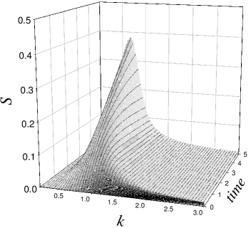
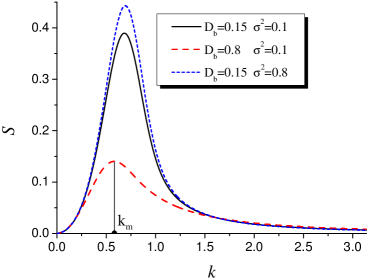
(a)                                                                  (b)

Figure 1: (Color online) The structure function for the reduced system: (a) the dynamics of $S(k,t)$ at $D_{b}=0.15$, $\sigma^{2}=0.1$; (b) the dependence $S(k)$ at a fixed time interval ($t=10$). Other parameters are: $\alpha=0.5$, $\theta=0.1$, $e=0.2$, $r_{\textrm{c}}=1$.

The linear stability analysis is valid only on a short time scale. At large time limit ($t\to\infty$), one can use the mean-field approximation based on the analysis of the solution of the Fokker-Planck equation for the probability density of the composition field.

3.2 Mean-field approximation

To analytically study the statistical properties of phase separation at $t\to\infty$ one needs to analyze a stationary probability density $\mathcal{P}_{\textrm{s}}([\psi])$. The behavior of the system can be described analytically within the framework of the mean-field approach derived for the systems with conserved dynamics [55, 56, 57, 58, 34, 35].

In the Wiess mean-field approximation, one can use the mean field (molecular field) $\eta\equiv\langle\psi\rangle$ as an order parameter for phase transitions and phase decomposition. In such a case, one uses the transformation procedure, which allows us to introduce the order parameter in $d$-dimensional space as follows:

$$\Delta\psi\equiv\rightarrow 2d(\langle\psi\rangle-\psi).$$ (3.7)

The mean-field value $\eta$ is self-consistently defined according to the definition of the mean $\langle\psi\rangle$ through the stationary distribution function $P_{\textrm{s}}$. In the mean-field theory, the stationary distribution is a function of $\psi$ and $\eta$. A procedure to obtain the corresponding distribution as a solution of the corresponding Fokker-Planck equation is shown in appendix C.

In order to define the transition and critical points at phase separation, we use the procedure proposed in references [55, 56, 59]. According to this approach in a deterministic case with $D_{b}=0$, one has a model $\partial_{t}\psi=\nabla\cdot M\nabla\delta\mathcal{F}/\delta\psi$, where the restriction $\psi_{0}=\int_{V}{\rm d}\mathbf{r}\psi(\mathbf{r},t)$ is taken into account, $\psi_{0}$ is fixed by the initial conditions. For such a system, the transition point is $\Theta_{\textrm{T}}(\psi_{0})$: at $\Theta>\Theta_{\textrm{T}}(\psi_{0})$, the homogeneous state $\psi_{0}$ is stable; at $\Theta<\Theta_{\textrm{T}}(\psi_{0})$, the system separates into two bulk phases, $\psi_{1}$ and $\psi_{2}$, fulfilling $\langle\psi\rangle=\psi_{0}$. The transition from a homogeneous state to two-phase state is critical for $\psi_{0}=0$ only, i.e. $\Theta_{\textrm{T}}(0)=\Theta_{\textrm{c}}$ is the critical point. The corresponding steady state solutions are given as solutions of the equation $\nabla M\nabla\delta\mathcal{F}/\delta\psi=0$. If no flux condition is applied, then the bounded solution is $\delta\mathcal{F}/\delta\psi=h$, where $h$ is a constant effective field (in equilibrium systems $h$ is a chemical potential). In the homogeneous case, the value $h$ depends on the initial conditions $\psi_{0}$. Above the transition point, the steady state is not globally homogeneous. Here, the system separates into two bulk phases with the values $\psi_{1}$ and $\psi_{2}$. In the case of the symmetric form of the free energy functional where two phases with $\psi_{1}=-\psi_{2}$ are realized, we get $h=0$ [55]. Hence, if the field $h$ becomes trivial, then the transition point can be defined.

By using this procedure, one finds that in the homogeneous case the mean-field is the same everywhere and equals the initial value, i.e. $\eta=\psi_{0}$. Hence, solving the self-consistency equation

$$\eta=\int\limits_{-1}^{1}\psi P_{\textrm{s}}(\psi,\eta,h){\rm d}\psi$$ (3.8)

at the fixed mean-field value, we obtain the constant effective field $h$. Below the threshold $\Theta_{\textrm{T}}$, the system decomposes into two equivalent phases with $\langle\psi_{1}\rangle=-\langle\psi_{2}\rangle$, and $h$ should be the same for these two phases and should be zero. Hence, below the threshold only $\langle\psi\rangle$ should be defined as a solution of the self-consistency equation with $P_{\textrm{s}}(\psi,\eta,0)$.

     

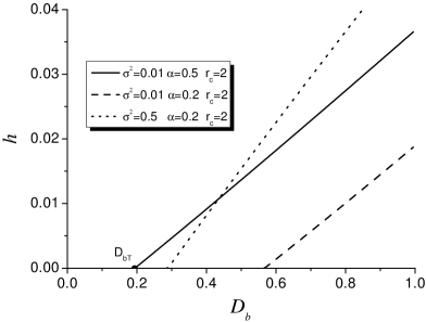
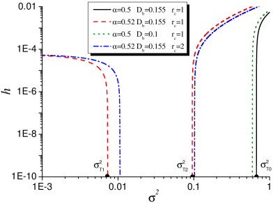
(a)                                                                (b)

Figure 2: (Color online) Constant field $h$ versus $D_{b}$ and $\sigma^{2}$ [panels (a) and (b), respectively] at $\psi_{0}=0.05$ and different sets of the system parameters.

In the actual case, we are interested in phase decomposition phenomena induced by the irradiation effect. Therefore, we define the transition and critical points only for the parameters relevant to irradiation, namely $D_{b}$, $\sigma^{2}$ by fixing $\psi_{0}$. The corresponding dependencies of the effective field $h$ versus $D_{b}$ and the external noise intensity are shown in figure 2. From figure 2 (a) it is seen that the field $h$ takes nonzero values above the transition point $D_{b\textrm{T}}$. According to the definition of $h$ as a chemical potential, one can say that at fixed $\psi_{0}$, the quantity $h$ is compensated and phase separation occurs inside the domain of the parameters where $h=0$. From the dependencies $h(D_{b})$ it follows that the ordered state with the initial concentration $\psi_{0}$ can be found only before $D_{b\textrm{T}}$. It is seen that with an increase in the strength of the dislocation mechanism described by $\alpha$, the transition point $D_{b\textrm{T}}$ decreases. Considering the dependence $h(\sigma^{2})$ [see figure 2 (b)], it follows that with an increase in $\alpha$, the phase separation processes can be realized inside the noise intensity interval $(\sigma^{2}_{\textrm{T1}},\sigma^{2}_{\textrm{T2}})$.

Next, let us discuss the mean-field $\eta$ behavior varying the system parameters. Here, we solve the self-consistency equation at $h=0$. According to figure 3 (a), the mean-field decreases with an increase in the coefficient $D_{b}$. It behaves critically in the vicinity of the value $D_{b}=D_{b\textrm{c}}$, when nontrivial values $\langle\psi_{1}\rangle=-\langle\psi_{2}\rangle$ appear. Here, we arrive at the conclusion that the irradiation leads to homogenization of the composition field distribution. By increasing the noise intensity, one finds that phase decomposition is realized at lower values of $D_{b}$ compared to the case of small $\sigma^{2}$. An increase in the intensity of internal fluctuations $\theta$ suppresses the phase separation at large $D_{b}$. The same effect can be found when the intensity of the feedback between dislocation density and composition field increases. This result follows even from the analysis of the deterministic system, where the elastic field changes the critical point position. A more interesting situation is observed by varying the external noise intensity [see figure 3 (b)]. Here, one finds that the external noise leads to the emergence of a disordered state ($\eta=0$) at $\sigma^{2}>\sigma^{2}_{\textrm{c}}$. In other words, external fluctuations of large intensity lead to a statistical disorder. On the other hand, at special choice of the system parameters related to ballistic flux properties, a reentrant behavior of the mean-field $\eta$ is observed. Here, phase decomposition is realized in a window of the noise intensity $\sigma^{2}\in[\sigma^{2}_{\textrm{c1}},\sigma^{2}_{\textrm{c2}}]$. This phenomenon is caused by the competition between regular and stochastic (correlated) parts of the ballistic flux. At $\sigma^{2}<\sigma^{2}_{\textrm{c1}}$, the most essential contribution is given by the regular component $D_{b}$ leading to homogenization of the alloy. Inside the interval $\sigma^{2}\in[\sigma^{2}_{\textrm{c1}},\sigma^{2}_{\textrm{c2}}]$, the correlation effects dominate and lead to a decrease in the effective temperature of the system. At large $\sigma^{2}$, external fluctuations destroy the ordered state. Therefore, the correlated ballistic flux is capable of inducing phase separation processes of initially homogeneous alloys. According to dependencies $h(\sigma^{2})$, one can conclude that the dislocation mechanism sustains the above reentrance.

     

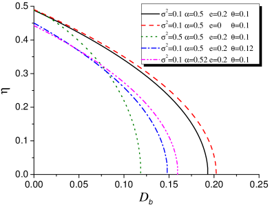
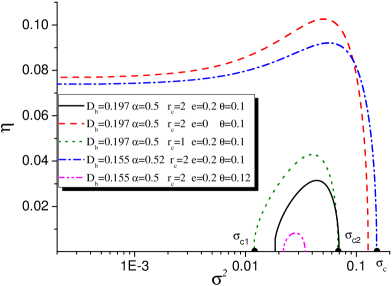
(a)                                                                (b)

Figure 3: (Color online) The mean-field value $\eta$ versus ballistic diffusion coefficient $D_{b}$ and noise intensity $\sigma^{2}$ [panels (a) and panel (b), respectively].

The corresponding phase diagram illustrating the formation of ordered and disordered phases is shown in figure 4. It is seen that a reentrant phase separation is realized in a narrow interval for $\sigma^{2}$ at elevated $D_{b}$. At small $D_{b}$, one gets the standard scenario of phase decomposition, where fluctuations suppress the ordering processes. Comparing different curves, it follows that an increase in the intensity of internal fluctuations $\theta$ shrinks the interval for the system parameters bounding the domain of the ordered phase (cf. dash and dash-dot-dot curves). The domain of reentrant ordering extends with an increase in the external noise correlation radius $r_{\textrm{c}}$ (cf. dash and dot lines). At an elevated $r_{\textrm{c}}$, the size of the domain for the ordered phase grows at small $D_{b}$. An increase in $\alpha$ shrinks the domain of the ordered phase and extends the domain of the reentrant decomposition (cf. dot and dash-dot curves).

According to the obtained results, it follows that phase separation processes can be controlled by the main system parameters (temperature and elastic properties of the alloy) and statistical properties of irradiation effect (regular and stochastic contributions in the ballistic flux). Moreover, correlated stochastic contribution of this flux is capable of inducing reentrant phase separation processes.

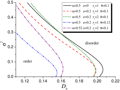
Figure 4: (Color online) The mean-field phase diagram at different sets of the system parameters.

Let us study a strong coupling limit, neglecting the spatial interactions term. Assuming $\psi=\eta$, one gets the stationary distribution in the form $P_{\textrm{s}}(\psi,\eta)=\delta(\psi-\eta)$. To obtain an equation for the effective field $h$, we integrate equation (C.27) and find

$$h=M(\eta)\left[\partial_{\eta}f(\eta)+\frac{D_{b}}{M(\eta)}\eta\right]-\frac{\theta}{2}\partial_{\eta}M(\eta)-2dD_{b}\sigma^{2}(C_{0}-C_{1})\eta.$$ (3.9)

At $h=0$, one has solutions for two bulk phases

$$\eta_{\pm}=\pm\frac{1}{2}\sqrt{4-2\alpha^{2}-2\sqrt{\alpha^{4}+4(D_{b}+\theta)-8dD_{b}\sigma^{2}(C_{0}-C_{1})}}.$$ (3.10)

The corresponding transition line can be obtained directly from equation (3.10) at $\eta=\psi_{0}$, where $\psi_{0}$ is the initial value for the composition field. Critical values for the system parameters can be obtained from the condition $\eta=0$. It is interesting to note that ballistic flux parameters lead to renormalization of the effective temperature: $\Theta$ counting off the critical one $\Theta_{\textrm{c}}=1$. Indeed, according to the definition of the free energy density $f(\psi)$ for an unirradiated system, the quantity $\Theta$ is reduced to $\alpha^{2}$. In an irradiated system, $\Theta$ is reduced to $\alpha^{2}+D_{b}+\theta-2dD_{b}\sigma^{2}(C_{0}-C_{1})$. Hence, the regular component of the ballistic flux increases the effective temperature in the same manner as the internal noise does. On the other hand, the external fluctuations reduce this temperature due to their spatial correlations. From equation (3.10) it follows that an increase in $D_{b}$, $\theta$, and $\alpha$ causes a decrease in the order parameter. The external noise is capable of extending the interval for $D_{b}$ where the mean-field takes up nonzero values.

It is known that the mean-field results are mostly qualitative. To validate the mean-field results, we will use a simulation procedure. In the next section we discuss the behavior of our system considering the dynamics of both quantities $\psi$ and $\phi$ and numerically illustrate a possibility of reentrant phase separation processes.

4 The effect of dislocation density field dynamics

4.1 Stability analysis

Considering the system with two fields $\psi$ and $\phi$, let us start with stability analysis. Averaging the system (2.5) over noises, we get dynamical equations for average fields in the form

$$\begin{split}&\partial_{t}\langle\psi\rangle=\nabla\cdot\langle M\nabla\mu_{\textrm{ef}}\rangle-\frac{\theta}{2}\nabla\cdot\left<\nabla\partial_{\psi}M\right>+\alpha\langle\phi\rangle+\sigma^{2}\left[C^{\prime\prime}(\mathbf{0})\nabla^{2}\langle\psi\rangle+C(\mathbf{0})\nabla^{4}\langle\psi\rangle\right],\\ \frac{1}{m}&\partial_{t}\langle\phi\rangle=-\langle\phi\rangle-\alpha\nabla^{2}\langle\psi\rangle+e\nabla^{2}\langle\phi\rangle\,.\end{split}$$ (4.1)

Next, let us consider the stability of the state $(\psi=0,\phi=0)$ using Lyapunov’s analysis for fluctuations of both $\psi$ and $\phi$. A linearization of the governing equations in the Fourier space yields

$$\begin{pmatrix}\frac{{\rm d}\langle\psi\rangle}{{\rm d}t}\\[4.30554pt] \frac{{\rm d}\langle\phi\rangle}{{\rm d}t}\end{pmatrix}=\begin{pmatrix}k^{2}w(k)&\alpha\\[4.30554pt] m\alpha k^{2}&-m(1+ek^{2})\end{pmatrix}\begin{pmatrix}\langle\psi\rangle\\[4.30554pt] \langle\phi\rangle\end{pmatrix},$$ (4.2)

where

$$w(k)=\alpha^{2}-1+\theta+D_{b}\left[1+\sigma^{2}C^{\prime\prime}(0)\right]+\left[1-D_{b}\sigma^{2}C(0)\right]k^{2}.$$ (4.3)

The corresponding Lyapunov exponent takes the form

$$2\lambda=\left[k^{2}w(k)-m\left(1+ek^{2}\right)\right]\pm\sqrt{\left[k^{2}w(k)+m\left(1+ek^{2}\right)\right]^{2}+4m\left[1+k^{2}w(k)+\left(e+\alpha^{2}\right)k^{2}\right]}.$$ (4.4)

According to the analysis of the Lyapunov exponent (4.4), we can find critical values for $D_{b}$ and $\sigma^{2}$, bounding the domain of unstable modes. The corresponding stability diagram is shown in figure 5 (a). It is seen that spatial instability characterized by $\lambda(k)>0$ is possible only inside the window for the ballistic diffusion coefficient. At the same time, a growth in $D_{b}$ shrinks the interval for $\sigma^{2}$ where $\lambda(k)>0$. From the stability diagram, one finds that at small $D_{b}$, the external noise can sustain a spatial instability even at large intensities of fluctuations. An increase in the correlation radius $r_{\textrm{c}}$ of these fluctuations enlarges the instability domain. Therefore, strongly correlated external fluctuations are capable of inducing spatial instability at short time scales. As figure 5 (b) shows, the critical wave-number bounding wave-number of unstable modes decreases with $D_{b}$ and $\sigma^{2}$. Therefore, at a large ballistic mixing intensity and the intensity of external fluctuations, long-wave spatial instabilities should emerge over the whole system.

     

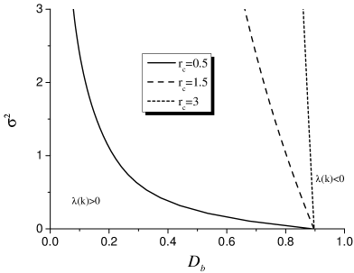
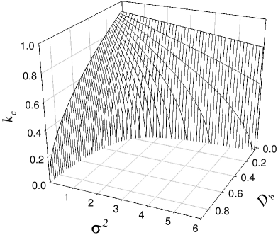
(a)                                                          (b)

Figure 5: Stability diagram (a) and critical wave-number dependence on $D_{b}$ and $\sigma^{2}$ (b) at $m=1$, $\alpha=0.5$, $r_{\textrm{c}}=0.5$.

Let us consider the behavior of the structure function $S(k,t)$. To obtain a dynamical equation for $S(k,t)$ in the vicinity of the point $(\psi=0,\phi=0)$, we exploit the approach previously described by considering the system of two equations (2.5). Moving to the discrete representation and multiplying every equation from the system (2.5) by $\psi$, we arrive at the system of two equations

$$\begin{split}\frac{{\rm d}S(k,t)}{{\rm d}t}=&-2k^{2}w(k)S(k,t)+\alpha G(k,t)+2\theta k^{2}-\frac{2k^{2}}{(2\pi)^{2}}\int{\rm d}\mathbf{q}S(q,t)+\frac{2k^{2}D_{b}\sigma^{2}}{(2\pi)^{2}}\int{\rm d}\mathbf{q}C(|\mathbf{k}-\mathbf{q}|)S(\mathbf{q},t),\\ \frac{{\rm d}G(k,t)}{{\rm d}t}=&-2m\left[\left(1+ek^{2}\right)G(k,t)-\alpha k^{2}S(k,t)\right],\end{split}$$ (4.5)

where $G(k,t)\equiv\langle\psi_{\mathbf{k}}(t)\phi_{-\mathbf{k}}(t)\rangle=\langle\psi_{-\mathbf{k}}(t)\phi_{\mathbf{k}}(t)\rangle$, and $w(k)$ is given by equation (4.3).

The dynamics of $S(k,t)$ is shown in figure 6 (a). Comparing graphs for $S(k,t)$ related to actual and reduced models [cf. figures 6 (a), 1 (a)], one finds that the peak of the structure function is larger in the actual two-component dynamical model. From the obtained dependencies for the structure function $S(k)$ shown in figure 6 (b) it is seen that an increase in the regular component of the ballistic flux essentially decreases the structure function; it shifts the peak position toward small wave-numbers. Considering the effect of the dislocation density mechanism strength, one finds that with an increase in $\alpha$, the wave-number of unstable modes decreases [see the insertion in figure 6 (b)]. At the same time, the height of the peak of the structure function decreases at a short time scale. Therefore, the dislocation mechanism is capable of delaying the ordering processes. Herein below, we will show that this effect can be observed by the dynamics of the average domain size.

     

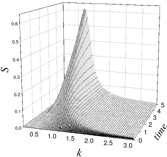
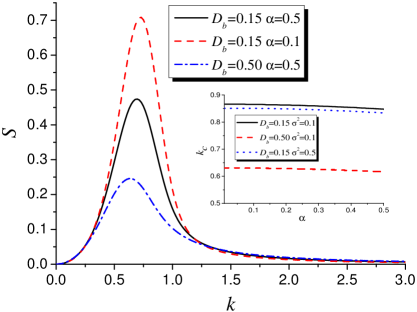
(a)                                                                  (b)

Figure 6: (Color online) The structure function behavior for the original system: a) the dynamics of $S(k,t)$ at $D_{b}=0.15$, $\sigma^{2}=0.1$; b) the dependence $S(k)$ at $t=10$ and a different set of the system parameters. Other parameters are: $\theta=0.1$, $\alpha=0.5$, $e=0.2$, $r_{\textrm{c}}=1.0$, $m=1.0$.

4.2 Numerical results

To qualitatively describe the system behavior, we numerically solve the system (2.5). In simulation procedure, the Heun method was used. The system was studied on the lattice with square symmetry of the linear size $L=128\ell$ with periodic boundary conditions and the mesh size $\ell=0.5$; $\Delta t=0.005$ is the time step. We take $\langle\psi(\mathbf{0},0)\rangle=\langle\phi(\mathbf{0},0)\rangle=0$, $\langle(\delta\psi(\mathbf{0},0))^{2}\rangle=\langle(\delta\phi(\mathbf{0},0))^{2}\rangle=0.01$ as initial conditions. The obtained results are statistically independent of different realizations of noise terms $\zeta$, $\xi$.

Typical evolution of both the composition field $\psi$ and dislocation density $\phi$ is shown in figure 7. Here, the regions of high values of both fields $\psi$ and $\phi$ are represented by white, whereas the black areas relate to lower values of the corresponding field. The coupling between dislocation density and composition field is well observed. A coordinated motion of dislocations and phase boundaries was previously observed at atomic scale using phase field models (see references [28, 60])

It is seen that the dislocation field takes up large values in the vicinity of the phase boundaries; inside the decomposed phases, the dislocation density is around zero. The corresponding oscillations of $\psi$ near the interfaces indicate that the strain energy is reduced due to the atomic size mismatch [28]. Therefore, misfit dislocations segregate on the boundaries. In figure 8, we plot the oscillating structure of dislocation density field $\phi$ corresponding to the distribution of the concentration field. It is seen that in the vicinity of the boundary, $\phi$ changes the sign; inside the phases, $\phi\simeq 0$.

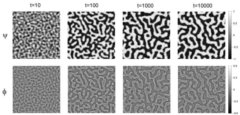
Figure 7: Evolution of both the composition field $\psi$ (top panels) and dislocation field (bottom panels) at $D_{b}=0.15$, $\sigma^{2}=0.5$, $\theta=0.1$, $\alpha=0.5$, $e=0.2$, $r_{\textrm{c}}=1.0$, $m=1$.

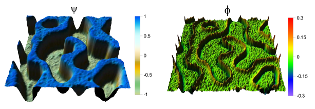
Figure 8: (Color online) Snapshots of both concentration and dislocation fields at $t=10000$ shown in 3D-view, illustrating the oscillating behavior of dislocation density field near the boundaries of two phases $\psi=+1$ and $\psi=-1$. Other parameters are: $D_{b}=0.15$, $\sigma^{2}=0.1$, $\theta=0.01$, $\alpha=0.5$, $e=0.2$, $r_{\textrm{c}}=1.0$, $m=10$.

To make a quantitative analysis of phase separation, let us study the dependencies of dispersions of the fields $\psi$ and $\phi$ defined as $J_{\psi}\equiv\langle(\delta\psi)^{2}\rangle$ and $J_{\phi}\equiv\langle(\delta\phi)^{2}\rangle$, where $\delta\psi=\psi-\langle\psi\rangle$, $\delta\phi=\phi-\langle\phi\rangle$. At $\langle\psi\rangle=\langle\phi\rangle=0$, these quantities are reduced to the second statistical moments playing the role of effective order parameters at phase decomposition processes (due to conservation laws for $\psi$ and $\phi$). The quantity $J_{\psi}(t)$ is proportional to the area below the structure function $S_{k}(t)$, i.e., $J_{\psi}(t)=\sum_{k}S_{k}(t)$. Therefore, the growth in $J_{\psi}$ (and the related growth of $J_{\phi}$) corresponds to the phase decomposition process. Both moments $J_{\psi}$ and $J_{\phi}$ grow toward nonzero stationary values. The related stationary values $J_{\{\psi,\phi\}}^{\textrm{st}}=J_{\{\psi,\phi\}}(t\to\infty)$ can be used to define two phases separated during the the long time evolution of the system. If dislocations are excluded from the description, then one can use only $J_{\psi}$ to monitor the formation of two phases. In our case, the dynamics of phase decomposition can be described by an additional order parameter $J_{\phi}$ manifesting segregation of dislocations in the vicinity of the interface. From naive consideration, one can expect that at large values of both $J_{\psi}$ and $J_{\phi}$, one gets two well decomposed phases with an increased dislocation density at the interface. At small $J_{\psi}$ and $J_{\phi}$, one gets a mixed state where no large deviations in the composition field are observed. On the other hand, it means that dislocations are distributed inside the phases.

In figure 9, we plot the dependencies of the order parameters at different values of the external noise intensity at other fixed system parameters. It is seen that an increase in the noise intensity $\sigma^{2}$ results in small values of both $J_{\psi}$ and $J_{\phi}$. At $\sigma^{2}=0$ (see solid lines in figure 9), the order parameter $J_{\psi}$ grows toward stationary value in a monotonous manner. This means an increase in the area under the corresponding structure function $S(k,t)$ and the formation of well decomposed phases enriched by atoms of different sorts (see right-hand panel illustrating the distribution of the composition field $\psi$). The order parameter $J_{\phi}$ initially grows meaning the formation of two separated phases with an increasing dislocation density in the vicinity of the interface. At the next stage, a decaying dependence of $J_{\phi}$ is observed. This means an agglomeration of the domains belonging to one phase resulting in annihilations of dislocations with opposite signs. At the late stage, the dislocation density goes to its stationary value together with $J_{\psi}$. At a small noise intensity $\sigma^{2}$ (see dashed curves in figure 9), one observes the same dynamics of both order parameters, where $J_{\psi}$ and $J_{\phi}$ take up low values. Here, the external noise sustains the formation of an ordered state characterized by separated phases. This effect is caused by correlation properties of the external noise. The deterministic part of the ballistic flux acts in the manner opposite to the stochastic contribution. By increasing the noise intensity $\sigma^{2}$ (in the domain of a disordered phase according to the mean-field analysis), one gets a transition toward disordered state. Here the order parameter $J_{\psi}$ attains a very small stationary value (see dotted curves in figure 9). The formation of a disordered state is well accompanied by time independence of the quantity $J_{\phi}$. It fastly attains a small stationary value and fluctuates around it. Here, there are no phases enriched by atoms A or B (see the right-hand panel in figure 9), dislocations are distributed over the whole system. Therefore, the effect of fluctuations characterized by large values of $\sigma^{2}$ becomes larger than the correlation effects, leading to the formation of a totally disordered state.

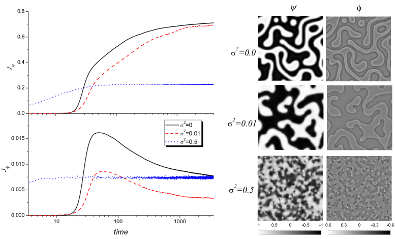
Figure 9: (Color online) The dynamics of both order parameters $J_{\psi}$ and $J_{\phi}$ at different values of the external noise intensity $\sigma^{2}$, and the corresponding snapshots of both concentration and dislocation density fields at $t=4000$. Other parameters are: $D_{b}=0.15$, $\theta=0.01$, $\alpha=0.5$, $e=0.2$, $r_{\textrm{c}}=2.0$, $m=10$.

Let us consider in detail the effect of the dislocation density field onto the dynamics of the phase decomposition. An evolution of both order parameters $J_{\psi}$ and $J_{\phi}$ at different values of the coupling constant $\alpha$ is shown in figure 10 (a). Here, one can see that both $J_{\psi}$ and $J_{\phi}$ increase with $\alpha$ (the order parameter $J_{\phi}$ has the corresponding peak at transition to the coarsening regime). Let us consider the behavior of the stationary order parameter $J^{\textrm{st}}_{\psi}=J_{\psi}(t\to\infty)$ [see the insertion in the upper panel in figure 10 (a)]. It rapidly increases at small $\alpha$ and slowly grows with $\alpha$. From the obtained results it follows that a strong coupling between the composition field and the dislocation density field urges the formation of the ordered state due to redistribution of dislocations over the whole system, as well as their motion to the interfaces. Therefore, phase separation is well sustained by a dislocation field. It is interesting to compare the dynamics of the average domain size at different $\alpha$. According to discussions provided in references [38, 39] it is known that dislocation mechanism is capable of changing the dynamical exponent $z$, describing the domain size growth law $\langle R\rangle\propto t^{z}$. To analyze the dependence $\langle R(t)\rangle$, we calculate the averaged value $\langle k(t)\rangle\propto 1/\langle R(t)\rangle$ according to the standard definition $\langle k(t)\rangle=\int kS(k,t){\rm d}k/\int S(k){\rm d}k$. In the standard theory of phase decomposition, the corresponding Lifshitz-Slyozov approach gives $z=1/3$ [61]. The same value for $z$ is observed when phase separation is sustained by vacancy mechanism. If dislocation mechanism of phase decomposition plays the major role, then the dynamical exponent takes up lower values $z\simeq 1/6$ [39]. In our case, we can control the strength of the dislocation mechanism varying parameter $\alpha$. According to the results in figure 10 (b), one obtains $z\simeq 0.33$ at $\alpha\to 0$, as Lifshitz-Slyozov theory predicts. This result was obtained for the system subjected to a stochastic ballistic flux with another form of the function $\tilde{M}(\psi)$ (see reference [34]). It was shown that an increase in the external noise intensity $\sigma^{2}$ results in disordering processes. Comparing the curves related to $\alpha=0.1$ and $\alpha=0.5$, it follows that the dislocation mechanism delays the dynamics of the domain sizes growth. In our case, at $\alpha=0.5$, we get a lower value for the dynamical exponent.

     

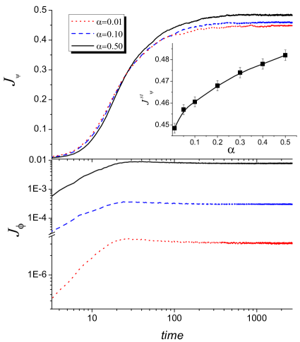
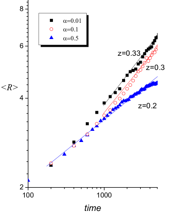
(a)                                                          (b)

Figure 10: (Color online) (a) Dynamics of both order parameters $J_{\psi}$ and $J_{\phi}$ at different $\alpha$ and $D_{b}=0.12$, $\sigma^{2}=0.01$. (b) Evolution of the average domain size at different $\alpha$ and $D_{b}=0.1$, $\sigma^{2}=0.5$. Other parameters are: $\theta=0.01$, $e=0.2$, $r_{\textrm{c}}=2.0$, $m=10$.

Finally, let us consider the dynamics of the average dislocation density $\langle\phi_{H}\rangle$ in the vicinity of the interfaces and the coherence (interface) width $\langle L_{\phi}\rangle$, where this density decreases toward zero value inside the separated phases. We calculate the quantity $\langle\phi_{H}\rangle$ as the mean height of $\phi(\mathbf{r})$ profile averaged over the whole system. The coherence width $\langle L_{\phi}\rangle$ is calculated as the width of the interface on the half-height of $\phi(\mathbf{r})$ profile averaged over the system. In figure 11 (a), solid and dashed lines denote one-dimensional profiles for the composition and dislocation density fields, respectively. The dynamics of both $\langle\phi_{H}\rangle$ and $\langle L_{\phi}\rangle$ is shown in figure 11 (b). Comparing the data related to different sets of $D_{b}$ and $\sigma^{2}$, one finds that the dislocation density attains a stationary value during the decomposition process. Considering the dynamics of $\langle\phi_{H}\rangle$ at different external noise intensities, it follows that the growth in $\sigma^{2}$ increases the values of the dislocation density. Therefore, the external noise is capable of inducing a phase decomposition accompanied by segregation of dislocations at interfaces. On the other hand, with an increase in $D_{b}$, the quantity $\langle\phi_{H}\rangle$ takes up lower values. Here, dislocations are distributed over the whole system due to homogenization of the system produced by a regular component of the ballistic flux. The competition between regular and stochastic components of the ballistic flux can be observed by studying the dynamics of the averaged interface width. From the bottom panel in figure 11 (b), one finds that during the system evolution, the quantity $\langle L_{\phi}\rangle$ attains a maximum. This maximum relates to the stage of the domains growth. A coalescence regime (large domains absorb small ones) is accompanied here by an increase in the interface width. A decrease in $\langle L_{\phi}\rangle$ corresponds to a coarsening regime. At large time intervals, $\langle L_{\phi}\rangle$ attains a stationary value. Comparing the corresponding stationary values at different $D_{b}$, it follows that a regular component of the ballistic flux produces a disordering accompanied by extension of the interface width (cf. the curves marked by circles and triangles). Comparing the curves with different $\sigma^{2}$, one finds that the noise is capable of playing a constructive role leading to a decrease in the interface width. Localization of dislocations at interfaces can be stimulated by a correlation effect of the external fluctuations [see the curve with triangles in the upper panel in figure 11 (b)]. It should be noted that the above effect is possible only inside the domain of the ordered phase formation. Therefore, the mentioned above constructive role of external fluctuations is caused by their spatial correlations.

  

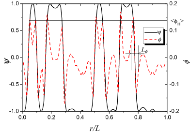
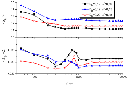
(a)                                                                  (b)

Figure 11: (Color online) (a) Illustration of typical one-dimensional profiles for solute concentration $\psi$ and the field $\phi$ taken at the time $t=400$ ($D_{b}=0.12$, $\sigma^{2}=0.1$). (b) Evolution of both the average maximum dislocation density field $\langle\phi_{H}\rangle$ and a coherence length $\langle L_{\phi}\rangle$ at different values of $D_{b}$ and $\sigma^{2}$. Other parameters are: $\alpha=0.5$, $e=0.2$, $r_{\textrm{c}}=1$, $m=1$, $\theta=0.1$.

5 Conclusions

We have studied phase separation processes driven by the dislocation evolution mechanism in a binary system subjected to sustained irradiation. We describe the irradiation effect by introducing a ballistic flux having stochastic properties. We assumed that these fluctuations are spatially correlated.

By taking into account different time scales of evolution of both composition and dislocation density fields, we have initially considered a reduced model using the adiabatic elimination procedure. In this case, the dynamics of the composition field playing the role of a slow mode is studied. By making use of the linear stability analysis, we have shown the constructive role of ballistic flux fluctuations. These fluctuations induce spatial instability at a short time scale. At a large time scale, we have used the mean-field approach allowing us to describe the properties of phase separation. Corresponding mean-field phase diagrams illustrating the possibility of phase decomposition are calculated. It was found that ballistic flux components reduced to the intensity of atomic mixing (ballistic diffusion coefficient) and the intensity of the corresponding fluctuations are capable of controling reentrant phase separation processes. It was shown that a reentrant character of phase separation is governed by spatial correlations of the external noise and mobile dislocations.

Considering the dynamics of both studied fields by means of computer simulations, we have found that the formation of domains enriched by atoms of different sort is accompanied by an increase of the dislocation density field in the vicinity of the interface. Inside such domains, dislocation density takes up zero values and all dislocations characterized by different signs in two phases segregate on interfaces. The average length of the interface decreases at the formation of the ordered state. In the disordered state, all dislocations are distributed over the whole system. It was shown that spatially correlated external fluctuations act in the manner opposite to the regular component of the ballistic flux and induce the ordered state formation. Studying the effect of the dislocation density field onto phase decomposition we have considered the dynamics of the average domain size at different strengths of the dislocation mechanisms. It was shown that the universal dynamics of the average domain size delays due to a redistribution of dislocations. We have found that at small contribution of the dislocation density field, the corresponding universal dynamics is described by the standard Lifshitz-Slyozov law with dynamical exponent $z=0.33$. With an increase in the dislocation mechanism strength, this exponent takes up lower values and the domains of new phases are characterized by smaller linear sizes.

Appendix A

Let us represent the system on a regular $d$-dimension lattice. Within the framework of the standard formalism of a discrete representation, the system can be divided onto $N^{d}$ cells of the linear size $L=\ell N$, where $\ell$ is the a mesh size. Then, the partial differential equation (3.1) is reduced to a set of usual differential equations written for every cell $i$ on a grid in the form

$$\frac{{\rm d}\psi_{i}}{\rm{d}t}=\nabla^{\textrm{L}}_{ij}\tilde{M}_{j}\nabla^{\textrm{R}}_{jl}\tilde{\mu}_{l}+\nabla^{\textrm{L}}_{ij}\sqrt{\tilde{M}_{j}}\xi_{j}(t)+\nabla^{\textrm{L}}_{ij}\nabla^{\textrm{R}}_{jk}\psi_{k}\zeta_{k}(t),$$ (A.1)

where the index $i$ labels cells, $i=1,\ldots,N^{d}$; the discrete left-hand and right-hand operators are:

$$\begin{split}&\nabla^{\textrm{L}}_{ij}=\frac{1}{\ell}(\delta_{i,j}-\delta_{i-1,j}),\qquad\nabla^{\textrm{R}}_{ij}=\frac{1}{\ell}(\delta_{i+1,j}-\delta_{i,j}),\\ &\nabla^{\textrm{L}}_{ij}=-\nabla^{\textrm{R}}_{ji},\qquad\qquad\qquad\nabla^{\textrm{L}}_{ij}\nabla^{\textrm{R}}_{jl}=\Delta_{il}=\frac{1}{\ell^{2}}(\delta_{i,l+1}-2\delta_{i,l}+\delta_{i,l-1}).\end{split}$$ (A.2)

Discrete correlators of stochastic sources are of the form:

$$\langle\xi_{i}(t)\xi_{j}(t)\rangle=\ell^{-2}\theta\delta_{ij}\delta(t-t^{\prime}),\qquad\langle\zeta_{i}(t)\zeta_{j}(t)\rangle=D_{b}\sigma^{2}C_{i-j}\delta(t-t^{\prime}),$$ (A.3)

where $C_{i-j}$ is the discrete representation of the spatial correlation function $C(\mathbf{r})$ which in the limit of zero correlation length becomes $\delta_{ij}/\ell^{d}$. For the two-dimensional problem considered below, the quantity $C_{|i-j|}$ can be computed as a discrete version of the Fourier transform of $C(\mathbf{r}-\mathbf{r}^{\prime})$ written in the form [53] $C(k)=\exp\left\{-({r_{\textrm{c}}^{2}}/{2})[\sin^{2}(k_{x}/2)+\sin^{2}(k_{y}/2)]\right\}$. Noise correlators can be calculated according to the recipes shown in references [53, 54, 58, 34]. Next, we consider the case $d=2$.

To calculate the internal noise correlator $\langle\sqrt{M}\xi\rangle$, we use the Novikov theorem which can be written in the form

$$\left\langle\sqrt{\tilde{M}_{i}}\xi_{i}(t)\right\rangle=\sum_{j}\int_{0}^{t}\left\langle\xi_{i}(t)\xi_{j}(t^{\prime})\right\rangle\left\langle\frac{\delta\sqrt{\tilde{M}_{i}}}{\delta\xi_{j}(t^{\prime})}\right\rangle{\rm d}t^{\prime}=\frac{\theta}{\ell^{2}}\int_{0}^{t}\left\langle\left.\frac{\delta\sqrt{\tilde{M}_{i}}}{\delta\xi_{i}(t^{\prime})}\right|_{t=t^{\prime}}\right\rangle{\rm d}t^{\prime}.$$ (A.4)

Using a relation

$$\left.\frac{\delta\sqrt{\tilde{M}_{i}}}{\delta\xi_{i}(t^{\prime})}\right|_{t=t^{\prime}}=\left.\frac{{\rm d}\sqrt{\tilde{M}_{i}}}{{\rm d}\psi_{i}(t)}\frac{\delta\psi_{i}(t)}{\delta\xi_{i}(t^{\prime})}\right|_{t=t^{\prime}}$$

and a formal solution of the Langevin equation (A.1), one can write

$$\left.\frac{\delta\psi_{i}(t)}{\delta\xi_{i}(t^{\prime})}\right|_{t=t^{\prime}}=\nabla^{\textrm{L}}_{ij}\sqrt{\tilde{M}_{j}}\,.$$

Substituting it into equation (A.4), we get

$$\left\langle\sqrt{\tilde{M}_{i}}\xi_{i}(t)\right\rangle=\frac{\theta}{\ell^{2}}\nabla^{\textrm{L}}_{ij}\left\langle\frac{{\rm d}\sqrt{\tilde{M}_{j}}}{{\rm d}\psi_{j}}\sqrt{\tilde{M}_{j}}\right\rangle=\frac{\theta}{2{\ell^{2}}}\nabla^{\textrm{L}}_{ij}\left\langle\frac{{\rm d}\tilde{M}_{j}}{{\rm d}\psi_{j}}\right\rangle.$$ (A.5)

Using the relation between left-hand and right-hand discrete gradient operators and moving to the continuum limit, we get

$$\nabla\cdot\left\langle\sqrt{\tilde{M}}\xi\right\rangle=-\frac{\theta}{2}\nabla\cdot\left\langle\nabla\partial_{\psi}\tilde{M}\right\rangle.$$ (A.6)

To calculate the external noise correlator $\langle\psi\zeta\rangle$, we again use the Novikov theorem written as follows:

$$\langle\psi_{j}\zeta_{j}(t^{\prime})\rangle=\sum_{k}\int_{0}^{t}\langle\zeta_{j}(t)\zeta_{k}(t^{\prime})\rangle\left\langle\frac{\delta\psi_{j}(t)}{\delta\zeta_{j}(t^{\prime})}\right\rangle{\rm d}t^{\prime}=D_{b}\sigma^{2}\sum_{k}C_{j-k}\left\langle\left.\frac{\delta\psi_{j}(t)}{\delta\zeta_{k}(t^{\prime})}\right|_{t=t^{\prime}}\right\rangle.$$ (A.7)

According to the formal solution of the Langevin equation, the corresponding derivative with respect to $\zeta$ takes the form $\left<\delta\psi_{j}/\delta\zeta_{k}|_{t=t^{\prime}}\right>=\Delta_{jk}\left<\psi_{k}\right>$. Next, substituting it into equation (A.7) and using a discrete representation of the Laplacian, we find the sum over the index $k$ allowing us to write

$$\langle\psi_{j}\zeta_{j}\rangle=\frac{D_{b}\sigma^{2}}{\ell^{2}}\left[C_{1}\langle\psi_{j+1}\rangle+C_{-1}\langle\psi_{j-1}\rangle-2C_{0}\langle\psi_{j}\rangle\right].$$ (A.8)

Acting by Laplacian operator onto this construction, we finally obtain in continuum limit

$$\Delta\langle\psi\zeta\rangle=D_{b}\sigma^{2}\left[C(\mathbf{0})\nabla^{4}\langle\psi\rangle+C^{\prime\prime}(\mathbf{0})\Delta\langle\psi\rangle\right].$$ (A.9)

Appendix B

To obtain a dynamical equation for the structure function, we need to construct a dynamical equation for the two-point correlation function $\langle\psi_{i}\psi_{j}\rangle$. In our computation procedure, we use the procedure described in reference [62]. Multiplying the linearized Langevin equation (A.1) written for $\psi_{j}$ onto $\psi_{i}$ and doing the same procedure for the linearized Langevin equation written for $\psi_{i}$, we add these two equations. This procedure allows us to obtain a dynamical equation for $\langle\psi_{i}\psi_{j}\rangle$ written in the form

$$\frac{{\rm d}\langle\psi_{i}\psi_{j}\rangle}{{\rm d}t} = \Delta_{ik}\left[\left(D_{b}-1+\alpha^{2}\right)\langle\psi_{j}\psi_{k}\rangle-\left(1-\alpha^{2}e\right)\Delta_{kl}\langle\psi_{l}\psi_{j}\rangle+\langle\psi_{j}\psi_{k}\zeta_{k}\rangle\right]$$ (B.10)

$$+ \langle\psi_{i}\nabla^{\textrm{L}}_{jk}\xi_{k}\rangle-2\langle\psi_{i}\nabla^{\textrm{L}}_{jk}\psi_{k}\xi_{k}\rangle$$

$$+ \Delta_{jk}\left[\left(D_{b}-1+\alpha^{2}\right)\langle\psi_{i}\psi_{k}\rangle-\left(1-\alpha^{2}e\right)\Delta_{kl}\langle\psi_{l}\psi_{i}\rangle+\langle\psi_{i}\psi_{k}\zeta_{k}\rangle\right]$$

$$+ \langle\psi_{j}\nabla^{\textrm{L}}_{ik}\xi_{k}\rangle-2\langle\psi_{j}\nabla^{\textrm{L}}_{ik}\psi_{k}\xi_{k}\rangle,$$

where the sum runs over the repeating indexes. Using the Novikov theorem with recipe shown in Appendix A, one can calculate the following correlators:

$$\begin{split}&\langle\psi_{i}\nabla^{\textrm{L}}_{jk}\xi_{k}\rangle=-\frac{\theta}{\ell^{2}}\Delta_{ij}\,,\qquad\langle\psi_{i}\nabla^{\textrm{L}}_{jk}\psi_{k}\xi_{k}\rangle=-\frac{\theta}{2\ell^{2}}\left(\Delta_{jk}\langle\psi_{k}\psi_{j}\rangle+\Delta_{ik}\langle\psi_{k}\psi_{j}\rangle\right),\\ &\langle\psi_{j}\psi_{k}\zeta_{k}\rangle=D_{b}\sigma^{2}\left(\Delta_{kl}C_{k-l}\langle\psi_{l}\psi_{j}\rangle+\Delta_{jl}C_{k-l}\langle\psi_{l}\psi_{k}\rangle\right).\end{split}$$ (B.11)

Introducing the structure function $S(\mathbf{k},t)\equiv\langle\psi_{\mathbf{k}}(t)\psi_{-\mathbf{k}}(t)\rangle$ in the discrete space

$$S_{\nu}(t)=(N\ell)^{-2}\langle\psi_{\nu}(t)\psi_{-\nu}(t)\rangle$$

with Fourier components

$$\psi_{\nu}(t)=\ell^{2}\sum_{m}\mathrm{e}^{-\mathrm{i}\mathbf{r}_{m}\mathbf{k}_{\nu}}\psi_{m}(t),\qquad\psi_{m}(t)=(N\ell)^{-2}\sum_{\nu}\mathrm{e}^{\mathrm{i}\mathbf{r}_{m}\mathbf{k}_{\nu}}\psi_{\nu}(t)$$

one can define the derivative

$$\frac{{\rm d}S_{\nu}}{{\rm d}t}=(\ell/N)^{2}\mathrm{e}^{\mathrm{i}\mathbf{k}_{\nu}(\mathbf{r}_{j}-\mathbf{r}_{m})}\frac{{\rm d}\langle\psi_{m}\psi_{j}\rangle}{{\rm d}t}.$$

In the following computations, one needs to exploit definitions:

$$\left(\frac{\ell}{N}\right)^{2}\mathrm{e}^{\mathrm{i}\mathbf{k}_{\nu}(\mathbf{r}_{j}-\mathbf{r}_{i})}\Delta_{is}\langle\psi_{s}\psi_{j}\rangle=\widehat{D}_{\nu}S_{\nu}(t),$$ (B.12)

$$\Delta_{is}\langle\psi_{s}\psi_{j}\rangle=(N\ell)^{-4}\mathrm{e}^{\mathrm{i}\mathbf{k}_{\nu}\mathbf{r}_{j}}\mathrm{e}^{\mathrm{i}\mathbf{k}_{\mu}\mathbf{r}_{i}}\widehat{D}_{\mu}\langle\psi_{\mu}\psi_{\nu}\rangle,$$ (B.13)

$$2\left(\frac{\ell}{N}\right)^{2}\mathrm{e}^{\mathrm{i}\mathbf{k}_{\nu}(\mathbf{r}_{j}-\mathbf{r}_{i})}C_{|i-j|}\langle\psi_{i}\psi_{j}\rangle=(N\ell)^{-2}\sum_{\mu}C_{\mu}S_{\mu-\nu}(t),$$ (B.14)

where $\widehat{D}_{\nu}=\ell^{-2}\big{(}\sum_{|i|=1}\cos(\mathbf{k}_{\nu}\mathbf{r}_{i})-1\big{)}$ can be understood as the Fourier transform of the discrete Laplacian. Using the above definitions and equation (B.10) with correlators (B.11), we arrive at the equation for the quantity $S_{\nu}(t)$:

$$\frac{{\rm d}S_{\nu}(t)}{{\rm d}t} = 2\widehat{D}_{\nu}\left[\alpha^{2}-1+\theta+D_{b}+D_{b}\sigma^{2}\Delta_{0m}C_{m}-\widehat{D}_{\nu}\left(1-D_{b}\sigma^{2}C_{1}\right)\right]S_{\nu}(t)$$ (B.15)

$$- 2\theta\widehat{D}_{\nu}+2\widehat{D}_{\nu}(N\ell)^{-2}\sum_{\mu}S_{\mu}(t)-2D_{b}\sigma^{2}(N\ell)^{-2}\widehat{D}_{\nu}\sum_{\mu}C_{\nu-\mu}S_{\mu}(t).$$

In continuous and thermodynamical limit ($N\to\infty$, $\ell\to 0$), we obtain a dynamical equation for the structure function in the form

$$\frac{{\rm d}S(k,t)}{{\rm d}t} = -2k^{2}\left\{\alpha^{2}-1+\theta+D_{b}(1+\sigma^{2}C^{\prime\prime}(0))+k^{2}\left[1-\alpha^{2}e-D_{b}\sigma^{2}C(0)\right]\right\}S(k,t)$$ (B.16)

$$+ 2\theta k^{2}-\frac{2k^{2}}{(2\pi)^{2}}\int{\rm d}\mathbf{q}S(q,t)+\frac{2k^{2}D_{b}\sigma^{2}}{(2\pi)^{2}}\int{\rm d}\mathbf{q}C(|\mathbf{k}-\mathbf{q}|)S(\mathbf{q},t).$$

Appendix C

To obtain the probability density distribution $\mathcal{P}([\psi],t)$ in $d$-dimensional space, let us start with definitions:

$$\mathcal{P}([\psi],t)=\left\langle\prod\limits_{i=1}^{N^{d}}\rho_{i}(t)\right\rangle\equiv\left\langle\rho(t)\right\rangle,\quad\rho_{i}(t)=\overline{\delta(\psi_{i}(t)-\psi_{i})}_{\textrm{IC}}\,,$$ (C.17)

where $\ldots_{\textrm{IC}}$ and $\langle\ldots\rangle$ are the averages over initial conditions and fluctuations, respectively. To obtain the corresponding Fokker-Planck equation, we use a standard technique and exploit the stochastic Liouville equation for the distribution $\rho(t)$ in the form

$$\partial_{t}\rho=-\frac{\partial}{\partial\psi_{i}}(\dot{\psi}_{i}\rho).$$ (C.18)

Inserting the expression for the time derivative from equation (A.1) and averaging over the noise, we get

$$\partial_{t}\mathcal{P}=-\frac{\partial}{\partial\psi_{i}}\left(\nabla^{\textrm{L}}_{ij}M_{j}\nabla^{\textrm{R}}_{jl}\tilde{\mu}_{l}\right)\mathcal{P}-\frac{\partial}{\partial\psi_{i}}\left(\langle\nabla^{\textrm{L}}_{ij}\sqrt{M_{j}}\xi_{j}(t)\rho\rangle+\langle\Delta_{ij}\psi_{j}\zeta_{j}(t)\rho\rangle\right).$$ (C.19)

Correlators in the second term can be calculated by means of the Novikov theorem, that at $\ell=1$ gives [52]

$$\begin{split}&\left\langle\nabla^{\textrm{L}}_{ij}\sqrt{M_{j}(t)}\xi_{j}(t)\rho\right\rangle=\theta\int\limits_{0}^{t}{\rm d}t^{\prime}\delta_{jk}\delta(t-t^{\prime})\left\langle\frac{\delta\nabla^{\textrm{L}}_{ij}\sqrt{M_{j}(t)}\rho}{\delta\xi_{k}(t^{\prime})}\right\rangle,\\ &\qquad\langle\Delta_{ij}\psi_{j}\zeta_{j}(t)\rho\rangle=D_{b}\sigma^{2}\int\limits_{0}^{t}{\rm d}t^{\prime}C_{|j-k|}\delta(t-t^{\prime})\left\langle\frac{\delta\Delta_{ij}\psi_{j}\rho}{\delta\zeta_{k}(t^{\prime})}\right\rangle.\end{split}$$ (C.20)

Introducing notations $g_{ij}=\{(\nabla_{L})_{ij}\sqrt{M_{j}},\Delta_{ij}\psi_{j}\}$, $\lambda=\{\xi,\zeta\}$, for the last multiplier, one has

$$\frac{\delta g_{ij}\rho(t)}{\delta\lambda_{k}(t^{\prime})}=-\sum_{l}g_{ij}\frac{\partial}{\partial\psi_{k}}\frac{\delta\psi_{l}(t)}{\delta\lambda_{k}(t^{\prime})}\bigg{|}_{t=t^{\prime}}\rho.$$ (C.21)

Using a formal solution of the Langevin equation, the response functions take up the form

$$\left.\frac{\delta\psi_{l}(t)}{\delta\xi_{k}(t^{\prime})}\right|_{t=t^{\prime}}=\nabla^{\textrm{L}}_{lk}\sqrt{M_{k}},\quad\left.\frac{\delta\psi_{l}(t)}{\delta\zeta_{k}(t^{\prime})}\right|_{t=t^{\prime}}=\Delta_{lk}\psi_{k}\,.$$ (C.22)

After some algebra, we obtain the Fokker-Planck equation for the total distribution $\mathcal{P}$ in the discrete space

$$\partial_{t}\mathcal{P}=-\frac{\partial}{\partial\psi_{i}}\left(\nabla^{\textrm{L}}_{ij}M_{j}\nabla^{\textrm{R}}_{jl}\tilde{\mu}_{l}\right)\mathcal{P}-\theta\frac{\partial}{\partial\psi_{i}}\nabla^{\textrm{L}}_{ij}\sqrt{M_{j}}\frac{\partial}{\partial\psi_{j}}\nabla^{\textrm{R}}_{ji}\sqrt{M_{i}}\mathcal{P}+D_{b}\sigma^{2}\frac{\partial}{\partial\psi_{i}}\Delta_{ij}\psi_{j}\frac{\partial}{\partial\psi_{l}}C_{|j-k|}\Delta_{kl}\psi_{l}\mathcal{P},$$ (C.23)

where the relations between left-hand and right-hand gradient operators are used.

To proceed, let us obtain an evolution equation for the single-site probability distribution

$$P_{i}(t)=\int\Bigg{[}\prod_{k\neq i}{\rm d}\psi_{k}\Bigg{]}\mathcal{P}.$$

After integration one has

$$\frac{\partial P_{i}(t)}{\partial t}=\frac{\partial}{\partial\psi_{i}}\Delta_{ij}\langle\mathcal{M}_{j}\rangle P_{i}(t),$$ (C.24)

where

$$\mathcal{M}_{j} = M_{j}\left[-\frac{\partial f}{\partial\psi_{j}}-\frac{\alpha^{2}+D_{b}}{M_{j}}\psi_{j}+\frac{1}{2d}\left(1-\frac{\alpha^{2}e}{M_{j}}\right)\Delta_{jr}\psi_{r}\right]$$ (C.25)

$$- \theta\sqrt{M_{j}}\frac{\partial}{\partial\psi_{j}}\sqrt{M_{j}}+D_{b}\sigma^{2}\psi_{j}\frac{\partial}{\partial\psi_{n}}\Delta_{mn}C_{|j-n|}\psi_{n}.$$

In the stationary case with no flux, one arrives at the equation

$$\Delta_{ij}\langle\mathcal{M}_{j}\rangle P_{s}(\psi_{i})=0,$$ (C.26)

where $P_{\textrm{s}}$ is a stationary distribution function. By taking $i=j$, dropping the subscripts, we arrive at the mean-field stationary equation [55]

$$-hP_{\textrm{s}} = \left\{M\left[-\partial_{\psi}f-\frac{\alpha^{2}+D_{b}}{M}\psi+\left(1-\frac{\alpha^{2}e}{M}\right)(\eta-\psi)\right]\right.$$ (C.27)

$$- \left.\frac{\theta}{2}\partial_{\psi}M+2dD_{b}\sigma^{2}\psi\left[C_{1}\eta\frac{\partial}{\partial\psi}-C_{0}\frac{\partial}{\partial\psi}\psi\right]\right\}P_{\textrm{s}}\,.$$

Here we have used the mean-field approximation, allowing us to write

$$\Delta_{ij}\psi_{j}\equiv\left(\sum\limits_{nn(i)}\psi_{nn(i)}-2d\psi_{i}\right)\rightarrow 2d(\langle\psi\rangle-\psi),\qquad\eta\equiv\langle\psi\rangle,$$ (C.28)

where $nn(i)$ denotes the nearest neighbors of a given site. The mean-field value $\eta$ and the integration constant $h$ should be defined self-consistently. Equation (C.27) has the solution in the form

$$P_{\textrm{s}}(\psi,\eta,h)=N\exp\left(\int^{\psi}{\rm d}\psi^{\prime}\frac{\Theta(\psi^{\prime},\eta,h)}{\Xi(\psi^{\prime};\eta)}\right),$$ (C.29)

where

$$\begin{split}\Theta(\psi,\eta,h)&=-M\partial_{\psi}f-\left(\alpha^{2}+D_{b}\right)\psi+\left(M-\alpha^{2}e\right)(\eta-\psi)-\frac{\theta}{2}\partial_{\psi}M-2dD_{b}\sigma^{2}C_{0}\psi+h,\\ \Xi(\psi;\eta)&=\theta M+2dD_{b}\sigma^{2}\psi(C_{0}\psi-C_{1}\eta)\end{split}$$ (C.30)

the normalization constant is a function of the mean-field $\eta$ and the constant $h$:

$$N\equiv N(\eta,h)=\left[\int\limits_{-1}^{1}{\rm d}\psi\exp\left(\int^{\psi}{\rm d}\psi^{\prime}\frac{\Theta(\psi^{\prime},\eta,h)}{\Xi(\psi^{\prime};\eta)}\right)\right]^{-1}.$$ (C.31)

Ukrainian 0

Дослiдження процесiв фазового розшарування за наявностi дислокацiй в бiнарних системах, пiдданих опромiненню Д.О. Харченко, О.М. Щокотова, А.I. Баштова. I.О. Лисенко

             
Iнститут прикладної фiзики НАН України, вул. Петропавлiвська 58, 40000 Суми, Україна

References

- [1] Schulson E.M., J. Nucl. Mater., 1979, 83, 239; doi:10.1016/0022-3115(79)90610-X.
- [2] Russel K.C., Prog. Mater. Sci., 1984, 28, No. 3–4, 229; doi:10.1016/0079-6425(84)90001-X.
- [3] Bernas H., Attane J.P., Heinig K.H., Halley D., Ravelosona D., Marty A., Auric P., Chappert C., Samson Y., Phys. Rev. Lett., 2003, 91, 077203; doi:10.1103/PhysRevLett.91.077203.
- [4] Wei L., Lee Y.S., Averback R.S., Flynn C.P., Phys. Rev. Lett., 2000, 84, 6046; doi:10.1103/PhysRevLett.84.6046.
- [5] Lee Y.S., Flynn C.P., Averback R.S., Phys. Rev. B, 1999, 60, 881; doi:10.1103/PhysRevB.60.881.
- [6] Johnson R.A., Orlov A.N., Physics of Radiation Effects in Crystals, Elsevier, Amsterdam, 1986.
- [7] Kharchenko V.O., Kharchenko D.O., Eur. Phys. J. B, 2012, 85, 383; doi:10.1140/epjb/e2012-30522-3.
- [8] Kharchenko D.O., Kharchenko V.O., Bashtova A.I., Ukr. J. Phys., 2013, 58, No. 10, 993.
- [9] Kharchenko V.O., Kharchenko D.O., Condens. Matter Phys., 2013, 16, 33001; doi:10.5488/CMP.16.33001.
-
[10]
Kharchenko D.O., Kharchenko V.O., Bashtova A.I., Radiat. Eff. Defects Solids, 2014, 169, No. 5, 418;
doi:10.1080/10420150.2014.905577. - [11] Siegel S., Phys. Rev., 1949, 75, 1823; doi:10.1103/PhysRev.75.1823.
- [12] Martin G., Phys. Rev. B, 1984, 30, 1424; doi:10.1103/PhysRevB.30.1424.
- [13] Vaks V.G., Kamyshenko V.V., Phys. Lett. A, 1993, 177, 269; doi:10.1016/0375-9601(93)90039-3.
-
[14]
Matsumara S., Tanaka Y., Müller S., Abromeit C.,
J. Nucl. Mater., 1996, 239, 42;
doi:10.1016/S0022-3115(96)00431-X. - [15] Martin G., Bellon P., In: Solid State Physics: Advances in Research and Applications, vol. 50, Ehrenreich H., Spaepen F. (Eds.), Academic Press, New York, 1997, pp. 189–331; doi:10.1016/S0081-1947(08)60605-0.
- [16] Was G.S., Fundamentals of Radiation Material Science, Springer-Verlag, Berlin, 2007, pp. 433–490.
- [17] Wagner W., Poerschke R., Wollemberger H., J. Phys. F, 1982, 12, 405; doi:10.1088/0305-4608/12/3/008.
-
[18]
Garner F.A., McCerthy J.M., Russell K.C., Hoyt J.J., J. Nucl. Mater.,
1993, 205, 411;
doi:10.1016/0022-3115(93)90105-8. - [19] Nakai K., Kinoshita C., J. Nucl. Mater., 1989, 169, 116; doi:10.1016/0022-3115(89)90526-6.
- [20] Nakai K., Kinoshita C., Nishimura N., J. Nucl. Mater., 1991, 179–181, 1046; doi:10.1016/0022-3115(91)90271-8.
-
[21]
Asai Y., Isobe Y., Nakai K., Kinoshita C., Shinohara K., J. Nucl. Mater., 1991, 179–181, 1050;
doi:10.1016/0022-3115(91)90272-9. - [22] Wilkers P., J. Nucl. Mater., 1979, 83, 166; doi:10.1016/0022-3115(79)90602-0.
- [23] Frost H.J., Russell K.C., Acta Metall., 1982, 30, 953; doi:10.1016/0001-6160(82)90202-4.
-
[24]
Abromeit C., Naundorf V., Wollenberger H., J. Nucl. Mater.,
1988, 155–157, 1174;
doi:10.1016/0022-3115(88)90491-6. - [25] Haataja M., Muller J., Rutenberg A.D., Grant M., Phys. Rev. B, 2002, 65, 165414; doi:10.1103/PhysRevB.65.165414.
- [26] Haataja M., Leonard F., Phys. Rev. B, 2004, 69, 081201; doi:10.1103/PhysRevB.69.081201.
- [27] Haataja M., Mahon J., Provatas N., Leonard F., Appl. Phys. Lett., 2005, 87, 251901; doi:10.1063/1.2147732.
- [28] Hoyt J.J., Haataja M., Phys. Rev. B, 2011, 83, 174106; doi:10.1103/PhysRevB.83.174106.
- [29] Enrique R., Bellon P., Phys. Rev. B, 1999, 60, 14649; doi:10.1103/PhysRevB.60.14649.
- [30] Enrique R., Bellon P., Phys. Rev. Lett., 2000, 84, 2885; doi:10.1103/PhysRevLett.84.2885.
- [31] Liu J.-W., Bellon P., Phys. Rev. B, 2002, 66, 020303(R); doi:10.1103/PhysRevB.66.020303.
- [32] Enrique R., Bellon P., Phys. Rev. B, 2004, 70, 224106; doi:10.1103/PhysRevB.70.224106.
- [33] Dubinko V.I., Tur A.V., Yanovsky V.V., Radiat. Eff. Defects Solids, 1990, 112, 233; doi:10.1080/10420159008213049.
- [34] Kharchenko D.O., Lysenko I.O., Kokhan S.V., Eur. Phys. J. B, 2010, 76, 37; doi:10.1140/epjb/e2010-00172-8.
- [35] Kharchenko D.O., Lysenko I.O., Kharchenko V.O., Ukr. J. Phys., 2010, 55, No. 11, 1225.
- [36] Kharchenko D., Lysenko I., Kharchenko V., Physica A, 2010, 389, 3356; doi:10.1016/j.physa.2010.04.027.
- [37] Kharchenko D., Kharchenko V., Lysenko I., Cent. Eur. J. Phys., 2011, 9, No. 3, 698; doi:10.2478/s11534-010-0076-y.
- [38] Vengrenovich R.D., Moskalyuk A.V., Yarema S.V., Ukr. J. Phys., 2006, 51, No. 3, 307.
- [39] Vengrenovich R.D., Moskalyuk A.V., Yarema S.V., Phys. Solid State, 2007, 49, No. 1, 11; doi:10.1134/S1063783407010039 [Fiz. Tverd. Tela, 2007, 49, No. 1, 13 (in Russian)].
- [40] Cahn J.W., Hilliard J.E., J. Chem. Phys., 1958, 28, 258; doi:10.1063/1.1744102.
- [41] Martin G., Phys. Rev. B, 1990, 41, 2279; doi:10.1103/PhysRevB.41.2279.
- [42] Cahn J.W., Acta Metall., 1961, 9, 795; doi:10.1016/0001-6160(61)90182-1.
- [43] Hoyt J.J., Phase Transitions, McMaster Innovation Press, Hamilton, 2010.
- [44] Nelson D.R., Phys. Rev. B, 1978, 18, 2318; doi:10.1103/PhysRevB.18.2318.
- [45] Nelson D.R., Halperin B.I., Phys. Rev. B, 1979, 19, 2457; doi:10.1103/PhysRevB.19.2457.
- [46] Bakó B., Hoeffelner W., Phys. Rev. B, 2007, 76, 214108; doi:10.1103/PhysRevB.76.214108.
- [47] Gromma I., Bakó B., Phys. Rev. Lett., 2000, 84, 1487; doi:10.1103/PhysRevLett.84.1487.
- [48] Enomoto Y., Iwata S., Surf. Coat. Technol., 2003, 169–170, 233; doi:10.1016/S0257-8972(03)00088-4.
- [49] Hohenberg P.C., Halperin B.I., Rev. Mod. Phys., 1977, 49, 435; doi:10.1103/RevModPhys.49.435.
- [50] Abromeit C., Martin G., J. Nucl. Mater., 1999, 271–272, 251; doi:10.1016/S0022-3115(98)00712-0.
- [51] Leonard F., Haataja M., Appl. Phys. Lett., 2005, 86, 181909; doi:10.1063/1.1922578.
- [52] Novikov E.A., Sov. Phys. JETP, 1965, 20, 1290.
- [53] Garcia-Ojalvo J., Sancho J.M., Noise in Spatially Extended Systems, Springer-Verlag, New York, 1999.
- [54] Kharchenko D.O., Dvornichenko A.V., Lysenko I.O., Ukr. J. Phys., 2008, 53, No. 9, 917.
-
[55]
Ibanes M., Garcia-Ojalvo J., Toral R., Sancho J.M., Phys. Rev. E, 1999,
60, 3597;
doi:10.1103/PhysRevE.60.3597. - [56] Garcia-Ojalvo J., Lacasta A.M., Sancho J.M., Toral R., Europhys. Lett., 1998, 42, 125; doi:10.1209/epl/i1998-00217-9.
-
[57]
Ibanes M., Garcia-Ojalvo J., Toral R.,
Sancho J.M., Phys. Rev. Lett., 2001, 87, 020601;
doi:10.1103/PhysRevLett.87.020601. - [58] Kharchenko D.O., Dvornichenko A.V., Physica A, 2008, 387, 5342; doi:10.1016/j.physa.2008.05.041.
- [59] Gunton J.D., Miguel M.S., Sahni P.S., In: Phase Transtions and Critical Phenomena, Domb C., Lebowitz J.L. (Eds.), Academic Press, New York, 1983.
- [60] Elder K.R., Berry J., Stefanovic P., Grant M., Phys. Rev. B, 2007, 75, 064107; doi:10.1103/PhysRevB.75.064107.
- [61] Lifshitz I.M., Slyozov V.V., J. Phys. Chem. Solids, 1961, 19, 35; doi:10.1016/0022-3697(61)90054-3.
-
[62]
Ibanes M., Garcia-Ojalvo J., Toral R., Sancho J.M., In:
Stochastic Processes in Physics, Chemistry, and Biology,
Lecture Notes in Physics Series, vol. 557, Freund J., Pöschel T. (Eds.), Springer, Berlin, 2000, pp. 247-256;
doi:10.1007/3-540-45396-2_23.
Ukrainian \adddialect\l@ukrainian0 \l@ukrainian