Dirac $R$-matrix and Breit-Pauli distorted wave calculations of the electron-impact excitation of W⁴⁴⁺

Abstract

With construction of ITER progressing and existing tokamaks carrying-out ITER-relevant experiments, accurate fundamental and derived atomic data for numerous ionization stages of tungsten (W) is required to assess the potential effect of this species upon fusion plasmas. The results of fully relativistic, partially radiation damped, Dirac $R$-matrix electron-impact excitation calculations for the W⁴⁴⁺ ion are presented. These calculations use a configuration interaction and close-coupling expansion which opens-up the 3d-subshell, which does not appear to have been considered before in a collision calculation. As a result, it is possible to investigate the arrays, [3d¹⁰4s²–3d⁹4s²4f] and [3d¹⁰4s²–3d⁹4s4p4d], which are predicted to contain transitions of diagnostic importance for the soft x-ray region. Our $R$-matrix collision data are compared with previous $R$-matrix results by Ballance and Griffin as well as our own relativistically corrected, Breit-Pauli distorted wave and plane-wave Born calculations. All relevant data are applied to the collisional-radiative modelling of atomic populations, for further comparison. This reveals the paramount nature of the 3d-subshell transitions from the perspectives of radiated power loss and detailed spectroscopy.

1 Introduction

One of the obstacles that ITER and future magnetic confinement fusion (MCF) devices must overcome is the resilience and impact of erosion of the plasma facing components (PFCs). Tungsten (W) metal is currently a top candidate owing to its advantageous thermo-mechanical properties: a high melting point and heat-load capacity, a low sputtering rate [1], and a low rate of tritium co-deposition compared to impurities from carbon based PFCs [2]. ITER will now only use a full-W divertor [3, 4, 5]. As a result, elemental W will inevitably enter the fusion plasma by physical sputtering or evaporation [6], and the consequences of this can be mixed. With its large atomic number, $Z=74$, W has the potential to achieve high residual charge states, $z=Z-N$, where $N$ is the number of electrons. Because of the $(z+1)^{4}$ scaling of dipole, $\Delta n>0$ radiative rates, W ions have an increased propensity to undergo radiative transitions compared to low-$Z$ species in the same isoelectronic sequence. In other words, impurity W ions are efficient at radiating their energy and can greatly contribute to radiative power loss from the plasma: emission line power losses, which have a $(z+1)$ scaling dependent on the type and relative energy of the transition, will dominate over bremsstrahlung in this context. Significant modelling from an atomic physics perspective will be necessary to quantify the impact of radiation losses due to W ions.

Fortunately, it is not necessary to consider all ionization stages of W in depth. Even modern devices have insufficient temperatures to fully ionize W, and only certain ions will be present at different locations in the plasma vessel. The important ionization stages will be determined by operating parameters of the device. W⁴⁴⁺ is an ion of interest for spectral diagnostics on JET and is located in the core of the tokamak plasma. Spectral lines in the soft x-ray region have been observed by the bent crystal x-ray spectrometer, KX1 [7]. For W⁴⁴⁺, lines in this region are produced by transitions to the 3d-subshell. In particular, the transitions in the [3d¹⁰4s²–3d⁹4s²4f] and [3d¹⁰4s²–3d⁹4s4p4d] arrays are dominant because the upper levels are populated directly by excitation from the ground, as summarized in [8]. Lines for these transitions have been observed experimentally using electron-beam ion traps (EBITs) [9, 8, 10, 11], and theoretical atomic structure calculations by Fournier [12] and Spencer et al [13] confirm large oscillator strengths. However, to our knowledge, no collision calculation or spectral modelling gives a complete consideration to both of these obviously important, 3d-subshell transition arrays, so the primary objective of the present work is to rectify this shortcoming. Two wavelengths in particular will seen to be relevant: 5.76 Å and 5.94 Å.

A fairly recent work on the ionization balance of the W isonuclear sequence was conducted by Pütterich et al. [14]; therefore, we focus on considerations for another important spectral modelling quantity, the Photon Emissivity Coefficient ($\mathcal{PEC}$, explained in section 2.4). To obtain the relevant $\mathcal{PEC}$ data, it is necessary to generate fundamental atomic data for the various processes connecting the levels of the ion or atom. In fusion plasmas, the dominating excitation process is electron-impact excitation (EIE). To improve upon our current plane-wave Born (PWB) baseline calculations, a full close-coupling (CC) approach should be used, and due to the high residual charge of W⁴⁴⁺, $z=44$, the effect of radiation damping of resonances should also be considered [15]. Moreover, relativistic effects must be incorporated by one means or another due to the high nuclear charge, and the 3d-subshell transitions motivated above must be included. Prior to the present collision calculations, no data in the literature satisfied all of these conditions; however, there have been limited EIE calculations for W⁴⁴⁺ with which we will benchmark.

Previous relativistic $R$-matrix calculations have been conducted by Ballance and Griffin [16] using essentially the same codes employed in this study, and it is with their results that we seek to compare. However, their calculations do not include any configurations involving excitation from the 3d-subshell, which constitutes a serious shortcoming from our present perspective and is the primary motivation for this study. (It should be noted that the importance of opening-up the 3d-subshell for diagnostic purposes was not appreciated until we carried-out a preliminary survey of what might constitute the main emission lines.) Conversely, the Ballance and Griffin calculations do include a full treatment of all types of radiation damping, whereas the current study only contains a partial treatment. Our reasons for including only the core radiation of Rydberg resonances (type-I damping) are detailed in Section 2.2. Additionally, Das et al. have conducted fully relativistic distorted wave (DW) calculations for W⁴⁴⁺and other W ions in [17]. This study does not satisfy our criterion of using a CC, and more importantly, it omits a crucial configuration, 3d⁹4s4p4d, the effect of which is further investigated in section 2.1.

We seek to fill the gap in W⁴⁴⁺ EIE data with fully relativistic, partially damped, Dirac $R$-matrix calculations conducted using darc (see section 2.2). These calculations include configurations with a 3d-hole so that the [3d¹⁰4s²–3d⁹4s²4f] and [3d¹⁰4s²–3d⁹4s4p4d] transition arrays are accommodated. autostructure was also employed in various capacities to support these calculations, including its Breit-Pauli distorted wave (BPDW) approach for generating EIE data. Ultimately, a proper spectral modelling of the W⁴⁴⁺ spectrum with particular attention to the 3d-subshell transitions for verification of their importance is needed. This modelling will be conducted through use of the Atomic Data and Analysis Structure (ADAS) [18], facilitating future comparison with experiment.

The structure of the remainder of the paper is as follows. Section 2 describes the methodology used to conduct the calculations, and it is divided into four subsections. First, section 2.1 lists and explains the specification of the configuration interaction (CI), which is critical for an accurate investigation of the 3d-subshell transitions and differentiates the present results from previous works. Second, section 2.2 provides the necessary technical and physics details for our use of the darc and autostructure codes. Third, section 2.3 discusses some important issues regarding infinite energy collision strength limits in darc. Lastly, section 2.4 provides some background and technical details for the atomic population modelling carried out in this study. Section 3 presents the results of the present calculations along with the relevant analysis in three sections: atomic structure, collision data, and atomic population modelling. Finally, the present work is summarized and future options considered in section 4.

2 Methodology

2.1 CI and Structure Determination

Our focussed consideration of the 3d-subshell transition arrays, [3d¹⁰4s²–3d⁹4s²4f] and [3d¹⁰4s²–3d⁹4s4p4d], requires the inclusion of configurations with a 3d-hole. Apart from the 3d⁹4s²4f and 3d⁹4s4p4d configurations, there are several other configurations to consider due to the possibility of mixing, and it was not immediately obvious which ones should have been included in the configuration interaction (CI) of the target structure calculation. One must be prudent in selecting the CI due to computer memory limits at the collision calculation stage: a compromise between the number of $J$-resolved levels and the overall accuracy of results must be reached. Two structure codes were employed at this junction: autostructure [19, 20, 21], which uses the Breit-Pauli Hamiltonian and nonrelativistic wavefunctions and grasp⁰ [22, 23, 24, 25], which uses the Dirac Hamiltonian (with the Breit interaction) and Dirac-Fock spinors. The final CI included 13 configurations and resulted in 313 $LSJ\pi$ levels, all below the ionization limit:

$$3\textrm{d}^{10}4\textrm{s}^{2},\ \ 3\textrm{d}^{10}4\textrm{s}4\textrm{p},\ \ 3\textrm{d}^{10}4\textrm{s}4\textrm{d},\ \ 3\textrm{d}^{10}4\textrm{s}4\textrm{f},\ \ 3\textrm{d}^{10}4\textrm{p}^{2},\ \ 3\textrm{d}^{10}4\textrm{p}4\textrm{d},$$

$$3\textrm{d}^{10}4\textrm{p}4\textrm{f},\ \ 3\textrm{d}^{10}4\textrm{d}^{2},\ \ 3\textrm{d}^{10}4\textrm{d}4\textrm{f},\ \ 3\textrm{d}^{9}4\textrm{s}^{2}4\textrm{p},\ \ 3\textrm{d}^{9}4\textrm{s}^{2}4\textrm{d},\ \ 3\textrm{d}^{9}4\textrm{s}^{2}4\textrm{f},$$

$$3\textrm{d}^{9}4\textrm{s}4\textrm{p}4\textrm{d}.$$

Emphasis must be placed upon the 3d⁹4s4p4d configuration, which has not been considered in either structure or collision calculations until now, to the best of our knowledge. As alluded to more generally in section 1, it is because of this omitted configuration that a proper modelling of the important 3d-subshell transition arrays for W⁴⁴⁺ has not been possible. The 3d⁹4s4p4d configuration mixes heavily with 3d⁹4s²4f, and the subsequent effect upon the radiative data of the dominant 3d-subshell transitions is presented in table 1. Observation of the changes between row 1 and row 2 clearly shows this effect, and notably the ground to ³P${}_{1}^{\circ}$ transition increases by 3 orders of magnitude. Thus, comparison of the dominant 3d-subshell transitions between calculations is only sensible if these calculations both include the 3d⁹4s²4f and 3d⁹4s4p4d configurations. No further mention will be made of the Das et al. calculations for exactly this reason; they do not include the 3d⁹4s4p4d configuration, and preliminary comparison of our collision data with theirs immediately revealed large discrepancies. It should be noted that the effect of strong mixing between adjacent configurations related by a promotion and demotion of $l$ quantum numbers has been well documented in previous cases, such as Sn¹⁰⁺ and Pr²¹⁺ [26, 27]. Table 1 also shows some other candidate configurations that were omitted due to their lack of influence on the radiative data: 3d¹⁰4f², 3d⁹4p³, and 3d⁹4s4p².

The primary calculation with which we compare is Ballance and Griffin’s [16], so it is important to rationalize the differences in the CI basis sets. Row 4 contains the results for the union of the CI basis sets used in our calculations, and it can be observed that the addition of the 3d¹⁰4$l$5$l^{\prime}$ configurations do have a moderate effect on the 3d-subshell transitions relative to row 2. Ideally, all of these configurations should be included in the CI and CC expansion, but the 397 levels generated by these configurations is computationally inhibitive to the subsequent collision calculation. Because the soft x-ray, 3d-subshell transitions are the focus of this study, the 3d¹⁰4$l$5$l^{\prime}$ configurations had to be omitted from our CI. However, further influence of these configurations will be assessed in section 3.3 by merging Ballance and Griffin’s [16] data for the $n=5$ levels into our own dataset and observing the effect upon the modelled results.

Our grasp⁰ results closely mimic the autostructure results in table 1. An extended average level (EAL) calculation, which optimizes a weighted trace of the Hamiltonian matrix, was used for the grasp⁰ calculation. The target orbitals produced were used in the subsequent darc collision calculation, which is described in the section 2.2. In addition, comparisons are made in section 2.4 to modelled results derived from our plane-wave Born (PWB) calculations using Cowan’s codes [28]. The CI for these calculations is slightly different, combining configurations from ours and Ballance and Griffin’s:

$$3\textrm{d}^{10}4\textrm{s}^{2},\ \ 3\textrm{d}^{10}4\textrm{s}4\textrm{p},\ \ 3\textrm{d}^{10}4\textrm{s}4\textrm{d},\ \ 3\textrm{d}^{10}4\textrm{s}4\textrm{f},\ \ 3\textrm{d}^{10}4\textrm{s}5\textrm{s},\ \ 3\textrm{d}^{10}4\textrm{s}5\textrm{p},$$

$$3\textrm{d}^{10}4\textrm{s}5\textrm{d},\ \ 3\textrm{d}^{10}4\textrm{s}6\textrm{s},\ \ 3\textrm{d}^{10}4\textrm{s}6\textrm{p},\ \ 3\textrm{d}^{10}4\textrm{s}6\textrm{d},\ \ 3\textrm{d}^{9}4\textrm{s}^{2}4\textrm{d},\ \ 3\textrm{d}^{9}4\textrm{s}^{2}4\textrm{f},$$

$$3\textrm{p}^{5}3\textrm{d}^{10}4\textrm{s}^{2}4\textrm{p},\ \ 3\textrm{p}^{5}3\textrm{d}^{10}4\textrm{s}^{2}4\textrm{d}.$$

The aim of this CI basis set was to achieve more breadth of excited-state coverage.

Table 1: Summary of radiative data from autostructure while varying the CI basis set. $A_{ki}$ is the Einstein A-coefficient (transition probability); $S_{ik}$ is the line strength; and $g_{i}f_{ik}$ is the weighted oscillator strength. The base 13 configurations are those listed in section 2.1 but with 3d⁹4s4p4d replaced by 3d¹⁰4f². All subsequent entries are for the configurations that have been added or removed from this basis. BG07 refers to the configurations used in Ballance and Griffin’s W⁴⁴⁺ calculations [16].

CI	k	$i$	$A_{ki}$ (s-1)	$S_{ik}$(au)	$g_{i}f_{ik}$	$(-1)^{\pi}(2S_{k}+1)$	$L_{k}$	$J_{k}$	$k$ conf.	Lvs
base 13	126	1	1.31E+14	0.040392	2.07237	-3	2	1	3d94s24f	134
	134	1	4.25E+14	0.118734	6.287	-1	1	1	3d94s24f
	116	1	1.16E+11	0.000038	0.00189	-3	1	1	3d94s24f
+3d94s4p4d	288	1	1.11E+14	0.030694	1.63157	-3	2	1	3d94s4p4d	326
	304	1	1.42E+14	0.038086	2.04257	-1	1	1	3d94s24f
	308	1	1.13E+14	0.030244	1.62454	-3	1	1	3d94s4p4d
+3d94s4p4d	275	1	1.09E+14	0.030123	1.60008	-3	2	1	3d94s4p4d	313
–3d104f2	291	1	1.38E+14	0.037198	1.99348	-1	1	1	3d94s24f
	295	1	1.18E+14	0.031645	1.69855	-3	1	1	3d94s4p4d
+3d94s4p4d	359	1	1.05E+14	0.030072	1.58174	-3	2	1	3d94s4p4d	397
+BG07 (4$l$5$l^{\prime}$)	374	1	1.11E+14	0.030929	1.64053	-1	1	1	3d94s24f
	388	1	1.15E+13	0.003136	0.16751	-3	1	1	3d94s4p4d
+3d94s4p2	182	1	1.31E+14	0.040416	2.06936	-3	2	1	3d94s24f	190
	190	1	4.21E+14	0.117906	6.24096	-1	1	1	3d94s24f
	172	1	1.16E+11	0.000037	0.00189	-3	1	1	3d94s24f
+3d94p3	151	1	1.31E+14	0.04040	2.06867	-3	2	1	3d94s24f	172
	168	1	4.22E+14	0.11799	6.24569	-1	1	1	3d94s24f
	136	1	1.16E+11	0.000037	0.00189	-3	1	1	3d94s24f

2.2 DARC and AUTOSTRUCTURE Execution

The Dirac $R$-matrix, partially damped EIE results presented in this study were generated using the darc suite, developed by Norrington [25] and modified to incorporate parts of the parallel $R$-matrix codes [29, 30, 31]. Our calculational procedure is almost identical to that described in [32]; however, we did not perform a fully damped calculation, as mentioned earlier, so the outer region calculation was slightly different.

If all possible types of radiation damping are to be accounted for, the bound ($N+1$)-electron eigenvalues, eigenvectors, and dipole matrix elements need to be handled, which is a computationally expensive task. Moreover, because we include configurations with an open 3d-subshell in our CI and CC expansion, the number of levels in our calculation is nearly doubled compared to Ballance and Griffin: 168 levels in their calculation versus 313 in the present one. As a consequence, the computational demand of the present problem is greater initially, and it is not practical to further expand the calculations by including all forms of radiation damping at this point in time. However, the pstgf outer region code independently has the capability to include type-I damping via Multichannel Quantum Defect Theory (MQDT) [33] at minimal computational cost. Type I damping constitutes the radiative transition of a core, non-Rydberg electron starting from an intermediate, $(N+1)$-electron resonance; type-I damping tends to dominate because of the $1/n^{3}$ scaling of autoionization and Rydberg radiation rates. This is supported by our results given in section 3.2, and so our limited damping approach is a suitable approximation. The outer region calculations were run both with and without type-I damping.

The relevant physics parameters for the problem are as follows. The CI and close-coupling (CC) expansion both incorporate all configurations determined in section 2.1 resulting in 313 $LSJ\pi$ levels. Moreover, although the calculations are already split into exchange and nonexchange components at the spatial $R$-matrix box boundary, they can be further partitioned in angular momentum space, since exchange effects reduce at high angular momentum values. Thus, a large $J$ value for the symmetries is selected above which electron exchange effects can be neglected even in the inner region; in the present case, full close-coupling equations were solved for $0.5\leq J\leq 16.5$ and the nonexchange versions for $17.5\leq J\leq 35.5$. The actual $R$-matrix boundary is selected automatically such that all the bound orbitals have magnitudes below an arbitrary threshold of $10^{-3}$; these settings resulted in an $R$-matrix boundary of 1.33 au. When specifying the generation of continuum-electron orbitals, one should ensure that the energy range of these orbitals for each angular momentum exceeds the intended range of scattering electron energies by approximately a factor of 1.8 in practice. A maximum scattering energy of 1100 Ryd was used for these calculations to match Ballance and Griffin, and so the maximum energy eigenvalue of the continuum-electron basis orbitals for a given angular momentum value should exceed $\approx 1800$ Ryd. For the exchange case, this required 34 basis orbitals per angular momentum value, and for the non-exchange case this required 30 basis orbitals per angular momentum.

The features of EIE collision strengths are dominated by intermediate resonances in the energy range defined by transitions between target levels. These resonances manifest as sharp and narrow peaks, meaning the collision strengths need to be evaluated on a fine energy mesh in this region. The mesh parameters used for the outer region code are summarized in table 2. One will also note from table 2 that a further division has been introduced within the exchange case. Only for $J\Pi$ symmetries with $J\leq 8.5$ was the full fine mesh employed in the resonance region. $\textrm{MXE}=48000$ was chosen for this fine mesh in order to closely mimic the number of points used in the previous darc calculations by Ballance and Griffin [16].

Table 2: Summary of mesh cases and parameters for PSTGF. MXE is the number of points for the outer region energy mesh, and EINCR in the step size of the mesh in Ryd/$z^{2}$. The resonance region is enclosed by the range, $[E_{2}-E_{\textrm{incr}},E_{313}+E_{\textrm{incr}}]$ and the high energy region by $(E_{313}+E_{\textrm{incr}},1100\textrm{ Ryd}]$. $E_{i}$ is the energy eigenvalue of the $i$th excited level relative to the ground in Rydbergs: $E_{2}=6.34789294$ Ryd and $E_{313}=1.61979116\times 10^{2}$ Ryd

Case		Resonance Region	High Energy Region
Exchange	$0\leq J\leq 8.5$	MXE=48000 EINCR=6.701E-06	MXE=720 EINCR=0.0002562
	$9.5\leq J\leq 16.5$	MXE=360 EINCR=0.0002252
Nonexchange	$17.5\leq J\leq 35.5$	MXE=1008 EINCR=0.0002636

In the interest of having more collision data for comparison, autostructure runs were also conducted using the same CI as for darc/grasp⁰. The isolated target structure calculation used an intermediate-coupling (IC) scheme with relativistic, $\kappa$-averaged orbitals. Multi-electron interactions are included through the Thomas-Fermi-Dirac-Amaldi model potential with scaling orbital parameters, $\lambda_{nl}$, determined through a variational method of all possible orbitals: 1s, 2s, 2p, 3s, 3p, 3d, 4s, 4p, 4d, 4f. The scattering problem is solved using a Breit-Pauli distorted wave (BPDW) approach as described in [21].

2.3 Born Limits

It is important to give attention to the infinite energy limits of collision strengths since their values correlate strongly with those of the (background) collision strengths over a wide range of energies. A limitation of the darc/grasp⁰ suite is that these infinite energy limits are only calculated for the electric dipole-allowed transitions: $\Delta J=\pm 1$ and parity change.

To rectify this absence of data, the remaining calculated collision strength values are extrapolated when convoluting. Because we cannot differentiate between transitions with Born limits and those truly forbidden by selection rules, it is assumed the highest energy calculated collision strength, $\Omega_{f}$, has nearly reached the infinite energy limit, and so $\Omega_{f}$ is extrapolated as a constant. Although this is usually a good approximation, it relies on calculating the collision strengths to an arbitrarily high energy. Alternatively, the Born limits may be obtained from a different program and spliced into the collision strengths file; a linear interpolation involving this point can then be used. However, because two different structure calculations are being effectively combined, one must question how close the structure calculations are and whether it even makes sense to combine the results from different theories.

In the present case, the possibility of using the Born limits from our autostructure calculation was explored since Ballance and Griffin used Born limits from autostructure for their calculations [16]. The only potential metric for determining the suitability of the autostructure Born limits is a comparison of the (electric) dipole-allowed transition limits from grasp⁰ and autostructure. In practice, this is simply a comparison of the line strengths — see Burgess & Tully [34]. A linear comparison of the line strengths from the two codes reveals that only 24% of the transitions lie within 20% of each other, with a mean percent difference of 6185% and a weighted mean percent difference of 11%. The weighting factors, $w_{ik}$, are defined as

$$w_{ik}=\frac{r_{ik}}{\sum_{j,l}r_{jl}}\ ;\quad r_{jl}=\log(S_{jl}/S_{\textrm{max}})\ .$$ (1)

Based on this weighting scheme, the large discrepancy between the weighted and unweighted means suggests that the differences between line strength values tends to be relatively larger at lower magnitude line strengths. Indeed, this supposition is supported by the observation of a linear scatter plot of the line strengths, and it is a trend one might expect to see. Thus, the amount of agreement between the darc and autostructure dipole limits depends on how much importance one places upon the low and high magnitude values separately.

There is no reason to doubt that this behaviour would not also extend to the Born limits; however, the effect would likely be exacerbated since the average magnitudes of the infinite energy limits decreases by approximately an order of magnitude for each subsequent multipole order. In the absence of any Born limits from grasp⁰ with which to compare, this less than conclusive evidence from the dipole limits comparison does not resolve the issue of whether any accuracy might be gained from splicing the autostructure Born limits. Given this uncertainty, we do not believe the effort of manually tampering with the collision strength files is worthwhile, and so we retain the default behaviour of extrapolating the high energy collision strengths as constants for transitions without $E1$ dipole limits.

2.4 Atomic Population Modelling

The total emissivity in a spectrum line (transition), $i\rightarrow k$, is given by

$$\varepsilon_{i\rightarrow k}=N_{i}A_{i\rightarrow k},$$ (2)

where $N_{i}$ is the population density of the upper state, $i$, in ionization stage $z$ and $A_{i\rightarrow k}$ is the radiative transition rate from $i$ to the lower state, $k$. The $A_{i\rightarrow k}$ values are straightforward to obtain from the structure calculation for an ion; however, the $N_{i}$ require some form of atomic population modelling. Just as for the fundamental EIE cross-section data, full atomic population modelling that incorporates these transitions is limited in the literature for W⁴⁴⁺. Clementson et al. [10] present the calculated spectrum for W⁴⁴⁺ in an EBIT plasma environment using a collisional-radiative model based on fundamental data from FAC. Since these results are not applicable in the laboratory fusion plasma regime, we plan to address this deficit in the W⁴⁴⁺ modelled spectrum data equipped with the new fundamental atomic data that incorporates the dominant 3d-subshell transitions.

Our modelling of the $N_{i}$ employs collisional-radiative (CR) theory and the assumption that the lifetime of the ground state is far greater than any of the excited states’ lifetimes. This was determined based on preliminary modelling that revealed collisional excitation from the metastable levels of W⁴⁴⁺ does not have a significant effect on excited state populations until an electron density of $N_{\textrm{e}}\approx 10^{16}$ cm^-3, far outside the parameter space of both current fusion devices and the proposed ITER limits [6]. It is the large energy separation amongst the metastables and ground, caused by the large residual charge, $z=44$, that is responsible for the absence of density effects in the current context. As a result, all atomic levels will be in quasi-static equilibrium relative to the ground state, which dominates the description of the species population.

The population density of the ground is denoted by $N_{1}$, and the rate of population density change of an excited state, $j$, is

$$\frac{\mathrm{d}N_{j}}{\mathrm{d}t}=C_{j1}N_{1}+\sum_{i}C_{ji}N_{i}\ .$$ (3)

The $C_{ji}$ are elements of the collisional-radiative matrix and are defined by

$$C_{ji}=A_{i\rightarrow j}/N_{\mathrm{e}}+q_{i\rightarrow j}^{\mathrm{e}},$$ (4)

where $q_{i\rightarrow j}^{\mathrm{e}}$ is the electron-impact excitation or de-excitation rate coefficient depending on the energy ordering of $i$ and $j$. Enforcing the quasi-equilibrium condition on the excited states ($\mathrm{d}N_{j}/\mathrm{d}t=0$) and isolating for $N_{i}$ in (3), one obtains

$$N_{i}=-\sum_{j}(C_{ij})^{-1}C_{j1}N_{1}\ .$$ (5)

This suggests the definition of the effective population contribution coefficient for excitation:

$$\mathscr{F}_{i1}^{(\mathrm{exc})}=\frac{\sum_{j}(C_{ij})^{-1}C_{j1}}{N_{\mathrm{e}}}\ .$$ (6)

Hence, the line emissivity can be expressed as

$$\varepsilon_{i\rightarrow k}=N_{\textrm{e}}\,N_{1}\,\mathcal{PEC}_{1,i\rightarrow k}^{(\mathrm{exc})}\ ,$$ (7)

where the definition for the excitation photon emissivity coefficient ($\mathcal{PEC}$) has been used:

$$\mathcal{PEC}_{1,i\rightarrow k}^{(\mathrm{exc})}\equiv\ \mathscr{F}_{i1}^{(\mathrm{exc})}A_{i\rightarrow k}\ .$$ (8)

The $\mathcal{PEC}$ is a useful intermediate data type, and a more intuitive sense of it can be obtained by considering its form in the low density limit where collisional (de-)excitation between excited levels is neglected. Thus, recalling (4), the collisional coupling coefficients between excited levels become $C_{ij}=A_{j\rightarrow i}/N_{\mathrm{e}}$, and from the ground $C_{i1}=q^{\mathrm{e}}_{1\rightarrow i}$. Accordingly, the low density limit for the excitation $\mathcal{PEC}$ is

$$\mathcal{PEC}^{(\mathrm{exc})}_{1,i\rightarrow k}=\frac{q^{\mathrm{e}}_{1\rightarrow i}A_{i\rightarrow k}}{\sum_{j<i}A_{i\rightarrow j}}\ .$$ (9)

So in the low density limit, the excitation $\mathcal{PEC}$ is given by the product of the EIE rate coefficient from the ground and the branching ratio of the radiative decay. This reaffirms the assumptions that have been made: the excited state levels are populated solely by collisional excitation from the ground and subsequently de-populated by spontaneous emission to any possible lower level. Therefore, the $\mathcal{PEC}$ is an effective quantity for estimating the diagnostic importance of a transition because it accounts for the population distribution of levels, a conclusion that equally applies in the more complex, finite density scenario.

It is the unsimplified version of the excitation $\mathcal{PEC}$ in (8) that will be used by routines in the Atomic Data and Analysis Structure (ADAS) [18] for our analysis. These routines use effective collision strengths produced in the manner described above and stored in the adf04 file format. Additionally, relativistic effects can cause classically weak, higher order electric and magnetic radiative transitions to approach similar magnitudes as the typically dominant dipole ($E1$) transitions; therefore, accurate atomic population modelling requires inclusion of at least some non-dipole transition probabilities, $A_{i\rightarrow j}$, for high $z$ ions. pstgf only produces $E1$ data derived from the dipole long-range coupling coefficients, so we substituted $E1$, $E2$/$M1$, and $E3$/$M2$ radiative data from grasp⁰ into our final adf04 file. Comparison with the $A_{i\rightarrow j}$ values in the adf04 file of Ballance and Griffin revealed that they only include radiative transitions up to the quadrupole $(E2/M2)$. We include the extra $E3$ data because of the overlapping selection rules and comparable magnitudes with $M2$. Further comparison of the radiative data is conducted in the proceeding section 3.1.

3 Results and Discussion

3.1 Structure Data

A portion of our energy level results are summarised in table 3 along with comparison to other experimental and theoretical values. Errors relative to the NIST compiled experimental values are given in brackets for all theoretical calculations. The theoretical results are from the following calculations: the present grasp⁰ and autostructure, Ballance and Griffin’s grasp⁰ [16], and Safronova and Safronova’s relativistic many-body perturbation theory (RMBPT) [35]. We note that a recent calculation by Spencer et al [13] has been omitted from our detailed comparison to follow. Although their calculation includes the important 3d⁹ core configurations, it uses non-relativistic radial orbitals. The authors themselves note that their largest error is likely unaccounted relativistic effects, and and so we restrict detailed comparisons to methods that use fully or kappa-averaged relativistic radial orbitals. We briefly comment that our structure results have a similar degree of agreement with Spencer et al as the other fully relativistic results in their study.

From a qualitative observation of the errors in table 3, it is evident that the Safronova and Safronova theoretical results are closest to the experimental NIST results. Moreover, our grasp⁰ and Ballance and Griffin’s grasp⁰ results appear to be of similar accuracy, while the autostructure results perform relatively worst but objectively still quite well. This ordering can be predicted somewhat since one would not expect the autostructure calculations that employ the $\kappa$-averaged Dirac equation to outperform the fully $\kappa$-dependent Dirac equation used in the other calculations. The grasp⁰ values should be quite similar since they are from the same code but with different CI expansions, and the Safronova and Safronova values derive from a paper that focussed exclusively on the atomic structure problem and thus did not need to balance time and computational resources with a corresponding collision calculation.

Table 3: Lowest 50 energy level eigenvalues for W⁴⁴⁺. All values are in cm^-1. The bracketed values to the right of some theoretical values denote the absolute and percent difference from the experimental NIST values, respectively. The $jj$-term assignment is strictly for the present grasp⁰ calculations; equivalence of levels between different results is determined on a symmetry ($J\pi$) and energy ($E$) mapping. The subscripts have the following meanings. NIST denotes the NIST experimental values compiled from various sources [9]; GR denotes the present grasp⁰ results; AS denotes the present autostructure results; BG07 denotes the Ballance and Griffin results [16]; and SS10 denotes the Safronova and Safronova results [35].

$i$	$jj$-term	$J$	$E_{\mathrm{NIST}}$	$E_{\mathrm{GR}}$	$E_{\mathrm{AS}}$	$E_{\mathrm{BG07}}$	$E_{\mathrm{SS10}}$
1	4s2 (1/2,1/2)	0	0	0	0	0	0
2	4s4p (1/2,1/2)∘	0	695000	696599(-1599\0.23%)	680476(14524\2.09%)	697338(-2338\0.34%)	696870(-1870\0.27%)
3	4s4p (1/2,1/2)∘	1	752560	754900(-2340\0.31%)	738077(14483\1.92%)	756118(-3558\0.47%)	752290(270\0.04%)
4	4s4p (1/2,3/2)∘	2	1494400	1510410(-16010\1.07%)	1500353(-5953\0.40%)	1511424(-17024\1.14%)	1505330(-10930\0.73%)
5	4p2 (1/2,1/2)	0	1588000	1610234(-22234\1.40%)	1598341(-10341\0.65%)	1603286(-15286\0.96%)	1589470(-1470\0.09%)
6	4s4p (1/2,3/2)∘	1	1641230	1654698(-13468\0.82%)	1645076(-3846\0.23%)	1657295(-16065\0.98%)	1641860(-630\0.04%)
7	4p2 (1/2,3/2)	1	2345700	2370326(-24626\1.05%)	2367366(-21666\0.92%)	2364982(-19282\0.82%)	2347790(-2090\0.09%)
8	4p2 (1/2,3/2)	2	2362700	2380945(-18245\0.77%)	2380127(-17427\0.74%)	2375598(-12898\0.55%)	2359810(2890\0.12%)
9	4s4d (1/2,3/2)	1	2782700	2807138(-24438\0.88%)	2826740(-44040\1.58%)	2801178(-18478\0.66%)	2781700(1000\0.04%)
10	4s4d (1/2,3/2)	2	2809500	2835916(-26416\0.94%)	2854715(-45215\1.61%)	2829810(-20310\0.72%)	2809010(490\0.02%)
11	4s4d (1/2,5/2)	3	2943800	2980289(-36489\1.24%)	3007602(-63802\2.17%)	2974581(-30781\1.05%)	2952430(-8630\0.29%)
12	4s4d (1/2,5/2)	2	2988500	3025731(-37231\1.25%)	3047061(-58561\1.96%)	3019918(-31418\1.05%)	2997790(-9290\0.31%)
13	4p2 (3/2,3/2)	2	3210900	3244954(-34054\1.06%)	3254573(-43673\1.36%)	3239406(-28506\0.89%)	3211110(-210\0.01%)
14	4p2 (3/2,3/2)	0	3249000	3283304(-34304\1.06%)	3288983(-39983\1.23%)	3277012(-28012\0.86%)	3251480(-2480\0.08%)
15	4p4d (1/2,3/2)∘	2		3542869	3548176	3536793	3516410
16	4p4d (1/2,3/2)∘	1		3686507	3685971	3679726	3649830
17	4p4d (1/2,5/2)∘	3		3793159	3802977	3786985	3759910
18	4p4d (1/2,5/2)∘	2		3795417	3804873	3789273	3760590
19	4s4f (1/2,5/2)∘	3		4296920	4306386	4292056	4268490
20	4s4f (1/2,7/2)∘	2		4324408	4333915	4319207	4293610
21	4s4f (1/2,5/2)∘	4		4354514	4375712	4349717	4324560
22	4s4f (1/2,5/2)∘	3		4381359	4401322	4376049	4347880
23	4p4d (3/2,3/2)∘	2	4383000	4422045(-39045\0.89%)	4431516(-48516\1.11%)	4416368(-33368\0.76%)	4385180(-2180\0.05%)
24	4p4d (3/2,3/2)∘	0		4443019	4451669	4437256	4406260
25	4p4d (3/2,3/2)∘	1		4453869	4463503	4448129	4415630
26	4p4d (3/2,3/2)∘	3	4458000	4501932(-43932\0.99%)	4512851(-54851\1.23%)	4495374(-37374\0.84%)	4460510(-2510\0.06%)
27	4p4d (3/2,5/2)∘	4	4505300	4547619(-42319\0.94%)	4564787(-59487\1.32%)	4541971(-36671\0.81%)	4511020(-5720\0.13%)
28	4p4d (3/2,5/2)∘	2		4587583	4604286	4582203	4549230
29	4p4d (3/2,5/2)∘	1		4711801	4729592	4705746	4667050
30	4p4d (3/2,5/2)∘	3	4667000	4720344(-53344\1.14%)	4738811(-71811\1.54%)	4712765(-45765\0.98%)	4669890(-2890\0.06%)
31	4p4f (1/2,5/2)	3		5106504	5099115	5101065	5069120
32	4p4f (1/2,5/2)	2		5149812	5139452	5144560	5110970
33	4p4f (1/2,7/2)	3		5174655	5178086	5169893	5135570
34	4p4f (1/2,7/2)	4		5175709	5179078	5169835	5136020
35	4d2 (3/2,3/2)	2		5671068	5684603	5662259	5621680
36	4d2 (3/2,3/2)	0		5746101	5759234	5732092	5690100
37	4d2 (3/2,5/2)	3		5808133	5826269	5801275	5762150
38	4d2 (3/2,5/2)	4		5816599	5831429	5810323	5772640
39	4d2 (3/2,5/2)	2		5843017	5861428	5834560	5794100
40	4d2 (3/2,5/2)	1		5877633	5898701	5866642	5823700
41	4p4f (3/2,7/2)	4		5917488	5934565	5912767	5876050
42	4p4f (3/2,5/2)	3		5927978	5932078	5922956	5884140
43	4p4f (3/2,5/2)	2		5957126	5961349	5951431	5910810
44	4p4f (3/2,7/2)	5		5970835	5983185	5965829	5926610
45	4p4f (3/2,5/2)	1		5971049	5970842	5966743	5927040
46	4p4f (3/2,7/2)	3		5986398	5999033	5981863	5941010
47	4p4f (3/2,5/2)	4		5991059	6004943	5983469	5938830
48	4d2 (3/2,3/2)	2		6007925	6028552	6000992	5958400
49	4p4f (3/2,7/2)	2		6114914	6137006	6105042	6055560
50	4d2 (5/2,5/2)	4		6137752	6158685	6126041	6072960

Because we will be comparing extensively with the Ballance and Griffin results, it is important to obtain an overall concept of how the energy levels compare between the two calculations, something difficult to grasp from raw data tables. Accordingly, figure 1 provides an illustrative graphic of the energy ranges of the configurations included in the two calculations. Below approximately $8\times 10^{6}$ cm^-1, the configuration energy ranges visually match to a small degree of error. This is quantitatively substantiated by the proximity of the energy levels in table 3 and a mean percent difference of 0.13% for all intersecting levels. However, above this threshold, the energy ranges are completely discrepant owing to the differences in the CI expansions. In our calculations (left), there is an energy gap between the first open 3d-subshell configuration (3d⁹4s²4p) and the highest closed 3d-subshell configuration (4d4f). On the other hand, the 3d¹⁰4$l$5$l^{\prime}$ configurations, which Ballance and Griffin include, coincidently and neatly fill this energy gap. The implications of this gross difference in energy level distribution will be investigated throughout the remainder of the paper, especially in relation to the CC expansion and effect upon the collision data.

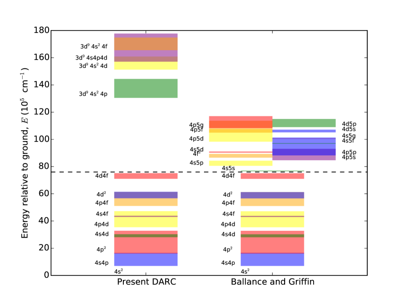
Figure 1: Energy ranges of the configurations included in the present darc calculations and the Ballance and Griffin calculations. Non-relativistic configuration specifications are used for brevity with the understanding they encompass multiple relativistic sub-configurations. The energy ranges are determined by assigning each $jj$-coupled level to the corresponding configuration which contributes the dominant component the level’s state vector. This method can be ambiguous in cases where strong configuration mixing is present.

Additionally, a sample of the radiative data from our grasp⁰ structure results is presented in table 4. Apart from wavelengths, negligible experimental radiative data is available, and so only theoretical results are supplied for comparison. The theoretical results are from the same calculations as in the energy level table 3, excepting the addition of Fournier’s ab initio calculations [12] and the omission of our autostructure results for brevity. The Fournier $gf$ values for the 212–1 and 290–1 transitions are discrepant because the 3d⁹4s4p4d configuration was not included in that calculation, and as demonstrated in section 2.1, the 3d⁹4s4p4d configuration mixes heavily and greatly changes the radiative data of these 3d-subshell transitions. Consequently, comparison of these transitions with calculations that do not include this configuration are not meaningful. Otherwise, the Fournier $gf$ values tend to agree well with our corresponding grasp⁰ results, except for the rather weak transitions 129–6 and 73–10 that differ by about a factor of three.

The Ballance and Griffin grasp⁰ results also appear to be in close agreement with our grasp⁰ results in this sample, except in instances where the magnitude of the $gf$ value is small or the velocity to length ratios are not close to unity. In both cases, this is to be expected when comparing calculations with different CI expansions. A full scope but necessarily more coarse comparison with our results was conducted using scatter plots analogous to those in figure 3. Neither the dipole line strengths, $S_{ik}$, nor the radiative transition probabilities up to quadrupole order revealed any systematic differences between the calculations, and 73% of the values agree within 20% relative error of each other, meaning there is reasonable accord overall. The dipole line strengths are directly proportional to the infinite energy limits of the corresponding EIE collision strength, and so this information will be relevant for the analysis of the collision data in section 3.2.

On the other hand, the Safronova and Safronova results exhibit a binary behaviour: they either agree well with the present results or disagree by a few orders of magnitude. Based on the energy level values quoted by Safronova and Safronova, we can say with a high degree of certainty that this disagreement is not due to a level mismatching by us; however, we did observe significant differences in the wavelength values for these conflicting transitions. Upon further investigation, the wavelengths given by Safronova and Safronova do not agree with their own energy level values. Thus, we suspect that there has been a labelling error in their work. To confirm this hypothesis, we investigated further with autostructure to provide a corroborative third party result. We already had the relevant results from using the CI expansion in section 2.1, and an additional run was conducted using the CI from the Safronova and Safronova work. In both cases, the autostructure results agreed with the present grasp⁰ results, supporting the validity of the present work and pointing to a labelling error in the Safronova and Safronova results.

Table 4: Radiative data: weighted oscillator strength ($gf$) and wavelength ($\lambda$) values for W⁴⁴⁺. GR denotes the present results generated using grasp⁰; F98 denotes the results from Fournier [12]; BG07 denotes the results from Ballance and Griffin [16]; and SS10 denotes the results from Safronova and Safronova [35]. The autostructure results are not presented in the interest of brevity. The level specifications are for the present results, and mapping of levels between the different calculations was determined by matching symmetry ($J\pi$) and energy ($E$), as in the case of the energy level table. Conversion from $A_{ki}$ values to $gf$ values for the BG07 data was necessary for comparision, and we used their calculated energies to do so. For compactness, $\star=$ (3d⁹(²D_5/2)4s_1/2)${}^{\circ}_{2}$4p_3/2. All results are in the length gauge, and $v/l$ denotes the ratio of the velocity gauge to the length gauge. Values presented in the format $\mathrm{X.XXX}\pm\mathrm{YY}$ represent scientific notation in base 10: $\mathrm{X.XXX}\times 10^{\pm\mathrm{YY}}$

.

$i$	$k$	$jj$-coupled CSF of $k$	$J_{i}$	$J_{k}$	$gf_{\textrm{GR}}$	$v/l_{\textrm{GR}}$	$gf_{\textrm{BG07}}$	$v/l_{\textrm{BG07}}$	$gf_{\textrm{F98}}$	$gf_{\textrm{SS10}}$	$\lambda_{\textrm{GR}}$ (Å)
1	295	($\star$)${}^{\circ}_{7/2}$4d5/2 (7/2,5/2)∘	0	1	9.028$-$01	0.89	$-$	$-$	$-$	$-$	5.7330
1	290	3d9(2D3/2)4s24f (3/2,5/2)∘	0	1	1.610$+$00	0.90	$-$	$-$	5.844$+$00	$-$	5.7438
1	275	($\star$)${}^{\circ}_{1/2}$4d3/2 (1/2,3/2)∘	0	1	1.894$+$00	0.91	$-$	$-$	$-$	$-$	5.7917
1	212	($\star$)${}^{\circ}_{3/2}$4d5/2 (3/2,5/2)∘	0	1	3.820$-$01	0.89	$-$	$-$	1.954$+$00	$-$	5.9485
1	208	($\star$)${}^{\circ}_{5/2}$4d3/2 (5/2,3/2)∘	0	1	4.201$-$01	0.91	$-$	$-$	$-$	$-$	5.9616
1	207	($\star$)${}^{\circ}_{3/2}$4d5/2 (3/2,5/2)∘	0	1	4.923$-$01	0.92	$-$	$-$	$-$	$-$	5.9655
1	81	3d9(2D3/2)4s24p (3/2,3/2)∘	0	1	2.912$-$02	0.91	$-$	$-$	2.800$-$02	$-$	6.9483
6	129	3d9(2D3/2)4s24d (3/2,3/2)	1	0	5.017$-$04	0.00	$-$	$-$	1.292$-$03	$-$	6.9367
1	78	3d9(2D5/2)4s24p (5/2,3/2)∘	0	1	2.562$-$01	0.91	$-$	$-$	2.379$-$01	$-$	7.2056
1	75	3d9(2D3/2)4s24p (3/2,1/2)∘	0	1	1.519$-$01	0.91	$-$	$-$	1.412$-$01	$-$	7.3524
4	83	3d9(2D3/2)4s24p (3/2,3/2)∘	2	2	1.580$-$04	0.90	$-$	$-$	1.488$-$04	$-$	7.7453
4	82	3d9(2D3/2)4s24p (3/2,3/2)∘	2	3	1.303$-$04	0.01	$-$	$-$	1.237$-$04	$-$	7.7580
2	74	3d9(2D3/2)4s24p (3/2,1/2)∘	0	2	9.193$-$05	2.20	$-$	$-$	8.710$-$05	$-$	7.7670
3	74	3d9(2D3/2)4s24p (3/2,1/2)∘	1	2	1.301$-$04	8.70	$-$	$-$	1.294$-$04	$-$	7.8015
6	82	3d9(2D3/2)4s24p (3/2,3/2)∘	1	3	1.875$-$04	0.08	$-$	$-$	1.738$-$04	$-$	7.8462
4	79	3d9(2D5/2)4s24p (5/2,3/2)∘	2	3	1.999$-$04	0.01	$-$	$-$	1.839$-$04	$-$	8.0730
4	77	3d9(2D5/2)4s24p (5/2,3/2)∘	2	2	7.144$-$05	0.91	$-$	$-$	6.886$-$05	$-$	8.0880
4	76	3d9(2D5/2)4s24p (5/2,3/2)∘	2	4	4.136$-$04	0.01	$-$	$-$	3.961$-$04	$-$	8.0991
2	72	3d9(2D5/2)4s24p (5/2,1/2)∘	0	2	1.379$-$04	0.88	$-$	$-$	1.313$-$04	$-$	8.0998
3	73	3d9(2D5/2)4s24p (5/2,1/2)∘	1	3	3.229$-$04	0.01	$-$	$-$	2.998$-$04	$-$	8.1327
3	72	3d9(2D5/2)4s24p (5/2,1/2)∘	1	2	8.764$-$05	3.00	$-$	$-$	8.684$-$05	$-$	8.1380
6	77	3d9(2D5/2)4s24p (5/2,3/2)∘	1	2	1.469$-$04	0.04	$-$	$-$	1.494$-$04	$-$	8.1840
11	76	3d9(2D5/2)4s24p (5/2,3/2)∘	3	4	1.940$-$04	2.00	$-$	$-$	3.014$-$04	$-$	9.1878
10	73	3d9(2D5/2)4s24p (5/2,1/2)∘	2	3	3.580$-$05	2.90	$-$	$-$	1.389$-$04	$-$	9.7800
3	12	4s4d (1/2,5/2)	1	2	8.387$-$02	1.00	7.694$-$02	$-$	8.768$-$02	7.500$-$02	44.2929
3	10	4s4d (1/2,3/2)	1	2	1.775$+$00	1.00	1.795$+$00	$-$	1.776$+$00	1.689$+$00	48.2882
1	6	4s4p (1/2,3/2)∘	0	1	1.095$+$00	0.83	1.139$+$00	0.99	1.099$+$00	1.060$+$00	60.6907
3	8	4p2 (1/2,3/2)	1	2	7.290$-$01	0.99	7.460$-$01	$-$	7.256$-$01	$-$	61.6827
6	13	4p2 (3/2,3/2)	1	2	2.351$+$00	1.00	2.393$+$00	$-$	2.404$+$00	2.244$+$00	63.0756
4	12	4s4d (1/2,5/2)	2	2	6.591$-$01	1.00	6.753$-$01	$-$	6.882$-$01	6.350$-$01	66.2383
6	12	4s4d (1/2,5/2)	1	2	4.271$-$01	1.00	4.199$-$01	$-$	3.878$-$01	$-$	73.2493
1	3	4s4p (1/2,1/2)∘	0	1	1.364$-$01	0.59	1.415$-$01	1.00	1.376$-$01	1.320$-$01	132.4223
3	4	4s4p (1/2,3/2)∘	1	2	5.643$-$05	1.00	5.873$-$05	$-$	5.637$-$05	$-$	133.6916
1	16	4p4d (1/2,3/2)∘	0	1	2.185$-$04	1.50	1.484$-$04	0.99	$-$	$-$	27.1909
1	29	4p4d (3/2,5/2)∘	0	1	1.598$-$04	0.95	3.392$-$04	1.10	$-$	$-$	21.3138
1	59	4d4f (3/2,5/2)∘	0	1	3.357$-$05	0.01	4.694$-$05	0.91	$-$	$-$	13.8487
1	71	4d4f (5/2,7/2)∘	0	1	1.885$-$04	0.08	2.402$-$04	1.00	$-$	$-$	13.3697
2	7	4p2 (1/2,3/2)	0	1	5.135$-$01	1.00	5.191$-$01	0.99	$-$	$-$	59.9089
2	9	4s4d (1/2,3/2)	0	1	6.148$-$01	1.00	6.249$-$01	1.00	$-$	$-$	47.6077
2	40	4d2 (3/2,5/2)	0	1	3.898$-$05	0.81	5.350$-$05	0.79	$-$	$-$	19.3960
2	45	4p4f (3/2,5/2)	0	1	6.580$-$05	1.10	9.251$-$05	1.20	$-$	$-$	19.0480
8	19	4s4f (1/2,5/2)∘	2	3	6.398$-$01	1.00	6.714$-$01	$-$	$-$	$-$	52.5430
4	11	4s4d (1/2,5/2)	2	3	1.860$+$00	1.00	1.887$+$00	$-$	$-$	$-$	68.3293
75	129	3d9(2D3/2)4s24d (3/2,3/2)	1	0	2.243$-$01	0.87	$-$	$-$	$-$	$-$	40.5992
20	45	4d2 (3/2,5/2)	2	1	7.047$-$01	0.87	$-$	$-$	$-$	9.000$-$01	60.9793
7	25	4p4d (3/2,3/2)∘	1	1	7.485$-$01	1.00	$-$	$-$	$-$	7.140$-$01	48.2905
8	28	4p4d (3/2,5/2)∘	2	2	5.357$-$03	1.00	$-$	$-$	$-$	8.350$-$01	45.6454
8	26	4p4d (3/2,3/2)∘	2	3	1.071$+$00	1.00	$-$	$-$	$-$	6.550$-$01	47.4473
10	17	4s4f (1/2,5/2)∘	2	3	3.092$-$02	0.97	$-$	$-$	$-$	2.490$+$00	104.8515
17	38	4p4f (3/2,5/2)	3	4	1.973$+$00	1.00	$-$	$-$	$-$	4.389$+$00	49.7191
29	39	4p4f (3/2,7/2)	1	2	4.511$-$02	0.94	$-$	$-$	$-$	1.614$+$00	88.8178

3.2 Collision Data

Moving now to the collision problem, a sample of the data from our darc and autostructure DW calculations is provided in figures 2 and 4, and figure 2 also contains data from the Ballance and Griffin calculations [16] for comparison . This data is provided in the form of collision strengths and effective collision strengths. The dimensionless collision strength, $\Omega(i,j)$, for the transition between atomic states $i$ and $j$, is related to the cross-section, $\sigma(i\rightarrow j)$, by

$$\sigma(i\rightarrow j)=\frac{\pi a_{0}^{2}I_{\mathrm{H}}}{g_{i}k_{i}^{2}}\Omega(i,j)\,,$$ (10)

where $g_{i}$ is the statistical weight of the initial state, $k_{i}$ the wavenumber of the incident electron, $a_{0}$ denotes the Bohr radius and $I_{\mathrm{H}}$ is the ionization potential of the hydrogen atom in the units used for $k_{i}^{2}$.

The effective collision strength, $\Upsilon_{ij}$, is the thermal average of the collision strength, typically a Maxwellian average that is used in the present work:

$$\Upsilon_{ij}=\int^{\infty}_{0}\Omega(i,j)e^{(-\epsilon_{j}/kT_{\mathrm{e}})}\mathrm{d}(\epsilon_{j}/kT_{\mathrm{e}})$$ (11)

where $\epsilon_{j}$ is the final energy of the scattering electron, $T_{\mathrm{e}}$ the electron temperature, and $k$ denotes Boltzmann’s constant. The Maxwell-Boltzmann distribution is non-relativistic, and relativistic effects become significant for $T_{\mathrm{e}}\gtrsim 20$ keV $\approx 2.3\times 10^{8}$ K, relevant to the electron temperatures expected at ITER. In keeping with ADAS convention, we do not apply any relativistic corrections to the electron distribution functions used to produce the $\Upsilon_{ij}$ values in this work. The relativistic Maxwell-Jüttner distribution only requires the application of a simple multiplicative factor to the Maxwell-Boltzmann $\Upsilon_{ij}$ values.

Damping effects are apparent in both the collision strengths and effective collision strengths in figure 2, and our autostructure DW results are always less than the darc results. This should be expected since our DW does not include resonance contributions to the effective collision strengths, which are certainly present for these transitions. However, the high energy behaviour of the DW results does approach that of the darc results as would be expected.

There are obvious differences of the damped effective collision strengths between the present results and the Ballance and Griffin results for transitions 1–2 and 1–24, figures 2(b) and 2(f) respectively. Both of these transitions are non-dipole ($J:0\rightarrow 0$) and comparatively small in magnitude; therefore, damping effects and any differences in the CC expansion tend to be more pronounced. Our lack of a full damping treatment could explain the discrepancies; however, one must first compare the undamped data to resolve the true origin of any differences. Unfortunately, the undamped Ballance and Griffin results are only presented in graphical form in their paper and the original data files are not available [36]. Furthermore, only data for the damped effective collision strengths are available, not the damped collision strengths. A visual comparison with the plots in the Ballance and Griffin paper is still useful. Comparing our undamped effective collision strengths with those of Ballance and Griffin, one still observes large differences: our results are larger by about the same factor as in the damped case. Any differences in the undamped effective collision strengths must be due to differences in the resonant structure of the undamped collision strengths. Indeed, comparing our collision strengths in figures 2(a) and 2(e) with the Ballance and Griffin collision strengths, there are intensity peaks present in our results that are not present in theirs, a direct indication that there are additional intermediate resonances in our CC expansion. For example, transition 1-2 will have the resonance 3d⁹4s²4p$nl$ available in our calculations but not in Ballance and Griffin’s. Combining this and the observation that the relative amount of damping in our results is comparable to the Ballance and Griffin results — inferred again from visual inspection — it is reasonable to conclude that the differences observed here are most likely due to the differences in the CIs and CC expansions and not differences in the treatment of radiation damping. Moreover, discrepancies due to varying resonant enhancement between calculations should be less pronounced in strong dipole allowed transitions, and this is exactly what is observed for the dipole 1-3 transition in figures 2(c) and 2(d).

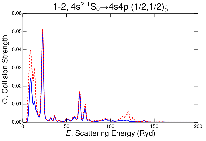
(a)

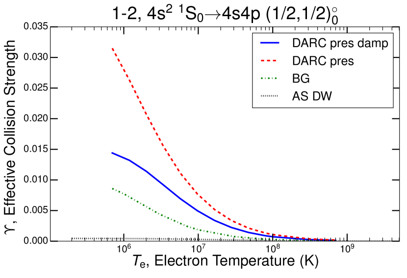
(b)

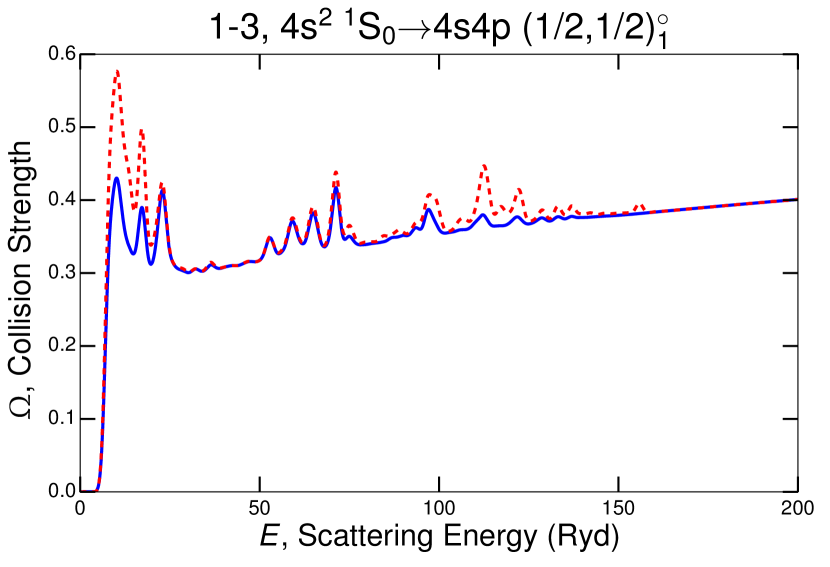
(c)

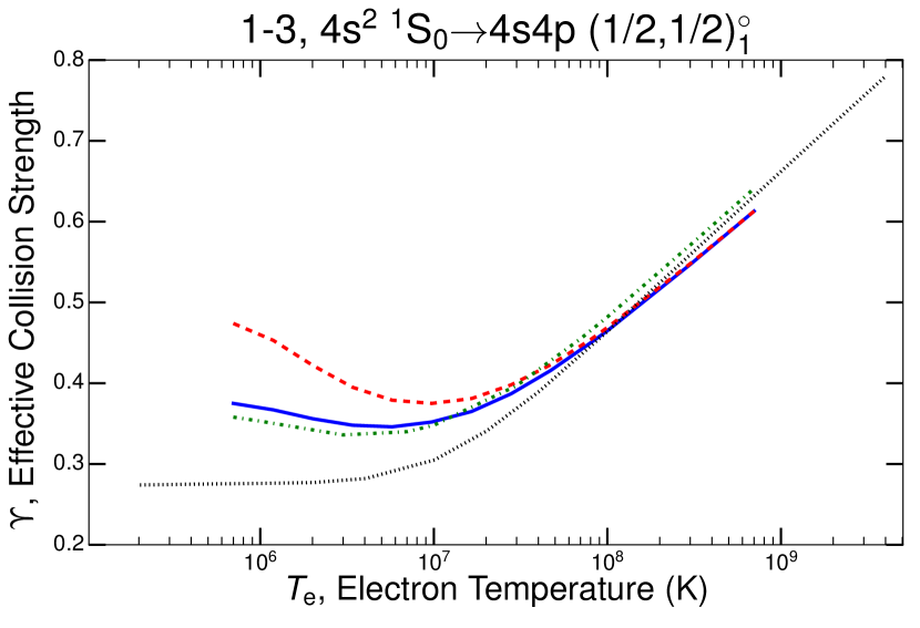
(d)

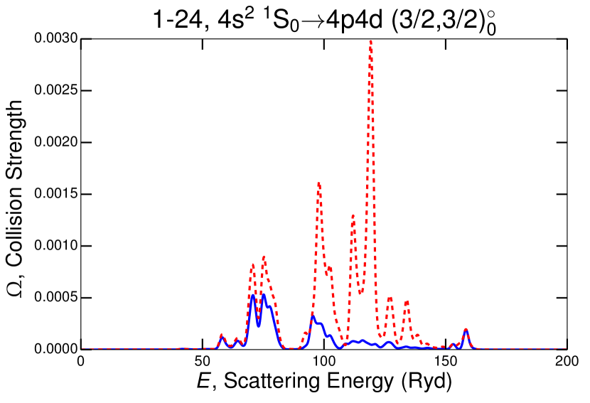
(e)

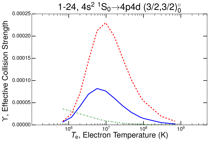
(f)

Figure 2: Collision strength, $\Omega$, and effective collision strength, $\Upsilon$, results for the three transitions presented by Ballance and Griffin in [16]. Figures 2(a), 2(c), and 2(e) display the convolution of the present $\Omega$ data with a 2.205 Ryd (30 eV) Gaussian function; this ‘smoothes’ the dense resonance peaks while still retaining the information about where the peaks are strongest, making interpretation and viewing easier. The dashed (red) line is for the undamped data, and the solid (blue) line for the damped data. Figures 2(b), 2(d), and 2(f) show the present $\Upsilon$ data (DARC pres and DARC pres damp) along with the present autostructure DW (AS DW) results and the corresponding Ballance and Griffin (BG) results [16]. Refer to the legend in 2(b) for the line styles corresponding to each data set.

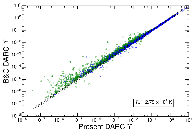
(a)

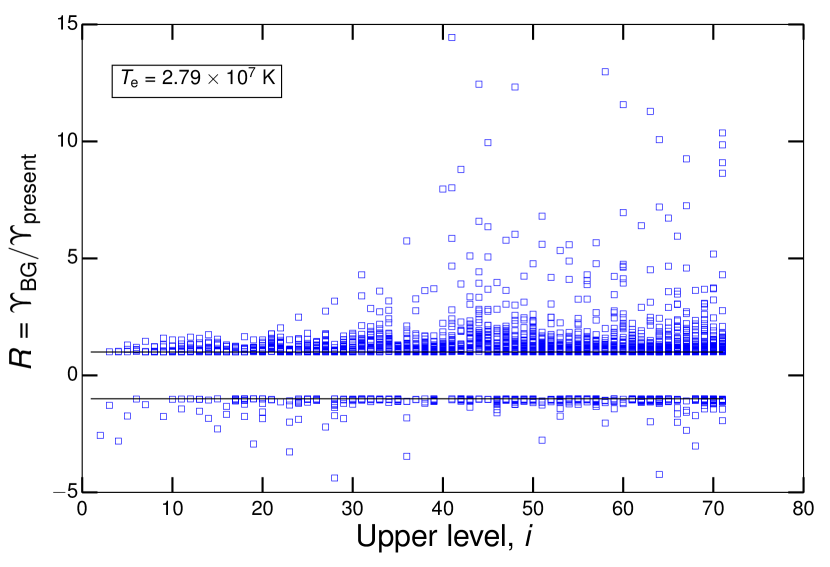
(b)

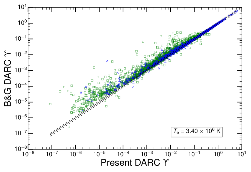
(c)

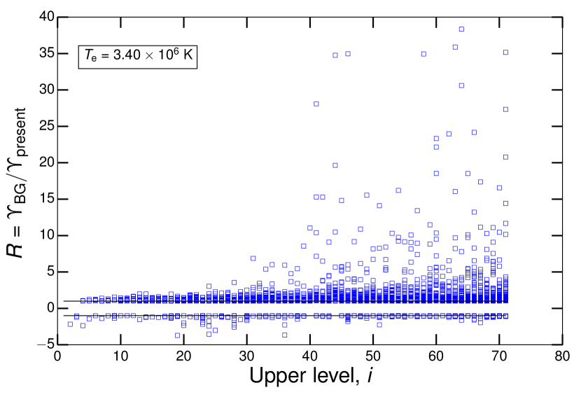
(d)

Figure 3: Comparison — 3(a) and 3(c) — and ratio — 3(b) and 3(d) — scatter plots of effective collision strength values, $\Upsilon$, from the two primary calculations: Ballance and Griffin’s (B&G) fully damped darc versus the present, partially damped darc. The temperature at which the $\Upsilon$ values are being sampled is indicated by the boxed value on each plot. For the comparison plots, 3(a) and 3(c), the (blue) triangles denote dipole transitions, and the (green) squares denote non-dipole transitions. The dotted lines demarcate the 20% error region around the $y=x$ line, and the percentage of points within the error regions are as follows: 3(a) all = 63%, dipole = 82%, non-dipole = 56%; 3(c) all = 44%, dipole = 68%, non-dipole = 35%. For the ratio plots, 3(b) and 3(d), the binary positive or negative behaviour of the ratio is defined by $R=\Upsilon_{\mathrm{BG}}/\Upsilon_{\mathrm{present}}$ if $\Upsilon_{\mathrm{BG}}>\Upsilon_{\mathrm{present}}$ or $R=-\Upsilon_{\mathrm{present}}/\Upsilon_{\mathrm{BG}}$ if $\Upsilon_{\mathrm{BG}}<\Upsilon_{\mathrm{present}}$. The ratio is plotted versus the upper level, $i$, of the transition in each case.

Since these are only two cases, it is not possible to apply this conclusion in general, and it would be impractical to analyze every transition in this manner: there are 2843 intersecting transitions for the two calculations. However, a slightly larger subset of about 15 transitions was analyzed in similar detail, and the same conclusion was reached: our undamped effective collision strengths tend to agree quite well with those of Ballance and Griffin for strong transitions, but weaker transitions display variable levels of agreement. Still, this is not enough evidence to extrapolate our conclusion, so a broader scope technique must be used. Our approach was to select temperatures of interest and then compare the effective collision strength values from the two calculations for all intersecting transitions. Graphically, this results in the comparison scatter plots presented in figures 3(a) and 3(c), one at a temperature near that of peak abundance for W⁴⁴⁺($\approx 3\times 10^{7}$ K) and the other at a lower temperature. The intersecting levels involved in these transitions have an index cut-off of $i=71$, corresponding to the last 3d¹⁰4d4f level. Figure 1 displays that above this configuration, the energy level distributions do not intersect, and therefore there are no overlapping transitions involving levels above this cut-off.

Our limited damping treatment compared to Ballance and Griffin means our collision data should be systematically larger, and this would manifest as a statistically significant number of points lying below the $y=x$ line. However, figures 3(a) and 3(c) display the exact opposite: what appears to be a significant number of points above the $y=x$ lines and so a systematic trend towards our $\Upsilon$ values having comparatively smaller magnitudes. Because the density of points in the vicinity of the $y=x$ line is not readily estimated, it cannot be immediately concluded that this is a statistically significant trend. Calculating the fraction of points within an uncertainty region of 20% around the $y=x$ line can elucidate the situation, and the results of this calculation are presented in the caption of figure 3. The values of 63% and 44% for the all transitions cases indicate that although there is reasonable agreement between most points at these temperatures, a significant portion do lie outside the uncertainty region. Additionally, plotting the ratio of the effective collision strengths, $R=\Upsilon_{\mathrm{BG}}/\Upsilon_{\mathrm{present}}$, versus a relevant independent variable as in figures 3(b) and 3(d) can reveal important systematic trends. Both of these plots show a clear asymmetry of higher $\Upsilon$ values from the Ballance and Griffin calculations. Hence, the significance of the systematic trend is supported.

Since the systematic trend is the opposite to what was expected, there must be another, more significant systematic effect involved other than our limited radiation damping treatment. From the observation of no systematic deviation in the dipole line strengths in section 3.1, it is deduced that the systematic difference cannot be caused directly by differences in the atomic structure. Several indicators suggest that this other systematic effect must be additional resonant enhancement for low to intermediate scattering energies in the Ballance and Griffin calculations. Firstly, the comparison plots in figures 3(a) and 3(c) both show that the trend towards larger $\Upsilon_{\mathrm{BG}}$ values is relatively greater for weaker transitions. The non-dipole transitions, because they tend to be weaker, display a greater susceptibility to the trend, supported by the lower error region percentages and a visibly larger spread of values. Juxtaposing figures 3(a) and 3(c), which only differ by the sampling temperature, reveals that the trend of larger $\Upsilon_{\mathrm{BG}}$ values is enhanced at lower electron temperature, an observation that is also true for figures 3(b) and 3(d). The preceding observations support the claim of additional resonant enhancement because resonances tend to affect weaker, non-dipole transitions to a larger degree and even more so at lower $T_{\mathrm{e}}$.

Secondly, it is seen from the ratio plots in figures 3(b) and 3(d) that the $\Upsilon_{\mathrm{BG}}$ values are increasingly large compared to ours as the index of the upper level, $i$, increases. The upper level is relevant for resonant enhancement considerations because it restricts the possible levels that can be involved in the intermediate ($N+1$) resonant states. As the upper level of a transition approaches the level intersection cut-off of $i=71$ ($E\approx 8\times 10^{6}$ cm^-1 in figure 1), the transition will increasingly only have access to resonances involving levels that are discrepant between the calculations. Consequently, the tendency for $\Upsilon$ values to disagree more at higher $i$ that is observed in figures 3(b) and 3(d) is consistent with the proposition of discordant resonant enhancement.

However, this now begs the question why it is that the Ballance and Griffin results have systematic, additional resonant enhancement, especially when the present calculations include a larger number of levels. The answer must derive from the differing structure of the CC expansions and thus the differing atomic energy level distribution that is summarized in figure 1. The non-intersecting, $n=5$ energy levels in the Ballance and Griffin calculation are immediately above the dashed-line threshold; hence, these levels will be more accessible for resonance formation if the electron distribution functions peaks close to the excitation energy of the transition under consideration. In contrast, the 3d-hole configurations lie $\sim 60$ Ryd higher, as do resonances with the same $n$-value. Furthermore, 3 of these 4 configurations have a strong dipole $4\mathrm{p},4\mathrm{f}\rightarrow 3\mathrm{d}$ type-I radiation damping transition. Finally, some common initial configurations — 4p², 4p4f, 4d², and 4d4f — have no single electron promotions to our 3d-hole resonances, unlike Ballance and Griffin where resonances can be formed by promotion to $n=5$.

One point should be clear from the preceding discussion: it is the composition of the CI and CC expansion that most influences the behaviour of the collision data being compared. Indeed, it is still possible that our calculations neglect a large amount of damping, which would be hidden by the cancellation of the two systematic effects; however, this is unlikely given the analysis of figure 2. The objective of including consideration of the soft x-ray, 3d-subshell transitions had necessarily shaped the CI/CC expansion used in our calculations, and so differences with other calculations should be expected. In the end, a true assessment of the merits of these two primary calculations can only be obtained through the application of the data in the atomic population modelling to follow.

Figure 4 shows the collision data for the strongest three 3d-subshell transitions. Because of the strength of these $E1$ transitions, resonances appear to be unimportant and the behaviour due to direct Coulomb excitation dominates. Such observations are supported by a sharp jump in the collision strengths at the energy threshold of each transition. The limited number of resonance peaks is due to the fact that the upper levels in these transitions are close to the highest energy level included in our calculation, meaning there are comparatively few intermediate resonant states available. Furthermore, good agreement is observed between the autostructure DW results and the darc effective collision strengths. Again, this can be accounted for by the relative sparsity and small magnitude of resonances for these transitions. One might be tempted to conclude that it would be simpler and less time consuming to have only used the DW results; however, it is difficult to predict whether the results will still be similar following atomic population modelling. So it is prudent to carry all available results — present darc, autostructure DW, Cowan PWB, and Ballance and Griffin darc — forward and assess any differences following the final analysis.

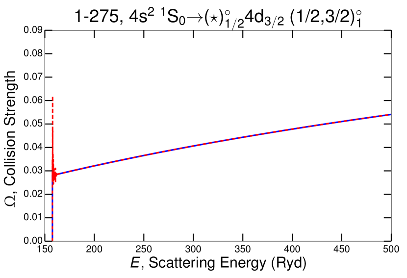
(a)

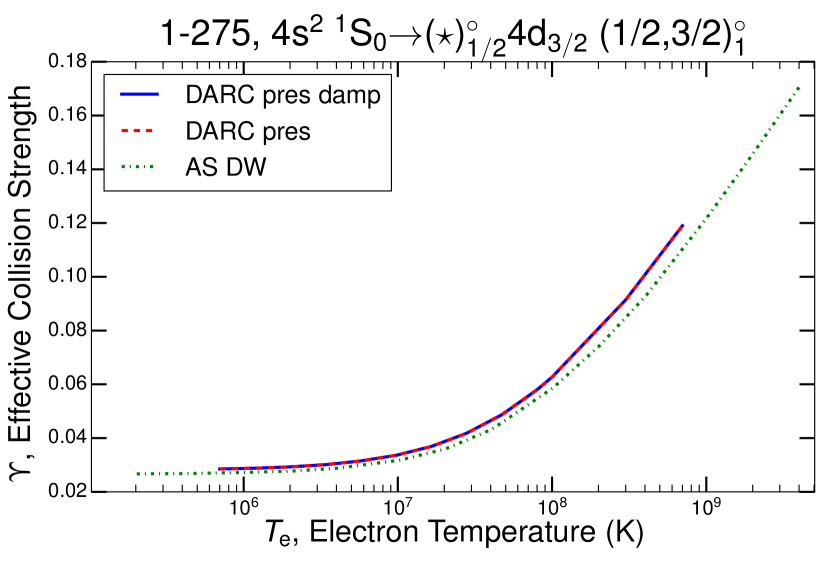
(b)

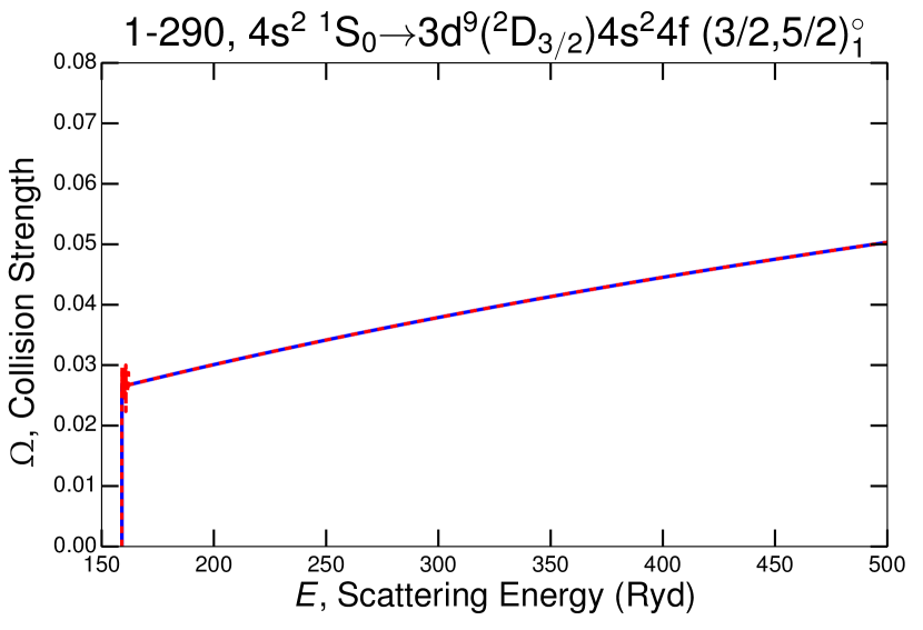
(c)

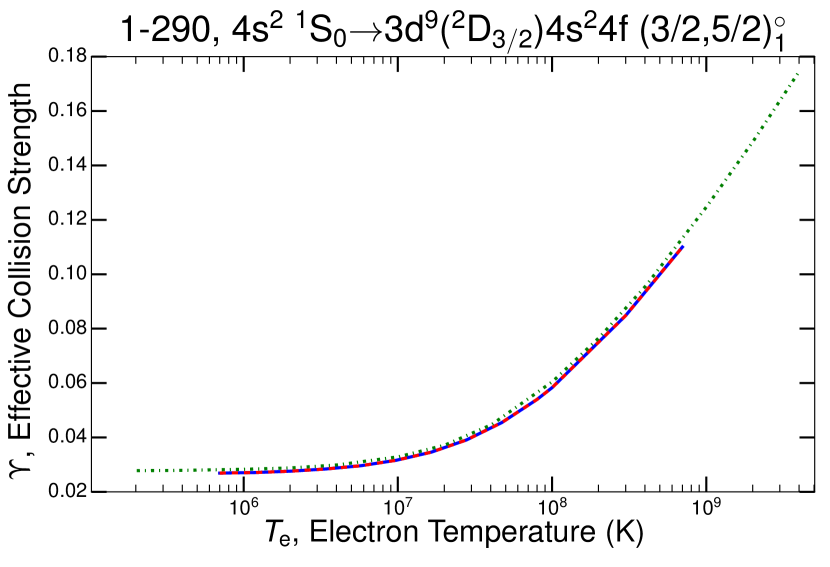
(d)

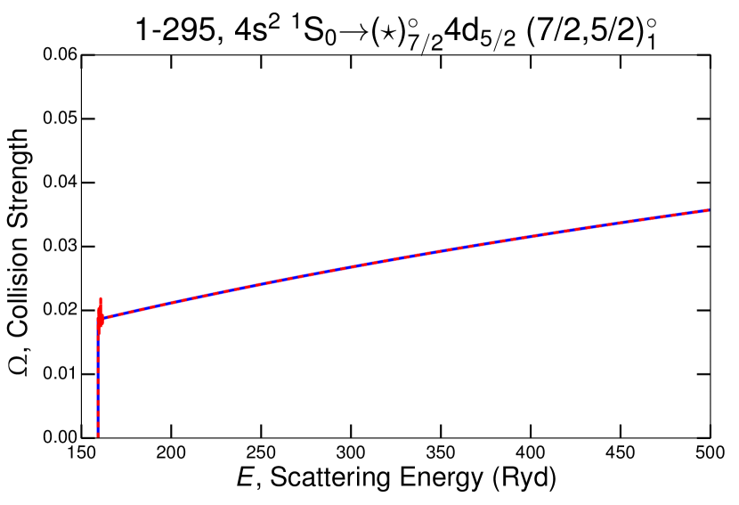
(e)

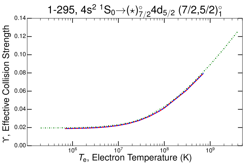
(f)

Figure 4: Present results for the dominant 3d-subshell transitions in the transition arrays, [3d¹⁰4s²–3d⁹4s²4f] and [3d¹⁰4s²–3d⁹4s4p4d]. In contrast to figure 2, 4(a), 4(c), and 4(e) are the ‘raw’ $\Omega$ data sets that have not been convoluted; no convolution is required for these transitions because of the limited resonance structure. Again, the dashed (red) line is for the undamped data, and the solid (blue) line for the damped data. Figures 4(b), 4(d), and 4(f) display the $\Upsilon$ data for both the darc and autostructure DW calculations. Refer to the legend in 4(b) for the corresponding line styles. In the level specifications, the substitution, $\star\equiv$ (3d⁹(²D_5/2)4s_1/2)${}^{\circ}_{2}$4p_3/2, is used.

3.3 Atomic Population Modelling

As noted in Section 1, determination of the total radiated power loss from W⁴⁴⁺ is one of the desirable outputs from atomic population modelling. The excitation line power coefficient for a transition, $j\rightarrow k$, is defined by

$$P_{L,1,j\rightarrow k}=\Delta E_{jk}\mathcal{PEC}^{(\mathrm{exc})}_{1,j\rightarrow k}\ ,$$ (12)

which has units of (W cm³) and is simply the relevant $\mathcal{PEC}$ multiplied by the energy difference between the levels involved, $\Delta E_{jk}$. The total excitation line power coefficient, $P_{LT,1}$, is the sum of the $P_{L,1,j\rightarrow k}$ over all possible transitions and is directly proportional to the total radiated power loss of the ionization stage. Although the $\mathcal{PEC}$s and power coefficients give much of the same information, $\mathcal{PEC}$s are preferred in spectroscopic applications while power coefficients are needed for estimates of radiated power loss. Both are employed in the subsequent analysis and are largely interchangeable in cases where general conclusions about a transition are being sought.

The total excitation line power coefficients from the various calculations are plotted versus electron temperature in figure 5(a), along with a selection of relevant, contributing $P_{L,1,j\rightarrow k}$ from our present darc work. Observing the individual $P_{L,1,j\rightarrow k}$ values, the dominant transition across most of the $T_{\mathrm{e}}$ range is unsurprisingly the dipole allowed 6–1 (60.93 Å); however, towards lower $T_{\mathrm{e}}$ the VUV 3–1 (132.88 Å) transition is stronger due to its lower energy difference. Most importantly for this work, the strongest line from the open 3d-subshell transition arrays is the highlighted 275–1 (5.77 Å) transition. It is the value of the power coefficient at peak abundance temperatures that is of most concern, and a critical observation is that the 275–1 3d-subshell line contributes an equal amount to the total radiated power as does the VUV 3–1 line in this region.

The salient feature of the $P_{LT,1}$ lines in figure 5(a) is the departure of the Ballance and Griffin result from the other calculations at high $T_{\mathrm{e}}$, commencing just before the demarcated region of peak abundance. What causes this behaviour is evident from the individual $P_{L,1,j\rightarrow k}$ lines, just discussed: the 275–1 (5.77 Å) line, which is not included in the Ballance and Griffin calculations, rises to a 50:50 power contribution with the strong VUV 3–1 (132.88 Å) transition in the peak abundance region. Omission of this line along with others of comparable magnitude in the [3d¹⁰4s²–3d⁹4s²4f] and [3d¹⁰4s²–3d⁹4s4p4d] transition arrays leads to the relative reduction in the $P_{LT,1}$ seen in the Ballance and Griffin results. Otherwise, the $P_{LT,1}$ values from the other calculations, both of which include at least some of the important 3d-hole configurations, agree well across the given $T_{\mathrm{e}}$ domain with no relative errors over 50% and convergence at high $T_{\mathrm{e}}$, notably in the shaded region of peak abundance. This reiterates a common theme: the primacy of the configurations included in the collision calculation and subsequent modelling. Without appropriate consideration of the 3d-subshell transitions, a large contribution to the radiated power from W⁴⁴⁺ will be missed, reaffirming our decision to focus attention on these transitions.

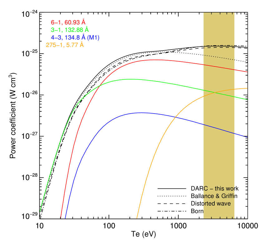
(a)

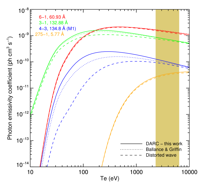
(b)

Figure 5: $P_{LT,1}$, $P_{L,1,j\rightarrow k}$, and $\mathcal{PEC}$ values derived from the relevant fundamental datasets for W⁴⁴⁺ versus electron temperature, $T_{\mathrm{e}}$. The shaded vertical bar represents the $T_{\mathrm{e}}$ range where the fractional abundance of W⁴⁴⁺ in the coronal equilibrium approximation is greater than 0.1. 5(a) shows the total excitation line power coefficients, $P_{LT,1}$, as the enveloping (black) lines, and these have been calculated for the four $\Upsilon$ datasets with line styles indicated in the figure: the Ballance and Griffin darc and the present darc, autostructure DW, and Cowan PWB. A sample of the strongest and most relevant contributing individual lines from the present darc work have been emphasized (coloured) and labelled. 5(b) displays the $\mathcal{PEC}$ lines for the corresponding $P_{L,1,j\rightarrow k}$ lines in 5(a). The line styles denote different datasets as labelled in the figure: Ballance and Griffin’s darc and the present darc and autostructure DW. Note: there are no Ballance and Griffin results for the 275–1 (5.77Å) $\mathcal{PEC}$ line. The indices from our grasp⁰ calculation are used — see tables 3 4.

Figure 5(b) provides a more detailed point of comparison between the calculations by showcasing the $\mathcal{PEC}$s for the same transitions as the individual $P_{L,1,j\rightarrow k}$ lines in figure 5(a). Although the $\mathcal{PEC}$s and $P_{L,1,j\rightarrow k}$ only differ by an energy factor, it is interesting to note the effect that this has upon the importance of the 275–1 (5.77 Å) line; the $P_{L,1,j\rightarrow k}$ values are comparatively higher because of the large energy difference between level 275 and 1. Agreement between the theories in figure 5(b) is quite good for the strong dipole allowed transitions (3–1, 6–1, 275–1), and the moderate discrepancy between the darc and DW results for the 3–1 line can be explained through application of the zero density limit expression in (9). This provides a good approximation in the present circumstance because density effects on level populations are largely absent until $N_{\textrm{e}}\approx 10^{16}$ cm^-3. The dominant $A_{i\rightarrow j}$ value in the sum of (9) is $A_{3\rightarrow 1}$ by many orders of magnitude, and so the $A_{3\rightarrow 1}$ in the numerator will be effectively cancelled. Thus, it must be variation in the excitation rate coefficient, $q_{1\rightarrow 3}^{\mathrm{e}}$, that causes differences in the $\mathcal{PEC}$ values — recall, excitation from the ground dominates in the zero density limit. Indeed, the autostructure DW $\Upsilon_{1\rightarrow 3}$ values are systematically lower than the corresponding darc values because of the absence of resonant enhancement; this explains why the DW $\mathcal{PEC}$ is also lower across the temperature range.

On the other hand, the spin-changing, $M1$, 4–3 transition displays notable differences between all of the calculations, but the $\mathcal{PEC}$ values do eventually converge at high $T_{\mathrm{e}}$. Again, these differences can be understood through the use of the zero density limit for the $\mathcal{PEC}$, and just as above, the contributions from the radiative transition probabilities cancel due to the dominance of the $A_{4\rightarrow 3}$ value. The $\Upsilon_{1\rightarrow 4}$ values for the various calculations reproduce the ordering of the 4–3 $\mathcal{PEC}$ lines in figure 5(b): the autostructure DW $\Upsilon_{1\rightarrow 4}$ are less than both of the darc results because of the absence of resonances, and our darc $\Upsilon_{1\rightarrow 4}$ are larger than Ballance and Griffin’s for less obvious reasons. The trend of relatively larger Ballance and Griffin $\Upsilon$ values observed in section 3.2 in no way means that our $\Upsilon$ values for a particular transition cannot be larger as is the case here; however, the cause of this is indeterminable without the ability to look at the Ballance and Griffin $\Omega$ data.

There are several conclusions relevant to radiated power loss from the observations of figure 5. First, the importance of the soft x-ray 3d-subshell transitions: the $P_{LT,1}$ lines from figure 5(a) clearly show that neglecting the [3d¹⁰4s²–3d⁹4s²4f] and [3d¹⁰4s²–3d⁹4s4p4d] transition arrays will greatly reduce predictions of radiated power loss from W⁴⁴⁺. Thus, these transition arrays must be included in the collision calculations upon which any effort to model radiated power loss is built. Second, there is substantial evidence that the omission of transitions involving the 3d¹⁰4$l$5$l^{\prime}$ configurations (henceforth, $n=5$ transitions) has little effect upon the $P_{LT,1}$ values. The Cowan PWB result, which does include some $n=5$ transitions, does not deviate significantly from the present darc nor the autostructure DW result. Furthermore, Ballance and Griffin collision data for the $n=5$ transitions was merged into our present darc data, and a negligible effect upon the modelled quantities in figure 5 was observed. The $\mathcal{PEC}$s still agreed to within a few percent except for the 4–3, $M1$ transition which agreed within 10%. Even though this merging is not a replacement for a full calculation with all of the relevant configurations, it strongly indicates that the $n=5$ transitions are not essential for radiated power loss considerations in general and therefore also for the 3d-subshell transitions. As discussed in section 3.2, the 3d¹⁰4$l$5$l^{\prime}$ configurations do provide additional resonant enhancement for lower level transitions, and the effect of this in the context of population modelling will require further investigation outside the current scope of the present study.

Thirdly, the overall proximity between the present darc, Cowan PWB, and autostructure DW results in figure 5(a) propounds the suitability of the non-close coupling theories as baseline descriptions of the radiated power from W⁴⁴⁺. However, the precedent statement in no way recommends that the more intensive darc calculations are unnecessary. From a detailed spectroscopic perspective, one must assess the suitability of a particular dataset on a transition-by-transition basis, and the small number of transitions presented in figure 5 do not allow any generalizations to be made. Another technique is required.

Because W⁴⁴⁺ is a heavy and relatively complex species, there are so many transitions that describing it with individual line emissivities is overwhelming and not useful. In response, we produce envelope lines, defined by a vector of feature photon-emissivity coefficients ($\mathcal{F}\textrm{-}\mathcal{PEC}$), that are composite features of many $\mathcal{PEC}$ lines over a wavelength region. Suppose the spectral interval of interest, $[\lambda_{0},\lambda_{1}]$, is partitioned by $N_{p}$ elements of the set, $\left\{\lambda_{i}\equiv\lambda_{0}+i(\lambda_{1}-\lambda_{0})/N_{p}:i=0,\ldots,N_{p}-1\right\}$, then the envelope feature photon emissivity coefficient vector is defined as

$$\mathcal{F}\textrm{-}\mathcal{PEC}{}_{1,i}^{(\textrm{exc})}=\sum_{j,k;\lambda_{j\rightarrow k}\in[\lambda_{0},\lambda_{1}]}\mathcal{PEC}{}_{1,j\rightarrow k}^{(\textrm{exc})}\int_{\lambda_{i}}^{\lambda_{i+1}}\varphi_{j\rightarrow k}(\lambda)\mathrm{d}\lambda$$ (13)

where $\varphi_{j\rightarrow k}(\lambda)$ is the normalized emission profile of the spectrum line $j\rightarrow k$ that defines the line broadening.

The spectral features resulting from the $\mathcal{F}\textrm{-}\mathcal{PEC}$ vectors of the various W⁴⁴⁺ datasets are plotted in figure 6; portions of soft x-ray and VUV regions are represented. As might be expected, the intensities of the features which envelop strong transition lines agree well — the peaks labelled by 6–1 & 8–3 ($\sim 61$ Å) and 3–1 & 4–3 ($\sim 132$ Å). However, the 6–1 feature does display some wavelength discrepancy. The Cowan PWB result overestimates slightly compared to the two darc results. For features of less intense lines, the disagreements are larger: the Cowan PWB result differs from the two darc results by nearly an order of magnitude for both the 12–4 & 11–4 ($\sim 66$ Å) and 12–6 ($\sim 73$ Å) features. Additionally, the 10–3 & 9–2 ($\sim 48$ Å) peak exhibits both intensity and wavelength discrepancies between all the calculations. Overall, figure 6 also clarifies the wavlength coverage of these three datasets. Of most relevance for this work is that there is no Ballance and Griffin result for the 275–1 & 290–1 ($\sim 7$ Å) feature, which is the third most intense. Again, this corresponds to the dominant soft x-ray, 3d-subshell transitions that we have been concerned with throughout, and our darc result is in close agreement with the Cowan PWB. In addition, our darc work has no data between 10 Å and 20 Å corresponding to where the $n=5\textrm{--}4$ lines lie.

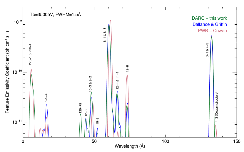
Figure 6: The envelope feature photon-emissivity coefficient, $\mathcal{F}\textrm{-}\mathcal{PEC}$, vectors for various W⁴⁴⁺ calculations plotted versus wavelength at $T_{\mathrm{e}}=T_{\mathrm{i}}=3.5$ keV, where $T_{\mathrm{i}}$ is the ion temperature. The calculations shown are those indicated in the top right, colour-coded legend: Ballance and Griffin’s darc, and the present darc and PWB based on Cowan’s code. The Doppler broadening by the velocity distribution of the radiating ions has been applied using the default Maxwellian distribution with $T_{\mathrm{i}}=T_{\mathrm{e}}$. In addition, the results were convolved with an ideal spectrometer instrument function with a FWHM of 1.5 Å. The vertical labelling of the peaks denotes the transition(s) for the dominant excitation $\mathcal{PEC}$(s) within the feature; the indices from our grasp⁰ calculation are used — see tables 3 4.

The unifying message from the observations of figure 6 is that there are enough differences between the CC and non-CC calculations such that applications in detailed spectroscopy could produce disparate results — for example, when calculating the line emissivity, $\varepsilon_{i\rightarrow k}$, from (2). However, the two darc results do agree very well for overlapping spectral intervals. This further supports the conclusion above that our neglect of the $n=5$ transitions has not significantly affected the modelled results. A possible criticism of this conclusion is that only strong emission lines are being considered in figure 6 and that differences between the datasets might become more apparent for weaker lines. But this point is moot: the very fact that these lines are weak and not part of this spectrum means they will not be observable and so are irrelevant from an experimental standpoint. Therefore, for both spectroscopic and radiated power applications, we recommend our darc adf04 file with the merged $n=5$ transition data from Ballance and Griffin.

4 Conclusion

Fully relativistic, partially radiation damped, Dirac $R$-matrix calculations for the EIE of W⁴⁴⁺ have been carried-out using the grasp⁰/darc suite. The energy levels, radiative rates, and effective collision strengths from the present work are available in the adf04 file format on the OPEN-ADAS website: http://open.adas.ac.uk/detail/adf04/znlike/znlike_mmb15][w44ic.dat. The primary objective and motivation for these calculations was to incorporate both of the spectroscopically important transition arrays, [3d¹⁰4s²–3d⁹4s²4f] and [3d¹⁰4s²–3d⁹4s4p4d], which, to the best of our knowledge, had not been done until now. Ultimately, any evaluation of our calculations must be made while keeping this objective in mind. In addition, our autostructure BPDW and Cowan PWB calculations were conducted concurrently to provide baseline comparisons.

The inclusion of the configurations associated with the 3d-subshell transitions required compromises to be made in the CI/CC expansion; configurations 3d¹⁰4$lnl^{\prime}$ for $n>4$ were excluded due to computational limits. Conversely, the Ballance and Griffin Dirac $R$-matrix calculations with which we compare included configurations for $n=5$ but did not open the 3d-subshell to accommodate the 3d-subshell transitions. This difference in the CI/CC expansions leads to a systematic difference between the $\Upsilon$ datasets which is likely caused by an increase in resonant enhancement of the Ballance and Griffin results, rather than being due to target structure or radiation damping variation.

Inevitably, evaluation of the differences in fundamental collision data is performed through its application in atomic population modelling. From the perspective of radiated power loss, it is clear from the $P_{LT,1}$ and $P_{L,1,j\rightarrow k}$ lines that the effect of the 3d-subshell transitions is far greater than any effects due to the neglect of the $n=5$ transitions. Moreover, the non-CC calculations provide a suitable baseline for radiated power loss estimates. Spectroscopically, differences in the $\mathcal{F}\textrm{-}\mathcal{PEC}$ spectra demonstrate that the $R$-matrix (CC) calculations are necessary for detailed applications, but the close agreement of our darc results with those of Ballance and Griffin further supports the conclusion that omitting the $n=5$ transitions does not have a large effect upon the modelled results. Indeed, it is the inclusion of the 3d-subshell transitions, which create a relatively strong spectral feature, that is of greater import. In the future, it would be advantageous to extend the present calculations to include the 3d¹⁰4$l$5$l^{\prime}$ configurations so as to unequivocally resolve the effect of the additional resonant enhancement upon the lower lying transitions in the context of atomic population modelling.

References

- [1] Bolt H, Barabash V, Krauss W, Linke J, Neu R et al. 2004 J. Nucl. Mater. 329-333 66–73
- [2] Federici G, Skinner C H, and Brooks J N 2001 Nucl. Fusion 41(12) 1967
- [3] Pitts R A, Carpentier S, Escourbiac F, Hirai T, Komarov V et al. 2013 J. Nucl. Mater. 438 S48–S56
- [4] Aymar R 2001 Summary of the ITER Final Design Report, ITER Doc. G A0 FDR Technical report ITER URL http://www-pub.iaea.org/MTCD/publications/PDF/ITER-EDA-DS-22.pdf
- [5] Aymar R, Barabaschi P, and Shimomura Y 2002 Plasma Phys. Control. Fusion 44(5) 519–565
- [6] ITER Physics Expert Group on Divertors, ITER Physics Expert Group on Divertor Modelling and Database, and ITER Physics Basis Editors 1999 Nucl. Fusion 39(12) 2391–2469
- [7] Shumack A E, Rzadkiewicz J, Chernyshova M, Jakubowska K, Scholz M et al. 2014 Rev. Sci. Instrum. 85 11E425
- [8] Kramida A E and Shirai T 2009 At. Data Nucl. Data Tables 95(3) 305–474
- [9] Kramida A E 2011 Can. J. Phys. 89(5) 551–570
- [10] Clementson J, Beiersdorfer P, Brown G V, and Gu M F 2010 Phys. Scr. 81 015301
- [11] Neill P, Harris C, Safronova A S, Hamasha S, Hansen S et al. 2004 Can. J. Phys. 82(11) 931–942
- [12] Fournier K B 1998 At. Data Nucl. Data Tables 68(1) 1–48
- [13] Spencer S, Hibbert A, and Ramsbottom C A 2014 J. Phys. B 47 245001
- [14] Pütterich T, Neu R, Dux R, Whiteford A D, O’Mullane M G et al. 2008 Plasma Physics and Controlled Fusion 50(8) 085016
- [15] Robicheaux F, Gorczyca T W, Pindzola M S, and Badnell N R 1995 Phys. Rev. A 52(2) 1319–1333
- [16] Ballance C P and Griffin D C 2007 J. Phys. B 40(2) 247–258
- [17] Das T, Sharma L, and Srivastava R 2012 Phys. Scr. 86(3) 035301
- [18] Summers H P 2007 Atomic Data and Analysis Structure User Manual URL http://www.adas.ac.uk
- [19] Badnell N R 1986 J. Phys. B: At. Mol. Phys. 19 3827–3835
- [20] Badnell N R 1997 J. Phys. B 30(1) 1–11
- [21] Badnell N R 2011 Comput. Phys. Commun. 182(7) 1528–1535
- [22] Grant I P, McKenzie B J, Norrington P H, Mayers D F, and Pyper N C 1980 Comput. Phys. Commun. 21(2) 207–231
- [23] McKenzie B J, Grant I P, and Norrington P H 1980 Comput. Phys. Commun. 21(2) 233–246
- [24] Dyall K G, Grant I, Johnson C T, Parpia F A, and Plummer E P 1989 Comput. Phys. Commun. 55(3) 425–456
- [25] Norrington P 2009 “GRASP0 and DARC Repository” URL http://web.am.qub.ac.uk/DARC/
- [26] Badnell N R, Foster A, Griffin D C, Kilbane D, O’Mullane M et al. 2011 J. Phys. B 44 135201
- [27] Bauche J and Bauche-Arnoult C 1987 J. Phys. B: At. Mol. Phys. 20 1443–1450
- [28] Cowan R D 1981 The Theory of Atomic Structure and Spectra University of California Press
- [29] Mitnik D M, Griffin D C, and Badnell N R 2001 J. Phys. B: At. Mol. Opt. Phys. 34(22) 4455
- [30] Mitnik D M, Griffin D C, Ballance C P, and Badnell N R 2003 J. Phys. B: At. Mol. Opt. Phys. 36 717
- [31] Ballance C P and Griffin D C 2004 J. Phys. B 37(14) 2943–2957
- [32] Ballance C P and Griffin D C 2006 J. Phys. B 39(17) 3617–3628
- [33] Seaton M J 1983 Rep. Prog. Phys. 167(2) 167
- [34] Burgess A and Tully J A 1992 Astron. Astrophys. 254 436–453
- [35] Safronova U I and Safronova A S 2010 J. Phys. B: At. Mol. Opt. Phys. 43(7) 074026
- [36] Ballance C P “Private Communication, 2014”