Magnetic field growth in young glitching pulsars with a braking index

Abstract

In the standard scenario for spin evolution of isolated neutron stars, a young pulsar slows down with a surface magnetic field $B$ that does not change. Thus the pulsar follows a constant $B$ trajectory in the phase space of spin period and spin period time derivative. Such an evolution predicts a braking index $n=3$ while the field is constant and $n>3$ when the field decays. This contrasts with all nine observed values being $n<3$. Here we consider a magnetic field that is buried soon after birth and diffuses to the surface. We use a model of a growing surface magnetic field to fit observations of the three pulsars with lowest $n$: PSR J0537$-$6910 with $n=-1.5$, PSR B0833$-$45 (Vela) with $n=1.4$, and PSR J1734$-$3333 with $n=0.9$. By matching the age of each pulsar, we determine their magnetic field and spin period at birth and confirm the magnetar-strength field of PSR J1734$-$3333. Our results indicate that all three pulsars formed in a similar way to central compact objects (CCOs), with differences due to the amount of accreted mass. We suggest that magnetic field emergence may play a role in the distinctive glitch behaviour of low braking index pulsars, and we propose glitch behaviour and characteristic age as possible criteria in searches for CCO descendants.

1 Introduction

The magnetic field strength on the surface of neutron stars (NSs) spans a wide range: from $B\sim 10^{8}-10^{9}\mbox{ G}$ for millisecond pulsars and NSs in low-mass X-ray binaries, through $10^{12}-10^{13}\mbox{ G}$ for normal radio pulsars, to $10^{14}-10^{15}\mbox{ G}$ for magnetars. The primary method used to determine these magnetic fields is by measuring each pulsar’s spin period $P$ and spin period time derivative $\dot{P}$. Then assuming that the pulsar rotational energy decreases as a result of emission of magnetic dipole radiation, the surface field strength $B$ at the magnetic pole is inferred, i.e.,

$$P\dot{P}=\frac{\gamma}{2}B^{2}\quad\Leftrightarrow\quad B=6.4\times 10^{19}\mbox{ G }(P\dot{P})^{1/2},$$ (1)

where $\gamma=4\pi^{2}R^{6}\sin^{2}\alpha/3c^{3}I=4.884\times 10^{-40}\mbox{ s G${}^{-2}$ }R_{6}^{6}I_{45}^{-1}\sin^{2}\alpha$, $R$ and $I$ are the NS radius and moment of inertia, respectively, $\alpha$ is the angle between the stellar rotation and magnetic axes, and $R_{6}=R/10^{6}\mbox{ cm}$ and $I_{45}=I/10^{45}\mbox{ g cm${}^{2}$}$ (Gunn & Ostriker 1969; see also Spitkovsky 2006; Contopoulos et al. 2014). Figure 1 shows the measured pulsar spin period and spin period derivative values taken from the ATNF Pulsar Catalogue (Manchester et al., 2005). Also shown is a set of parallel lines which indicates the inferred magnetic field obtained from eq. (1). The other set of parallel lines indicates the pulsar spin-down or characteristic age $\tau_{\rm c}=P/2\dot{P}$; $\tau_{\rm c}$ is often used as a surrogate for the true age of a pulsar.

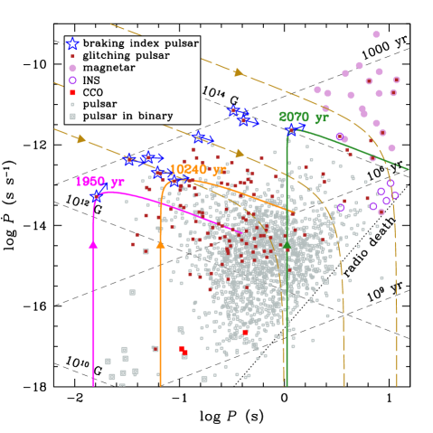
Figure 1: Pulsar spin period $P$ versus spin period time derivative $\dot{P}$. Open squares denote pulsars whose values are taken from the ATNF Pulsar Catalogue; pulsars in a binary system and pulsars that have been observed to glitch are also noted. The nine stars denote pulsars with a measured braking index (see Table 1), with arrows indicating the direction each pulsar is evolving, as determined by their braking index. Closed and open circles and closed squares denote magnetars and isolated neutron stars (INSs) and central compact objects (CCOs), respectively. Short-dashed lines indicate characteristic age $\tau_{\rm c}$ ($=P/2\dot{P}$) and inferred magnetic field $B$ [$=6.4\times 10^{19}\mbox{ G }(P\dot{P})^{1/2}$]. Dotted line indicates the (theoretically uncertain) death line for pulsar radio emission. Solid lines indicate evolution trajectories (to age = $10^{6}\mbox{ yr}$) where the magnetic field is buried initially and (from left to right) the initial field strength and spin period and burial density are [$B_{0}$(G),$P_{0}$(s),$\log\rho_{\rm b}(\mbox{g cm${}^{-3}$})$] = ($3.4\times 10^{12}$,0.015,11.0), ($1.1\times 10^{13}$,0.066,11.5), and ($1.3\times 10^{14}$,1.06,10.5), respectively. Long-dashed lines indicate trajectories where the magnetic field evolves according to eq. (3) and (from left to right) the initial field strength and field decay timescale are [$B_{0}$(G),$\tau$(yr)] = ($8\times 10^{12}$,$10^{6}$), ($3\times 10^{13}$,$10^{6}$), and ($3\times 10^{14}$,$10^{5}$), respectively.

The standard scenario for the rotational evolution of a pulsar is that it is born rapidly spinning (e.g., with an initial spin period $P_{0}$ in the millisecond regime) and rapidly slowing or spinning down, i.e., large $\dot{P}$. This would place a newborn pulsar in the top-left region of Fig. 1. As it spins down, the pulsar moves for $\sim 10^{5}-10^{6}\mbox{ yr}$ along a $P$–$\dot{P}$ path that tracks one of the short-dashed lines of constant magnetic field, evolving towards the bottom-right. This is because magnetic field diffusion and decay occurs on the Ohmic timescale

$$\tau_{\mathrm{Ohm}}=\frac{4\pi\sigma_{\rm c}L^{2}}{c^{2}}\sim 4\times 10^{5}\mbox{ yr}\left(\frac{\sigma_{\rm c}}{10^{23}\mbox{ s${}^{-1}$}}\right)\left(\frac{L}{1\mbox{ km}}\right)^{2},$$ (2)

where $\sigma_{\rm c}$ is the electrical conductivity, $L$ is the lengthscale over which decay occurs, and 1 km is the approximate size of the stellar crust (see Fig. 2); note that magnetic field changes can occur earlier for magnetars due to Hall effects which operate on a timescale $\tau_{\mathrm{Hall}}=(4\pi en_{\rm e}L^{2})/(cB)\sim 2\times 10^{5}\mbox{ yr}\,(\rho/10^{12}\mbox{ g cm${}^{-3}$})(B/10^{14}\mbox{ G})^{-1}(L/1\mbox{ km})^{2}$, where $e$ is electron charge, $n_{\rm e}$ is electron number density, and $\rho$ is mass density (Goldreich & Reisenegger, 1992) (see also Glampedakis et al. 2011). In this work, we are primarily concerned with normal pulsars with $B\sim 10^{12}-10^{13}\mbox{ G}$ and ages $<\mbox{a few}\times 10^{4}\mbox{ yr}$. Thus at times $t\ll\tau_{\mathrm{Ohm}}$, the magnetic field does not change, and $\tau_{\rm c}$ may be an adequate estimate of pulsar age (see Section 4). However when $t\rightarrow\tau_{\mathrm{Ohm}}$, the magnetic field decreases, causing the efficiency of dipole radiation to decrease and $\dot{P}\rightarrow 0$ [see eq. (1)]. Simple examples of such evolutionary paths are shown by the long-dashed curves in Fig. 1, for different initial magnetic field $B_{0}$ and decay timescale. In particular, we assume a magnetic field that evolves with time as

$$B(t)=\frac{B_{0}}{1+t/\tau},$$ (3)

where $\tau$ is the field decay timescale which can be taken to be approximately equal to $\tau_{\mathrm{Ohm}}$ (or $\tau_{\mathrm{Hall}}$ for magnetars). Equation (3) mimics the results of numerical simulations of magnetic field evolution in the crust (see, e.g., Colpi et al. 2000). Observations and theoretical work seem to support the above scenario of an approximately constant magnetic field early in the life of a pulsar and a slowly decaying field at later times (e.g., Viganò et al. 2013 find that the magnetic field is constant until an age of $\mbox{a few}\times 10^{6}\mbox{ yr}$ for $B_{0}\lesssim 10^{14}\mbox{ G}$ and $\sim 10^{5}\mbox{ yr}$ for $B_{0}\gtrsim 10^{14}\mbox{ G}$, and Igoshev & Popov 2014 find a field decay timescale of $\sim 4\times 10^{5}\mbox{ yr}$).

On the other hand, there also exist observations that suggest that the magnetic field evolves, and especially fields that grow, in young NSs. An important example comes from the (measured) braking index of pulsars. The second time derivative of the period $\ddot{P}$ can be determined in a few pulsars (where $\ddot{P}$ is not dominated by timing noise), and $\ddot{P}$ is conventionally expressed in terms of the braking index $n$, which is given by

$$n=2-\frac{P\ddot{P}}{\dot{P}^{2}}.$$ (4)

If pulsar spin-down is due to only magnetic dipole radiation and the field is constant, then eq. (1) yields a braking index $n=3$. However, $n<3$ for all pulsars with a measured $\ddot{P}$ (see Table 1). The low observed values of $n$ can be attributed to a magnetic field that is increasing: allowing $B$ to evolve in eq. (1), one easily obtains

$$n=3-2\frac{\dot{B}}{B}\frac{P}{\dot{P}}=3-4\tau_{\rm c}\frac{\dot{B}}{B}=3-\frac{4}{\gamma}\frac{\dot{B}}{B^{3}}P^{2},$$ (5)

where $\dot{B}$ is time derivative of $B$. For each pulsar with a measured braking index, we denote its possibly evolving field in Fig. 1 by arrows directed along a pulsar’s trajectory in $P$–$\dot{P}$ phase space (see also Espinoza et al. 2011b; Espinoza 2013). It is clear that about five of the nine pulsars are moving along trajectories almost parallel to (short-dashed) lines of constant $B$, and these are pulsars with braking index between 2 and 3. Two pulsars (PSR J0537$-$6910 and J1734$-$3333) are clearly crossing lines of constant $B$, thus suggesting that their fields are growing and J1734$-$3333 is evolving into a magnetar (Espinoza et al., 2011b). Note that we assume a constant $\alpha$ for simplicity [see eq. (1)]. An evolving $\alpha$ can produce similar spin evolution behaviour to one with $\dot{B}$. However evidence for a varying $\alpha$ is uncertain (see, e.g., Lyne et al. 2013, 2015), and for example, Guillón et al. (2014) find that either $\alpha$ is constant or the timescale for its variation is very long.

Table 1: Pulsars with a measured braking index $n$. Spin periods $P$ and period derivatives $\dot{P}$ are taken from the ATNF Pulsar Catalogue. Number in parentheses is uncertainty in last digit of braking index. Glitch data are taken from the Glitch Catalogue and from Ho et al. (2015), and references therein. References for age and braking index: [1] Lyne et al. 1993, [2] Wang & Gotthelf 1998; Chen et al. 2006, [3] Middleditch et al. 2006, [4] Park et al. 2010, [5] Gradari et al. 2011, [6] Page et al. 2009; Tsuruta et al. 2009, [7] Lyne et al. 1996, [8] Kumar et al. 2012, [9] Weltevrede et al. 2011, [10] Gaensler et al. 1999, [11] Livingstone & Kaspi 2011, [12] Ho & Andersson 2012, [13] Espinoza et al. 2011b, [14] Bocchino et al. 2005; Camilo et al. 2006, [15] Roy et al. 2012, [16] Blanton & Helfand 1996, [17] Livingstone et al. 2007, 2011.

Pulsar	SNR	$P$	$\dot{P}$	$\tau_{\rm c}$	Age	Braking	No. of	Typical
		(s)	(s s-1)	(yr)	(yr)	index $n$	glitches	$\Delta\Omega/\Omega$
B0531$+$21	Crab	0.0331	4.23$\times 10^{-13}$	1240	961	2.51(1) [1]	25	$10^{-9}-10^{-8}$
J0537$-$6910	N157B	0.0161	5.18$\times 10^{-14}$	4930	2000${}^{+3000}_{-1000}$ [2]	$-1.5$(1) [3]	45	$10^{-7}$
B0540$-$69	0540$-$69.3	0.0505	4.79$\times 10^{-13}$	1670	1000${}^{+660}_{-240}$ [4]	2.087(7) [5]	1	$10^{-9}$
B0833$-$45	Vela	0.0893	1.25$\times 10^{-13}$	11300	11000${}^{+5000}_{-5600}$ [6]	1.4(2) [7]	19	$10^{-6}$
J1119$-$6127	G292.2$-$0.5	0.408	4.02$\times 10^{-12}$	1610	7100${}^{+500}_{-2900}$ [8]	2.684(2) [9]	3	$10^{-9}-10^{-6}$
B1509$-$58	G320.4$-$1.2	0.151	1.53$\times 10^{-12}$	1570	$<21000$ [10]	2.832(3) [11]	0	—
J1734$-$3333	G354.8$-$0.8	1.17	2.28$\times 10^{-12}$	8130	$>1300$ [12]	0.9(2) [13]	1	$10^{-7}$
J1833$-$1034	G21.5$-$0.9	0.0619	2.02$\times 10^{-13}$	4850	1000${}^{+200}_{-800}$ [14]	1.8569(6) [15]	4	$10^{-9}$
J1846$-$0258	Kesteven 75	0.327	7.11$\times 10^{-12}$	728	1000${}^{+3300}_{-100}$ [16]	2.65(1) [17]	2	$10^{-9}-10^{-6}$

In this work, we describe an alternative to the standard scenario for pulsar spin evolution described above, one that provides a physical mechanism for a growing magnetic field, using the model of Ho (2011) (see also Muslimov & Page 1996; Geppert et al. 1999; Viganò & Pons 2012). In brief, pulsars are born with a strong field, but this field was buried by an early episode of accretion and is slowly diffusing to the surface. In such cases, the surface field responsible for spin evolution [including $n<3$ from eq. (5)] is increasing at the current epoch. Since glitches and timing noise could be responsible for small changes in $n$ (see Livingstone et al. 2011; Antonopoulou et al. 2015; Lyne et al. 2015), we only consider pulsars with a braking index less than half that predicted by the standard scenario (i.e., $n<1.5$) as sources whose braking index requires an explanation beyond the standard scenario (see Espinoza et al. 2011b; Lyne et al. 2015, and references therein, for discussion of other models for low braking index; see also Hamil et al. 2015). From Table 1 we see that this criterion is satisfied by three pulsars: PSR J0537$-$6910, B0833$-$45 (Vela), and J1734$-$3333; note that Muslimov & Page (1996) considered B0531$+$21 (Crab), B0540$-$69, and B1509$-$58 which have $n>2.1$. In Section 2, we briefly describe the model for magnetic field evolution. In Section 3, we present our results and use the measured braking index and age of the three pulsars to determine the initial magnetic field and spin period of each pulsar and the amount of matter each accreted. In Section 4, we summarize our findings and discuss their implications.

2 Magnetic field evolution model

Our calculation of magnetic field evolution follows that of Urpin & Muslimov (1992) and Ho (2011). Here we provide a summary and describe updates (see Ho 2011, for details). The magnetic field is assumed to be buried deep beneath the surface by a post-supernova episode of hypercritical accretion (Chevalier, 1989; Geppert et al., 1999; Bernal et al., 2010, 2013). The field then diffuses to the surface on a timescale that depends on burial depth. One might expect an anti-correlation between field growth rate and pulsar velocity since a smaller amount of mass will be accreted if the pulsar is moving at a greater velocity; observations tentatively support such a relation (Güneydaş & Ekşi, 2013).

To determine the evolution of the buried magnetic field, we solve the induction equation

$$\frac{\partial{\mathbf{B}}}{\partial t}=-\nabla\times\left(\frac{c^{2}}{4\pi\sigma_{\rm c}}\nabla\times{\mathbf{B}}\right).$$ (6)

Our interest is in the NS crust, which is predominantly in a solid state, and thus we neglect internal fluid motion. We take the surface field after NS formation, but prior to mass accretion, as the magnetic field strength at birth $B_{0}$. Accretion then buries and compresses this birth field. We assume a dipolar field in the stellar interior. In Ho (2011), we consider two field configurations: one in which the field is confined in the crust and another in which the field extends into the core. In the crust-confined case, the surface field grows at first but then decays at later times. In the crust-core field case, the surface field strength grows until it saturates at the level of the core field, and the core field decays on a much longer timescale ($>10^{6}\mbox{ yr}$, especially if the core is superconducting). Results for these two cases are qualitatively similar during the epoch of field growth. Here we consider only the latter case and hold the core field strength constant (see Luo et al. 2015, for more results with a crust-confined field). A constant core field is justified since the Ohmic decay timescale [see eq. (2)] in the core is longer than our times of interest ($t\ll 10^{6}\mbox{ yr}$).

We updated the magnetic field evolution code used in Ho (2011) in primarily two ways. First, we use NS crust and core models built with the APR (Akmal et al., 1998), BSk20, or BSk21 (Potekhin et al., 2013) models of the nuclear equation of state (EOS). In the top panel of Fig. 2, we show the mass above a given density $\Delta M$ [$\equiv M-m(r)$, where $M$ is total NS mass and $m(r)$ is mass enclosed within radius $r$]. $\Delta M$ is an indication of the amount of accreted mass needed to bury the magnetic field to a given density. The bottom panel shows the crust depth ($\equiv R-r$) as a function of density for different NS masses and EOSs. While $\Delta M(\rho)$ is weakly dependent on total NS mass and EOS, depth versus density is a strong function of $M$ and EOS. For a given EOS model (e.g., APR), crust thickness decreases with increasing mass. Therefore to bury the magnetic field at a particular density, the field must be buried at a greater depth for a lower $M$. For different EOS models, we see that the result for BSk20 is very similar to that for APR, and thus the field evolution timescale [which scales with depth, or $L$, as given by eq. (2) for the Ohmic timescale] for BSk20 and APR will be comparable. Depth at a given density for NSs built using BSk21 is larger than that for NSs built using APR, and thus the field evolution timescale for BSk21 will be longer than that for APR. Note that, in addition to depth variations between the three EOS models considered here, crust composition for each model is different, which in turn produces different electrical conductivities. We mention that the previous works of Muslimov & Page (1996) and Geppert et al. (1999) consider different EOS models than those studied here.

The second update is that we use CONDUCT13, which implements the latest advancements in calculating electrical conductivities (Potekhin et al., 2015). We assume no contribution due to impurity scattering since this only becomes important at high densities and low temperatures. We checked that there are no noticeable changes for a uniform impurity parameter $Q_{\rm imp}\leq 1$ (where $\sigma_{\rm c}\propto Q_{\rm imp}^{-1}$), which is the relevant regime for the crust of isolated NSs, in contrast to that of NSs accreting from a binary companion. Recent works examine the effects of larger $Q_{\rm imp}$ on spin and magnetic field evolution (Pons et al., 2013; Viganò et al., 2013; Horowitz et al., 2015). However, this occurs due to pasta phases near the crust-core boundary at densities $\sim 10^{14}\mbox{ g cm${}^{-3}$}$, and its effects only become important after $\sim 10^{5}\mbox{ yr}$ (Pons et al., 2013; Viganò et al., 2013).

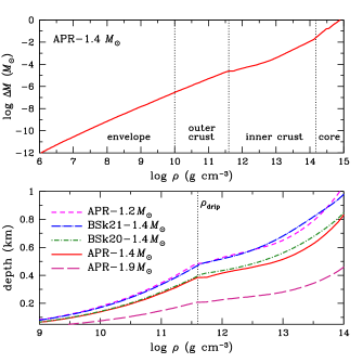
Figure 2: Accreted mass $\Delta M$ (top panel) and depth (bottom panel) as a function of density $\rho$. Vertical dotted lines indicate boundaries between envelope and crust (taken to be at $10^{10}\mbox{ g cm${}^{-3}$}$), outer and inner crust (at $\rho_{\rm drip}\approx 4\times 10^{11}\mbox{ g cm${}^{-3}$}$), and crust and core (at baryon density $n=0.09\mbox{ fm${}^{-3}$}$).

3 Fit to low braking index pulsars

The age of the three pulsars (PSR J0537$-$6910, B0833$-$45, and J1734$-$3333) with $n<1.5$ is in the range of $\approx 1$–16 kyr (see Table 1). Therefore, we seek a magnetic field growth timescale on this order. From eq. (2) and Fig. 2, we estimate that the magnetic field should be buried at a density $\sim 10^{11}\mbox{ g cm${}^{-3}$}$, which corresponds to an accreted mass $\Delta M\sim 10^{-5}M_{\odot}$.

Beginning with an initial condition which has the magnetic field $B_{0}$ buried at density $\rho_{\rm b}$, the induction equation [eq. (6)] is solved to obtain the radial profile of magnetic field as a function of time. Integrating eq. (1), we obtain the evolution of the spin period

$$P(t)=\left[P_{0}^{2}+\gamma\int_{t_{0}}^{t}B(R,t^{\prime})^{2}\,dt^{\prime}\right]^{1/2},$$ (7)

where $P_{0}$ is the initial pulsar spin period and $B(R,t)$ is the magnetic field at the NS surface at time $t$ and is given by our solution to the induction equation. From $P(t)$, we calculate its first and second time derivatives $\dot{P}(t)$ and $\ddot{P}(t)$, respectively, and corresponding braking index $n$ given by eq. (5). For each of the three pulsars, we vary the three initial conditions [$B_{0}$(G),$P_{0}$(s),$\log\rho_{\rm b}(\mbox{g cm${}^{-3}$})$] until the resulting $P$, $\dot{P}$, and $n$ match those of the pulsar at its current age. It is worth pointing out (see also Ho 2013b) that fitting to observables $P$ and $\dot{P}$ is equivalent to fitting to $\tau_{\rm c}$, $B$ as given by eq. (1), or spin-down luminosity since these are all formed from $P$ and $\dot{P}$ (see, e.g., Muslimov & Page 1996), while $n$ is an independent parameter since it includes $\ddot{P}$.

Figure 1 shows results for a set of initial conditions that fit each of the three pulsars: ($B_{0}$,$P_{0}$,$\log\rho_{\rm b}$) = ($3.4\times 10^{12}$,0.015,11.0) for J0537$-$6910, ($1.1\times 10^{13}$,0.066,11.5) for B0833$-$45, and ($1.3\times 10^{14}$,1.06,10.5) for J1734$-$3333. Each trajectory is labelled with the approximate age at which the calculated $P$, $\dot{P}$, and $n$ match their corresponding observed values. For J0537$-$6910, we obtain an age of 1.95 kyr, compared to its known age of $2_{-1}^{+3}\mbox{ kyr}$. Because of its young age, the current spin period $P=16\mbox{ ms}$ is not much different from the initial spin period $P_{0}=15\mbox{ ms}$. For B0833$-$45, we obtain an age of 10.2 kyr, compared to its known age of $11_{-5.6}^{+5}\mbox{ kyr}$. The spin period in this pulsar has increased significantly from 66 ms to the current 89 ms due to its much older age. For J1734$-$3333, we obtain an age of 2.07 kyr, compared to its minimum age of $>1.3\mbox{ kyr}$. Despite its similar age to J0537$-$6910, J1734$-$3333 underwent noticeable spin-down due to its much stronger magnetic field. Since $B\sim 10^{14}\mbox{ G}$ for J1734$-$3333, Hall effects and anisotropic conductivities may need to be taken into account, although these should not change our conclusions at a qualitative level. We also note the work of Gourgouliatos & Cumming (2015), who use numerical simulations to model Hall drift effects and obtain field growth with multipolar toroidal fields of the order of $10^{14}\mbox{ G}$ that can produce braking indices matching those observed.

Figure 3 shows relationships between the three initial conditions, $B_{0}$, $P_{0}$, and $\rho_{\rm b}$, as well as how initial values compare to present values. For a pulsar at a given age, the inferred density at which the magnetic field is initially buried depends on NS mass and nuclear EOS model, while $B_{0}$ and $P_{0}$ do not depend significantly on $M$ or EOS. The thicker the crust (see Fig. 2), the shallower the field needs to be buried to match current values of $P$, $\dot{P}$, and $n$. The shallower the field is buried, the closer the current magnetic field and spin period are to their initial values. Note that $B$ is evolving towards $B_{0}$, while $P$ is evolving away from $P_{0}$.

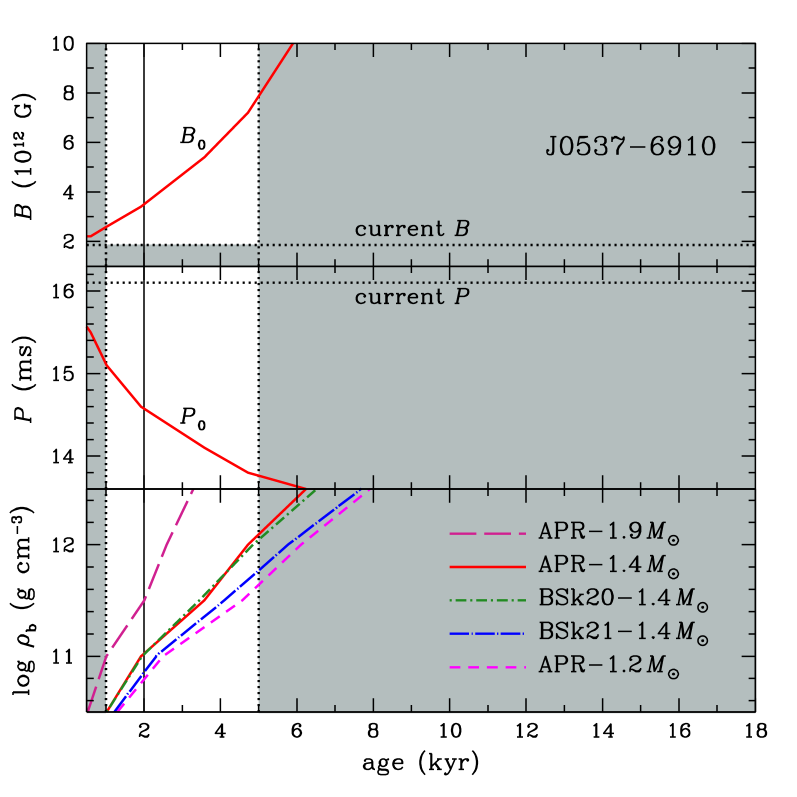
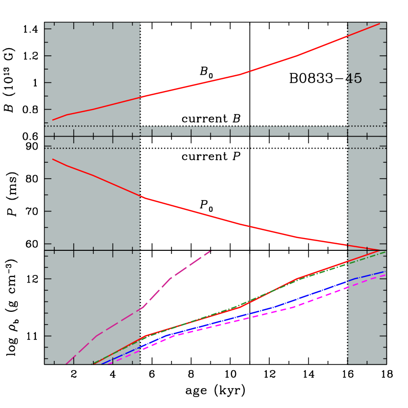
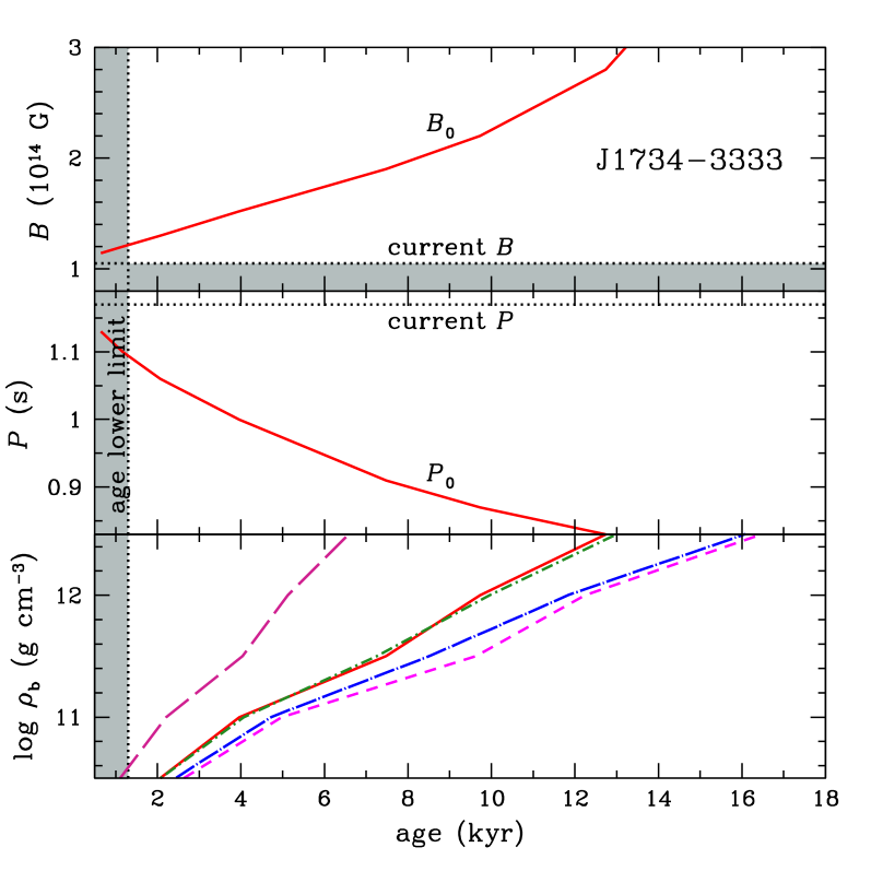
Figure 3: Initial magnetic field $B_{0}$ (top), initial spin period $P_{0}$ (centre), and burial density $\rho_{\rm b}$ (bottom) as a function of age for PSR J0537$-$6910 (left-hand panel), B0833$-$45 (centre panel), and J1734$-$3333 (right-hand panel). Horizontal dotted lines denote the current magnetic field $B$ and spin period $P$ of each pulsar, where the former is given by $B=6.4\times 10^{19}\mbox{ G }(P\dot{P})^{1/2}$. Vertical solid and dotted lines indicate the nominal age and age range, respectively, of each pulsar (see Table 1), except in the case of J1734$-$3333, the vertical dotted lines indicate the age lower limit.

More accurate age determinations would lead to tighter limits on the burial density (and hence mass accreted, via Fig. 2) and initial magnetic field and spin period. Current age estimates allow us to constrain the magnetic field strength at birth to within a factor of about three, i.e., $B_{0}\approx(3-7)\times 10^{12}\mbox{ G}$ for J0537$-$6910, $B_{0}\approx(0.9-1.3)\times 10^{13}\mbox{ G}$ for B0833$-$45, and $B_{0}\sim(1-3)\times 10^{14}\mbox{ G}$ for J1734$-$3333. These field strengths fall within the lognormal distributions determined from population synthesis studies, which find an average and width $\sigma$ of $\log B_{0}=12.95\pm 0.55$ in the case where there is no field decay (Faucher-Giguère & Kaspi, 2006; Guillón et al., 2014) and $\log B_{0}=13.25\pm 0.6$ in the case of where there is (model-dependent) field decay (Popov et al., 2010; Guillón et al., 2014). The initial spin periods are somewhat shorter for J0537$-$6910 and B0833$-$45 and much longer for J1734$-$3333 than the average found in these population synthesis studies, i.e., $P_{0}=0.30\pm 0.15\mbox{ s}$ (Faucher-Giguère & Kaspi, 2006) and $P_{0}=0.25\pm 0.1\mbox{ s}$ (Popov et al., 2010). However Guillón et al. (2014) find a much broader distribution, such that even $P_{0}\approx 1\mbox{ s}$ for J1734$-$3333 is within $2\sigma$ of the average value (see also Igoshev & Popov 2013).

4 Discussion

The standard theoretical scenario for spin evolution of isolated pulsars is one in which a pulsar loses its rotational energy via dipole radiation and slows down over time with a constant surface magnetic field, and this scenario works well to explain pulsars at an early age ($<10^{5}\mbox{ yr}$) and pulsars with braking index $n\approx 3$ (see Table 1). Here we study an alternative scenario, one in which the intrinsic magnetic field of a pulsar is buried by accretion soon after its birth in a supernova. Our scenario works alongside the standard scenario, by providing a natural explanation for pulsars with $n<3$. We fit observations of the three pulsars whose braking index $n<1.5$, i.e., PSR J0537$-$6910, B0833$-$45, and J1734$-$3333. We find that the mass required to bury the magnetic field is $\Delta M\sim 10^{-5}M_{\odot}$. Another requirement is that the timescale over which this mass is accreted must be shorter than the field diffusion timescale (Geppert et al., 1999), given approximately by eq. (2). Thus most newborn NSs probably fall within the standard scenario, with very little or no accretion. A relatively few, like the three examined here, quickly accreted enough mass to bury their magnetic field. Generally, the range of accreted mass could be quite large. Thus a third formation channel is one in which a large amount of matter is accreted. Such is possibly the case for the central compact objects (CCOs) studied in Ho (2011), where $\Delta M\gtrsim 10^{-4}M_{\odot}$. CCOs have age $<\mbox{ a few}\times 10^{4}\mbox{ yr}$, and their surface magnetic field is $\sim 10^{10}-10^{11}\mbox{ G}$ (Halpern & Gotthelf, 2010; Gotthelf et al., 2013a; Ho, 2013a).

Unification of different observational classes of NSs, such as magnetars, CCOs, and normal radio pulsars, via evolution of a NS from one class to another (Kaspi, 2010; Popov et al., 2010), would help alleviate the NS-supernova birthrate problem (Keane & Kramer, 2008). One pulsar studied here that is of particular interest in this regard is J1734$-$3333. Based on its current inferred magnetic field and braking index, this pulsar appears to be moving in Fig. 1 from the region populated by normal radio pulsars into that of magnetars (Espinoza et al., 2011b). We find that it has a magnetar-strength magnetic field at birth, i.e., $B_{0}\sim(1-3)\times 10^{14}\mbox{ G}$, with the exact value dependent on the age of the pulsar (see right-hand panel of Fig. 3). In the case of shallow field burial and no significant field decay during its life thus far, the magnetic field of J1734$-$3333 is nearly at its birth value and will reach it at an age $\approx 10^{4}\mbox{ yr}$. We point out that our projection of the trajectory of J1734$-$3333 is one that involves a braking index which changes over time (cf. Espinoza et al. 2011b). In particular, a detectable change from $n=0.9$ to $1$, based on the current uncertainty of 0.1, takes about 70 yr. J0537$-$6910 is perhaps a more promising target for observing a braking index change: a change from $n=-1.5$ to $-1.4$ takes about 20 yr. For completeness, the braking index change for Vela from $n=1.4$ to 1.5 takes about 400–500 yr. The difficulty lies with the much larger braking index uncertainty for these three (low braking index) pulsars compared to that of other pulsars (see Table 1). For example, evolution of braking index and third time derivative of spin period is observed for Crab (Lyne et al., 2015) and B1509$-$58 (Livingstone & Kaspi, 2011).

It is possibly noteworthy that two (J0537$-$6910 and Vela) of the three pulsars with $n<1.5$ undergo regular, large-amplitude glitches in their timing behaviour. The third (J1734$-$3333) recently had a large glitch, as reported in the Glitch Catalogue (Espinoza et al., 2011a). The other pulsars with $1.8<n<3$ either are not seen to glitch (B1509$-$58), have small amplitude glitches (e.g., Crab), or have glitches whose amplitude varies greatly (e.g., the magnetar J1846$-$0258) (see Table 1). The distinctiveness of J0537$-$6910 and Vela glitches is discussed by Espinoza et al. (2011a), who also show that glitch size has a bimodal distribution (see also Yu et al. 2013). The possible connection between low braking index and regular, large glitches in certain pulsars is noted by Espinoza (2013), who report another three pulsars (with $n=-1,2,$ and $2$) that could be in this group. These large amplitude spin-up glitches are of great interest since they may be revealing properties of the neutron superfluid in the NS (Baym et al., 1969; Anderson & Itoh, 1975; Alpar et al., 1984). The regularity of these similarly-sized glitches is thought to be the result of the pulsar tapping and exhausting the entire angular momentum reservoir of the superfluid in the NS inner crust (Link et al., 1999; Andersson et al., 2012; Chamel, 2013; Piekarewicz et al., 2014; Ho et al., 2015; Hooker et al., 2015; Steiner et al., 2015). Our simulations of magnetic field diffusion from the (inner and outer) crust to the surface suggest that perhaps this motion could be involved in triggering glitches of the type seen in low braking index pulsars.

If regular, large glitches are a symptom of a previously buried magnetic field, then glitch activity could be used as a criterion for searches for descendants of CCOs. Previous searches for CCOs and their descendants focus on the region in $P$–$\dot{P}$ phase space where known CCOs reside (see Fig. 1). These searches have thus far not found definitive candidates (Gotthelf et al., 2013b; Bogdanov et al., 2014; Luo et al., 2015). As we show here (see also Luo et al. 2015), pulsars with an emerging magnetic field move rapidly through this region of $P$–$\dot{P}$, and thus the likelihood of discovery here is low. This can also explain the relative paucity of pulsars here (Halpern & Gotthelf, 2010; Kaspi, 2010). Once their intrinsic fields reach the surface and these pulsars evolve to join the majority of the NS population, they might still be distinguished by their glitch activity. After all, glitch size and activity peak at age $\sim 10^{4}\mbox{ yr}$ (McKenna & Lyne, 1990; Espinoza et al., 2011a), and glitches only occur in pulsars with $\tau_{\rm c}\lesssim 10\mbox{ Myr}$ (Espinoza et al., 2011a).

Finally, it is well known that pulsar characteristic age $\tau_{\rm c}$ is often discrepant with true age, and thus the former can be an unreliable estimate of the latter (e.g., the case with CCOs). For seven of the nine braking index pulsars, the characteristic age is within a factor of about two of the true age (see Table 1), although some of the true age determinations are likely biased towards $\tau_{\rm c}$. Thus $\tau_{\rm c}$ is a relatively good age estimate for these types of sources and when these pulsars are near maximum $\dot{P}$ and post-maximum. Thus low $\tau_{\rm c}$ could be another possible criterion in searches for CCO descendants.

References

- Akmal et al. (1998) Akmal, A., Pandharipande, V.R., Ravenhall, D. G., 1998, Phys. Rev. C, 58, 1804
- Alpar et al. (1984) Alpar, M. A., Anderson, P. W., Pines, D., Shaham, J., 1984, ApJ, 276, 325
- Anderson & Itoh (1975) Anderson, P. W., Itoh, N., 1975, Nature, 256, 25
- Andersson et al. (2012) Andersson, N., Glampedakis, K., Ho, W. C. G., Espinoza, C. M., 2012, Phys. Rev. Lett., 109, 241103
- Antonopoulou et al. (2015) Antonopoulou, D., Weltevrede, P., Espinoza, C. M., Watts, A. L., Johnston, S., Shannon, R. M., Kerr, M., 2015, MNRAS, 447, 3924
- Baym et al. (1969) Baym, G., Pethick, C., Pines, D., Ruderman, M., 1969, Nature, 224, 872
- Bernal et al. (2010) Bernal, C. G., Lee, W. H., Page, D., 2010, Revista Mexicana de Astron. Astrof., 46, 301
- Bernal et al. (2013) Bernal, C. G., Page, D., Lee, W. H., 2013, ApJ, 770, 106
- Blanton & Helfand (1996) Blanton, E. L., Helfand, D. J., 1996, ApJ, 470, 961
- Bocchino et al. (2005) Bocchino, F., van der Swaluw, E., Chevalier, R., Bandiera, R. 2005, A&A, 442, 539
- Bogdanov et al. (2014) Bogdanov, S., Ng, C.-Y., Kaspi, V. M., 2014, ApJ, 792, L36
- Camilo et al. (2006) Camilo, F., Ransom, S. M., Gaensler, B. M., Slane, P. O., Lorimer, D. R., Reynolds, J., Manchester, R. N., Murray, S. S., 2006, ApJ, 637, 456
- Chamel (2013) Chamel, N., 2013, Phys. Rev. Lett., 110, 011101
- Chen et al. (2006) Chen, Y., Wang, Q. D., Gotthelf, E. V., Jiang, B., Chu, Y.-H., Gruendl, R., 2006, ApJ, 651, 237
- Chevalier (1989) Chevalier, R. A., 1989, ApJ, 346, 847
- Colpi et al. (2000) Colpi, M., Geppert, U., Page, D., 2000, ApJ, 529, L29
- Contopoulos et al. (2014) Contopoulos, I., Kalapotharakos, C., Kazanas, D., 2014, ApJ, 781, 46
- Espinoza (2013) Espinoza, C. M., 2013, in van Leeuwen, J., ed, Proc. IAU Symp. 291, Neutron Stars and Pulsars: Challenges and Opportunities After 80 Years. Cambridge University Press, Cambridge, p. 195
- Espinoza et al. (2011a) Espinoza, C. M., Lyne, A. G., Stappers, B. W., Kramer, M., 2011a, MNRAS, 414, 1679
- Espinoza et al. (2011b) Espinoza, C. M., Lyne, A. G., Kramer, M., Manchester, R. N., Kaspi, V. M. 2011b, ApJ, 741, L13
- Faucher-Giguère & Kaspi (2006) Faucher-Giguère, C.-A., Kaspi, V. M. 2006, ApJ, 643, 332
- Gaensler et al. (1999) Gaensler, B. M., Brazier, K. T. S., Manchester, R. N., Johnston, S., Green, A. J., 1999, MNRAS, 305, 724
- Geppert et al. (1999) Geppert, U., Page, D., Zannias, T., 1999, A&A, 345, 847
- Glampedakis et al. (2011) Glampedakis, K., Jones, D. I., Samuelsson, L., 2011, MNRAS, 413, 2021
- Goldreich & Reisenegger (1992) Goldreich, P. Reisenegger, A., 1992, ApJ, 395, 250
- Gotthelf et al. (2013a) Gotthelf, E. V., Halpern, J. P., Alford, J., 2013a, ApJ, 765, 58
- Gotthelf et al. (2013b) Gotthelf, E. V., Halpern, J. P., Allen, B., Knispel, B., 2013b, ApJ, 773, 141
- Gourgouliatos & Cumming (2015) Gourgouliatos, K. N., Cumming, A., 2015, MNRAS, 446, 1121
- Gradari et al. (2011) Gradari, S., et al., 2011, MNRAS, 412, 2689
- Guillón et al. (2014) Guillón, M., Miralles, J. A., Viganò, D., Pons, J. A., 2014, MNRAS, 443, 1891
- Güneydaş & Ekşi (2013) Güneydaş, A., Ekşi, K. Y. 2013, MNRAS, 430, L59
- Gunn & Ostriker (1969) Gunn, J. E., Ostriker, J. P. 1969, Nature, 221, 454
- Halpern & Gotthelf (2010) Halpern, J. P., Gotthelf, E. V., 2010, ApJ, 709, 436
- Hamil et al. (2015) Hamil, O., Stone, J. R., Urbanec, M., Urbancová, G., 2015, Phys. Rev. D, 91, 063007
- Ho (2011) Ho, W. C. G., 2011, MNRAS, 414, 2567
- Ho (2013a) Ho, W. C. G., 2013a, in van Leeuwen, J., ed, Proc. IAU Symp. 291, Neutron Stars and Pulsars: Challenges and Opportunities After 80 Years. Cambridge University Press, Cambridge, p. 101
- Ho (2013b) Ho, W. C. G., 2013b, MNRAS, 429, 113
- Ho & Andersson (2012) Ho, W. C. G., Andersson, N., 2012, Nature Phys., 8, 787
- Ho et al. (2015) Ho, W. C. G., Espinoza, C. M., Antonopoulou, D., Andersson, N., 2015, Science Adv., submitted
- Hooker et al. (2015) Hooker, J., Newton, W. G., Li, B.-A., 2015, MNRAS, 449, 3559
- Horowitz et al. (2015) Horowitz, C. J., Berry, D. K., Briggs, C. M., Caplan, M. E., Cumming, A., Schneider, A. S., 2015, Phys. Rev. Lett., 114, 031102
- Igoshev & Popov (2013) Igoshev, A. P., Popov, S. B., 2013, MNRAS, 432, 967
- Igoshev & Popov (2014) Igoshev, A. P., Popov, S. B., 2014, MNRAS, 444, 1066
- Kaspi (2010) Kaspi, V. M., 2010, Publ. Natl. Acad. Sci., 107, 7147
- Keane & Kramer (2008) Keane, E. F., Kramer, M., 2008, MNRAS, 391, 2009
- Kumar et al. (2012) Kumar, H. S., Safi-Harb, S., Gonzalez, M. E., 2012, ApJ, 754, 96
- Link et al. (1999) Link, B., Epstein, R. I., Lattimer, J. M., 1999, Phys. Rev. Lett., 83, 3362
- Livingstone & Kaspi (2011) Livingstone, M. A., Kaspi, V. M., 2011, ApJ, 742, 31
- Livingstone et al. (2007) Livingstone, M. A., Kaspi, V. M., Gavriil, F. P., Manchester, R. N., Gotthelf, E. V. G., Kuiper, L., 2007, Ap&SS, 308, 317
- Livingstone et al. (2011) Livingstone, M. A., Ng, C.-Y., Kaspi, V. M., Gavriil, F. P., Gotthelf, E. V., 2011, ApJ, 730, 66
- Luo et al. (2015) Luo, J., Ng, C.-Y., Ho, W. C. G., Bogdanov, S., Kaspi, V. M., He, C., 2015, ApJ, in press
- Lyne et al. (1993) Lyne, A. G., Pritchard, R. S., & Graham-Smith, F. 1993, MNRAS, 265, 1003
- Lyne et al. (2013) Lyne, A., Graham-Smith, F., Weltevrede, P., Jordan, C., Stappers, B., Bassa, C., Kramer, M., 2013, Science, 342, 598
- Lyne et al. (2015) Lyne, A. G., Jordan, C. A., Graham-Smith, F., Espinoza, C. M., Stappers, B. W., Weltevrede, P., 2015, MNRAS, 446, 857
- Lyne et al. (1996) Lyne, A. G., Pritchard, R. S., Graham-Smith, F., Camilo, F., 1996, Nature, 381, 497
- McKenna & Lyne (1990) McKenna, J., Lyne, A. G., 1990, Nature, 343, 349
- Manchester et al. (2005) Manchester, R. N., Hobbs, G. B., Teoh, A., Hobbs, M., 2005, AJ, 129, 1993
- Middleditch et al. (2006) Middleditch, J., Marshall, F. E., Wang, Q. D., Gotthelf, E. V., Zhang, W., 2006, ApJ, 652, 1531
- Muslimov & Page (1996) Muslimov, A., Page, D., 1996, ApJ, 458, 347
- Page et al. (2009) Page, D., Lattimer, J. M., Prakash, M., Steiner, A. W., 2009, ApJ, 707, 1131
- Park et al. (2010) Park, S., Hughes, J. P., Slane, P. O., Mori, K., Burrows, D. N., 2010, ApJ, 710, 948
- Piekarewicz et al. (2014) Piekarewicz, J., Fattoyev, F.J., Horowitz, C. J., 2014, Phys. Rev. C, 90, 015803
- Pons et al. (2013) Pons, J. A., Viganò, D., Rea, N., 2013, Nature Phys., 9, 431
- Popov et al. (2010) Popov, S. B., Pons, J. A., Miralles, J. A., Boldin, P. A., Posselt, B., 2010, MNRAS, 401, 2675
- Potekhin et al. (2013) Potekhin, A. Y., Fantina, A. F., Chamel, N., Pearson, J. M., Goriely, S., 2013, A&A, 560, A48
- Potekhin et al. (2015) Potekhin, A. Y., Pons, J. A., Page, D., 2015, Space Sci. Rev., submitted
- Roy et al. (2012) Roy, J., Gupta, Y., Lewandowski, W., 2012, MNRAS, 424, 2213
- Spitkovsky (2006) Spitkovsky, A., 2006, ApJ, 648, L51
- Steiner et al. (2015) Steiner, A. W., Gandolfi, S., Fattoyev, F. J., Newton, W. G., 2015, Phys. Rev. C, 91, 015804
- Tsuruta et al. (2009) Tsuruta, S., Sadino, J., Kobelski, A., Teter, M. A., Liebmann, A. C., Takatsuka, T., Nomoto, K., Umeda, H., 2009, ApJ, 691, 621
- Urpin & Muslimov (1992) Urpin, V., Muslimov, A. G., 1992, MNRAS, 256, 261
- Viganò & Pons (2012) Viganò, D., Pons, J. A., 2012, MNRAS, 425, 2487
- Viganò et al. (2013) Viganò, D., Rea, N., Pons, J. A., Perna, R., Aguilera, D. N., Miralles, J. A., 2013, MNRAS, 434, 123
- Wang & Gotthelf (1998) Wang, Q. D., Gotthelf, E. V., 1998, ApJ, 494, 623
- Weltevrede et al. (2011) Weltevrede, P., Johnston, S., Espinoza, C. M., 2011, MNRAS, 411, 1917
- Yu et al. (2013) Yu, M., et al., 2013, MNRAS, 429, 688