The dynamical impact of a shortcut in unidirectionally coupled rings of oscillators

Abstract

We study the destabilization mechanism in a unidirectional ring of identical oscillators, perturbed by the introduction of a long-range connection. It is known that for a homogeneous, unidirectional ring of identical Stuart-Landau oscillators the trivial equilibrium undergoes a sequence of Hopf bifurcations eventually leading to the coexistence of multiple stable periodic states resembling the Eckhaus scenario. We show that this destabilization scenario persists under small non-local perturbations. In this case, the Eckhaus line is modulated according to certain resonance conditions. In the case when the shortcut is strong, we show that the coexisting periodic solutions split up into two groups. The first group consists of orbits which are unstable for all parameter values, while the other one shows the classical Eckhaus behavior.

¹Humboldt-University of Berlin, Institute of Mathematics, Unter den Linden 6, 10099 Berlin, Germany

1 Introduction

The theory of dynamics on networks is a rapidly growing field of research. Motivated by applications from neuroscience, biological systems, and social networks, scientists from various areas have investigated the connection between network structure and dynamics in the last few decades. Since then, the importance of special topologies like scale-free or small world networks was discovered and dynamics on these structures were studied extensively [1].

In this article, we study a special class of network topologies, namely unidirectional rings which are perturbed by the insertion of a single additional non-local link [Fig. 1]. One reason for the interest in ring structures is that they emerge in many natural systems [2, 3, 4]. Also, rings can be seen as motifs of larger and more complex networks [5]. A lot of research has been done for bidirectional rings in the last few years [6, 7, 8, 9, 10]. In contrary, less is known about dynamics in unidirectional rings [11, 12, 13, 14, 15, 16], although these structures play an important role in various applications [17, 18, 19, 4, 20, 21]. As a simple, paradigmatic model, we consider unidirectional rings of $N$ identical Stuart-Landau oscillators with an additional shortcut from node $\ell$ to node $N$, to which we refer as a perturbation of the homogeneous system. The dynamics on the perturbed ring are described by the following equations:

$$\dot{z}_{j}\left(t\right) = \left(\mu-\left|z_{j}\left(t\right)\right|^{2}\right)z_{j}+z_{j+1}\left(t\right),\quad j=1,...,N-1,$$

$$\dot{z}_{N}\left(t\right) = \left(\mu-\left|z_{N}\left(t\right)\right|^{2}\right)z_{N}+z_{1}\left(t\right)+sz_{\ell}\left(t\right),$$ (1)

where $\mu=\alpha+i\beta$, $\beta>0$, $s>0$ is the shortcut strength, and $z_{j}\left(t\right)\in\mathbb{C}$. For an unperturbed ring ($s=0$), the destabilization mechanism is described in [14]. In particular, when the parameter $\alpha=\Re\left(\mu\right)$ in (1) is increased, the zero equilibrium

$$z_{1}=...=z_{N}=0$$ (2)

loses stability and undergoes a sequence of Hopf bifurcations. The first half of the emerging branches of periodic solutions stabilizes at appropriate values of $\alpha$ (see chapter 2.2). Remarkably, this phenomenon resembles the Eckhaus scenario in spatially extended diffusive systems [22, 23]. The aim of this article is to investigate the transformation of this scenario under non-local perturbations which destroy the rotational symmetry of the system. We investigate two different asymptotic cases of small and large perturbation size $s$. For small $s$, the Eckhaus scenario persists qualitatively with a modulated Eckhaus line, while for large $s$, there is a qualitative difference to the unperturbed case that reflects the new network topology, i.e. the existence of a new loop.

The article is structured as follows. In section 2 we discuss the stability of the zero solution (2), its spectrum and its bifurcations. In section 3 we find asymptotic expressions for the emerging periodic solutions in the case of small perturbation size $s$. We also reduce the case of asymptotically large $s$ to the analysis of an inhomogeneous ring. Section 4 deals with the stability analysis of the periodic solutions and the results are compared to numerical simulations. Finally, we discuss our findings and give an outlook on possible extensions and applications of the results in section 5.

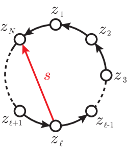
Figure 1: Coupling scheme of a unidirectional ring with a shortcut.

2 Stability of the zero solution

To study the stability of system (1) it is convenient to identify each variable $z_{j}\left(t\right)\in\mathbb{C}$ with a two-dimensional real variable $\boldsymbol{z}_{j}\left(t\right)=\left(z_{j,1}\left(t\right),z_{j,2}\left(t\right)\right)^{\top}=\left(\Re\left(z_{j}\left(t\right)\right),\Im\left(z_{j}\left(t\right)\right)\right)^{\top}\in\mathbb{R}^{2}$. Then, system (1) is equivalent to the real system

$$\dot{\boldsymbol{z}}_{j}\left(t\right) = \left(M_{\mu}-\left(z_{j,1}^{2}+z_{j,2}^{2}\right)\right)\boldsymbol{z}_{j}+\boldsymbol{z}_{j+1},$$

$$\dot{\boldsymbol{z}}_{N}\left(t\right) = \left(M_{\mu}-\left(z_{N,1}^{2}+z_{N,2}^{2}\right)\right)\boldsymbol{z}_{N}+\boldsymbol{z}_{1}+s\boldsymbol{z}_{\ell},$$ (3)

where $M_{\mu}=\left[\begin{matrix}\alpha&-\beta\\ \beta&\alpha\end{matrix}\right]$ is the representation of the multiplication with $\mu$ in $\mathbb{R}^{2\times 2}$.

2.1 Spectrum of the equilibrium

We linearize system (3) in $\boldsymbol{z}_{1}=..=\boldsymbol{z}_{N}\equiv 0$ and obtain the variational equation

$$\frac{d}{dt}\delta\boldsymbol{z}_{j}\left(t\right) =M_{\mu}\delta\boldsymbol{z}_{j}+\delta\boldsymbol{z}_{j+1}\left(t\right),\ j=1,...,N-1,$$

$$\frac{d}{dt}\delta\boldsymbol{z}_{N}\left(t\right) =M_{\mu}\delta\boldsymbol{z}_{N}+\delta\boldsymbol{z}_{1}\left(t\right)+s\delta\boldsymbol{z}_{\ell}\left(t\right),$$

which can be written as

$$\frac{d}{dt}\delta Z\left(t\right)=\left[\mathrm{Id}_{N}\otimes M_{\mu}+G_{s}\otimes\mathrm{Id}_{2}\right]\delta Z\left(t\right),$$ (4)

where $\delta Z=\left(\delta\boldsymbol{z}_{1},...,\delta\boldsymbol{z}_{N}\right)^{\top}$, $\mathrm{Id}_{N}\in\mathbb{R}^{N\times N}$ is the $N$-dimensional identity matrix,

$$G_{s}=\left[\begin{array}[]{cccc}0&1&&0\\ \vdots&\ddots&\ddots\\ 0&&\ddots&1\\ 1&0&s&0\end{array}\right]$$ (5)

is the coupling matrix of the perturbed ring, $A\otimes B$ denotes the tensor product of the two matrices $A$ and $B$. Equation (4) is a simple example of a system, which is treatable by a master stability function (MSF) approach [24]. In our case the MSF $M:\mathbb{C}\longrightarrow\mathbb{R}$ simply reads $M\left(\lambda\right)=\alpha+\Re\left(\lambda\right)$, where $\lambda$ is an eigenvalue of the coupling matrix $G_{s}$. Indeed, the spectrum of (4) is

$$\sigma\left(\mathrm{Id}_{N}\otimes M_{\mu}+G_{s}\otimes\mathrm{Id}_{2}\right)=\sigma\left(M_{\mu}\right)+\sigma\left(G_{s}\right)=\left\{\mu,\bar{\mu}\right\}+\sigma\left(G_{s}\right).$$ (6)

Taking the real part, we obtain $M\left(\lambda\right)=\alpha+\Re\left(\lambda\right)$. The spectrum of the coupling matrix $G_{s}$ equals the set of solutions of the characteristic equation

$$\chi_{G_{s}}\left(\lambda\right)=\lambda^{N}-s\lambda^{\ell-1}-1=0.$$ (7)

For $s=0$, $\sigma\left(G_{0}\right)$ consists of the $N$ roots of unity

$$\gamma_{N,k}=e^{i\frac{2\pi k}{N}},\ k=0,...,N-1.$$

For small $s\neq 0$, the roots $\lambda_{k}$, $k=1,...,N$, of eq. (7) are given (asymptotically) as

$$\lambda_{k}\left(s\right)=\gamma_{N,k}+\frac{s}{N}\gamma_{N,k}^{\ell}+{\cal O}\left(s^{2}\right),$$ (8)

as one can readily compute by applying the implicit function theorem to (7) with base points $(s_{0},\lambda_{0})=(0,\gamma_{N,k})$. Hence, the spectrum of $G_{s}$ is a weak modulation of the spectrum of the circulant matrix $G_{0}$ [see Fig. 2(a), (b)]. For large $s$, $\sigma\left(G_{s}\right)$ can be computed in a similar manner. In Appendix A we show that in this case the spectrum of $G_{s}$ splits into two parts: there are $\ell-1$ roots

$$\lambda_{1,k}\left(s\right)\approx s^{-\nicefrac{{1}}{{\ell-1}}}\gamma_{\ell-1,k},\ k=0,...,\ell-2,$$ (9)

located close to an inner circle of amplitude $\sim s^{-\nicefrac{{1}}{{\ell-1}}}$ and $N-\ell+1$ roots

$$\lambda_{2,k}\left(s\right)\approx s^{\nicefrac{{1}}{{N-\ell+1}}}\gamma_{N-\ell+1,k},\ k=0,...,N-\ell,$$ (10)

which are close to an outer circle of amplitude $\sim s^{\nicefrac{{1}}{{N-\ell+1}}}$ [see Fig. 2].

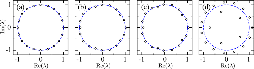
Figure 2: Spectra of the coupling matrix $G_{s}$ (5) for $N=20$ oscillators, a shortcut at node $\ell=6$ and for different coupling strengths $s$: a) $s=0.1$, b) $s=0.6$, c) $s=1$, d) $s=5$.

2.2 Bifurcations of the equilibrium

From the formula (6) for the spectrum of the equilibrium $\boldsymbol{z}_{1}=..=\boldsymbol{z}_{N}\equiv 0$, it follows that it is asymptotically stable iff

$$\Re\left(\lambda\right)<-\alpha,\ \text{for all }\lambda\in\sigma\left(G_{s}\right).$$ (11)

When the parameter $\alpha$ is increased starting from a value which satisfies (11), a bifurcation takes place whenever for some $\lambda\in\sigma\left(G_{s}\right)$:

$$\alpha=-\Re\left(\lambda\right).$$ (12)

Note that there is always one purely real eigenvalue $\lambda_{1}\left(s\right)=1+\frac{s}{N}+{\cal O}\left(s^{2}\right)$ of $G_{s}$ which has maximal real part among all eigenvalues of $G_{s}$. Indeed, for any solution $\lambda=\varrho e^{i\varphi}$, $\varrho\geq 0$, of (7), we have

$$1=\left|\varrho^{N}e^{iN\varphi}-s\varrho^{\ell-1}e^{i\left(\ell-1\right)\varphi}\right|\geq\varrho^{N}-s\varrho^{\ell-1}=\chi_{G_{s}}\left(\varrho\right)+1.$$

Hence, $\chi_{G_{s}}\left(\varrho\right)\leq 0$, and $\lim_{x\to\infty}\chi_{G_{s}}\left(x\right)=+\infty$ implies that there exists a real solution $\varrho_{0}\geq\varrho$ such that $\chi_{G_{s}}\left(\varrho_{0}\right)=0$. Therefore, for small $s\geq 0$ the equilibrium switches stability at

$$\alpha_{1}\left(s\right)\approx-\left(1+\frac{s}{N}\right).$$

Since we assume $\beta\neq 0$, this bifurcation is a Hopf bifurcation and the emerging periodic orbit has frequency $\beta$ at onset. As for $s=0$, the bifurcation is supercritical for small $s>0$, because the cubic term of the corresponding normal form depends continuously on $s$. Therefore, a branch of stable periodic solutions emerges and exists for $\alpha>\alpha_{1}\left(s\right)$. A further increase of $\alpha$ leads to a sequence of Hopf bifurcations which give rise to $N-1$ branches of periodic solutions. As in the case $s=0$, all bifurcations are supercritical if $s>0$ is small (by continuity). The same is true if $s>0$ is large, as we show in Appendix B. The latter $N-1$ periodic solutions are initially unstable, inheriting instability from the steady state. The initial frequency $\omega$ of the emerging periodic solution equals the imaginary part of the crossing eigenvalue, that is $\omega=\beta+\Im\left(\lambda\right)$ for the corresponding $\lambda\in G_{s}$. For the unperturbed ring ($s=0$) the first $\left\lfloor(N-1)/2\right\rfloor$ ($\left\lfloor x\right\rfloor:=\max\left\{n\in\mathbb{N}:\,n\leq x\right\}$) branches stabilize when they cross the Eckhaus stabilization line [14]

$$\frac{1}{N}|Z|^{2}=\frac{3\alpha}{4}+\sqrt{\left(\frac{\alpha}{4}\right)^{2}+\frac{1}{2}},$$ (13)

where $\left|Z\right|^{2}$ is the (constant) amplitude of a periodic solution $Z\left(t\right)=(z_{1}\left(t\right),...,z_{N}\left(t\right))^{T}$. This observation is in striking analogy with the well known Eckhaus destabilization in diffusive systems [22, 23]. Remarkably, it is also found in this unidirectional system which does not extend to a spatially extended system in a natural manner. In section 4 we investigate how the added shortcut changes this scenario.

3 Emergent periodic orbits

Let $Z\left(t\right)$ be a periodic solution of (1), which emerges from a Hopf bifurcation at

$$\alpha\left(s\right)=-\Re\left(\lambda\left(s\right)\right),$$ (14)

and which is associated to the eigenvalue $\lambda\left(s\right)$ of the coupling matrix $G_{s}$, see (8)–(10). Because of the $S^{1}$-symmetry of the system, we employ the ansatz

$$Z\left(t\right)=\sqrt{\varepsilon}e^{i\omega\left(\varepsilon,s\right)t}V\left(\varepsilon,s\right),$$ (15)

where

$$\varepsilon:=\alpha-\alpha\left(s\right)\geq 0$$ (16)

is the parameter distance from the bifurcation point,

$$V\left(\varepsilon,s\right)=\left(v_{1}\left(\varepsilon,s\right),...,v_{N}\left(\varepsilon,s\right)\right)^{T}\in\mathbb{C}^{N},$$ (17)

is the profile vector and the frequency $\omega\left(\varepsilon,s\right)$ of $Z\left(t\right)$ is

$$\omega\left(\varepsilon,s\right)=\beta+\Im\left(\lambda\left(s\right)\right)+{\cal O}\left(\varepsilon\right).$$ (18)

The emerging periodic orbit is $\varepsilon$-close to the complex plane spanned by the eigenvector $b\left(s\right)$ of $G_{s}$ corresponding to $\lambda\left(s\right)$ and tangential at the bifurcation point itself [25]. This means, $V\left(0,s\right)=b\left(s\right)$ with

$$b\left(s\right)=a\left(s\right)\cdot\left(1,\lambda\left(s\right),\lambda^{2}\left(s\right),...,\lambda^{N-1}\left(s\right)\right)^{T},$$ (19)

where one may assume $a\left(s\right)\in\mathbb{R}$ due to the $S^{1}$-symmetry of the system. Figure 3 shows several examples of the profile shapes for different $s$ and $\lambda$. For $\left|\lambda\right|>1$ the emerging solutions become stronger localized at the $N$-th node $z_{N}$ with increasing $s$ since it scales as $z_{N}\sim\lambda^{N-1}$. For $\left|\lambda\right|<1$, the localization takes place at $z_{1}\left(t\right)$ for the same reason.

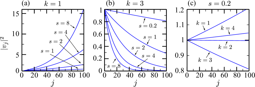
Figure 3: Moduli of the components of the initial profiles $V\left(0,s\right)=b\left(s\right)$ of emerging periodic solutions [see (17) and (19)] for different wave numbers $k$ (i.e., different eigenvalues $\lambda_{k}\left(s\right)$ of $G_{s}$) and coupling strengths $s$ as indicated in the figure. For all panels: $N=100$ and $\ell=26$.

3.1 Case I: small perturbation

In this section we consider $s$ to be small. Our aim is to determine a formal asymptotic expansion for the frequencies (18) and the profiles (17) of the periodic solutions and to derive evaluable approximate conditions for their stability. In particular, we are interested in the deformation of the Eckhaus stabilization line (13). In order to obtain asymptotic expressions for the profiles in case that $s,\varepsilon>0$, we linearize the vector field in $\varepsilon=s=0$. For a periodic solution (15), we introduce rescaled, rotating coordinates $u_{j}\left(t\right)\in\mathbb{C}$, $j=1,...,N$ according to

$$z_{j}=\sqrt{\varepsilon}e^{i\omega t}v_{j}u_{j},$$ (20)

with $\omega=\omega\left(\varepsilon,s\right)$ and $v_{j}=v_{j}\left(\varepsilon,s\right)$. Then (1) becomes

$$\dot{u}_{j} =\left(\alpha+i\left(\beta-\omega\right)-\varepsilon\left|v_{j}u_{j}\right|^{2}\right)u_{j}+\frac{v_{j+1}}{v_{j}}u_{j+1},$$ (21)

$$\dot{u}_{N} =\left(\alpha+i\left(\beta-\omega\right)-\varepsilon\left|v_{N}u_{N}\right|^{2}\right)u_{N}+\frac{v_{1}}{v_{N}}u_{1}+s\frac{v_{\ell}}{v_{N}}u_{\ell},$$ (22)

In rotating coordinates, the equilibrium solution

$$u_{j}\equiv 1,\ j=1,...,N,$$ (23)

corresponds to the periodic solution (15) of (1) and the stability of (15) and (23) is the same. In Appendix D we show that for each eigenvalue $\lambda_{k}\left(s\right)=\gamma_{N,k}+\frac{s}{N}\gamma_{N,k}^{\ell}+{\cal O}\left(s^{2}\right)$ of $G_{s}$, the corresponding branch of periodic solutions has frequencies

$$\omega_{k}\left(\varepsilon,s\right)=\beta+\Im\left(\gamma_{N,k}\right)+\frac{s}{N}\Im\left(\gamma_{N,k}^{\ell}\right)+{\cal O}\left(\left(\left|\varepsilon\right|+\left|s\right|\right)^{2}\right),$$ (24)

and profiles

$$v_{j}\left(\varepsilon,s\right)=\gamma_{N,k}^{j-1}\left(1+s\frac{j-1}{N}\gamma_{N,k}^{\ell-1}\right)+{\cal O}\left(\left(\left|\varepsilon\right|+\left|s\right|\right)^{2}\right).$$ (25)

3.2 Case II: large perturbation

In this section we consider $s$ to be large. To treat (1) as a weakly perturbed system we perform a change of variables

$$y_{j}\left(t\right)=\varsigma^{j}z_{j}\left(\varsigma^{2N}t\right),$$ (26)

with a small parameter $\varsigma=s^{-\nicefrac{{1}}{{N-\ell+1}}}$, which is the inverse radius of the outer spectral circle of eigenvalues (10). This transformation normalizes the emerging profiles (19) corresponding to the eigenvalues (10). The transformed variables (26) satisfy

$$\dot{y}_{j}\left(t\right) = \left(\varsigma^{2N}\mu-\varsigma^{2\left(N-j\right)}\left|y_{j}\left(t\right)\right|^{2}\right)y_{j}\left(t\right)+\varsigma^{2N-1}y_{j}\left(t\right),\ j=1,...,N-1,$$

$$\dot{y}_{N}\left(t\right) = \left(\varsigma^{2N}\mu-\left|y_{N}\left(t\right)\right|^{2}\right)y_{N}\left(t\right)+\varsigma^{3N-1}y_{1}+\varsigma^{2N-1}y_{\ell}\left(t\right).$$ (27)

Since $\varsigma^{3N-1}y_{1}=\varsigma^{N}\left(\varsigma^{2N-1}y_{1}\right)$ and $\varsigma^{N}$ is small, we consider system (27) as a small perturbation of

$$\dot{y}_{j}\left(t\right) = \left(\varsigma^{2N}\mu-\varsigma^{2\left(N-j\right)}\left|y_{j}\left(t\right)\right|^{2}\right)y_{j}\left(t\right)+\varsigma^{2N-1}y_{j}\left(t\right),\ j=1,...,N-1,$$

$$\dot{y}_{N}\left(t\right) = \left(\varsigma^{2N}\mu-\left|y_{N}\left(t\right)\right|^{2}\right)y_{N}\left(t\right)+\varsigma^{2N-1}y_{\ell}\left(t\right).$$ (28)

Although we cannot show that results for the persistence of hyperbolic invariant manifolds [26] apply and assure that (28) possesses the same hyperbolic invariant manifolds as does (27), the truncated system (28) is a natural approximation to (27). Note that in (28) the components $y_{1},\,...,\,y_{\ell-1}$ do not couple back to the rest of the system since the weak link from $y_{1}$ to $y_{N}$ was taken out. Therefore, the dynamics of the subsystem $y_{\ell},\,...,\,y_{N}$ is independent and, apart from the zero solution, acts as a periodic force on the attached subsystem $y_{1},\,...,\,y_{\ell-1}$. In original variables (28) reads

$$\dot{z}_{j}\left(t\right) = \left(\mu-\left|z_{j}\left(t\right)\right|^{2}\right)z_{j}+z_{j+1}\left(t\right),\ j=1,...,N-1,$$

$$\dot{z}_{N}\left(t\right) = \left(\mu-\left|z_{N}\left(t\right)\right|^{2}\right)z_{N}+sz_{\ell}\left(t\right).$$ (29)

The linearization of (29) at the zero solution has eigenvalues

$$\mu+\nu,\ \,\text{and}\,\ \bar{\mu}+\nu$$

where $\nu$ is a root of the characteristic equation

$$\left(\nu^{N-\ell+1}-s\right)\nu^{\ell-1}=0$$

of the reduced coupling matrix $H_{s}$, which is obtained by erasing the link from $z_{1}$ to $z_{N}$ from $G_{s}$. It has eigenvalues

$$\nu=0\ \,\text{and}\ \,\nu=s^{\nicefrac{{1}}{{N-\ell+1}}}\gamma_{N-\ell+1,k},\ k=1,...,N-\ell+1.$$ (30)

Periodic orbits which correspond to the algebraically $\left(\ell-1\right)$-fold eigenvalue $\nu=0$ are localized on the nodes $z_{1},\,...,\,z_{\ell-1}$.

4 Stability of the periodic orbits

4.1 Case I: small perturbation

The variational equation for system (21)–(22) at the stationary solution (23) is

$$\dot{u}_{j} = \left(\alpha+\varepsilon+i\left(\beta-\omega\right)-2\varepsilon\left|v_{j}\right|^{2}\right)u_{j}+\frac{v_{j+1}}{v_{j}}u_{j+1},$$

$$\dot{u}_{N} = \left(\alpha+\varepsilon+i\left(\beta-\omega\right)-2\varepsilon\left|v_{N}\right|^{2}\right)u_{N}+\frac{v_{1}}{v_{N}}u_{1}+s\frac{v_{\ell}}{v_{N}}u_{\ell}.$$

We transform the system into $\mathbb{R}^{2N}$ ($\boldsymbol{x}_{j}=(\Re(u_{j}),\Im(u_{j}))^{T}$) and insert the expansions (24) and (25) to obtain

$$\dot{\boldsymbol{x}}_{j} = -\left[M_{\tilde{\lambda}}+2\varepsilon\boldsymbol{\delta}_{11}\right]\boldsymbol{x}_{j}+M_{\tilde{\lambda}}\boldsymbol{x}_{j+1}+{\cal O}\left(\left(\left|\varepsilon\right|+\left|s\right|\right)^{2}\right)$$

$$\dot{\boldsymbol{x}}_{N} = -\left[M_{\tilde{\lambda}}+2\varepsilon\boldsymbol{\delta}_{11}\right]\dot{\boldsymbol{x}}_{N}+M_{\tilde{\lambda}}\dot{\boldsymbol{x}}_{1}+sM_{\lambda_{0}^{\ell}}\left[\dot{\boldsymbol{x}}_{\ell}-\dot{\boldsymbol{x}}_{1}\right]+{\cal O}\left(\left(\left|\varepsilon\right|+\left|s\right|\right)^{2}\right)$$ (31)

with $\lambda_{0}=\gamma_{N,k}$, $\tilde{\lambda}\left(s\right)=\lambda_{0}+\frac{s}{N}\lambda_{0}^{\ell}$, the matrix representation $M:\mathbb{C}\to\mathbb{R}^{2\times 2}$ [as in (3)] and $\boldsymbol{\delta}_{mn}=\left(\delta_{jm}\delta_{kn}\right)_{j,k}$ is the matrix which has the entry $1$ at position $\left(j,k\right)$ and zeros everywhere else. We drop the higher order terms in (31) and write the system in the form

$$\dot{\boldsymbol{X}}=A\left(\varepsilon,s\right)\boldsymbol{X}=\left[-\mathrm{Id}_{N}\otimes\left(M_{\tilde{\lambda}}+2\varepsilon\boldsymbol{\delta}_{11}\right)+G_{0}\otimes M_{\tilde{\lambda}}+\left(\boldsymbol{\delta}_{N1}-\boldsymbol{\delta}_{N\ell}\right)\otimes sM_{\lambda_{0}^{\ell}}\right]\boldsymbol{X}.$$ (32)

Clearly, an MSF approach as in section 2 is not feasible anymore. However, we have reduced the dynamical problem to an algebraic one. The eigenvalues of system (32) can be computed by standard numerical procedures to determine approximately the stability of the periodic solutions in the vicinity of a bifurcation point. The eigenvalues of (32) approximate the eigenvalues of the exact system (21)–(22) at the steady state (23) up to first order in $\varepsilon$ and $s$. Anyway, this first order approximation leads to good predictions even for moderate values of the parameters, in particular for $\varepsilon$ [see Fig. 4].

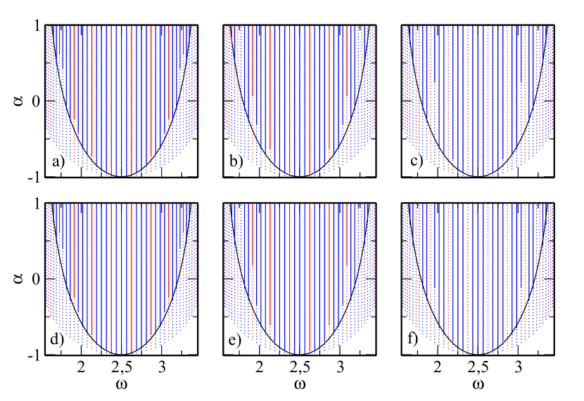
Figure 4: Bifurcation diagrams for different strengths $s$ of the shortcut in a ring of $N=100$ oscillators with a shortcut from node $\ell=26$ to node $N=100$; $\beta=2.5$. Dashed lines indicate unstable periodic orbits and solid lines stable periodic orbits. In black the stabilization line for $s=0$ is shown. The frequency of the solutions is plotted against the bifurcation parameter $\alpha$. The perturbation strength $s$ increases from left to right: a), d) $s=0.05$; b), e) $s=0.1$; c), f) $s=0.2$. The upper panels a), b), c) show the approximated diagram obtained from (32). The lower panels d), e), f) show results of numerical bifurcation analysis of the full system for comparison. These calculations were carried out with the program AUTO [27].

Resonances

An important observation for the perturbed system is that in comparison to the unperturbed case $s=0$, for small $s>0$ the point of stabilization of a periodic solution may be altered or not. It remains nearly the same if the corresponding eigenvalue $\lambda_{k}=\gamma_{N,k}+{\cal O}\left(s\right)$ fulfills

$$\arg\left(\gamma_{N,k}\right)\approx\arg\left(\gamma_{N,k}^{\ell}\right),$$ (33)

or equivalently, $\frac{k\left(l-1\right)}{N}\in\mathbb{Z}$. This corresponds to a situation where both components of the input $z_{1}\left(t\right)+sz_{\ell}\left(t\right)$ to node $z_{N}\left(t\right)$ possess approximately the same phase. At the same time it is a condition for maximizing the modulus $\left|\lambda_{k}\right|\approx\left|\gamma_{N,k}+\frac{s}{N}\gamma_{N,k}^{\ell}\right|$ and for $\gamma_{N,k}$ to span an eigenmode of both, the unperturbed cycle of length $N$ and of a cycle which has the same length $N-\ell-1$ as the newly created cycle $\ell\to N\to\left(N-1\right)\to...\to\ell$, i.e. to be an $N$-th and an $\left(N-\ell+1\right)$-th root of unity. On the contrary, the antiphase condition

$$\arg\left(\gamma_{N,k}\right)\approx\arg\left(\gamma_{N,k}^{\ell}\right)+\pi.$$ (34)

causes the point of stabilization to grow rapidly with increasing $s$, i.e., it destabilizes the corresponding periodic orbit. The more precisely the equality (34) holds, the more pronounced is the destabilizing effect of the additional link [see fig. 4].

4.2 Case II: Large $s$

For large $s$ both systems, the original (1) and the truncated (29), admit two types of periodic solutions emerging in bifurcations corresponding to eigenvalues of scale $\left|\lambda\right|\approx 0$ or $\left|\lambda\right|\approx s^{\nicefrac{{1}}{{N-\ell+1}}}$, respectively [see eq. (9), (10), and (30)]. In case of system (1) all these periodic solutions emerge in form of rotating eigenvectors (15)–(19) of the coupling matrix $G_{s}$ which leads to a locally pronounced activity in $z_{1}\left(t\right)$ for a corresponding eigenvalue $\left|\lambda\right|\approx 0$, and in $z_{N}\left(t\right)$ for $\left|\lambda\right|\approx s^{\nicefrac{{1}}{{N-\ell+1}}}$ [see fig. 3]. The same picture applies for bifurcations of (29) corresponding to the simple eigenvalues ($\left|\nu\right|\approx s^{\nicefrac{{1}}{{N-\ell+1}}}$) of $H_{s}$, while the $\ell-1$-fold bifurcation at $\alpha=0$ corresponding to $\nu=0$ simultaneously creates several solutions which are completely localized in the attached subsystem $\left(z_{1},...,z_{\ell-1}\right)$ where only the oscillators $z_{1},\,...,\,z_{k}$, $k=1,...,\ell-1$, are active and all others silent. For each of these solutions the first active element $z_{k}\left(t\right)=\sqrt{\alpha}e^{i\beta t}$ is located on the limit cycle of an isolated Stuart-Landau oscillator and all other $z_{j}$, $j<k$, lock either in phase or antiphase to their input signal $z_{j+1}$. However, these solutions can never stabilize, since the zero solution of the subsystem $z_{\ell},\,...,\,z_{N}$ is unstable after the first bifurcation corresponding to $\left|\nu\right|\approx s^{\nicefrac{{1}}{{n}}}$. Therefore, it suffices to study the inhomogeneous ring

$$\dot{z}_{j}\left(t\right) = \left(\mu-\left|z_{j}\left(t\right)\right|^{2}\right)z_{j}+z_{j+1}\left(t\right),\ j=1,...,n-1,$$

$$\dot{z}_{n}\left(t\right) = \left(\mu-\left|z_{n}\left(t\right)\right|^{2}\right)z_{n}+sz_{1}\left(t\right),\ n=N-\ell+1,$$ (35)

to understand the possibly stable dynamics of (29). To approximate the stability of the emerging periodic solutions one can proceed as for the case of small $s$: write the system in scaled rotating coordinates (20), linearize around the equilibrium solution (23), expand the variational equations in powers of $\varepsilon$ and truncate terms of order higher than ${\cal O}\left(\varepsilon\right)$.We obtain the following approximate variational equation [see Appendix E]:

$$\dot{\boldsymbol{x}}_{j} = -\left[s^{\frac{1}{n}}M_{\gamma_{n,k}}+\varepsilon\left(\left|v_{j}^{0}\left(s\right)\right|^{2}\left(\begin{array}[]{cc}3&0\\ 0&1\end{array}\right)-\left(\begin{array}[]{cc}1&0\\ 0&1\end{array}\right)\right)\right]\boldsymbol{x}_{j}$$ (43)

$$+\left[s^{\frac{1}{n}}M_{\gamma_{n,k}}+\varepsilon\left(\left|v_{j}^{0}\left(s\right)\right|^{2}-1\right)\left(\begin{array}[]{cc}1&0\\ 0&1\end{array}\right)\right]\boldsymbol{x}_{j+1},$$

where $\left|v_{j}^{0}\left(s\right)\right|^{2}=ns^{\frac{2(j-1)}{n}}\frac{s^{\frac{2}{n}}-1}{s^{2}-1}$. Although the loss of symmetry prevents us from applying an MSF approach, (43) enables us to approximate the Floquet exponents by solving numerically the characteristic equation of (43).

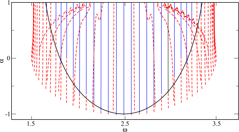
Figure 5: Bifurcation diagram for intermediate strength $s=5$ of the shortcut. Fixed parameters are $N=100$, $\ell=26$, $\beta=2.5$. Branches of unstable periodic orbits are indicated by dashed lines and stable branches by solid lines. Along the black line (13) the stabilization takes place for $s=0$. The frequency of the solutions is plotted against the bifurcation parameter $\alpha$. The calculations were carried out with the program AUTO [27].

5 Discussion

We have investigated how the introduction of a shortcut alters the dynamics in a unidirectional ring of Stuart-Landau oscillators. In absence of a shortcut, the system exhibits a bifurcation scenario similar to the Eckhaus instability observed in dissipative media. For small shortcut strengths $s$ we have found that the Eckhaus stabilization line is modulated in the following manner: The destabilizing impact on periodic solutions is stronger for non-resonant modes than for resonant ones. The latter correspond to wavenumbers that are compatible with the lengths of both cycles which exist in the perturbed system, i.e. for the cycle of length $N-\ell+1$ which contains the shortcut, as well as for the full cycle of length $N$. In contrary to the non-resonant solutions, the stabilization of the resonant periodic solutions occurs for similar parameter values as in the case without shortcut. As a result, one can control the destabilization of a specific set of wavenumbers via the link position $\ell$ and its strength $s$. In the case of a large shortcut strength $s$ we have provided an argument that the cycle of length $N-\ell+1$ dominates the dynamics and stable solutions can be treated as solutions of a single unidirectional inhomogeneous ring which has coupling strength $s$ at only one link.

Further investigations will be dedicated to how small perturbations may be used to select solutions with a specific wavenumber by adding a corresponding set of resonant links. More generally, our findings may help to understand how perturbations with a more complicated structure, consisting of several shortcuts, can influence the dynamics of a unidirectional ring. Moreover, our observations might even help to locate an unkown shortcut when one is only allowed to vary a bifurcation parameter and observe the dynamics, since the modulated Eckhaus line can be used to identify the shortcut. A strong shortcut can be used in arbitrary networks in order to localize the activity on the cycles in which they are contained and amplify the activity in particular on their targets.

Another point which was not investigated here but deserves a closer study is the development of profiles far from the bifurcation point. The simplest, most important phenomenon is that, for increasing $\alpha$, the exponential tails of the profiles develop into plateaus, where the profile amplitude is locally constant as a function of the component index. By taking the limit $N\to\infty$ one can argue that solutions may consist of several, sharply separated plateaus where each plateau can possess a different wavenumber. This complies with numerical observations, although all observed solutions with more than one plateau lie on the unstable branches which correspond to the inner spectral circle for large $s$. For sufficiently large values of $s$, those branches begin to curl with increasing $\alpha$ and seem to be unstable for arbitrary large values of $\alpha$ [see Fig. 5].

Appendix A Adjacency spectrum for large $s$

To apply the implicit function theorem and continue roots of the characteristic equation (7) for the case of large $s$, we define

$$F\left(\lambda,\tau,\vartheta\right)=\tau\lambda^{N}-\lambda^{\ell-1}-\vartheta.$$ (44)

Then $F\left(\lambda,\frac{1}{s},\frac{1}{s}\right)=0$ is equivalent to (7). We now apply the implicit function theorem twice to find the two distinct families (9) and (10) of small and large solutions of (7). Let us first compute

$$\partial_{\lambda}F\left(\lambda,\tau,\vartheta\right) = \tau N\lambda^{N-1}-\left(\ell-1\right)\lambda^{\ell-2},$$

$$\partial_{\tau}F\left(\lambda,\tau,\vartheta\right) = \lambda^{N},\qquad\partial_{\vartheta}F\left(\lambda,\tau,\vartheta\right)=-1.$$ (45)

Consider the equation

$$F\left(\lambda,0,\vartheta\right)=-\lambda^{\ell-1}-\vartheta=0.$$ (46)

It possesses $\ell-1$ solutions

$$\lambda_{1,k}\left(0,\vartheta\right)=\vartheta^{\frac{1}{\ell-1}}e^{i\frac{\pi}{\ell-1}}\gamma_{\ell-1,k},$$

$k=0,...,\ell-2$. Assuming (we show that below) that for $\left(\tau,\vartheta\right)\neq 0$ one can extend these solutions to smooth functions $\left(\tau,\vartheta\right)\mapsto\lambda_{1,k}\left(\tau,\vartheta\right)$ which solve $F\left(\lambda_{1,k}\left(\tau,\vartheta\right),\tau,\vartheta\right)=0$. These can be expanded in $\tau=0$ as

$$\lambda_{1,k}\left(\tau,\vartheta\right) = \lambda_{1,k}\left(0,\vartheta\right)-\partial_{\lambda}F\left(\lambda_{1,k}\left(0,\vartheta\right),0,\vartheta\right)^{-1}\partial_{\tau}F\left(\lambda_{1,k}\left(0,\vartheta\right),0,\vartheta\right)\tau+{\cal O}\left(\tau^{2}\right)$$

$$= \lambda_{1,k}\left(0,\vartheta\right)+\left(\left(\ell-1\right)\lambda_{1,k}^{\ell-2}\left(0,\vartheta\right)\right)^{-1}\lambda_{1,k}^{N}\left(0,\vartheta\right)\tau+{\cal O}\left(\tau^{2}\right)$$

$$= \lambda_{1,k}\left(0,\vartheta\right)+\frac{\lambda_{1,k}^{N-\ell+2}\left(0,\vartheta\right)}{\ell-1}\tau+{\cal O}\left(\tau^{2}\right)$$

and, for $\vartheta=\tau$,

$$\lambda_{1,k}\left(\tau,\tau\right)=\lambda_{1,k}\left(0,\tau\right)+\frac{\lambda_{1,k}^{N-\ell+2}\left(0,\tau\right)}{\ell-1}\tau+{\cal O}\left(\tau^{2}\right).$$ (47)

This gives a family of $\ell-1$ solutions of (7) situated near a small circle of radius $\sim\left(1/s\right)^{\frac{1}{\ell-1}}$. For $\tau\neq 0$ , the equation

$$F\left(\lambda,\tau,0\right)=\tau\lambda^{N}-\lambda^{\ell-1}=0$$ (48)

has an $\left(\ell-1\right)$-fold root at $\lambda=0$ which corresponds to the solutions of (46) and $N-\ell+1$ roots

$$\lambda_{2,k}\left(\tau,0\right)=\left|\tau\right|^{-\frac{1}{N-\ell+1}}\gamma_{N-\ell+1,k}$$ (49)

$k=0,...,N-\ell$. As before, we obtain an asymptotic representation

$$\lambda_{2,k}\left(\tau,\tau\right) = \lambda_{2,k}\left(\tau,0\right)-\partial_{\lambda}F\left(\lambda_{2,k}\left(\tau,0\right),\tau,0\right)^{-1}\partial_{\vartheta}F\left(\lambda_{2,k}\left(\tau,0\right),\tau,0\right)\tau+{\cal O}\left(\tau^{2}\right)$$ (50)

$$= \lambda_{2,k}\left(\tau,0\right)+\chi_{G_{s}}^{\prime}\left(\lambda_{2,k}\left(\tau,0\right)\right)^{-1}\tau+{\cal O}\left(\tau^{2}\right)$$

This is the family of solutions which lie near a larger circle of radius $\sim s^{\frac{1}{N-\ell+1}}$.

Now let us show that the interval of existence of the implicit functions $\tau\mapsto\lambda_{1,k}\left(\tau,\vartheta_{0}\right)$ and $\vartheta\mapsto\lambda_{2,k}\left(\tau_{0},\vartheta\right)$, respectively, indeed contain the points $\tau=\vartheta_{0}$ and $\vartheta=\tau_{0}$, respectively. Let us denote the implicit function in question simply $\lambda\left(\tau,\vartheta\right)$. If the implicit function theorem fails to provide an extension of $\lambda\left(\tau,\vartheta\right)$ in some point $\left(\tau_{\ast},\vartheta_{\ast}\right)>0$, we must have

$$\partial_{\lambda}F\left(\lambda_{\ast},\tau_{\ast},\vartheta_{\ast}\right)=\tau_{\ast}N\lambda_{\ast}^{N-1}-\left(\ell-1\right)\lambda_{\ast}^{\ell-2}=0$$ (51)

where $\lambda_{\ast}=\lambda\left(\tau_{\ast},\vartheta_{\ast}\right)$. Since $F\left(0,\tau,\vartheta\right)=0$ is equivalent to $\vartheta=0$, we may assume $\lambda_{\ast}\neq 0$. Thus, (51) is equivalent to

$$\lambda_{\ast}^{N-\ell+1}=\frac{\ell-1}{N\tau_{\ast}}.$$ (52)

Furthermore, from $(\ref{eq:large-s-function})=0$ we obtain $\tau_{\ast}=\lambda^{\ell-1-N}+\vartheta_{\ast}\lambda^{-N}$ which we insert into (51) to obtain

$$\lambda_{\ast}^{\ell-1}=-\frac{N}{N-\ell+1}\vartheta_{\ast}.$$ (53)

From (52) and (53), we obtain

$$\tau_{\ast}=\Gamma\left(\vartheta_{\ast}\right):=\frac{\ell-1}{N}\left(\frac{N-\ell+1}{N}\right)^{\frac{N-\ell+1}{\ell-1}}\vartheta_{\ast}^{-\frac{N-\ell+1}{\ell-1}}.$$

Since $\Gamma:\mathbb{R}_{>0}\to\mathbb{R}_{>0}$ is monotonic, we have

$$\partial_{\lambda}F\left(\lambda\left(\tau,\vartheta_{\ast}\right),\tau,\vartheta_{\ast}\right)\neq 0$$

for all $\tau<\tau_{\ast}=\Gamma\left(\vartheta_{\ast}\right)$. Since $\Gamma\left(\tau\right)\to\infty$, for $\tau\searrow 0$, there exists $\tau_{0}>0$ such that $\tau<\Gamma\left(\tau\right)$ and $\lambda\left(\tau,\tau\right)$ is defined uniquely, for $0<\tau<\tau_{0}$.

Appendix B Supercriticality of the Hopf bifurcations

To show that the bifurcations at $\alpha=-\Re\left(\lambda\right)$ of system (3) are supercritical for sufficiently large $s\geq 0$, we use the projection method for center manifolds [25]. In the following, we write the vector field of (3) as

$$f_{\alpha}\left(\boldsymbol{z}\right)=A\boldsymbol{z}+\frac{1}{6}C\left(\boldsymbol{z},\boldsymbol{z},\boldsymbol{z}\right),$$

where $A=\mathrm{Id}_{N}\otimes M_{\mu}+G_{s}\otimes\mathrm{Id}_{2}$ is the linearization of $f_{\alpha}$ at $\boldsymbol{z}=0$ and the trilinear function $C$ contains all cubic terms. Furthermore, let $\boldsymbol{v}\in\mathbb{R}^{2N}$ be an eigenvector of $A$ corresponding to the eigenvalue $\mu+\lambda$, $\lambda\in\sigma(G_{s})$. (The case of an eigenvalue $\bar{\mu}+\lambda$ can be treated analogously.) Let $w\in\mathbb{R}^{2N}$ be the normalized adjoint eigenvector corresponding to $\boldsymbol{v}$, i.e. $A^{T}\boldsymbol{w}=(\bar{\mu}+\bar{\lambda})\boldsymbol{w}$ and $\left\langle\boldsymbol{w},\boldsymbol{v}\right\rangle=1$. We have

$$\boldsymbol{v} = \left(1,\lambda,...,\lambda^{N-1}\right)^{T}\otimes\left(i,1\right)^{T},$$ (54)

$$\boldsymbol{w} = \frac{1}{\bar{\kappa}}\left(\overline{\lambda}{}^{\ell-1},...,\overline{\lambda},\overline{\lambda}^{N},...,\overline{\lambda}^{\ell}\right)^{T}\otimes\left(i,1\right)^{T},$$ (55)

with $\kappa=2\lambda^{\ell-1}(\left(\ell-1\right)+\left(N-\ell+1\right)\lambda^{N})$. A Hopf bifurcation at $\alpha$ is supercritical for a negative and subcritical for a positive first Lyapunov coefficient

$$l_{1}\left(0\right)=\frac{1}{2\omega_{0}^{2}}\Re\left(\left\langle\boldsymbol{w},C\left(\boldsymbol{v},\boldsymbol{v},\overline{\boldsymbol{v}}\right)\right\rangle\right),$$ (56)

where $\omega_{0}=\beta+\Im\left(\lambda\right)\neq 0$. Writing $C=(C_{1,1},C_{1,2},\dots,C_{N,1},C_{N,2})$ we obtain

$$C_{j,1}\left(\boldsymbol{v},\boldsymbol{v},\overline{\boldsymbol{v}}\right)=-6v_{j,1}\left|v_{j,1}\right|^{2}-2\left(2v_{j,1}\left|v_{j,2}\right|^{2}+v_{j,2}^{2}\overline{v}_{j,1}\right)=iC_{j,2}\left(\boldsymbol{v},\boldsymbol{v},\overline{\boldsymbol{v}}\right),$$ (57)

for $1\leq j\leq N$. Using this, we get

$$\left\langle\boldsymbol{w},C\left(\boldsymbol{v},\boldsymbol{v},\overline{\boldsymbol{v}}\right)\right\rangle=-8\left(\frac{\sum_{j=1}^{\ell-1}\left|\lambda\right|^{2\left(j-1\right)}+\lambda^{N}\sum_{j=\ell}^{N}\left|\lambda\right|^{2\left(j-1\right)}}{\left(\ell-1\right)+\left(N-\ell+1\right)\lambda^{N}}\right)$$ (58)

For large $s>0$ we distinguish two cases.For the case $\left|\lambda\right|\sim s^{\nicefrac{{1}}{{N-\ell+1}}}$, we find that

$$\Re\left(\left\langle\boldsymbol{w},C\left(\boldsymbol{v},\boldsymbol{v},\overline{\boldsymbol{v}}\right)\right\rangle\right)\to-\infty,\ \text{as }s\to\infty,$$

and for the case $\left|\lambda\right|\sim s^{-\nicefrac{{1}}{{\ell-1}}}$,

$$\Re\left(\left\langle\boldsymbol{w},C\left(\boldsymbol{v},\boldsymbol{v},\overline{\boldsymbol{v}}\right)\right\rangle\right)\nearrow 0,\ \text{as }s\to\infty.$$

This means that for sufficiently large $s$, we have $l_{1}\left(0\right)<0$ for all eigenvalues. Thus, all bifurcations are supercritical.

Appendix C Supercriticality for an inhomogeneous ring

Consider the case $\ell=1$ and $s$ arbitrary, i.e. a ring with inhomogeneous coupling strengths. Here, using (58) and the characteristic equation, $\lambda^{N}=1+s$, we get

$$\left\langle\boldsymbol{w},C\left(\boldsymbol{v},\boldsymbol{v},\overline{\boldsymbol{v}}\right)\right\rangle = -\frac{8\left(1-\left(1+s\right)^{2}\right)}{N\left(1-\left|1+s\right|^{2/N}\right)}.$$ (59)

Thus, in the case of the inhomogeneous ring the bifurcation is supercritical for arbitrary $s$.

Appendix D Expansion of the solution profiles for small perturbations

The linearization of (21)–(22) at (23) is

$$0 = \left(\alpha+i\left(\beta-\omega\right)-\varepsilon\left|v_{j}\right|^{2}\right)+\frac{v_{j+1}}{v_{j}},$$ (60)

$$0 = \left(\alpha+i\left(\beta-\omega\right)-\varepsilon\left|v_{N}\right|^{2}\right)+\frac{v_{1}}{v_{N}}+s\frac{v_{\ell}}{v_{N}},$$

From these equations we will now find expressions for the first terms of the Taylor expansions of the unknown functions

$$\omega_{k}\left(\varepsilon,s\right)=\omega_{00}+\varepsilon\omega_{10}+s\omega_{11}+{\cal O}\left(\left(\left|\varepsilon\right|+\left|s\right|\right)^{2}\right)$$

and

$$v_{j}\left(\varepsilon,s\right)=v_{j}^{00}+\varepsilon v_{j}^{10}+sv_{j}^{01}+{\cal O}\left(\left(\left|\varepsilon\right|+\left|s\right|\right)^{2}\right),\ j=1,...,N.$$

Terms at order ${\cal O}\left(1\right)$

Considering the terms in $s=\varepsilon=0$ in (60) yields the circular equations (let $v_{N+1}^{00}:=v_{1}^{00}$)

$$0 = \alpha^{0}+i(\beta-\omega_{00})+\frac{v_{j+1}^{00}}{v_{j}^{00}},$$ (61)

with the shorthand $\alpha^{0}=\alpha_{k}\left(0\right)=-\cos\left(2\pi k/N\right)$. This leads to

$$\left(-\alpha^{0}-i\left(\beta-\omega_{00}\right)\right)^{N}=1$$

which contains no new information, since it only determines $\alpha^{0}=-\Re\left(\lambda_{0}\right)$ and $\omega_{00}=\beta+\Im\left(\lambda_{0}\right)$ with an $N$-th root of unity

$$\lambda_{0}=\lambda_{k}\left(0\right)=e^{i\frac{2\pi k}{N}}.$$

For the profile, (61) yields

$$v_{j+1}^{00}=\lambda_{0}^{j}r_{0},$$ (62)

with a hitherto unknown scale factor $r_{0}:=v_{1}^{00}$. Without loss of generality, one may choose $v_{1}\left(\varepsilon,s\right)\in\mathbb{R}_{\geq 0}$, because of the phase shift invariance of (15). In particular, we then have $r_{0}\in\mathbb{R}_{+}$.

Terms at order ${\cal O}\left(\varepsilon\right)$

At first order in $\varepsilon$ we obtain another set of circular equations (let again $v_{N+1}^{10}=v_{1}^{10}$)

$$0 = 1-i\omega_{10}-r_{0}^{2}+\frac{\lambda_{0}}{r_{0}}\left(\frac{v_{j+1}^{10}}{\lambda_{0}^{j}}-\frac{v_{j}^{10}}{\lambda_{0}^{j-1}}\right)$$

which leads us to the following recursion

$$\frac{v_{j+1}^{10}}{\lambda_{0}^{j}}=\left(r_{0}^{2}-\left(1-i\omega_{10}\right)\right)\frac{r_{0}}{\lambda_{0}}+\frac{v_{j}^{10}}{\lambda_{0}^{j-1}}$$ (63)

Defining $a_{j}=\frac{v_{j}^{10}}{\lambda_{0}^{j-1}}$ and $A=\left(r_{0}^{2}-(1-i\omega_{10})\right)\frac{r_{0}}{\lambda_{0}}$, equation (63) can be written as $a_{j+1}=A+a_{j}$ with the solution $a_{j+1}=jA+a_{1}$. Because of the circularity $a_{N+1}=a_{1}$ we then have $a_{1}=NA+a_{1}$ which determines $A=0$. Therefore, $r_{0}^{2}=(1-i\omega_{10})$ and finally

$$\omega_{10}=0\ \text{and}\ r_{0}=1$$ (64)

That means at first order the frequency of the oscillations does not depend on $\varepsilon$. For the profiles $v_{j}^{10}$ it follows (as at order ${\cal O}\left(1\right)$)

$$v_{j+1}^{10}=\lambda_{0}^{j}r_{1\text{0}},$$ (65)

with $r_{10}:=v_{1}^{10}\in\mathbb{R}$.

Terms at $O\left(s\right)$

Due to the fact that $s$ perturbs the network symmetry, the equations at order ${\cal O}\left(s\right)$ are more complex than those at order ${\cal O}\left(\varepsilon\right)$. Again, the linear terms in $s$ of (60) give a recursive formula

$$\frac{v_{j+1}^{01}}{\lambda_{0}^{j}} = \frac{1}{\lambda_{0}}\left(i\omega_{01}-\alpha^{1}\right)+\frac{v_{j}^{01}}{\lambda_{0}^{j-1}},$$

$$v_{1}^{01} = \frac{1}{\lambda_{0}}\left(i\omega_{01}-\alpha^{1}\right)-\lambda_{0}^{\ell-1}+\frac{v_{N}^{01}}{\lambda_{0}^{N-1}},$$ (66)

where $\alpha^{1}=-\frac{d}{ds}\Re\left(\lambda_{k}\left(s\right)\right)\mid_{s=0}$. For $j<N$ we have $\frac{v_{j+1}^{01}}{\lambda_{0}^{j}}=\frac{j}{\lambda_{0}}\left(i\omega_{01}-\alpha^{1}\right)+v_{1}^{01}$. Inserting the resulting expression for $v_{N}^{01}$ in the second equation gives $v_{1}^{01}=\frac{N}{\lambda_{0}}\left(i\omega_{01}-\alpha^{1}\right)-\lambda_{0}^{\ell-1}+v_{1}^{01}$. Therefore, $N\left(i\omega_{01}-\alpha^{1}\right)=\lambda_{0}^{\ell}$ or equivalently

$$\omega_{01}=\frac{1}{N}\Im\left(\lambda_{0}^{\ell}\right)\ \text{and}\ \alpha^{1}=-\frac{1}{N}\Re\left(\lambda_{0}^{\ell}\right).$$ (67)

The perturbations $v_{j+1}^{01}$ of the profile are then determined as

$$v_{j+1}^{01} = \left(\frac{j}{N}\lambda_{0}^{\ell-1}+r_{01}\right)\lambda_{0}^{j}.$$ (68)

up to a scaling $r_{01}:=v_{1}^{01}\in\mathbb{R}$ as above.

Higher order terms

To determine the amplitudes $r_{10}$ and $r_{01}$ of the perturbations $v_{j}^{10}$ and $v_{j}^{01}$, $j=1,...,N$, we need to calculate the second order terms ${\cal O}\left(\varepsilon^{2}\right)$, ${\cal O}\left(s^{2}\right)$, and ${\cal O}\left(\varepsilon\cdot s\right)$ of (60) due to the nonlinear term. We omit this here and just give the resulting values

$$r_{10}=0\ \text{and}\ r_{01}=0.$$ (69)

The vanishing $r_{10}$ means that at first order the profiles do not depend on $\varepsilon$.

Appendix E Expansion of the solution profiles for the inhomogeneous ring

A periodic solution of (35) corresponds to a fixed point in co-rotating coordinates (20). The stability of this fixed point is governed by its variational equations

$$\dot{\boldsymbol{x}}_{j} = \left(M_{\alpha+i\left(\beta-\omega\right)}-\varepsilon\left(s\right)\left|v_{j}\right|^{2}\left[\begin{matrix}3&0\\ 0&1\end{matrix}\right]\right)\dot{\boldsymbol{x}}_{j}+M_{\frac{v_{j+1}}{v_{j}}}\dot{\boldsymbol{x}}_{j+1},$$ (70)

$$\dot{\boldsymbol{x}}_{n} = \left(M_{\alpha+i\left(\beta-\omega\right)}-\varepsilon\left(s\right)\left|v_{n}\right|^{2}\left[\begin{matrix}3&0\\ 0&1\end{matrix}\right]\right)\dot{\boldsymbol{x}}_{n}+sM_{\frac{v_{1}}{v_{n}}}\dot{\boldsymbol{x}}_{1},$$ (71)

Higher order terms of $\omega=\omega\left(\varepsilon,s\right)$ and $v_{j}=v_{j}\left(\varepsilon,s\right)$ can be determined by the equations

$$0 = \left(\alpha+i\left(\beta-\omega\right)\right)-\varepsilon\left|v_{j}\right|^{2}+\frac{v_{j+1}}{v_{j}},$$ (72)

$$0 = \left(\alpha+i\left(\beta-\omega\right)\right)-\varepsilon\left|v_{n}\right|^{2}+s\frac{v_{1}}{v_{n}},$$ (73)

which are obtained from inserting the solution ansatz (15) into (35). Solving for real and imaginary parts yields the conditions

$$\omega-\beta = \Im\left(\frac{v_{j+1}}{v_{j}}\right)=s\Im\left(\frac{v_{1}}{v_{n}}\right),$$ (74)

$$\alpha = \varepsilon\left|v_{j}\right|^{2}-\Re\left(\frac{v_{j+1}}{v_{j}}\right)=\varepsilon\left|v_{n}\right|^{2}-s\Re\left(\frac{v_{1}}{v_{n}}\right).$$ (75)

Note that we expand the unknown functions only in $\varepsilon$, keeping $s$ arbitrary. Using (74) and (75) the variational equations (70)–(71) write

$$\dot{\boldsymbol{x}}_{j} = -\left[M_{\frac{v_{j+1}}{v_{j}}}+2\varepsilon\mid v_{j}\mid^{2}\left(\begin{array}[]{cc}1&0\\ 0&0\end{array}\right)\right]\boldsymbol{x}_{j}+M_{\frac{v_{j+1}}{v_{j}}}\boldsymbol{x}_{j+1},$$ (78)

$$\dot{\boldsymbol{x}}_{n} = -\left[sM_{\frac{v_{1}}{v_{n}}}+2\varepsilon\mid v_{n}\mid^{2}\left(\begin{array}[]{cc}1&0\\ 0&0\end{array}\right)\right]\boldsymbol{x}_{n}+sM_{\frac{v_{1}}{v_{n}}}\boldsymbol{x}_{1}.$$ (81)

In the rest of this section, we find expressions for $\frac{v_{j+1}}{v_{j}}\left(0,s\right)$ and $\frac{\partial}{\partial\varepsilon}\left[\frac{v_{j+1}}{v_{j}}\left(\varepsilon,s\right)\right]_{|\varepsilon=0}$ which can be inserted into (78)–(81) to obtain (43). Let

$$\omega\left(\varepsilon,s\right)=\omega_{0}\left(s\right)+\varepsilon\omega_{1}\left(s\right)+{\cal O}\left(\varepsilon^{2}\right)$$

and

$$v_{j}\left(\varepsilon,s\right)=v_{j}^{0}\left(s\right)+\varepsilon v_{j}^{1}\left(s\right)+{\cal O}\left(\varepsilon^{2}\right),\ j=1,...,N.$$

For $\varepsilon=0$, equations (72)–(73) yield

$$v_{j+1}^{0} = \left(i\left(\omega_{0}-\beta\right)-\alpha_{0}\right)v_{j}^{0}=...=\left(i(\omega_{0}-\beta)-\alpha_{0}\right)^{j}v_{1}^{0},$$

$$v_{1}^{0} = \frac{1}{s}\left(i\left(\omega_{0}-\beta\right)-\alpha_{0}\right)v_{n}^{0},$$

where $\alpha_{0}=-\Re\left(\lambda_{k}\left(s\right)\right)=-s^{\nicefrac{{1}}{{n}}}\cos\left(2\pi k/n\right)$ is the critical value at which the periodic solution emerges, $\omega_{0}=\beta+\Im\left(\lambda_{k}\right)$ is the initial frequency, and the initial profile is given by $v_{j}^{0}=\lambda_{k}^{j-1}v_{1}^{0}$.

For terms of order ${\cal O}\left(\varepsilon\right)$ one obtains

$$\omega_{1}=0,\ \left|v_{1}^{0}\right|^{2}=n\frac{s^{\frac{2}{n}}-1}{s^{2}-1},\ \text{and }v_{j}^{1}=v_{j}^{0}\sum_{l=0}^{j-1}\left(|v_{j-l}^{0}|^{2}-1\right)+\lambda_{k}^{j}v_{1}^{1}$$

To approximate (78)–(81), we calculate the first order terms of the quotients $v_{j+1}/v_{j}$, which gives at ${\cal O}(\varepsilon^{0})$

$$\frac{v_{j+1}^{0}}{v_{j}^{0}}=s^{\nicefrac{{1}}{{n}}}\gamma_{n,k},$$

and at ${\cal O}(\varepsilon)$

$$\left(\frac{v_{j+1}}{v_{j}}\right)^{1} = \left|v_{j}^{0}\right|^{2}-1.$$

References

- [1] S. Boccaletti, V. Latora, Y. Moreno, M. Chavez, and D.-U. Hwanga. Complex networks: Structure and dynamics. Physics Reports, 424:175–308, 2006.
- [2] A. Koseska and J. Kurths. Topological structures enhance the presence of dynamical regimes in synthetic networks. Chaos: An Interdisciplinary Journal of Nonlinear Science, 20(4):045111, 2010.
- [3] Juan G. Restrepo, Edward Ott, and Brian R. Hunt. Spatial patterns of desynchronization bursts in networks. Physical Review E, 69(6):066215, 2004.
- [4] A. Takamatsu, R. Tanaka, H. Yamada, T. Nakagaki, T. Fujii, and I. Endo. Spatiotemporal symmetry in rings of coupled biological oscillators of physarum plasmodial slime mold. Physical Review Letters, 87(7):078102, July 2001.
- [5] R. Milo, S. Shen-Orr, S. Itzkovitz, N. Kashtan, D. Chklovskii, and U. Alon. Network motifs: Simple building blocks of complex networks. Science, 298(5594):824–827, 2002.
- [6] D. M. Abrams and S. H. Strogatz. Chimera states for coupled oscillators. Physical Review Letters, 93(17):174102, 2004.
- [7] H. Daido. Strange waves in coupled-oscillator arrays: Mapping approach. Physical Review Letters, 78(9):1683–1686, 1997.
- [8] Juan G. Restrepo, Edward Ott, and Brian R. Hunt. Desynchronization waves and localized instabilities in oscillator arrays. Physical Review Letters, 93(11):114101, 2004.
- [9] I. Waller and R. Kapral. Spatial and temporal structure in systems of coupled nonlinear oscillators. Physical Review A, 30(4):2047–2055, 1984.
- [10] Wei Zou and Meng Zhan. Splay states in a ring of coupled oscillators: From local to global coupling. SIAM Journal on Applied Dynamical Systems, 8:1324–1340, 2009.
- [11] Y. Horikawa and H. Kitajima. Transient chaotic rotating waves in a ring of unidirectionally coupled symmetric bonhoeffer-van der pol oscillators near a codimension-two bifurcation point. Chaos, 22(3):033115, 2012.
- [12] Yo Horikawa. Exponential dispersion relation and its effects on unstable propagating pulses in unidirectionally coupled symmetric bistable elements. Communications in Nonlinear Science and Numerical Simulation, 17(7):2791–2803, 2012.
- [13] P. Perlikowski, S. Yanchuk, M. Wolfrum, A. Stefanski, P. Mosiolek, and T. Kapitaniak. Routes to complex dynamics in a ring of unidirectionally coupled systems. Chaos, 20:013111, 2010.
- [14] S. Yanchuk and M. Wolfrum. Destabilization patterns in chains of coupled oscillators. Physical Review E, 77(2):026212, 2008.
- [15] O. V. Popovych, S. Yanchuk, and P. A. Tass. Delay- and coupling-induced firing patterns in oscillatory neural loops. Physical Review Letters, 107:228102, 2011.
- [16] P. Perlikowski, S. Yanchuk, O. V. Popovych, and P. A. Tass. Periodic patterns in a ring of delay-coupled oscillators. Physical Review E, 82(3):036208, September 2010.
- [17] P. C. Bressloff, S. Coombes, and B. de Souza. Dynamics of a ring of pulse-coupled oscillators: Group-theoretic approach. Physical Review Letters, 79(15):2791–2794, 1997.
- [18] J.J. Collins and I. Stewart. A group-theoretic approach to rings of coupled biological oscillators. Biological Cybernetics, 71(2):95–103, 1994.
- [19] N. Strelkowa and M. Barahona. Transient dynamics around unstable periodic orbits in the generalized repressilator model. Chaos, 21(2):023104, 2011.
- [20] A. Vishwanathan, G. Bi, and H.C. Zeringue. Ring-shaped neuronal networks: a platform to study persistent activity. Lab on a Chip, 11(6):1081–8, 2011.
- [21] Guy Van der Sande, Miguel C. Soriano, Ingo Fischer, and Claudio R. Mirasso. Dynamics, correlation scaling, and synchronization behavior in rings of delay-coupled oscillators. Physical Review E, 77:055202, 2008.
- [22] Wiktor Eckhaus. Studies in Non-Linear Stability Theory, volume 6 of Springer Tracts in Natural Philosophy. Springer, New York, 1965.
- [23] Laurette S. Tuckerman and Dwight Barkley. Bifurcation analysis of the Eckhaus instability. Physica D, 46:57–86, 1990.
- [24] Louis M. Pecora and Thomas L. Carroll. Master stability functions for synchronized coupled systems. Physical Review Letters, 80:2109–2112, 1998.
- [25] Yuri Kuznetsov. Elements of Applied Bifurcation Theory, volume 112 of Applied Mathematical Sciences. Springer-Verlag, 1995.
- [26] N. Fenichel. Persistence and smoothness of invariant manifolds for flows. Indiana University Mathematics Journal, 21(193-226):1972, 1971.
- [27] Eusebius J. Doedel. AUTO-07P: Continuation and bifurcation software for ordinary differential equations. Montreal, Canada, April 2006.