The BOSS-WiggleZ overlap region II: dependence of cosmic growth on galaxy type

Abstract

The anisotropic galaxy 2-point correlation function (2PCF) allows measurement of the growth of large-scale structures from the effect of peculiar velocities on the clustering pattern. We present new measurements of the auto- and cross- correlation function multipoles of 69,180 WiggleZ and 46,380 BOSS-CMASS galaxies sharing an overlapping volume of $\sim 0.2$ $(h^{-1}$Gpc)³. Analysing the redshift-space distortions (RSD) of galaxy 2-point statistics for these two galaxy tracers, we test for systematic errors in the modelling depending on galaxy type and investigate potential improvements in cosmological constraints. We build a large number of mock galaxy catalogs to examine the limits of different RSD models in terms of fitting scales and galaxy type, and to study the covariance of the measurements when performing joint fits. For the galaxy data, fitting the monopole and quadrupole of the WiggleZ 2PCF on scales $24<s<80$ $h^{-1}$Mpc produces a measurement of the normalised growth rate $f\sigma_{8}(z=0.54)=0.409\pm 0.059$, whereas for the CMASS galaxies we found a consistent constraint of $f\sigma_{8}(z=0.54)=0.466\pm 0.074$, When combining the measurements, accounting for the correlation between the two surveys, we obtain $f\sigma_{8}(z=0.54)=0.413\pm 0.054$, in agreement with the $\Lambda$CDM-GR model of structure growth and with other survey measurements.

1 Introduction

The evolution of the spatial distribution of galaxies on large scales is deeply influenced by the physics of gravitational attraction, cosmic expansion, and the conditions of the early Universe, and constitutes an important probe and discriminator of cosmological models. Spectroscopic galaxy surveys map this distribution using the distance-redshift relation, but due to peculiar velocities induced by the gravitational field, these maps also contain ‘redshift-space distortions’ (RSD) of the spatial positions of the galaxies, which modify the true (i.e. real space) pattern of the spatial clustering of galaxies. Kaiser (1987) showed that on large scales the peculiar velocity field ${\bf v}$ (in dimensionless units of the Hubble velocity) is related to the matter overdensity $\delta_{m}$ as $\nabla\cdot{\bf v}=-f\delta_{m}$, where the proportionality parameter $f(z)$ is called the linear growth rate of structure. Modelling the redshift-space clustering, in consequence, allows us to constrain cosmological parameters through estimations of $f(z)$. Using Kaiser’s findings, the pioneering works in the 2dFGRS survey (Peacock et al., 2001; Hawkins et al., 2003) in the local $z\sim 0.1$ Universe, measured the redshift-space two-point clustering of galaxies, which resulted in a confirmation of the concordance $\Lambda$CDM model at present times. With the advent of galaxy surveys at higher redshifts, we can now trace the history of $f(z)$ and obtain constraints on cosmological models and the nature of dark energy (Linder & Cahn, 2007).

However, important challenges must be addressed before we can use this tool effectively. On the observational side, the most important factors limiting the statistical precision of the clustering measurements obtained from different surveys are the limited volume that the surveys can map, due to the sample variance from fluctuations in the clustering on different regions of the universe, and the discreteness of the galaxy field known as shot noise (e.g. Kaiser, 1986; White et al., 2009)

In addition, large-scale structures are subject to a variety of systematic non-linear effects which affect our capacity to model the signal, particularly on small scales. First, we have non-linear growth of structure, such that even on large scales, the Kaiser relations are insufficient to account for the measured clustering in galaxy data and simulations. Peacock (1992), and more recently Scoccimarro (2004); Taruya et al. (2010); Seljak & McDonald (2011); Wang et al. (2013), among others, have improved the basic ‘Kaiser’ model by including various non-linear effects in the matter clustering. Second, there is scale-dependent complexity in how galaxies trace haloes and cross-correlate to matter, known as galaxy bias. Third, galaxies possess non-linear pairwise velocities on small scales. The latest attempts to use the 2-point clustering pattern to model RSD have taken these and other effects into account (e.g. Reid et al., 2012; Beutler et al., 2012; Sánchez et al., 2013; de la Torre et al., 2013; Contreras et al., 2013; Beutler et al., 2014, as recent examples), allowing us to confront predictions from different cosmological models.

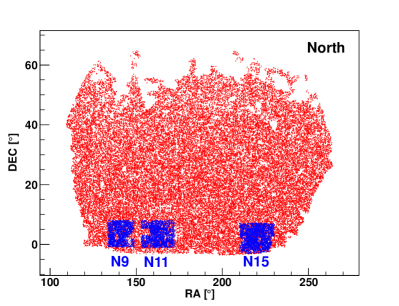
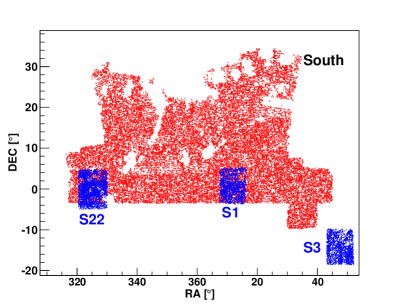
Figure 1: Sky coverage of BOSS-CMASS DR11 (red) and WiggleZ (blue). The left panel shows the northern part of the surveys, while the right panel shows the southern sky coverage. Five of the six WiggleZ regions are covered by CMASS, with a total of 69,180 WiggleZ galaxies and 46,380 CMASS galaxies in the overlap volume.

Although in linear theory all galaxies respond as test particles to the gravitational field, in detail the non-linear systematics depend on tracers themselves. This is because galaxy formation is affected by many non-linear processes such as small-scale dynamics of halo formation, environment, and complex baryonic processes determining the luminosity and colour at a given time, which are the main observables when selecting galaxies for a large-scale survey. Therefore, the analysis and modelling of two overlapping tracers makes it possible to constrain details of the clustering and formation of the galaxy tracers themselves. Previous work has focused on cross-correlating a tracer with well known properties with a second tracer we wish to study (e.g. Martínez et al., 1999; Chen, 2009; Mountrichas et al., 2009; Font-Ribera et al., 2013). In our current study we approach this in a cosmological context, in which a comparison of results using different tracers in the same volume tests for systematic errors in modelling of bias and redshift-space distortions.

In this work we present measurements and analysis of RSD using galaxies from the WiggleZ Dark Energy Survey (Drinkwater et al., 2010) and the CMASS galaxy sample from the Baryon Oscillation Spectroscopic Survey (BOSS, Eisenstein et al., 2011). At a redshift of $z\approx 0.6$, the WiggleZ team targeted Emission Line Galaxies hosted in low-to-intermediate mass halos, which have low bias ($b_{\rm WiggleZ}\sim 1$, see Blake et al., 2011b; Contreras et al., 2013; Marín et al., 2013), while the CMASS sample consists of luminous, mostly red galaxies with $b_{\rm CMASS}\sim 2$ (Reid et al., 2012; Tojeiro et al., 2012; Chuang et al., 2013; Kazin et al., 2013) with similar number density $n\sim 2-3\times 10^{-4}$ ($h^{-1}$Mpc)^-3. With an overlap volume of approximately 0.2 ($h^{-1}$Mpc)^-3, this is, to date, the largest volume overlapping sample between two different galaxy redshift surveys. We measure the redshift-space auto- and cross- correlation functions of these galaxies and explore the constraints on the cosmic growth rate using the two tracers. Our work is supported by a large suite of mock catalogs, which we generated by performing abbreviated N-body methods (COLA, Tassev et al., 2013) to model potential systematics coming from observational issues, test different RSD models and their regime of validity, and determine covariances.

A potential advantage of a multi-tracer analysis was described by McDonald & Seljak (2009), who noted that the correlations in an overlapping volume, if the number density of the tracers is large, can be used to reduce the sample variance error and improve the measurements of the growth rate. After this initial work, different applications of the multitracer method have been explored by various authors, using different observables such as photometric redshift surveys, weak lensing, gravitational redshifts, signatures of first stars and constraints on primordial non-gaussianity and modified gravity (Seljak, 2009; Bernstein & Cai, 2011; Gaztañaga et al., 2012; Asorey et al., 2013; Croft, 2013; Yoo & Seljak, 2013; Lombriser et al., 2013). Blake et al. (2013) applied this method to the GAMA survey, producing modest gains from the multitracer method, up to 20% in the constraints of $f$ at two different epochs, $z=0.18$ and $z=0.38$. Ross et al. (2014) measured the clustering of BOSS galaxies as a function of their colour and did not detect significant differences in distance scale or structure growth measurements. Although the datasets used in our study are too sparse to expect large improvement, we include this effect by computing the full covariance of the measurements using our mock galaxy catalogs.

We present in section $\S$2 the surveys used in our study. In $\S$3 we present the methods and results of the auto- and cross- correlation between tracers. In $\S$4 we show models of the RSD and constraints in the model parameters and the growth rate at $z=0.54$. Finally in $\S$5 we summarize our results and conclude. This is the second work of a series of papers analysing clustering in the BOSS-WiggleZ overlap region. Paper I (Beutler et al., 2015) focuses on the analysis of the Baryonic Acoustic Oscillation signal of these two tracers in the common volume.

For clarity we will use the name ‘CMASS-BW’ and ‘WiggleZ-BW’ for the CMASS and WiggleZ samples limited to the overlap region between the two surveys. We assume a fiducial flat $\Lambda$CDM cosmological model as defined in Komatsu et al. (2009), where the matter density is $\Omega_{\rm{m}}=0.273$, baryon density of $\Omega_{\rm{b}}$ = 0.045, a spectral index of $n_{s}$ = 0.963, an r.m.s. of density fluctuations averaged in spheres of radii at 8 $h^{-1}$Mpc of $\sigma_{8}$ = 0.81 and $h=0.71$. The Hubble rate at redshift $z$=0 is $H_{0}$= 100$h$ km s^-1 Mpc^-1 is adopted to convert redshifts to distances, which are measured in $h^{-1}$Mpc.

2 Data & Mock catalogs

2.1 The WiggleZ survey

The WiggleZ Dark Energy Survey (Drinkwater et al., 2010) is a large-scale galaxy redshift survey performed over 276 nights with the AAOmega spectrograph (Sharp et al., 2006) on the 3.9m Anglo-Australian Telescope. With a area coverage of 816 deg², this survey has mapped $207,000$ bright emission-line galaxies over a redshift range $0.1<z<1.0$. Target galaxies in six different regions were chosen using UV photometric data from the GALEX survey (Martin et al., 2005) matched with optical photometry from the Sloan Digital Sky Survey (SDSS DR4, Adelman-McCarthy et al. 2006) and from the Red-Sequence Cluster Survey 2 (RCS2, Gilbank et al. 2011). The selection criteria consisted of applying magnitude and colour cuts (Drinkwater et al., 2010) in order to select star-forming galaxies with bright emission lines with a redshift distribution centered around $z\sim 0.6$. The selected galaxies were observed in 1-hour exposures using the AAOmega spectrograph, and their redshifts were estimated from strong emission lines. The number density of WiggleZ galaxies averages $\sim 3\times 10^{-4}$ $(h^{-1}$Mpc)^-3 at $z=0.6$.

2.2 The CMASS Sample

The Baryon Oscillation Spectroscopic Survey of the Sloan Digital Sky Survey III (SDSS-III, Eisenstein et al., 2011; Dawson et al., 2013), which is now complete, was designed to obtain spectra and redshifts for 1.35 million bright galaxies over a footprint $\sim$ 10,000 deg². These galaxies are selected from the SDSS-III imaging and have been observed together with 160,000 quasars and 100,000 ancillary targets (Gunn et al., 2006; Bolton et al., 2012; Smee et al., 2013). The CMASS sample is composed of luminous, mostly red galaxies selected to probe large-scale structure at intermediate redshifts, achieving a number density of $\sim 3\times 10^{-4}$ $(h^{-1}$Mpc)^-3. The DR11 catalog (Alam et al., 2015) includes 1,100,000 spectra out of which the CMASS sample contains $\approx$ 550,000 galaxies in the redshift range $0.43<z<0.7$.

Table 1: Overlapping samples analysed in this study.

Region	WiggleZ-BW	WiggleZ-BW	CMASS-BW	CMASS-BW	Cross-pairs
	$N_{gal}$	$z_{avg}$	$N_{gal}$	$z_{avg}$	$z_{avg}$
S01	6620	0.61	5720	0.53	0.57
N09	13940	0.56	9360	0.53	0.54
N11	15560	0.55	10580	0.53	0.54
N15	22740	0.56	14660	0.54	0.54
S22	10320	0.55	6060	0.53	0.54
Total	69180	0.56	46380	0.53	0.54

2.3 Overlap volumes

We define the overlap regions between CMASS and WiggleZ using the random galaxy catalogs generated for each survey, gridding the sky into 0.1 deg² regions and selecting cells containing both CMASS and WiggleZ random points. As seen in Figure 1, five of the six WiggleZ regions have considerable overlap with CMASS galaxies, totalling 560 deg² and a volume of 0.218 ($h^{-1}$Gpc)³ in the $0.43<z<0.7$ range. This results in an overlap sample of 69,180 WiggleZ galaxies and 46,380 CMASS galaxies.

Figure 2 shows the redshift distribution of the two samples in the different regions, which is similar in the range $0.5<z<0.6$; outside that range the CMASS galaxy counts rapidly decline. To estimate how these differences will affect our results, we calculate the pair-weighted redshift, which consists in taking the average redshift of all pairs at a particular distance range. For the distance range $s=20-35$ $h^{-1}$Mpc, where the signal of the clustering signal is higher, WiggleZ-BW galaxies have a pair weighted redshift of $z_{\rm WiggleZ-BW}=0.56$ whereas for CMASS-BW galaxies $z_{\rm CMASS-BW}=0.53$. For cross-pairs this redshift is $z_{avg,\times}=0.54$. These small differences in redshift will not affect our findings given the measurement errors, therefore we generate cosmological models at $z_{avg,\times}=0.54$ to compare with our WiggleZ-CMASS clustering data. Table 1 presents details of the samples used.

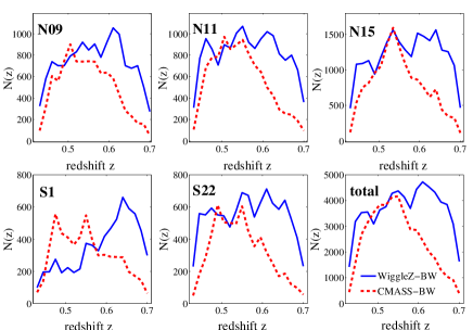
Figure 2: Number of galaxies as a function of redshift for WiggleZ (blue) and CMASS (red) galaxies in the overlap regions, and for the overall overlap volume (bottom right panel).

2.4 Simulations and mock catalogs

We estimate the covariance of our measurements and test the regime of validity of our RSD models using mock galaxy catalogs built from N-body simulations. The conventional methods to generate N-body simulations do not allow for the generation of a large number of realisations of cosmological volumes at sufficient mass resolution to encompass the low-mass halos hosting WiggleZ galaxies, which are needed for constructing robust covariance matrices. For this reason we use an approximate, fast method to generate dark matter simulations based on the COmoving Lagrangian Acceleration method (COLA, Tassev, Zaldarriaga, & Eisenstein, 2013). We have developed a parallel version of COLA (Koda et al., in preparation, used first in Kazin et al., 2014), where in each simulation contains $1296^{3}$ particles in a box of side $600h^{-1}\mathrm{Mpc}$, which gives a particle mass of $7.5\times 10^{9}h^{-1}M_{\odot}$, allowing resolution of low-biased halos with masses $10^{12}$ $h^{-1}M_{\odot}$, found using friends-of-friends algorithm with a linking length of $0.2$ times the mean particle separation. Each simulation requires 15 minutes with 216 computation cores, including halo finding, which is much faster than a classical N-body simulation, but with similar precision on the relevant scales ($k<1$ $h$Mpc^-1).

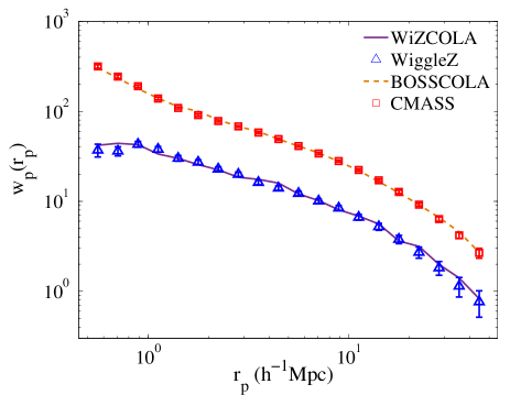
Figure 3: Projected correlation function $w_{p}(r_{p})$ for WiggleZ and CMASS galaxies in the overlap regions (symbols). Lines are the mean values of $w_{p}(r_{p})$ for the COLA mock catalogs.

We generate a total of 2400 realisations (480 for each WiggleZ region) of a flat $\Lambda$CDM universe with WMAP5 cosmological parameters (Komatsu et al., 2009), which defines our fiducial cosmology. Using the output at $z=0.6$ we create WiggleZ-based (WiZcola) and CMASS-based (BOSScola) mock galaxy catalogs, from simple Halo Occupation Distribution models (Berlind & Weinberg, 2002; Blake et al., 2008), such that the resulting projected correlation functions $w_{\rm p}(r_{\rm p})$ match those of the observations, as seen in Figure 3. We then apply the relevant selection functions to the mock galaxies to match the survey geometry. Our simulations encode the joint covariance in the overlapping survey regions (Koda et al., in prep.).

3 Measurements

3.1 Measuring Correlation Functions

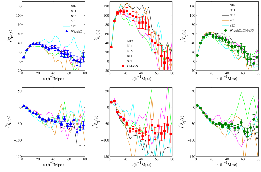
Figure 4: Combined monopole (top row) and quadrupole (bottom row) of $\xi(s,\mu)$ for the WiggleZ and CMASS auto-correlation function (left and middle columns) and the cross-correlation function (right column). Lines are measurements of individual regions, symbols display the combined measurements. Results are plotted as $s^{2}\xi_{l}(s)$ as a function of separation $s$.

We estimate the redshift-space two-point correlation function $\xi(s,\mu)$ (2PCF) as a function of comoving separation $s$ and the cosine of the angle of the distance vector with respect to the line of sight $\mu=\cos(\theta)$. We use the Landy & Szalay (1993) estimator, counting pairs of objects in data and random catalogs:

$$\xi_{\rm auto}(s,\mu)=\frac{DD(s,\mu)-2DR(s,\mu)+RR(s,\mu)}{RR(s,\mu)},$$ (1)

where $DD$, $DR$ and $RR$ are respectively the weight-normalised data-data, data-random and random-random pairs with separation $s$ and $\mu$ (with a given resolution $\Delta s$, $\Delta\mu$). For both the random and data catalogs we use the optimal (inverse-density) FKP weighting (Feldman et al., 1994):

$$w_{i}({\bf x})=\frac{1}{1+n({\bf x})P_{0}}$$ (2)

where $P_{0}=5000$ $(h^{-1}$Mpc)³ for WiggleZ-BW and $P_{0}=20000$ $(h^{-1}$Mpc)³ for CMASS-BW galaxies. For WiggleZ galaxies, angular incompleteness and radial selection are introduced in the random catalogs (Blake et al., 2010). A small fraction of galaxies contain errors in the redshift assignment, but this effect is absorbed into the fitted galaxy bias factor. CMASS galaxies, have additional weights applied to account for the angular incompleteness, fibre collisions, redshift failure and correlation between density of targets and density of stars (Ross et al., 2012).

It is possible to model the 2PCF using the full information from $\xi(s,\mu)$, but that requires a large covariance matrix with the associated problems with its inversion. For this reason it is standard to compress this information in multipoles

$$\xi_{l}(s)=\frac{2l+1}{2}\int_{-1}^{1}\xi(s,\mu)L_{l}(\mu)d\mu,$$ (3)

where $L_{l}$ is the Legendre polynomial of order $l$. In practice we approximate eq. (3) by a discrete sum over the binned $\xi(s,\mu)$, where we use $\Delta s=4$ $h^{-1}$Mpc and $\Delta\mu$=0.01 for every WiggleZ-BW and CMASS-BW region. We use the monopole ($l=0$) and quadrupole ($l=2$) of the 2-point functions, to analyse the redshift-space distortions, for separations $s<80$ $h^{-1}$Mpc. Our results are unchanged if large separations are used, whilst the increase in variance due to the finite number of mocks becomes significant.

The covariance of each region is estimated from the mock WiZcola and BOSScola catalogs (see section 3.3). After calculating the covariances of the measurements in each overlap region from the COLA mock catalogs, we use inverse-variance weighting to obtain the ‘optimally combined’ measurements. For the statistic $\xi_{l,\rm{comb}}(s)$, the optimally combined function is calculated as

$$\xi_{l,\rm{comb}}(s)=\mathcal{C}_{\rm{comb}}\sum_{i=1}^{N_{reg}}\mathcal{C}_{i}^{-1}\xi_{l,i}(s)$$ (4)

where $\mathcal{C}_{\rm{comb}}$ is the overall covariance matrix, calculated from the estimations of the covariance matrices of individual regions $\mathcal{C}_{i}$ (see section 3.3). Results for the auto-2PCFs are shown in Figure 4, for individual regions (as lines) and for the combined measurements (as symbols). The different amplitude of clustering of the WiggleZ-BW and CMASS-BW galaxies reflects the difference in the type of halos these galaxies inhabit. Due to the limited volume where the correlations are measured, we correct our correlation function values by the ‘integral constraint’ (Peebles, 1980; Beutler et al., 2012). The corrections to the WiggleZ and BOSS correlations differ in each region and have values of the order of $8\times 10^{-4}$ and $1\times 10^{-3}$ respectively for the smaller regions (where the integral constraint is higher), and do not significantly affect the RSD model constraints.

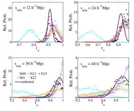
Figure 5: The cross-correlation coefficient $r_{\times}$ for the WiggleZ-CMASS-BW correlations for each overlap regions, and when combining all regions, as a function of the smallest scale $s_{min}$ (in $h^{-1}$Mpc) of the fit.

3.2 Cross-correlations between WiggleZ-BW and CMASS-BW clustering

In addition to the auto-correlations, we also measured the cross-correlation between the two sets for tracers using the estimator

$$\xi_{\rm cross}(s,\mu)=\frac{D_{W}D_{C}-D_{W}R_{C}-R_{W}D_{C}+R_{W}R_{C}}{R_{W}R_{C}},$$ (5)

where the $W$ and $C$ subscripts represent the quantities in the WiggleZ and CMASS galaxies, respectively. The cross-correlation function measurement provides an independent validation of the assumption that both galaxy types trace the same large structures on a range of scales, and also serves to test our linear and local galaxy bias model.

To test the strength of the correlation between the tracers is, we also constrain the cross-correlation coefficient, $r_{\times}$, which is produced from the relation

$$\xi^{l=0}_{\rm WiggleZ\times CMASS}(s)=r^{2}_{\times}(s)\xi^{l=0}_{\rm WiggleZ}(s)\xi^{l=0}_{\rm CMASS}(s),$$ (6)

with $|r_{\times}|\leq 1$. On large scales in redshift-space, and assuming linear, deterministic bias, this quantity should tend to the value (Mountrichas et al., 2009):

$$r_{\times,{\rm Kaiser}}=\frac{1+\frac{1}{3}(\beta_{W}+\beta_{C})+\frac{1}{5}\beta_{W}\beta_{C}}{\sqrt{\left(1+\frac{2}{3}\beta_{W}+\frac{1}{5}\beta_{W}^{2}\right)\left(1+\frac{2}{3}\beta_{C}+\frac{1}{5}\beta_{C}^{2}\right)}}$$ (7)

Assuming $b_{W}=1$ and $b_{C}=2$ (Reid et al., 2012; Contreras et al., 2013), and a growth rate $f(z=0.54)=0.75$, when estimating $\beta=f/b$, it is expected that $r_{\times,{\rm Kaiser}}=0.997\sim 1$.

We measure the value of $r_{\times}$ from our data, assuming it is a constant on all scales (an assumption we do not expect to hold on scales smaller than $~{}15-20$ $h^{-1}$Mpc). Using the redshift space distortion model described in section 4.1, and the COLA mocks to build our covariance matrix, we use the correlation monopoles to fit for the bias parameters of the WiggleZ-BW and CMASS-BW galaxies and $r_{\times}$ for each overlap region and the joint likelihood (see section 4.3 for details of the fitting procedure).

Figure 5 presents the posterior probability distribution of $r_{\times}$, as a function of the minimum scale of fit $s_{min}$. Focusing on the fits to the combined regions, we can see that they are not consistent with $r_{\times}=1$ at the $2\sigma$ level on scales $s_{min}\sim 20$ $h^{-1}$Mpc. This behaviour may be explained by a number of factors such as non-linear pairwise velocities, non-linear bias and stochasticity. CMASS galaxies tend to be hosted in the centres of large halos and in high density regions, precisely the regions that are avoided by WiggleZ galaxies. We expect that on large scales both galaxies trace similar structures, and this is confirmed in the measurements of $r_{\times}$ being consistent with 1 when fitting on large scales.

Examining individual regions it can be noticed that it is region S22 which reduces the overall fit to $r_{\times}$. Its lower value of $r_{\times}$ is driven by a high auto-correlation function in the WiggleZ-BW S22 region, although the scatter is compatible with the variance against mock catalogs. The best fits to the growth rate do not significantly change when the S22 region is excluded, and in the final fits we include all regions.

3.3 Covariance estimation

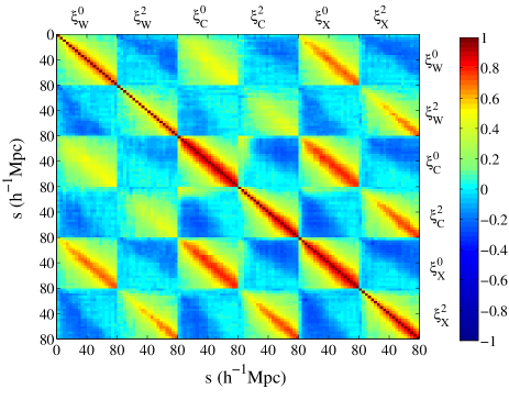
Figure 6: Correlation matrix (normalised covariance matrix) of the WiggleZ-CMASS multipoles based on COLA mocks. The matrix is divided in the contributions from the monopole and quadrupole of WiggleZ-BW (W), CMASS-BW (C) and cross 2PCFS (X), and each pixel represents a separation s (in $h^{-1}$Mpc).

We estimate the correlations between the multipoles of the auto- and cross-2PCF by calculating the covariance matrix in each region $n$ from COLA mocks. A deviation from the mean of a quantity $X$, in separation bin $i$, for the mock $k$ can be written as

$$\Delta_{i,n}^{k}=X_{i}^{k}-\langle X_{i}\rangle$$ (8)

where, in our case, $X$ corresponds to the monopole or quadrupole of the auto- or cross-2PCF in each bin. The covariance matrix of each region $n$ is determined as

$$\mathcal{C}_{n,ij}=\frac{1}{N_{\rm mocks}}\sum_{k=1}^{N_{\rm mocks}}\Delta_{i,n}^{k}\Delta_{j,n}^{k}$$ (9)

After calculating $\mathcal{C}_{n}$ for all regions, we can determine the combined covariance matrix (Blake et al., 2011a)

$$\mathcal{C}^{-1}_{comb}=\sum_{n=1}^{N_{reg}}\mathcal{C}_{n}^{-1}$$ (10)

Figure 6 shows the correlation matrix (normalised covariance matrix) for all our measurements, showing the strong correlation between the measurements of the two tracers.

Since we used a large, but finite number of mock catalogs for the covariance estimation, there is an underestimation of the uncertainties. Following the work of Hartlap et al. (2007); Percival et al. (2014), we correct for the finite number of mocks by multiplying the variance estimated from the likelihood distribution by

$$m_{\sigma}=\frac{1+B(N_{\rm bins}-N_{\rm p})}{1+2A+N(N_{\rm p}+1)}$$ (11)

where $N_{\rm bins}$ is the number of bins entering the fits, $N_{\rm p}$ is the number of free parameters, and

$$A^{-1} = (N_{\rm mocks}-N_{\rm bins}-1)(N_{\rm mocks}-N_{\rm bins}-4),$$ (12)

$$B = A(N_{\rm mocks}-N_{\rm bins}-2),$$ (13)

where $N_{\rm mocks}$ is the number of mock realisations. Also, the sample variance should be multiplied by

$$m_{v}=m_{\sigma}\frac{N_{\rm mocks}-1}{N_{\rm mocks}-N_{\rm bins}-2}.$$ (14)

We use $N_{\rm mocks}=480$ and perform measurements in separation bins up to $s=80$ $h^{-1}$Mpc. From constraining models using one-tracer auto-correlation function multipoles to simultaneous fits using both auto and cross correlations, the $m_{v}$ factor lies in the range $m_{v}=1.1-1.45$.

4 Constraints on cosmic growth

4.1 Modelling the RSD

Redshift-space distortions modify the 2-point clustering of galaxies on both large and small scales, which we will summarise here. Due to its peculiar velocity ${\bf v}$, a galaxy at a position in real space ${\bf r}$ gets mapped to ${\bf s}$ in redshift space:

$${\bf s}={\bf r}+\frac{(1+z){\bf v}\cdot\hat{r}}{H(z)}\hat{r}$$ (15)

where $\hat{r}$ is the galaxy unit vector along the line of sight (LOS) direction, $v_{r}\equiv{\bf v}\cdot\hat{r}$ is the line-of-sight component of its velocity, and $H(z)$ is the Hubble parameter at a redshift $z$.

On large scales, as described by Kaiser (1987), hereafter K87 (also see Hamilton 1998 for derivations in configuration space), matter overdensities $\delta_{m}$ grow coherently as $\nabla\cdot{\bf v}\propto-f\delta_{m}$ where $f\equiv d\ln G(a)/d\ln a$ is the linear growth rate of fluctuations. The evolution of the growth rate in certain models can be approximated by the evolution of the matter density in the universe $f(z)=\Omega_{m}(z)^{\gamma}$, where $\gamma=0.55$ in the case that the large-scale gravity obeys General Relativity; for alternative theories of gravity, $\gamma$ can take on different values (Linder & Cahn, 2007). If we assume that the difference in clustering between dark matter and galaxies can be described by a linear bias model where $\delta_{g}=b\,\delta_{m}$ then in Fourier space the redshift space galaxy overdensity takes the form

$$\delta_{g}({\bf k})=(b+f\mu^{2})\delta_{m}({\bf k}),$$ (16)

creating in configuration space the so-called ‘squashing’ effect on large scales.

On small scales, in the non-linear regime for overdensities and velocities, large structures appear elongated along the line of sight, creating the observed ‘Fingers of God’. In Fourier space this effect can be modelled by multiplying a Gaussian or a Lorentzian pairwise velocity distribution (i.e. a convolution of a Gaussian or exponential profile in configuration space) into the large-scale redshift-space distortion of the power spectrum. The simplest model, using Gaussian damping for the galaxy power spectrum in redshift space, is

$$P^{s}(k,\mu)=(b+f\mu^{2})^{2}P_{m}(k)e^{-(k\mu\sigma_{v}/H)^{2}}$$ (17)

$P_{m}(k)$ represents the non-linear real-space power spectrum and $\sigma_{v}$ the pairwise velocity dispersion, which we approximate to be the same for all tracers is predicted to be

$$\sigma_{v}^{2}(z)=\frac{f^{2}(z)H^{2}(z)}{6\pi^{2}(1+z)^{2}}\int P_{\theta\theta}(k)dk$$ (18)

where, in the K87 formalism, $P_{\theta\theta}=P_{m}$. However, this simple model has been shown in simulations to be insufficiently accurate even on large scales, because there is not a perfect correlation between density and the velocity (divergence) field (e.g Okumura & Jing, 2011; Kwan et al., 2012; de la Torre & Guzzo, 2012; White et al., 2014). Scoccimarro (2004), hereafter S04, suggested a modification of the simple Kaiser formalism by including the velocity field terms. In the case of one tracer, the RSD in the galaxy auto- power spectrum reads:

$$P^{s}_{\rm a}(k,\mu)=[b^{2}P_{\delta\delta}(k)+2\mu^{2}fbP_{\delta\theta}(k)+\mu^{4}f^{2}P_{\theta\theta}(k)]e^{-(k\mu\sigma_{v}/H)^{2}}$$ (19)

where $P_{\delta\delta}$, $P_{\delta\theta}$ and $P_{\theta\theta}$ are the non-linear matter density-density, density-velocity and velocity-velocity power spectra, respectively. In our analysis, these terms are obtained from fitting formulae derived by Jennings (2012), from a suite of N-body simulations. In this case our fiducial model (based on WMAP5 results, see $\S$1) predicts (via Eq.18) the large-scale velocity dispersion $\sigma_{v}$ to be $\sigma_{v}(z=0.6)\sim 220$ kms^-1. However, we choose to leave $\sigma_{v}$ as a free parameter to account for any additional non-linearities on smaller scales. Whilst there are additional improvements and implementations of RSD models (e.g. Taruya et al., 2010; Seljak & McDonald, 2011; Reid & White, 2011; Wang et al., 2013), this particular formalism has been successfully used in a number of studies (e.g. Blake et al., 2011b; de la Torre et al., 2013; Blake et al., 2013), and, as we will see below, reproduces the expected constraints on the growth rate from the COLA mock catalogs and provides a good description of the galaxy anisotropic clustering at the current statistical level.

In the case of the redshift-space cross-power spectrum, assuming that both tracers are described by the same dispersion parameter $\sigma_{v}$, we can write the large-scale terms as

$$P^{s}_{\rm x}(k,\mu) = [b_{1}b_{2}P_{\delta\delta}(k)+\mu^{2}f(b_{1}+b_{2})P_{\delta\theta}(k)+$$ (20)

$$\mu^{4}f^{2}P_{\theta\theta}(k)]\times e^{-(k\mu\sigma_{v}/H(z))^{2}}$$

where $b_{1}$ and $b_{2}$ are the biases of the different tracers. Since we are measuring the multipoles of the 2PCF, we calculate first the power spectrum multipoles as

$$P^{s}_{l}(k)=\frac{2l+1}{2}\int_{-1}^{1}P^{s}(k,\mu)L_{l}(\mu)d\mu,$$ (21)

where $l$ is the multipole order and $L_{l}$ is the Legendre polynomial of order $l$. Then for the 2-point correlation function in configuration space we have

$$\xi^{s}_{l}(s)=\frac{i^{l}}{2\pi^{2}}\int P^{s}_{l}(k)j_{l}(ks)k^{2}dk$$ (22)

where $j_{l}$ is the spherical Bessel function of order $l$.

4.2 Tests using COLA mocks

We tested the validity of these models using our COLA mock catalogs. In summary, we compared the K87 and S04 models for the large-scale distortions to $P(k)$ (calculated using our fiducial cosmological parameters), using a Gaussian function for the small-scale damping (we also tried fits using the Lorentzian profile without significant differences), constraining the growth rate $f$ at the simulation output redshift $z=0.6$, marginalising over the bias of each tracer and the common velocity dispersion $\sigma_{v}$. We performed these fits for every COLA mock on scales $s<80$ $h^{-1}$Mpc, although changes when using larger scales were not significant.

Figure 7 shows the mean and standard deviation of the best-fitting values of $f(z=0.6)$ across the mocks. For the WiZcola mocks the K87+Gaussian model tends to underpredict the value of the growth rate whereas the S04+Gaussian model agrees well for scales $s_{\rm min}>20$ $h^{-1}$Mpc. For the BOSScola mocks the differences are less pronounced, but the input growth rate is recovered with a systematic error less than the statistical error. In both cases the goodness of fit is similar with $\chi^{2}$/d.o.f.$\sim 1$ for both WiggleZ and BOSS COLA mocks on larger scales $s_{\rm min}>20$ $h^{-1}$Mpc, worsening considerably on scales $s_{\rm min}<10$ $h^{-1}$Mpc. In what follows we will use the S04+Gaussian model for our parameter fits.

There are, however, specific differences in the scale of validity of the models depending on which tracer is used. It can be seen that for low-bias galaxies represented by the WiZcola mocks, the agreement between the model fits and the input value of $f(z=0.6)$ extends to lower scales than in the case of galaxies residing in more massive halos. Although the Kaiser effect is stronger for lower bias galaxies, the higher non-linearities arising from the formation and high-clustering of high-mass halos lead to a model break-down on larger scales. For the particular case of the WiggleZ-BOSS overlap, $s_{min}=24$ $h^{-1}$Mpc is the minimum scale where both models recover adequately the fiducial growth rate with negligible systematic error.

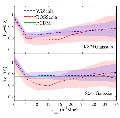
Figure 7: Constraints on the linear growth rate $f(z=0.6)$ using COLA mock galaxies with the same angular and redshift selection functions as the galaxy survey data. Fits to the growth rate $f(z=0.6)$ ($=0.76$, for the WMAP5 cosmology, green solid line) are performed for the models as a function of $s_{min}$, with $s_{max}=80$ $h^{-1}$Mpc. Colored shades cover the 1$\sigma$ (68%) confidence interval for $f$, defined using the dispersion in the best-fitting values across the 480 mocks.

Multitracer approach

Having chosen the model to analyse redshift-space clustering, we examined the consequences of using multiple tracers when recovering model parameters. For each realisation of the COLA mocks we fit the S04+Gaussian RSD model first using the autocorrelations independently, then analysing both autocorrelations but considering the common covariance matrix, and lastly adding the cross-correlations using the monopole and quadrupole of $\xi(s,\mu)$ in the range $24<s<80$ $h^{-1}$Mpc. Results are shown in Figure 8, which displays the 1$\sigma$ contours enclosing the best-fitting values of $f(z=0.6)$ and $\sigma_{v}$. The expected values for these parameters are consistent with our COLA constraints, and the approximation that $\sigma_{v}$ is the same for both tracers is valid for this range of scales. The constraints for the parameters are correlated between the two surveys, with a cross-correlation coefficient $\rho^{f}_{WC}=\sigma^{f}_{WC}/\sigma^{f}_{W}\sigma^{f}_{C}=0.4$ for the growth rate between both surveys.

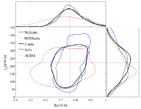
Figure 8: Constraints for RSD parameters in the S04 model for fits to COLA mocks in the range $24<s<80$ $h^{-1}$Mpc using 2PCF multipoles. Results for the full fit and for individual subsamples, with the contours enclosing 68% of the best-fitting parameters are shown. The four cases considered are WiZcola mocks alone (blue solid line), BOSScola mocks alone (red dashed line), joint analysis of the auto-correlations (black solid line), and an analysis further adding the cross-correlation function (green dashed line).

When analysing the 2PCFs of the two tracers simultaneously, taking into account the common covariance, an improvement in the measurement of $f$ is obtained, of the order 30% compared to using the BOSScola mocks alone (which because of a higher bias, have a lower value of $\beta$ and hence a lower signal) but only 5% compared to using WiZcola mocks alone. Adding the cross-2PCF produces an improvement of 20% compared to the WiZcola-only constraints, mostly due to an increased signal in the shot-noise dominated regime. Analysing individual mocks shows that the improvement also varies in each realisation. As predicted by McDonald & Seljak (2009), Gil-Marín et al. (2010) and Blake et al. (2013), although our tracers have big differences in their biasing, due to the sparsity of our sampling we are in the regime where shot noise dominates and improvement via the cancellation of cosmic variance is small.

4.3 Data Fitting procedure

In our analysis we fixed the cosmological parameters of the matter power spectra to the best-fit WMAP5 model (Komatsu et al., 2009), the fiducial cosmology of our COLA mocks, and constrain the parameters $(b_{W},b_{C},f(z=0.54),\sigma_{v})$. Due to the degeneracy of the first three parameters with $\sigma_{8}(z)$, the r.m.s. of the matter density field in 8 $h^{-1}$Mpc spheres, we are effectively constraining $(b_{W}\sigma_{8},b_{C}\sigma_{8},f\sigma_{8},\sigma_{v})$. When we also include the WiggleZ-CMASS cross-correlation in the analysis, we additionally fit for the parameter $r_{\times}$. We compare the constraints from the single-tracer model for each galaxy type to each other, and then include the common covariance and the cross-correlations in the cosmological fits.

We use the monopole and quadrupole of the tracers, and present results as a function of the minimum-scale fitted $s_{\rm min}$, with $s_{max}=80$ $h^{-1}$Mpc. We execute a Maximum Likelihood parameter estimation test, where we minimise the quantity

$$\chi^{2}=\sum_{i}\sum_{j}(X_{i,{\rm model}}-X_{i,{\rm data}})\mathcal{C}_{comb,ij}^{-1}(X_{j,{\rm model}}-X_{j,{\rm data}}),$$ (23)

where $X$ is one of the elements of the vector formed by the multipoles of $\xi(s,\mu)$ of WiggleZ-BW, CMASS-BW and/or WiggleZ-CMASS-BW correlations. We explore the parameter space using a Monte Carlo Markov Chain method (MCMC) imposing the prior that all parameter values must be bigger than zero.

4.4 Fits for the growth rate

Figure 9 presents the parameter fits of $f\sigma_{8}(z=0.54)$ fitting the monopole and quadrupole of the WiggleZ and CMASS auto- and cross-correlation on scales between $s_{min}=24$ $h^{-1}$Mpc, and $s_{max}=80$ $h^{-1}$Mpc. As shown in the previous section, $s_{\rm min}=24$ $h^{-1}$Mpc is the minimum scale where there are not important systematic deviations in the parameters from the study with the COLA mocks, and our fits to the observed data follow this trend. Table 2 lists the results for the parameter fits.

Comparing the single-tracer fits for WiggleZ-BW and CMASS-BW galaxies, there is agreement at the $1\sigma$ level for the values of $f\sigma_{8}(z=0.54)$, meaning that when fitting to these scales there is evidence of no systematics depending on the type of galaxy used. Our constraints on the growth rate are consistent with our fiducial cosmology $f\sigma_{8}(z=0.54)=0.46$.

Consistent with previous work, we recover that the bias of the WiggleZ-BW galaxies, $b_{W}\sim 1$, is smaller than that of the CMASS-BW galaxies, $b_{C}\sim 2$. The value of the best-fitting chi-squared statistic indicates that the model provides a reasonable fit to the data in all cases. For the pairwise dispersion, values for the different tracers are consistent with the predicted value from theory (section 4.1).

Combining the two tracers including their cross-covariance yields slightly better constraints for $f\sigma_{8}(z=0.54)$ at the level of 10% (compared to WiggleZ constraints alone). This result indicates that for these tracers, in a low density regime (where the common cosmic variance cancellation does not improve the constraints, see Blake et. al 2013), even in the presence of a slightly larger Hartlap-Percival correction, the improvement is due to reduced shot noise. When including the cross-correlations the improvement is of the order of 20% (again, compared with WiggleZ constraints alone). In the case when we include the cross-correlations, we obtain our poorest value for $\chi^{2}/$d.o.f., implying that our simple constant $r_{\times}$ model may not describe all of the complexities of the cross-correlation. Given this result, we quote as result of our paper for the growth rate constraint the one obtained when we combine only the auto-correlations, yielding $f\sigma_{8}(z=0.54)=0.413\pm 0.054$.

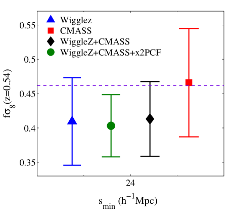
Figure 9: Fits to the RSD model parameters using correlation multipoles with $24<s<80$ $h^{-1}$Mpc. We show results when analysing individual surveys and joint constraints. The purple line shows the prediction from WMAP5 cosmology.

Table 2: Fits to the RSD model parameters when using multipoles with $24<s<80$ $h^{-1}$Mpc assuming WMAP5 $\sigma_{8}(z=0)=0.812$

Tracers	$b_{W}\sigma_{8}(z=0.54)$	$b_{C}\sigma_{8}(z=0.54)$	$f\sigma_{8}(z=0.54)$	$\sigma_{v}$ (kms-1)	$r_{\times}$	$\chi^{2}$/d.o.f	d.o.f.
WiggleZ only	0.651$\pm$0.046	-	0.409$\pm$0.059	205$\pm$144	-	1.11	28 - 4
CMASS only	-	1.204$\pm$0.062	0.466$\pm$0.074	130$\pm$116	-	1.43	28 - 4
WiggleZ+CMASS	0.646$\pm$0.043	1.233 $\pm$0.054	0.413$\pm$0.054	117$\pm$113	-	1.28	56 - 5
WiggleZ+CMASS+x2PCF	0.648$\pm$0.038	1.242$\pm$0.043	0.403$\pm$0.048	88$\pm$104	0.93 $\pm$ 0.03	1.57	84 - 6

5 Summary & Conclusions

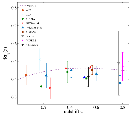
Figure 10: Fits to the growth rate $f\sigma_{8}(z)$ from different galaxy surveys: 6dF (Beutler et al., 2012), 2dFGRS (Hawkins et al., 2003), GAMA (Blake et al., 2013), WiggleZ (Blake et al., 2011b), SDSS LRGs (Samushia et al., 2012), CMASS-DR9 (Reid et al., 2012), VVDS(Guzzo et al., 2008), and VIPERS (de la Torre et al., 2013).

In this work we have presented the first cosmological RSD analysis using data from two overlapping surveys, WiggleZ and CMASS. After defining the overlap volumes, we measured 2-point auto- and cross-correlations functions of these tracers; after obtaining their multipoles and calculating their cross-covariance using N-body mock catalogs, we compared them with RSD models in order to measure the growth rate of structure $f\sigma_{8}$ at an effective redshift $z=0.54$. Our main findings are:

• The cross-correlation coefficient $r_{\times}$ between the WiggleZ-BW and CMASS-BW galaxies agrees with the expectation that on large scales, the two classes trace similarly the large scale structure with $r_{\times}\sim 1$. On smaller scales $s\lesssim 20$ $h^{-1}$Mpc, $r_{\times}<1$, likely produced by a combination of a number of factors such as non-linear pairwise velocities, non-linear bias and stochasticity.

• We tested redshift-space distortion models in mock catalogues simulating WiggleZ and CMASS galaxies, including the selection functions of our overlapping volumes. When fitting scales $s>24$ $h^{-1}$Mpc we recover our fiducial cosmological parameters using different tracers, and that a single velocity dispersion provides an adequate description for the distortions in our range of scales. We confirmed a lack of a significant improvement when using the multitracer technique, given the sparsity of the sampling for these tracers.

• The fits to $f\sigma_{8}(z)$ from all tracers are consistent with each other and with the predictions of a $\Lambda$CDM universe, showing no evidence for strong modelling systematic errors as a function of galaxy type.

As shown in Figure 10, our combined fit for the growth rate $f\sigma_{8}(z=0.54)=0.413\pm 0.054$ is in excellent agreement with estimates from different surveys. Although more sophisticated models for the RSD can be employed, the motivation for our work was to show consistency in the cosmological fits when using different tracers. This agreement provides further strong evidence for the robustness in the growth rate measurements which are important for answering the outstanding questions on the nature of dark energy and large-scale gravity.

We thank Ariel Sánchez, Héctor Gil-Marín, Tamara Davis, David Parkinson, Raúl Angulo, Andrew Johnson, Luis Torres, Shahab Joudaki and Caitlin Adams, for enlightening discussions and comments to this work. FM, CB, EK, JK were supported by the Australian Research Council Centre of Excellence for All-Sky Astrophysics (CAASTRO) through project number CE110001020. CB acknowledges the support of the Australian Research Council through the award of a Future Fellowship. This work was performed on the gSTAR national facility at Swinburne University of Technology. gSTAR is funded by Swinburne and the Australian Governments Education Investment Fund. This research has made use of NASA’s Astrophysics Data System.

Funding for SDSS-III has been provided by the Alfred P. Sloan Foundation, the Participating Institutions, the National Science Foundation, and the U.S. Department of Energy. SDSS-III is managed by the Astrophysical Research Consortium for the Participating Institutions of the SDSSIII Collaboration including the University of Arizona, the Brazilian Participation Group, Brookhaven National Laboratory, University of Cambridge, Carnegie Mellon University, University of Florida, the French Participation Group, the German Participation Group, Harvard University, the Instituto de Astrofísica de Canarias, the Michigan State/Notre Dame/JINA Participation Group, Johns Hopkins University, Lawrence Berkeley National Laboratory, Max Planck Institute for Astrophysics, Max Planck Institute for Extraterrestrial Physics, New Mexico State University, New York University, Ohio State University, Pennsylvania State University, University of Portsmouth, Princeton University, the Spanish Participation Group, University of Tokyo, University of Utah, Vanderbilt University, University of Virginia, University of Washington, and Yale University.

References

- Adelman-McCarthy et al. (2006) Adelman-McCarthy J. K., et al., 2006, ApJS, 162, 38
- Alam et al. (2015) Alam S. et al., 2015, ArXiv e-prints
- Asorey et al. (2013) Asorey J., Crocce M., Gaztanaga E., 2013, ArXiv e-prints
- Berlind & Weinberg (2002) Berlind A. A., Weinberg D. H., 2002, ApJ, 575, 587
- Bernstein & Cai (2011) Bernstein G. M., Cai Y.-C., 2011, MNRAS, 416, 3009
- Beutler et al. (2012) Beutler F. et al., 2012, Monthly Notices of the Royal Astronomical Society, 423, 3430
- Beutler et al. (2014) Beutler F. et al., 2014, MNRAS, 443, 1065
- Blake et al. (2013) Blake C. et al., 2013, MNRAS, 436, 3089
- Blake et al. (2008) Blake C., Collister A., Lahav O., 2008, MNRAS, 385, 1257
- Blake et al. (2011a) Blake C. et al., 2011a, MNRAS, 418, 1725
- Blake et al. (2010) Blake C., et al., 2010, MNRAS, 406, 803
- Blake et al. (2011b) Blake C., et al., 2011b, MNRAS, 415, 2876
- Bolton et al. (2012) Bolton A. S. et al., 2012, AJ, 144, 144
- Chen (2009) Chen J., 2009, A&A, 494, 867
- Chuang et al. (2013) Chuang C.-H. et al., 2013, MNRAS, 433, 3559
- Contreras et al. (2013) Contreras C. et al., 2013, arXiv.org
- Croft (2013) Croft R. A. C., 2013, arXiv.org
- Dawson et al. (2013) Dawson K. S. et al., 2013, AJ, 145, 10
- de la Torre & Guzzo (2012) de la Torre S., Guzzo L., 2012, Monthly Notices of the Royal Astronomical Society, 427, 327
- de la Torre et al. (2013) de la Torre S. et al., 2013, arXiv.org
- Drinkwater et al. (2010) Drinkwater M. J., et al., 2010, MNRAS, 401, 1429
- Eisenstein et al. (2011) Eisenstein D. J. et al., 2011, The Astronomical Journal, 142, 72
- Feldman et al. (1994) Feldman H. A., Kaiser N., Peacock J. A., 1994, ApJ, 426, 23
- Font-Ribera et al. (2013) Font-Ribera A. et al., 2013, JCAP, 5, 18
- Gaztañaga et al. (2012) Gaztañaga E., Eriksen M., Crocce M., Castander F. J., Fosalba P., Marti P., Miquel R., Cabré A., 2012, MNRAS, 422, 2904
- Gil-Marín et al. (2010) Gil-Marín H., Wagner C., Verde L., Jimenez R., Heavens A. F., 2010, Monthly Notices of the Royal Astronomical Society, 407, 772
- Gilbank et al. (2011) Gilbank D. G., Gladders M. D., Yee H. K. C., Hsieh B. C., 2011, AJ, 141, 94
- Gunn et al. (2006) Gunn J. E. et al., 2006, AJ, 131, 2332
- Guzzo et al. (2008) Guzzo L. et al., 2008, Nature, 451, 541
- Hamilton (1998) Hamilton A. J. S., 1998, in Astrophysics and Space Science Library, Vol. 231, The Evolving Universe, Hamilton D., ed., p. 185
- Hartlap et al. (2007) Hartlap J., Simon P., Schneider P., 2007, A&A, 464, 399
- Hawkins et al. (2003) Hawkins E., et al., 2003, MNRAS, 346, 78
- Jennings (2012) Jennings E., 2012, MNRAS, 427, L25
- Kaiser (1986) Kaiser N., 1986, MNRAS, 219, 785
- Kaiser (1987) Kaiser N., 1987, Monthly Notices of the Royal Astronomical Society (ISSN 0035-8711), 227, 1
- Kazin et al. (2014) Kazin E. A. et al., 2014, MNRAS, 441, 3524
- Kazin et al. (2013) Kazin E. A. et al., 2013, ArXiv e-prints
- Komatsu et al. (2009) Komatsu E., et al., 2009, ApJS, 180, 330
- Kwan et al. (2012) Kwan J., Lewis G. F., Linder E. V., 2012, ApJ, 748, 78
- Landy & Szalay (1993) Landy S. D., Szalay A. S., 1993, ApJ, 412, 64
- Linder & Cahn (2007) Linder E. V., Cahn R. N., 2007, Astroparticle Physics, 28, 481
- Lombriser et al. (2013) Lombriser L., Yoo J., Koyama K., 2013, Phys. Rev. D, 87, 104019
- Marín et al. (2013) Marín F. A. et al., 2013, MNRAS, 432, 2654
- Martin et al. (2005) Martin D. C., et al., 2005, ApJ, 619, L1
- Martínez et al. (1999) Martínez H. J., Merchán M. E., Valotto C. A., Lambas D. G., 1999, ApJ, 514, 558
- McDonald & Seljak (2009) McDonald P., Seljak U., 2009, Journal of Cosmology and Astroparticle Physics, 2009, 007
- Mountrichas et al. (2009) Mountrichas G., Sawangwit U., Shanks T., Croom S. M., Schneider D. P., Myers A. D., Pimbblet K., 2009, Monthly Notices of the Royal Astronomical Society, 394, 2050
- Okumura & Jing (2011) Okumura T., Jing Y. P., 2011, ApJ, 726, 5
- Peacock (1992) Peacock J. A., 1992, in Lecture Notes in Physics, Berlin Springer Verlag, Vol. 408, New Insights into the Universe, Martinez V. J., Portilla M., Saez D., eds., p. 1
- Peacock et al. (2001) Peacock J. A., et al., 2001, Nature, 410, 169
- Peebles (1980) Peebles P. J. E., 1980, The large-scale structure of the universe
- Percival et al. (2014) Percival W. J. et al., 2014, MNRAS, 439, 2531
- Reid et al. (2012) Reid B. A. et al., 2012, Monthly Notices of the Royal Astronomical Society, 426, 2719
- Reid & White (2011) Reid B. A., White M., 2011, MNRAS, 417, 1913
- Ross et al. (2012) Ross A. J. et al., 2012, MNRAS, 424, 564
- Ross et al. (2014) Ross A. J. et al., 2014, MNRAS, 437, 1109
- Samushia et al. (2012) Samushia L., Percival W. J., Raccanelli A., 2012, MNRAS, 420, 2102
- Sánchez et al. (2013) Sánchez A. G. et al., 2013, arXiv.org
- Scoccimarro (2004) Scoccimarro R., 2004, Physical Review D, 70, 083007
- Seljak (2009) Seljak U., 2009, Physical Review Letters, 102, 021302
- Seljak & McDonald (2011) Seljak U., McDonald P., 2011, Journal of Cosmology and Astroparticle Physics, 11, 039
- Sharp et al. (2006) Sharp R., et al., 2006, in Society of Photo-Optical Instrumentation Engineers (SPIE) Conference Series, Vol. 6269, Society of Photo-Optical Instrumentation Engineers (SPIE) Conference Series
- Smee et al. (2013) Smee S. A. et al., 2013, AJ, 146, 32
- Taruya et al. (2010) Taruya A., Nishimichi T., Saito S., 2010, Physical Review D, 82, 063522
- Tassev et al. (2013) Tassev S., Zaldarriaga M., Eisenstein D. J., 2013, JCAP, 6, 36
- Tojeiro et al. (2012) Tojeiro R. et al., 2012, Monthly Notices of the Royal Astronomical Society, 424, 2339
- Wang et al. (2013) Wang L., Reid B., White M., 2013, arXiv.org
- White et al. (2014) White M., Reid B., Chuang C.-H., Tinker J. L., McBride C. K., Prada F., Samushia L., 2014, ArXiv e-prints
- White et al. (2009) White M., Song Y.-S., Percival W. J., 2009, MNRAS, 397, 1348
- Yoo & Seljak (2013) Yoo J., Seljak U., 2013, ArXiv e-prints