Numerical analysis on local risk-minimization for exponential Lévy models

Abstract

We illustrate how to compute local risk minimization (LRM) of call options for exponential Lévy models. We have previously obtained a representation of LRM for call options; here we transform it into a form that allows use of the fast Fourier transform method suggested by Carr & Madan. In particular, we consider Merton jump-diffusion models and variance gamma models as concrete applications.

Keywords: Local risk minimization; Fast Fourier transform; Exponential Lévy processes; Merton jump-diffusion processes; Variance gamma processes.

1 Introduction

Local risk minimization (LRM), which has more than 20 years’ history, is a well-known hedging method for contingent claims in incomplete markets. Although its theoretical aspects have been very well studied, corresponding computational methods have yet to be thoroughly developed. This paper aims to illustrate how to numerically calculate LRM for call options in exponential Lévy models. To our knowledge, this contribution is the first to address this subject. In Arai & Suzuki [1], we obtained a representation of LRM for call options by using Malliavin calculus for Lévy processes based on the canonical Lévy space. Here we transform that result into a form that allows the fast Fourier transform method suggested by Carr & Madan [4] to be applied. In particular, Merton jump-diffusion and variance gamma models, being common classes of exponential Lévy models, are discussed as concrete applications of our approach.

Consider a financial market composed of one risk-free asset and one risky asset with finite time horizon $T>0$. For simplicity, we assume that the market’s interest rate is zero, that is, the price of the risk-free asset is 1 at all times. The fluctuation of the risky asset is assumed to be described by an exponential Lévy process $S$ on a complete probability space $(\Omega,{\cal F},{\mathbb{P}})$, described by

$$S_{t}:=S_{0}\exp\left\{\mu t+\sigma W_{t}+\int_{{\mathbb{R}}_{0}}x\widetilde{N}([0,t],dx)\right\}\quad\mbox{ for }t\in[0,T]\,,$$

where $S_{0}>0$, $\mu\in{\mathbb{R}}$, $\sigma>0$, and ${\mathbb{R}}_{0}:={\mathbb{R}}\setminus\{0\}$. Here $W$ is a one-dimensional Brownian motion and $\widetilde{N}$ is the compensated version of a Poisson random measure $N$. Denoting the Lévy measure of $N$ by $\nu$, we have $\widetilde{N}([0,t],A)=N([0,t],A)-t\nu(A)$ for any $t\in[0,T]$ and $A\in{\cal B}({\mathbb{R}}_{0})$. Moreover, $S$ is also a solution to the stochastic differential equation

$$dS_{t}=S_{t-}\bigg{[}\mu^{S}\,dt+\sigma\,dW_{t}+\int_{{\mathbb{R}}_{0}}(e^{x}-1)\widetilde{N}(dt,dx)\bigg{]},$$

where $\mu^{S}:=\mu+\frac{1}{2}\sigma^{2}+\int_{{\mathbb{R}}_{0}}(e^{x}-1-x)\nu(dx)$. Without loss of generality, we may assume that $S_{0}=1$ for simplicity. Now, defining $L_{t}:=\log S_{t}$ for all $t\in[0,T]$, we obtain a Lévy process $L$. Moreover, $dM_{t}:=S_{t-}\big{[}\sigma\,dW_{t}+\int_{{\mathbb{R}}_{0}}(e^{x}-1)\widetilde{N}(dt,dx)\big{]}$ is the martingale part of $S$.

Our focus is the development of a computational method for LRM with respect to a call option $(S_{T}-K)^{+}$ with strike price $K>0$. We do not review the definition of LRM in this paper; for details, see Schweizer ([16], [17]). We first briefly introduce the explicit LRM representation of such options in exponential Lévy models given in [1].

Define the minimal martingale measure ${\mathbb{P}}^{\ast}$ as an equivalent martingale measure under which any square-integrable ${\mathbb{P}}$-martingale orthogonal to $M$ remains a martingale. Its density is then given by

$$\frac{d{\mathbb{P}}^{\ast}}{d{\mathbb{P}}}=\exp\left\{-\xi W_{T}-\frac{\xi^{2}}{2}T+\int_{{\mathbb{R}}_{0}}\log(1-\theta_{x})N([0,T],dx)+T\int_{{\mathbb{R}}_{0}}\theta_{x}\nu(dx)\right\},$$

where

$$\xi:=\frac{\mu^{S}\sigma}{\sigma^{2}+\int_{{\mathbb{R}}_{0}}(e^{y}-1)^{2}\nu(dy)}\quad\mbox{ and }\quad\theta_{x}:=\frac{\mu^{S}(e^{x}-1)}{\sigma^{2}+\int_{{\mathbb{R}}_{0}}(e^{y}-1)^{2}\nu(dy)}$$

for $x\in{\mathbb{R}}_{0}$. In the development of our approach, we rely on the following:

Assumption 1.1.

1. $\int_{{\mathbb{R}}_{0}}(|x|\vee x^{2})\nu(dx)<\infty$, and $\int_{{\mathbb{R}}_{0}}(e^{x}-1)^{n}\nu(dx)<\infty$ for $n=2,4$.

2. $0\geq\mu^{S}>-\sigma^{2}-\int_{{\mathbb{R}}_{0}}(e^{x}-1)^{2}\nu(dx)$.

The first condition ensures that $\mu^{S}$, $\xi$, and $\theta_{x}$ are well defined, the square integrability of $L$, and the finiteness of $\int_{{\mathbb{R}}_{0}}(e^{x}-1)^{n}\nu(dx)$ for $n=1,3$. The second guarantees that $\theta_{x}<1$ for any $x\in{\mathbb{R}}_{0}$. Moreover, by the Girsanov theorem, $W_{t}^{{\mathbb{P}}^{\ast}}:=W_{t}+\xi t$ and $\widetilde{N}^{{\mathbb{P}}^{\ast}}([0,t],dx):=\theta_{x}\nu(dx)t+\widetilde{N}([0,t],dx)$ are a ${\mathbb{P}}^{\ast}$-Brownian motion and the compensated Poisson random measure of $N$ under ${\mathbb{P}}^{\ast}$, respectively. We can then rewrite $L_{t}$ as $L_{t}=\mu^{*}t+\sigma W_{t}^{{\mathbb{P}}^{\ast}}+\int_{{\mathbb{R}}_{0}}x\widetilde{N}^{{\mathbb{P}}^{\ast}}([0,t],dx)$, where $\mu^{*}:=-\frac{1}{2}\sigma^{2}+\int_{{\mathbb{R}}_{0}}(x-e^{x}+1)(1-\theta_{x})\nu(dx)$. Note that $L$ is a Lévy process even under ${\mathbb{P}}^{\ast}$, with Lévy measure given by $\nu^{{\mathbb{P}}^{\ast}}(dx):=(1-\theta_{x})\nu(dx)$. The LRM will be given as a predictable process $LRM_{t}$, which represents the number of units of the risky asset the investor holds at time $t$. First, we define

$$I_{1} :={\mathbb{E}}_{{\mathbb{P}}^{\ast}}[{\bf 1}_{\{S_{T}>K\}}S_{T}\mid{\cal F}_{t-}]\,,$$ (1)

$$I_{2} :=\int_{{\mathbb{R}}_{0}}{\mathbb{E}}_{{\mathbb{P}}^{\ast}}[(S_{T}e^{x}-K)^{+}-(S_{T}-K)^{+}\mid{\cal F}_{t-}](e^{x}-1)\nu(dx)\,.$$ (2)

Our explicit representation of LRM for call option $(S_{T}-K)^{+}$ is then as follows:

Proposition 1.2 (Proposition 4.6 of [1]).

For any $K>0$ and $t\in[0,T]$,

$$LRM_{t}=\frac{\sigma^{2}I_{1}+I_{2}}{S_{t-}\big{(}\sigma^{2}+\int_{{\mathbb{R}}_{0}}(e^{x}-1)^{2}\nu(dx)\big{)}}.$$ (3)

Remark 1.3.

1. The assumption $\int_{{\mathbb{R}}_{0}}(e^{x}-1)^{4}\nu(dx)<\infty$ is imposed in Proposition 4.6 of [1].

2. If the interest rate of our market is instead $r>0$, then (3) becomes

   $$LRM_{t}=e^{-r(T-t)}\frac{\sigma^{2}I_{1}+I_{2}}{S_{t-}\big{(}\sigma^{2}+\int_{{\mathbb{R}}_{0}}(e^{x}-1)^{2}\nu(dx)\big{)}},$$

   and ${\mathbb{P}}^{\ast}$ is rewritten with $\xi$ and $\theta_{x}$ becoming $\frac{(\mu^{S}-r)\sigma}{\sigma^{2}+\int_{{\mathbb{R}}_{0}}(e^{y}-1)^{2}\nu(dy)}$
   and $\frac{(\mu^{S}-r)(e^{x}-1)}{\sigma^{2}+\int_{{\mathbb{R}}_{0}}(e^{y}-1)^{2}\nu(dy)}$, respectively. Moreover, the second condition in Assumption 1.1 would be revised to $0\geq\mu^{S}-r>-\sigma^{2}-\int_{{\mathbb{R}}_{0}}(e^{x}-1)^{2}\nu(dx)$. That is, a nonzero $r$ requires only that we replace $\mu$ with $\mu-r$ and multiply the the expression for $LRM_{t}$ by $e^{-r(T-t)}$, which means that we can easily generalize results for the $r=0$ case to those for $r>0$. For simplicity, in this paper we treat only the case $r=0$.

From the point of view of Proposition 1.2, we have to calculate conditional expectations of functionals of $S_{T}$ under ${\mathbb{P}}^{\ast}$ in order to calculate $LRM_{t}$ numerically. However, there does not appear to be any straightforward way to specify the probability density function of $S_{T}$ (or equivalently $L_{T}$) under ${\mathbb{P}}^{\ast}$. Instead, since $L$ is a Lévy process, it may be comparatively easy to specify its characteristic function under ${\mathbb{P}}^{\ast}$. Hence, a numerical method based on the Fourier transform is appropriate for computing LRM. Moreover, Carr & Madan [4] introduced a numerical method for valuing options based on the fast Fourier transform (FFT). We take advantage of this to develop a numerical method for LRM. To this end, we induce integral expressions for $I_{1}$ and $I_{2}$ in terms of the characteristic function of $L_{T-t}$ under ${\mathbb{P}}^{\ast}$ and recast them into a form that allows the Carr–Madan approach to be applied. In particular, $I_{2}$ will be given as a linear combination of Fourier transforms.

In this paper, we consider two concrete exponential Lévy processes for $L$. The first is a jump-diffusion process as introduced by Merton [14]. This consists of a Brownian motion and compound Poisson jumps with normally distributed jump sizes. The second is a variance gamma process, which is a Lévy process with infinitely many jumps in any finite time interval and no Brownian component. This was introduced by [12] and can be defined as a time-changed Brownian motion. Many papers (e.g., [4], [13]) have studied it in the context of asset prices. Schoutens [15] provides more details on these two Lévy processes and more examples of exponential Lévy models.

There is great deal of literature on numerical experiments related to LRM (e.g., [3], [7], [8], [10], [11], [21] ), but to our knowledge, ours is the first attempt to develop an FFT-based numerical LRM scheme for exponential Lévy models. Kélani & Quittard-Pinon [9] studied an optimal hedging strategy that they call $\theta$-hedging, which is similar to but different from LRM, for exponential Lévy models, and adopted a Fourier transform approach separate from Carr & Madan [4]’s method. As an important difference, they assumed that $S$ is a martingale under the underlying probability measure. In contrast, we do not make this assumption. We therefore need to treat $S$ under ${\mathbb{P}}^{\ast}$, that is, calculate conditional expectations of functionals of $S$ under ${\mathbb{P}}^{\ast}$. However, the structure of $S$ is no longer preserved under a change of measure. For example, when $L$ is a variance gamma process under ${\mathbb{P}}$, it is not so under ${\mathbb{P}}^{\ast}$. Thus, our setting is more challenging but also more natural.

The rest of this paper is organized as follows: An introductory review of the Carr–Madan approach is given in Subsection 2.1, and the integral representations of $I_{1}$ and $I_{2}$ are presented in Subsection 2.2. Merton jump-diffusion models are examined in Section 3, which starts with mathematical preliminaries and proceeds to numerical results. Section 4 is similarly devoted to variance gamma models.

2 Preliminaries

2.1 Numerical method

We briefly review the Carr–Madan approach, which is an FFT-based numerical approach for option pricing. The FFT, introduced by [6], is a numerical method for computing a discrete Fourier transform given by

$$F(l):=\sum^{N-1}_{j=0}e^{-i(2\pi/N)jl}x_{j}$$ (4)

for $l=0,\ldots,N-1$, where $\{x_{j}\}_{j=0,\ldots,N-1}$ is a sequence on ${\mathbb{R}}$ and where $N$ is typically a power of $2$. The FFT requires only $O(N\log_{2}N)$ arithmetic operations, as compared with the usual Fourier transform method’s $O(N^{2})$.

The aim of the Carr–Madan approach is efficient calculation of ${\mathbb{E}}[(S_{T}-K)^{+}]$ when $S$ is a ${\mathbb{P}}$-martingale. Recall that we are considering only the case in which the interest rate is zero. Denoting $k:=\log K$ and $C(k):={\mathbb{E}}[(S_{T}-e^{k})^{+}]$, we have

$$C(k)=\frac{1}{\pi}\int_{0}^{\infty}e^{-i(v-i\alpha)k}\frac{\phi(v-i\alpha-i)}{i(v-i\alpha)[i(v-i\alpha)+1]}\,dv$$ (5)

for $\alpha>0$ with ${\mathbb{E}}[S_{T}^{\alpha+1}]<\infty$, where $\phi$ is the characteristic function of $L_{T}$. Note that the right-hand side of (5) is independent of the choice of $\alpha$. Now, we denote $\psi(z):=\frac{\phi(z-i)}{iz(iz+1)}$ for $z\in{\mathbb{C}}$. Using the trapezoidal rule, we can therefore approximate $C(k)$ as

$$C(k)\approx\frac{1}{\pi}\sum^{N-1}_{j=0}e^{-i(\eta j-i\alpha)k}\psi(\eta j-i\alpha)\eta\,,$$ (6)

where $N$ represents the number of grid points and $\eta>0$ is the distance between adjacent grid points. The right-hand side of (6) corresponds to the integral in (5) over the interval $[0,N\eta]$, so we need to specify $N$ and $\eta$ such that

$$\left|\frac{1}{\pi}\int_{N\eta}^{\infty}e^{-i(v-i\alpha)k}\psi(v-i\alpha)dv\right|<\varepsilon$$ (7)

for a sufficiently small value $\varepsilon>0$, which represents the allowable error. By incorporating Simpson’s rule weightings, we may rewrite (6) as

$$C(k)\approx\frac{1}{\pi}\sum^{N-1}_{j=0}e^{-i(\eta j-i\alpha)k}\psi(\eta j-i\alpha)\frac{\eta}{3}(3+(-1)^{j+1}-\delta_{j}),$$

where $\delta_{j}$ is the Kronecker delta function. We define

$$F(l):=\frac{e^{-\alpha k}}{\pi}\sum^{N-1}_{j=0}e^{-i\frac{2\pi}{N}jl}e^{i\pi j}\psi(\eta j-i\alpha)\frac{\eta}{3}(3+(-1)^{j+1}-\delta_{j})$$

for $l=0,\ldots,N-1$, which is a discrete Fourier transform as given in (4). This yields

$$C(k)\approx F\left(\!\left(k+\frac{\pi}{\eta}\right)\frac{N\eta}{2\pi}\right).$$

So long as we take $\eta$ so that $|k|<\pi/\eta$, we can employ the FFT to compute $C(k)$.

2.2 Integral representations

We next induce integral expressions for $I_{1}$ and $I_{2}$, defined in (1) and (2), and evolve them so that the Carr–Madan approach is available. Recall that Assumption 1.1 applies throughout. As can be seen from Subsection 2.1, if $I_{1}$ and $I_{2}$ are represented in the same form as (5) we can compute them by means of the Carr–Madan approach. Because the conditional expectations appearing in $I_{1}$ and $I_{2}$ are under ${\mathbb{P}}^{\ast}$, the functions corresponding to $\psi$ in (5) should include the characteristic function of $L_{T-t}$ under ${\mathbb{P}}^{\ast}$, denoted by $\phi_{T-t}(z):={\mathbb{E}}_{{\mathbb{P}}^{\ast}}[e^{izL_{T-t}}]$ for $z\in{\mathbb{C}}$.

First, we induce an integral representation for $I_{1}$ (${=}{\mathbb{E}}_{{\mathbb{P}}^{\ast}}[{\bf 1}_{\{S_{T}>K\}}S_{T}\mid{\cal F}_{t-}]$) with $\phi_{T-t}$ by using Proposition 2 from [20]:

Proposition 2.1.

For $K>0$,

$${\mathbb{E}}_{{\mathbb{P}}^{\ast}}[{\bf 1}_{\{S_{T}>K\}}\cdot S_{T}\mid{\cal F}_{t-}]=\frac{1}{\pi}\int_{0}^{\infty}\frac{K^{-iv-\alpha+1}}{\alpha-1+iv}\phi_{T-t}(v-i\alpha)S_{t-}^{\alpha+iv}\,dv$$ (8)

for all $t\in[0,T]$ and $\alpha\in(1,2]$. Note that the right-hand side is independent of the choice of $\alpha$.

Proof.

Define $G(x):={\bf 1}_{\{x>K\}}\cdot x$, $g(x):=G(e^{x})$ for any $x\in{\mathbb{R}}$, and $\hat{g}(z):=\int_{{\mathbb{R}}}e^{izx}g(x)dx$ for any $z\in{\mathbb{C}}$. We employ one lemma:

Lemma 2.2.

Let $L^{\prime}$ be an independent copy of $L$. Then, $L^{\prime}_{T-t}+L_{t-}\overset{{\mathbb{P}}^{\ast}\mbox{-}d}{=}L_{T}$ for all $t\in[0,T]$, where $A\overset{{\mathbb{P}}^{\ast}\mbox{-}d}{=}B$ means that $A=B$ in law for ${\mathbb{P}}^{\ast}$.

Proof of Lemma 2.2. Proposition I.7 of [2] implies that ${\mathbb{P}}^{\ast}(L_{t-}=L_{t})=1$. Therefore, $L_{t}\overset{{\mathbb{P}}^{\ast}\mbox{-}d}{=}L_{t-}$. Because Lévy processes have independent and stationary increments, we have $L_{T}=L_{T}-L_{t}+L_{t}\overset{{\mathbb{P}}^{\ast}\mbox{-}d}{=}L^{\prime}_{T-t}+L_{t}$. $\Box$

Returning to the proof of Proposition 2.1, from Lemma 2.2 we have

$${\mathbb{E}}_{{\mathbb{P}}^{\ast}}[{\bf 1}_{\{S_{T}>K\}}\cdot S_{T}\mid{\cal F}_{t-}] ={\mathbb{E}}_{{\mathbb{P}}^{\ast}}[G(S_{T})\mid{\cal F}_{t-}]={\mathbb{E}}_{{\mathbb{P}}^{\ast}}[g(L^{\prime}_{T-t}+L_{t-})\mid{\cal F}_{t-}]$$

$$=\int_{{\mathbb{R}}}g(x+L_{t-})p(dx),$$

where $p(A):={\mathbb{P}}^{\ast}(L^{\prime}_{T-t}\in A)$ for any $A\in{\cal B}({\mathbb{R}})$. By (22)–(25) in the proof of Proposition 2 of [20], if any $\alpha\in(1,2]$ satisfies the conditions that

(a)

$g(x)e^{-\alpha x}$ has finite variation on ${\mathbb{R}}$,

(b)

$g(x)e^{-\alpha x}\in L^{1}({\mathbb{R}})$,

(c)

${\mathbb{E}}_{{\mathbb{P}}^{\ast}}[e^{\alpha L_{T-t}}]<\infty$, and

(d)

$\int_{{\mathbb{R}}}\frac{|\phi_{T-t}(v-i\alpha)|}{1+|v|}dv<\infty$,

then

$$\int_{{\mathbb{R}}}g(x+L_{t-})p(dx)=\frac{1}{2\pi}\int_{{\mathbb{R}}}\hat{g}(v+i\alpha)\phi_{T-t}(-v-i\alpha)S_{t-}^{\alpha-iv}\,dv$$

for $\alpha\in(1,2]$, which is independent of the choice of $\alpha$. As a result, under conditions (a)–(d), we have

$${\mathbb{E}}_{{\mathbb{P}}^{\ast}}[{\bf 1}_{\{S_{T}>K\}}\cdot S_{T}\mid{\cal F}_{t-}] =\frac{1}{2\pi}\int_{{\mathbb{R}}}\hat{g}(v+i\alpha)\phi_{T-t}(-v-i\alpha)S_{t-}^{\alpha-iv}\,dv$$

$$=\frac{1}{\pi}\int_{0}^{\infty}\hat{g}(-v+i\alpha)\phi_{T-t}(v-i\alpha)S_{t-}^{\alpha+iv}\,dv$$

$$=\frac{1}{\pi}\int_{0}^{\infty}\frac{K^{-iv-\alpha+1}}{\alpha-1+iv}\phi_{T-t}(v-i\alpha)S_{t-}^{\alpha+iv}\,dv.$$

We need only to confirm that conditions (a)–(d) hold. Conditions (a) and (b) are obvious. To demonstrate condition (c), it suffices to show $S_{T-t}\in L^{2}({\mathbb{P}}^{\ast})$ for any $t\in[0,T]$. Note that we have

$$\int_{{\mathbb{R}}_{0}}(e^{x}-1)^{2}\nu^{{\mathbb{P}}^{\ast}}(dx)$$

$$\qquad= \int_{{\mathbb{R}}_{0}}(e^{x}-1)^{2}\nu(dx)+\frac{|\mu^{S}|}{\sigma^{2}+\int_{{\mathbb{R}}_{0}}(e^{x}-1)^{2}\nu(dx)}\int_{{\mathbb{R}}_{0}}(e^{x}-1)^{3}\nu(dx)<\infty\,.$$

Because $S$ is a solution to $dS_{t}=S_{t-}(\sigma\,dW_{t}^{{\mathbb{P}}^{\ast}}+\int_{{\mathbb{R}}}(e^{x}-1)\widetilde{N}^{{\mathbb{P}}^{\ast}}(dt,dx))$, Theorem 117 of [18] implies that $\sup_{t\in[0,T]}|S_{t}|\in L^{2}({\mathbb{P}}^{\ast})$.

Next, we show condition (d). Note that

$$\phi_{T-t}(v-i\alpha)$$

$$\qquad= {\mathbb{E}}_{{\mathbb{P}}^{\ast}}\left[\exp\left\{(iv+\alpha)\left[\mu^{*}(T-t)+\sigma W_{T-t}^{{\mathbb{P}}^{\ast}}+\int_{{\mathbb{R}}_{0}}x\widetilde{N}^{{\mathbb{P}}^{\ast}}([0,T-t],dx)\right]\right\}\right].$$

For the right-hand side, we have

$$\left|{\mathbb{E}}_{{\mathbb{P}}^{\ast}}\left[\exp\left\{(iv+\alpha)\int_{{\mathbb{R}}_{0}}x\widetilde{N}^{{\mathbb{P}}^{\ast}}([0,T-t],dx)\right\}\right]\right|$$ (10)

$$\quad\leq {\mathbb{E}}_{{\mathbb{P}}^{\ast}}\left[\exp\left\{\alpha\int_{{\mathbb{R}}_{0}}x\widetilde{N}^{{\mathbb{P}}^{\ast}}([0,T-t],dx)\right\}\right]<\infty\,,$$

because

$${\mathbb{E}}_{{\mathbb{P}}^{\ast}}\big{[}e^{\alpha L_{T-t}}\big{]} ={\mathbb{E}}_{{\mathbb{P}}^{\ast}}\left[\exp\left\{\alpha\left[\mu^{*}(T-t)+\sigma W_{T-t}^{{\mathbb{P}}^{\ast}}+\int_{{\mathbb{R}}_{0}}x\widetilde{N}^{{\mathbb{P}}^{\ast}}([0,T-t],dx)\right]\right\}\right]$$

$$=e^{\mu^{*}(T-t)}{\mathbb{E}}_{{\mathbb{P}}^{\ast}}\big{[}e^{\alpha\sigma W_{T-t}^{{\mathbb{P}}^{\ast}}}\big{]}{\mathbb{E}}_{{\mathbb{P}}^{\ast}}\left[e^{\alpha\int_{{\mathbb{R}}_{0}}x\widetilde{N}^{{\mathbb{P}}^{\ast}}([0,T-t],dx)}\right],$$

${\mathbb{E}}_{{\mathbb{P}}^{\ast}}\big{[}e^{\alpha\sigma W_{T-t}^{{\mathbb{P}}^{\ast}}}\big{]}=\exp\left\{\frac{1}{2}\alpha^{2}\sigma^{2}(T-t)\right\}$, and ${\mathbb{E}}_{{\mathbb{P}}^{\ast}}\big{[}e^{\alpha L_{T-t}}\big{]}<\infty$. In addition, we obtain

$$\left|{\mathbb{E}}_{{\mathbb{P}}^{\ast}}[\exp\{(iv+\alpha)\sigma W^{{\mathbb{P}}^{\ast}}_{T-t}\}]\right|=\exp\left\{\frac{(\alpha^{2}-v^{2})\sigma^{2}(T-t)}{2}\right\}.$$ (11)

As a result, we have from (LABEL:eq-prop-IR1-2)–(11)

$$\int_{{\mathbb{R}}}\frac{|\phi_{T-t}(v-i\alpha)|}{1+|v|}dv<C\int_{{\mathbb{R}}}\frac{1}{1+|v|}\exp\left\{-\frac{\sigma^{2}(T-t)}{2}v^{2}\right\}dv<\infty$$

for some $C>0$. This completes the proof of Proposition 2.1. ∎

We evolve (8) into the same form as (5) as follows:

$$I_{1}={\mathbb{E}}_{{\mathbb{P}}^{\ast}}[{\bf 1}_{\{S_{T}>K\}}\cdot S_{T}\mid{\cal F}_{t-}] =\frac{1}{\pi}\int_{0}^{\infty}\frac{K^{-iv-\alpha+1}}{\alpha-1+iv}\phi_{T-t}(v-i\alpha)S_{t-}^{\alpha+iv}dv$$

$$=\frac{e^{k}}{\pi}\int_{0}^{\infty}e^{-i(v-i\alpha)k}\psi_{1}(v-i\alpha)dv\,$$ (12)

where $k:=\log K$ and $\psi_{1}(z):=\frac{\phi_{T-t}(z)S^{iz}_{t-}}{iz-1}$ for $z\in{\mathbb{C}}$. Thus, we can compute $I_{1}$ with the FFT based on Subsection 2.1.

We turn next to $I_{2}$ (${=}\int_{{\mathbb{R}}_{0}}{\mathbb{E}}_{{\mathbb{P}}^{\ast}}[(S_{T}e^{x}-K)^{+}-(S_{T}-K)^{+}\mid{\cal F}_{t-}](e^{x}-1)\nu(dx)$). First, we have the following integral representation:

Proposition 2.3.

For any $K>0$,

$${\mathbb{E}}_{{\mathbb{P}}^{\ast}}[(S_{T}-K)^{+}\mid{\cal F}_{t-}]=\frac{1}{\pi}\int_{0}^{\infty}K^{-iv-\alpha+1}\frac{\phi_{T-t}(v-i\alpha)S_{t-}^{\alpha+iv}}{(\alpha-1+iv)(\alpha+iv)}\,dv$$ (13)

for any $t\in[0,T]$ and any $\alpha\in(1,2]$. Note that the right-hand side is independent of the choice of $\alpha$.

Proof.

We can see this in the same manner as Proposition 2.1 but with $G(x)=(x-K)^{+}$. ∎

Note that (13) coincides with (5), where $\alpha-1$ in (13) corresponds to $\alpha$ in (5). Denoting $\psi_{2}(z):=\frac{\phi_{T-t}(z)S_{t-}^{iz}}{(iz-1)iz}$ for $z\in{\mathbb{C}}$ and $\zeta:=v-i\alpha$, we have

$${\mathbb{E}}_{{\mathbb{P}}^{\ast}}[(S_{T}-K)^{+}\mid{\cal F}_{t-}] = \frac{1}{\pi}\int_{0}^{\infty}K^{-iv-\alpha+1}\frac{\phi_{T-t}(v-i\alpha)S_{t-}^{\alpha+iv}}{(\alpha-1+iv)(\alpha+iv)}\,dv$$ (14)

$$= \frac{1}{\pi}\int_{0}^{\infty}K^{-i\zeta+1}\frac{\phi_{T-t}(\zeta)S_{t-}^{i\zeta}}{(i\zeta-1)i\zeta}\,dv$$

$$= \frac{1}{\pi}\int_{0}^{\infty}K^{-i\zeta+1}\psi_{2}(\zeta)dv=:f(K).$$

Note that $f(K)$ is computed with the FFT. Moreover, Fubini’s theorem implies

$$I_{2} =\int_{{\mathbb{R}}_{0}}{\mathbb{E}}_{{\mathbb{P}}^{\ast}}[(S_{T}e^{x}-K)^{+}-(S_{T}-K)^{+}\mid{\cal F}_{t-}](e^{x}-1)\nu(dx)$$

$$=\int_{{\mathbb{R}}_{0}}\left\{e^{x}f(e^{-x}K)-f(K)\right\}(e^{x}-1)\nu(dx)$$

$$=\int_{{\mathbb{R}}_{0}}\left\{\frac{e^{x}}{\pi}\int_{0}^{\infty}(Ke^{-x})^{-i\zeta+1}\psi_{2}(\zeta)dv-\frac{1}{\pi}\int_{0}^{\infty}K^{-i\zeta+1}\psi_{2}(\zeta)dv\right\}(e^{x}-1)\nu(dx)$$

$$=\int_{{\mathbb{R}}_{0}}\left\{\frac{1}{\pi}\int_{0}^{\infty}(e^{i\zeta x}-1)K^{-i\zeta+1}\psi_{2}(\zeta)dv\right\}(e^{x}-1)\nu(dx)$$

$$=\frac{1}{\pi}\int_{0}^{\infty}K^{-i\zeta+1}\int_{{\mathbb{R}}_{0}}(e^{i\zeta x}-1)(e^{x}-1)\nu(dx)\psi_{2}(\zeta)dv\,,$$ (15)

which is the same form as (5), because the integrand of (15) is a function of $\zeta$. However, we cannot compute (15) numerically as it stands, because it is not possible to compute the integral $\int_{{\mathbb{R}}_{0}}(e^{i\zeta x}-1)(e^{x}-1)\nu(dx)$ directly. Thus, we need to make further model-dependent calculations. In Sections 3 and 4, respectively, we evolve (15) into a linear combination of Fourier transforms for Merton jump-diffusion models and variance gamma models.

Remark 2.4.

Regarding $LRM_{t}$, $I_{1}$, and $I_{2}$ as functions of $S_{t-}$ and $K$, we have
$I_{i}(S_{t-},K)/S_{t-}=I_{i}(1,K/S_{t-})$ for $i=1,2$ by (8) and (15), and

$$LRM_{t}(S_{t-},K)=\frac{\sigma^{2}I_{1}(S_{t-},K)+I_{2}(S_{t-},K)}{S_{t-}\big{(}\sigma^{2}+\int_{{\mathbb{R}}_{0}}(e^{x}-1)^{2}\nu(dx)\big{)}}=\frac{\sigma^{2}I_{1}(1,K/S_{t-})+I_{2}(1,K/S_{t-})}{\sigma^{2}+\int_{{\mathbb{R}}_{0}}(e^{x}-1)^{2}\nu(dx)}$$

by (3). As a result, $LRM_{t}$ is given as a function of $K/S_{t-}=:m_{t-}$, where $m_{t-}$ is called moneyness. Thus, we denote $LRM_{t}$ by $LRM_{t}(m_{t-})$. As a by-product of this, we can analyze jump impacts on LRM. If the process $L$ has a jump with size $y\in{\mathbb{R}}_{0}$ at time $t$, then the moneyness $m_{t-}$ changes into $m_{t-}e^{-y}$ at the moment when the jump occurs. Thus, LRM also changes from $LRM_{t}(m_{t-})$ to $LRM_{t}(m_{t-}e^{-y})$. We can regard the difference $LRM_{t}(m_{t-}e^{-y})-LRM_{t}(m_{t-})$ as a jump impact. In particular, $LRM_{t}(e^{-y})-LRM_{t}(1)$ represents a jump impact when the option is at the money.

Remark 2.5.

Hereafter, we fix $\alpha\in(1,2]$ arbitrarily. Moreover, we denote $\zeta:=v-i\alpha$ for $v\in{\mathbb{R}}$, so we may regard $\zeta$ as a function of $v$.

3 Merton Jump-Diffusion Models

We consider the case in which $L$ is given as a Merton jump-diffusion process, which consists of a diffusion component with volatility $\sigma>0$ and compound Poisson jumps with three parameters, $m\in{\mathbb{R}}$, $\delta>0$, and $\gamma>0$. Note that $\gamma$ represents the jump intensity and that the sizes of the jumps are distributed normally with mean $m$ and variance $\delta^{2}$. Thus, its Lévy measure $\nu$ is given by

$$\nu(dx)=\frac{\gamma}{\sqrt{2\pi}\delta}\exp\left\{-\frac{(x-m)^{2}}{2\delta^{2}}\right\}dx.$$

When it desirable to emphasize the parameters, we write $\nu$ as $\nu[\gamma,m,\delta]$. Note that the first condition of Assumption 1.1 is satisfied for any $m\in{\mathbb{R}}$, $\delta>0$, and $\gamma>0$. In addition, the second condition is equivalent to

$$0\geq\mu+\frac{\sigma^{2}}{2}+\gamma\left\{\exp\left(m+\frac{\delta^{2}}{2}\right)-1-m\right\}$$

and

$$\mu+\frac{3\sigma^{2}}{2}+\gamma\left\{\exp(2m+2\delta^{2})-\exp\left(m+\frac{\delta^{2}}{2}\right)-m\right\}>0.$$

We consider only the case in which the parameters satisfy Assumption 1.1.

3.1 Mathematical preliminaries

Our aim here is threefold: (1) to give an analytic form for $\phi_{T-t}(z)$ (${:=}{\mathbb{E}}_{{\mathbb{P}}^{\ast}}[e^{izL_{T-t}}]$); (2) to evolve (15) into a linear combination of three Fourier transforms; and (3) to give sufficient conditions for $N\eta$ under which (7) holds for a given $\varepsilon>0$.

First, we provide an analytic form of $\phi_{T-t}$. To this end, we begin by calculating $\nu^{{\mathbb{P}}^{\ast}}$.

Proposition 3.1.

We have

$$\nu^{{\mathbb{P}}^{*}}(dx)=\nu[(1+h)\gamma,m,\delta^{2}](dx)+\nu\left[-h\gamma\exp\left\{\frac{2m+\delta^{2}}{2}\right\},m+\delta^{2},\delta^{2}\right](dx),$$ (1)

where $h:=\frac{\mu^{S}}{\sigma_{2}+\int_{{\mathbb{R}}_{0}}(e^{x}-1)^{2}\nu(dx)}$.

Proof.

By Assumption 1.1, $0\geq h>-1$. Hence,

$$\nu^{{\mathbb{P}}^{*}}(dx)=(1-\theta_{x})\nu(dx)=(1-h(e^{x}-1))\nu(dx)=(1+h)\nu(dx)-he^{x}\nu(dx).$$

Moreover,

$$e^{x}\nu(dx) =\frac{\gamma}{\sqrt{2\pi}\delta}\exp\left\{x-\frac{(x-m)^{2}}{2\delta^{2}}\right\}dx$$

$$=\frac{\gamma}{\sqrt{2\pi}\delta}\exp\left\{-\frac{[x-(m+\delta^{2})]^{2}}{2\delta^{2}}+\frac{2m+\delta^{2}}{2}\right\}dx$$

$$=\nu\left[\gamma\exp\left\{\frac{2m+\delta^{2}}{2}\right\},m+\delta^{2},\delta^{2}\right](dx),$$

from which (1) follows. ∎

Next, we calculate $\phi_{T-t}(\zeta)$ for $t\in[0,T]$.

Proposition 3.2.

For any $t\in[0,T]$ and $v\in{\mathbb{R}}$, with $\zeta:=v-i\alpha$,

$$\phi_{T-t}(\zeta) = \exp\left\{(T-t)\left[i\zeta\mu^{*}-\frac{\sigma^{2}\zeta^{2}}{2}+\int_{{\mathbb{R}}_{0}}(e^{i\zeta x}-1-i\zeta x)\nu^{{\mathbb{P}}^{*}}(dx)\right]\right\}$$

$$= \exp\Bigg{\{}(T-t)\Bigg{[}i\zeta\mu^{*}-\frac{\sigma^{2}\zeta^{2}}{2}+(1+h)\gamma(e^{im\zeta-\frac{\zeta^{2}\delta^{2}}{2}}-1-im\zeta)$$

$$\qquad\qquad\qquad\;-h\gamma e^{\frac{2m+\delta^{2}}{2}}[e^{i(m+\delta^{2})\zeta-\frac{\zeta^{2}\delta^{2}}{2}}-1-i\zeta(m+\delta^{2})]\Bigg{]}\Bigg{\}}.$$

Proof.

We only have to show the first equality:

$$\phi_{T-t}(\zeta) = {\mathbb{E}}_{{\mathbb{P}}^{\ast}}\left[\exp\left\{i\zeta\left[\mu^{*}(T-t)+\sigma W_{T-t}^{{\mathbb{P}}^{\ast}}+\int_{{\mathbb{R}}_{0}}x\widetilde{N}^{{\mathbb{P}}^{\ast}}([0,T-t],dx)\right]\right\}\right]$$

$$= \exp\left\{(T-t)i\zeta\mu^{*}\right\}{\mathbb{E}}_{{\mathbb{P}}^{\ast}}[e^{i\zeta\sigma W_{T-t}^{{\mathbb{P}}^{\ast}}}]{\mathbb{E}}_{{\mathbb{P}}^{\ast}}\left[\exp\left\{i\zeta\int_{{\mathbb{R}}_{0}}x\widetilde{N}^{{\mathbb{P}}^{\ast}}([0,T-t],dx)\right\}\right]$$

$$= \exp\left\{(T-t)\left[i\zeta\mu^{*}-\frac{\sigma^{2}\zeta^{2}}{2}+\int_{{\mathbb{R}}_{0}}(e^{i\zeta x}-1-i\zeta x)\nu^{{\mathbb{P}}^{*}}(dx)\right]\right\}.$$

∎

Second, we evolve (15). We define $\tilde{\psi}(z):=\psi_{2}(z)\exp\left\{-\frac{1}{2}\delta^{2}z^{2}\right\}$ for $z\in{\mathbb{C}}$ and $\tilde{f}(K):=\frac{1}{\pi}\int_{0}^{\infty}K^{-i\zeta+1}\tilde{\psi}(\zeta)dv$. Remark that $\tilde{f}$ is computed with the FFT as well as $f$ defined in (14). The following proposition demonstrates (15), namely, $I_{2}$ is given by a linear combination of three Fourier transforms.

Proposition 3.3.

We have

$$\int_{{\mathbb{R}}_{0}}{\mathbb{E}}_{{\mathbb{P}}^{\ast}}[(S_{T}e^{x}-K)^{+}-(S_{T}-K)^{+}\mid{\cal F}_{t-}](e^{x}-1)\nu(dx)$$ (2)

$$\qquad= \gamma e^{2m+\frac{3}{2}\delta^{2}}\tilde{f}(Ke^{-m-\delta^{2}})-\gamma e^{m}\tilde{f}(Ke^{-m})+\gamma(1-e^{m+\frac{\delta^{2}}{2}})f(K)$$

for any $t\in[0,T]$.

Proof.

We calculate

$$\int_{{\mathbb{R}}_{0}}(e^{i\zeta x}-1)(e^{x}-1)\nu(dx)$$

$$\qquad= \int_{{\mathbb{R}}_{0}}(e^{(i\zeta+1)x}-e^{i\zeta x}+1-e^{x})\nu(dx)$$

$$\qquad= \gamma\exp\left\{(i\zeta+1)m+\frac{\delta^{2}}{2}(i\zeta+1)^{2}\right\}-\gamma\exp\left\{i\zeta m-\frac{\delta^{2}}{2}\zeta^{2}\right\}+\gamma(1-e^{m+\frac{\delta^{2}}{2}}).$$

Hence, we obtain

$$(\ref{eq-I2-2}) = \frac{\gamma}{\pi}e^{m+\frac{\delta^{2}}{2}}\int_{0}^{\infty}e^{i\zeta(m+\delta^{2})}K^{-i\zeta+1}e^{-\frac{\delta^{2}}{2}\zeta^{2}}\psi_{2}(\zeta)dv$$

$$-\frac{\gamma}{\pi}\int_{0}^{\infty}(Ke^{-m})^{-i\zeta+1}e^{m}e^{-\frac{\delta^{2}}{2}\zeta^{2}}\psi_{2}(\zeta)dv+\gamma(1-e^{m+\frac{\delta^{2}}{2}})f(K)$$

$$= \gamma e^{2m+\frac{3}{2}\delta^{2}}\tilde{f}(Ke^{-m-\delta^{2}})-\gamma e^{m}\tilde{f}(Ke^{-m})+\gamma(1-e^{m+\frac{\delta^{2}}{2}})f(K).$$

∎

Third, we provide sufficient conditions for the product $N\eta$ under which (7) holds for a given allowable error $\varepsilon>0$. First of all, we determine an upper estimate for $\phi_{T-t}$.

Proposition 3.4.

We have

$$|\phi_{T-t}(v-i\alpha)|\leq C_{1}\exp\left\{-\frac{\sigma^{2}v^{2}(T-t)}{2}\right\}$$

for any $v\in{\mathbb{R}}$, where

$$C_{1} = \exp\left\{(T-t)\left[\alpha\mu^{*}+\frac{\sigma^{2}\alpha^{2}}{2}+\int_{{\mathbb{R}}_{0}}(e^{\alpha x}-1-\alpha x)\nu^{{\mathbb{P}}^{*}}(dx)\right]\right\}$$

$$= \exp\Bigg{\{}(T-t)\Bigg{[}\alpha\mu^{*}+\frac{\sigma^{2}\alpha^{2}}{2}+(1+h)\gamma(e^{m\alpha+\frac{\alpha^{2}\delta^{2}}{2}}-1-\alpha m)$$

$$\qquad-h\gamma e^{\frac{2m+\delta^{2}}{2}}\left[e^{(m+\delta^{2})\alpha+\frac{\alpha^{2}\delta^{2}}{2}}-1-\alpha(m+\delta^{2})\right]\Bigg{]}\Bigg{\}}.$$

Proof.

Proposition 3.2 implies that

$$\phi_{T-t}(v-i\alpha)$$

$$= \exp\left\{(T-t)\left[i(v-i\alpha)\mu^{*}-\frac{\sigma^{2}(v-i\alpha)^{2}}{2}+\int_{{\mathbb{R}}_{0}}(e^{i(v-i\alpha)x}-1-i(v-i\alpha)x)\nu^{{\mathbb{P}}^{\ast}}(dx)\right]\right\}$$

$$= \exp\left\{(T-t)\left[(iv+\alpha)\mu^{*}-\frac{\sigma^{2}(v^{2}-2i\alpha v-\alpha^{2})}{2}+\int_{{\mathbb{R}}_{0}}(e^{(iv+\alpha)x}-1-(iv+\alpha)x)\nu^{{\mathbb{P}}^{\ast}}(dx)\right]\right\}$$

$$= \exp\left\{(T-t)iv\left[\mu^{*}+\sigma^{2}\alpha-\int_{{\mathbb{R}}_{0}}x\nu^{{\mathbb{P}}^{\ast}}(dx)\right]\right\}\exp\left\{(T-t)\int_{{\mathbb{R}}_{0}}e^{(iv+\alpha)x}\nu^{{\mathbb{P}}^{\ast}}(dx)\right\}$$

$$\times\exp\left\{(T-t)\left[\alpha\mu^{*}-\frac{\sigma^{2}(v^{2}-\alpha^{2})}{2}+\int_{{\mathbb{R}}_{0}}(-1-\alpha x)\nu^{{\mathbb{P}}^{\ast}}(dx)\right]\right\}.$$

Noting that $\big{|}\exp\big{\{}(T-t)\int_{{\mathbb{R}}_{0}}e^{(iv+\alpha)x}\nu^{{\mathbb{P}}^{\ast}}(dx)\big{\}}\big{|}\leq\exp\big{\{}(T-t)\int_{{\mathbb{R}}_{0}}e^{\alpha x}\nu^{{\mathbb{P}}^{\ast}}(dx)\big{\}}$, we have

$$|\phi_{T-t}(v-i\alpha)|\leq\exp\left\{(T-t)\left[\alpha\mu^{*}-\frac{\sigma^{2}(v^{2}-\alpha^{2})}{2}+\int_{{\mathbb{R}}_{0}}(e^{\alpha x}-1-\alpha x)\nu^{{\mathbb{P}}^{\ast}}(dx)\right]\right\}.$$

∎

Propositions 3.5 and 3.6 below give sufficient conditions for $N\eta$ under which $I_{1}$ and $I_{2}$ satisfy (7) for a given allowable error $\varepsilon>0$, respectively.

Proposition 3.5.

Let $\varepsilon>0$ and $t\in[0,T)$. When $a>0$ satisfies

$$\left(\frac{K}{\pi}\left(\frac{K}{S_{t-}}\right)^{-\alpha}C_{1}\right)^{1/4}\frac{1}{\sigma\sqrt{T-t}\varepsilon^{1/4}}\leq a,$$ (3)

we have

$$\left|\frac{1}{\pi}\int_{a}^{\infty}\frac{K^{-iv-\alpha+1}}{\alpha-1+iv}\phi_{T-t}(v-i\alpha)S_{t-}^{\alpha+iv}dv\right|\leq\varepsilon.$$

Proof.

Noting that $e^{-x}\leq x^{-2}$ for any $x>0$, we have, by Proposition 3.4,

$$\left|\frac{1}{\pi}\int_{a}^{\infty}\frac{K^{-iv-\alpha+1}}{\alpha-1+iv}\phi_{T-t}(v-i\alpha)S_{t-}^{\alpha+iv}dv\right|$$

$$\qquad\leq \frac{1}{\pi}\int_{a}^{\infty}\frac{K^{-\alpha+1}}{|\alpha-1+iv|}|\phi_{T-t}(v-i\alpha)|S_{t-}^{\alpha}dv$$

$$\qquad\leq \frac{K}{\pi}\left(\frac{K}{S_{t-}}\right)^{-\alpha}\int_{a}^{\infty}\frac{1}{|\alpha-1+iv|}C_{1}e^{-\frac{\sigma^{2}v^{2}}{2}(T-t)}dv$$

$$\qquad\leq \frac{K}{\pi}\left(\frac{K}{S_{t-}}\right)^{-\alpha}C_{1}\int_{a}^{\infty}\frac{1}{v}\left\{\frac{\sigma^{2}v^{2}}{2}(T-t)\right\}^{-2}dv$$

$$\qquad= \frac{K}{\pi}\left(\frac{K}{S_{t-}}\right)^{-\alpha}C_{1}\int_{a}^{\infty}\frac{4v^{-5}}{\sigma^{4}(T-t)^{2}}dv=\frac{K}{\pi}\left(\frac{K}{S_{t-}}\right)^{-\alpha}\frac{C_{1}}{\sigma^{4}(T-t)^{2}a^{4}}$$

$$\qquad\leq \varepsilon\,.$$

∎

Proposition 3.6.

Let $\varepsilon>0$ and $t\in[0,T)$. If $a>0$ satisfies

$$\frac{4C_{1}\gamma K}{5\pi\sigma^{4}(T-t)^{2}\varepsilon}\left(\frac{K}{S_{t-}}\right)^{-\alpha}\left\{e^{(\alpha+1)m+(\frac{\alpha^{2}}{2}+\alpha+\frac{1}{2})\delta^{2}}+e^{m\alpha+\frac{\delta^{2}\alpha^{2}}{2}}+|1-e^{m+\frac{\delta^{2}}{2}}|\right\}\leq a^{5},$$ (4)

then

$$\left|\frac{1}{\pi}\int_{a}^{\infty}K^{-i\zeta+1}\int_{{\mathbb{R}}_{0}}(e^{i\zeta x}-1)(e^{x}-1)\nu(dx)\psi_{2}(\zeta)dv\right|<\varepsilon\,.$$ (5)

Proof.

First, we estimate $\int_{a}^{\infty}|\psi_{2}(\zeta)|dv$. Noting that

$$\left|\frac{1}{(i\zeta-1)i\zeta}\right|=\left|\frac{1}{(iv+\alpha-1)(iv+\alpha)}\right|\leq\frac{1}{v^{2}}\,,$$

Proposition 3.4 implies

$$\int_{a}^{\infty}|\psi_{2}(\zeta)|dv =\int_{a}^{\infty}\left|\frac{\phi_{T-t}(v-i\alpha)S_{t-}^{i(v-i\alpha)}}{(i\zeta-1)i\zeta}\right|dv\leq C_{1}S_{t-}^{\alpha}\int_{a}^{\infty}\frac{e^{-\frac{\sigma^{2}v^{2}}{2}(T-t)}}{v^{2}}\,dv$$

$$\leq\frac{4C_{1}S_{t-}^{\alpha}}{\sigma^{4}(T-t)^{2}}\int_{a}^{\infty}v^{-6}\,dv=\frac{4C_{1}S_{t-}^{\alpha}}{5\sigma^{4}(T-t)^{2}a^{5}}\,.$$

Hence, Proposition 3.3 implies that

L.H.S. of (5)

$$= \left|\frac{\gamma e^{2m+\frac{3}{2}\delta^{2}}}{\pi}\int_{a}^{\infty}(Ke^{-m-\delta^{2}})^{-i\zeta+1}\tilde{\psi}(\zeta)dv-\frac{\gamma e^{m}}{\pi}\int_{a}^{\infty}(Ke^{-m})^{-i\zeta+1}\tilde{\psi}(\zeta)dv\right.$$

$$\left.+\,\frac{\gamma(1-e^{m+\frac{\delta^{2}}{2}})}{\pi}\int_{a}^{\infty}K^{-i\zeta+1}\psi_{2}(\zeta)dv\right|$$

$$\leq \frac{\gamma}{\pi}\int_{a}^{\infty}\left|e^{2m+\frac{3}{2}\delta^{2}}(Ke^{-m-\delta^{2}})^{-iv-\alpha+1}-e^{m}(Ke^{-m})^{-iv-\alpha+1}\right|\left|\psi_{2}(\zeta)\right|\left|e^{-\frac{\delta^{2}\zeta^{2}}{2}}\right|dv$$

$$+\,\frac{\gamma|1-e^{m+\frac{\delta^{2}}{2}}|}{\pi}\int_{a}^{\infty}|K^{-iv-\alpha+1}|\,|\psi_{2}(\zeta)|dv$$

$$\leq \frac{\gamma}{\pi}\int_{a}^{\infty}\left\{e^{2m+\frac{3}{2}\delta^{2}}(Ke^{-m-\delta^{2}})^{-\alpha+1}+e^{m}(Ke^{-m})^{-\alpha+1}\right\}|\psi_{2}(\zeta)|e^{-\frac{\delta^{2}(v^{2}-\alpha^{2})}{2}}dv$$

$$+\,\frac{\gamma|1-e^{m+\frac{\delta^{2}}{2}}|}{\pi}\int_{a}^{\infty}K^{-\alpha+1}|\psi_{2}(\zeta)|dv$$

$$\leq \frac{\gamma K^{-\alpha+1}}{\pi}\left\{e^{(\alpha+1)m+(\frac{\alpha^{2}}{2}+\alpha+\frac{1}{2})\delta^{2}}+e^{m\alpha+\frac{\delta^{2}\alpha^{2}}{2}}+|1-e^{m+\frac{\delta^{2}}{2}}|\right\}\int_{a}^{\infty}|\psi_{2}(\zeta)|dv$$

$$\leq \frac{4C_{1}\gamma K}{5\pi\sigma^{4}(T-t)^{2}a^{5}}\left(\frac{K}{S_{t-}}\right)^{-\alpha}\left\{e^{(\alpha+1)m+(\frac{\alpha^{2}}{2}+\alpha+\frac{1}{2})\delta^{2}}+e^{m\alpha+\frac{\delta^{2}\alpha^{2}}{2}}+|1-e^{m+\frac{\delta^{2}}{2}}|\right\}$$

$$\leq \varepsilon\,.$$

∎

3.2 Numerical results

As seen in the previous subsection, substituting (12) and (2) for $I_{1}$ and $I_{2}$ respectively, we can compute $LRM_{t}$ given in (3) with the FFT. Note that we need Proposition 3.2 in order to calculate $\psi_{1}$, $\psi_{2}$, and $\tilde{\psi}$. In this subsection, we provide numerical results for a Merton jump-diffusion model with parameters $T=1$, $\mu=-0.7$, $\sigma=0.2$, $\gamma=1$, $m=0$, and $\delta=1$. Note that $\mu^{S}$ is given by $-0.03$, which satisfies the second condition of Assumption 1.1. In particular, we consider the following two cases: First, fixing the strike price $K$ to 1, we compute $LRM_{t}$ for times $t=0,0.05,\ldots,0.95$. Second, $t$ is fixed to $0.5$ and we instead vary $K$ from 1 to 8 at steps of 0.25 and compute $LRM_{0.5}$. Note that we take $L_{t-}=1$ whatever the value of $t$ is taken. Moreover, we choose $N=2^{14}$, $\eta=0.025$, nad $\alpha=1.75$ as parameters related to the FFT. We have then $N\eta=409.6$. For any parameter set mentioned above, both (3) and (4) are satisfied for $\epsilon=10^{-2}$. Figure 1 shows the results for these two cases. The computation time to obtain Fig. 1(b) was 0.59 s. Note that all numerical experiments in this paper were carried out using MATLAB (8.1.0.604 R2013a) on an Intel Core i7 3.4 GHz CPU with 16 GB 1333 MHz DDR3 memory.

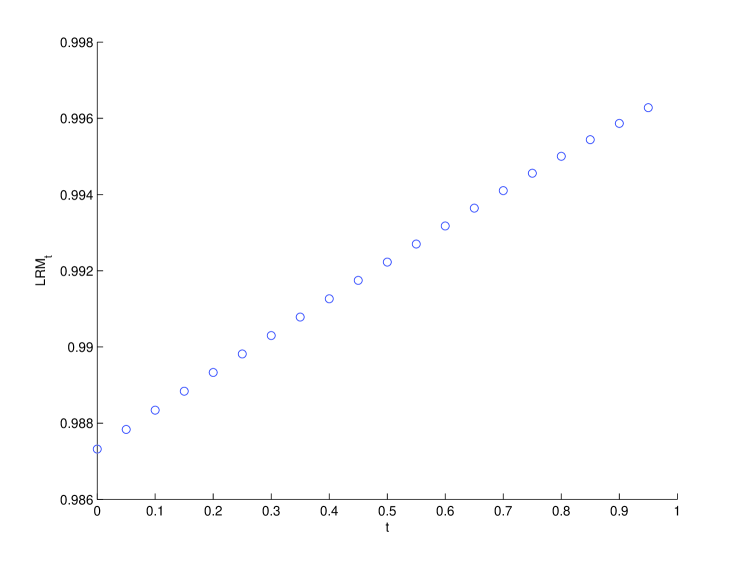
(a) $LRM_{t}$ of a call option with strike price $K=1$ and maturity $T=1$ vs. time for a Merton jump-diffusion model with parameters $\mu=-0.7$, $\sigma=0.2$, $\gamma=1$, $m=0$, and $\delta=1$.

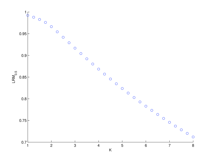
(b) $LRM_{0.5}$ for the same Merton jump-diffusion model as (a) vs. strike price $K$. The vertical axis represents the value of $LRM_{0.5}$

Figure 1: Merton jump-diffusion model

4 Variance Gamma Models

We now consider the case in which $L$ is given as a variance gamma process. Note that $L$ does not have a diffusion component. This means that $\sigma=0$, that is, $I_{1}$ vanishes. A variance gamma process, which has three parameters $\kappa>0$, $m\in{\mathbb{R}}$, and $\delta>0$, is defined as a time-changed Brownian motion with volatility $\delta$, drift $m$, and subordinator $G_{t}$, where $G_{t}$ is a gamma process with parameters $(1/\kappa,1/\kappa)$. In summary, $L$ is represented as

$$L_{t}=mG_{t}+\delta B_{G_{t}}\ \ \mbox{ for }t\in[0,T]\,,$$

where $B$ is a one-dimensional standard Brownian motion. Moreover, the Lévy measure of $L$ is given by

$$\nu(dx)=C(\mathbf{1}_{\{x<0\}}e^{-G|x|}+\mathbf{1}_{\{x>0\}}e^{-M|x|})\frac{dx}{|x|}=C(\mathbf{1}_{\{x<0\}}e^{Gx}+\mathbf{1}_{\{x>0\}}e^{-Mx})\frac{dx}{|x|},$$

where

$$C:=\frac{1}{\kappa},\qquad G:=\frac{1}{\delta^{2}}\sqrt{m^{2}+\frac{2\delta^{2}}{\kappa}}+\frac{m}{\delta^{2}},\qquad M:=\frac{1}{\delta^{2}}\sqrt{m^{2}+\frac{2\delta^{2}}{\kappa}}-\frac{m}{\delta^{2}}.$$

Note that $C$, $G$, and $M$ are positive. To emphasize the parameters, we write $\nu$ with parameters $\kappa$, $m$, and $\delta$ as $\nu(dx)=\nu[\kappa,m,\delta](dx)$. Moreover, by regarding $C$, $G$, and $M$ as parameters, we may express $\nu$ as $\nu(dx)=\nu_{C,G,M}(dx)$. In addition, we assume $M>4$ in this section, which ensures that the first condition of Assumption 1.1 holds, by the following lemma:

Lemma 4.1.

When $M>4$, $\int_{{\mathbb{R}}_{0}}(e^{x}-1)^{n}\nu(dx)<\infty$ for $n=2,4$.

Proof.

For $n=2,4$, we have

$$\int_{1}^{\infty}(e^{x}-1)^{n}\nu(dx) \leq C\int_{1}^{\infty}e^{(n-M)x}dx<\infty\,,$$

$$\int_{0}^{1}(e^{x}-1)^{n}\nu(dx) \leq\int_{0}^{1}x^{n}(e-1)^{n}\nu(dx)\leq C(e-1)^{n}<\infty\,,$$

$$\int_{-1}^{0}(e^{x}-1)^{n}\nu(dx) \leq\int_{-1}^{0}(-x)^{n}\nu(dx)\leq C\int_{-1}^{0}(-x)^{n-1}dx<\infty\,,$$

$$\int_{-\infty}^{-1}(e^{x}-1)^{n}\nu(dx) \leq\int_{-\infty}^{-1}\nu(dx)\leq C\int_{1}^{\infty}e^{-Gx}dx<\infty\,,$$

because $n-M<0$, $0\leq e^{x}-1\leq x(e-1)$ whenever $x\in[0,1]$, $1+x\leq e^{x}$ for any $x\in{\mathbb{R}}$, and $e^{x}\leq 1$ if $x\leq 0$. ∎

Remark 4.2.

We can generalize this lemma to $\int_{{\mathbb{R}}_{0}}|e^{x}-1|^{a}\nu(dx)<\infty$ for any $a\in[1,M)$.

Because $\mu=\int_{{\mathbb{R}}_{0}}x\nu(dx)$, (2) below implies that the second condition of Assumption 1.1 can rewritten as

$$\log\left(\frac{(M-1)(G+1)}{(M-2)(G+2)}\right)>0\geq\log\left(\frac{MG}{(M-1)(G+1)}\right),$$

which is equivalent to $-3<G-M\leq-1$.

4.1 Mathematical preliminaries

The approach to variance gamma models is similar to that in Subsection 3.1. We begin by calculating of $\nu^{{\mathbb{P}}^{\ast}}$.

Proposition 4.3.

$\nu^{{\mathbb{P}}^{\ast}}(dx)=\nu_{(1+h)C,G,M}(dx)+\nu_{-hC,G+1,M-1}(dx)$, where $h=\frac{\mu^{S}}{\int_{{\mathbb{R}}_{0}}(e^{x}-1)^{2}\nu(dx)}$.

Proof.

By the same argument as Proposition 3.1, $\nu^{{\mathbb{P}}^{*}}(dx)=(1+h)\nu(dx)-he^{x}\nu(dx)$. We have $\lambda\nu_{C,G,M}(dx)=\nu_{\lambda C,G,M}(dx)$ for any $\lambda>0$, and

$$e^{x}\nu_{C,G,M}(dx) =e^{x}C(\mathbf{1}_{\{x<0\}}e^{Gx}+\mathbf{1}_{\{x>0\}}e^{-Mx})\frac{dx}{|x|}$$

$$=C(\mathbf{1}_{\{x<0\}}e^{(G+1)x}+\mathbf{1}_{\{x>0\}}e^{-(M-1)x})\frac{dx}{|x|} =\nu_{C,G+1,M-1}(dx)$$

because $M-1>0$. ∎

Remark 4.4.

For any $\lambda>0$, $\lambda\nu[\kappa,m,\delta](dx)$ is a Lévy measure corresponding to the variance gamma process with parameters $\kappa/\lambda$, $\lambda m$, and $\delta\sqrt{\lambda}$. However, $\nu_{C,G+1,M-1}(dx)$ is not necessarily a Lévy measure corresponding to a variance gamma process.

Next we calculate the characteristic function $\phi_{T-t}$ of $L$ under ${\mathbb{P}}^{\ast}$:

Proposition 4.5.

For any $t\in[0,T]$ and $v\in{\mathbb{R}}$, with $\zeta:=v-i\alpha$, we have

$$\phi_{T-t}(\zeta) = \left[\left(1+\frac{i\zeta}{G}\right)\left(1-\frac{i\zeta}{M}\right)\right]^{-(1+h)(T-t)C}\left[\left(1+\frac{i\zeta}{G+1}\right)\left(1-\frac{i\zeta}{M-1}\right)\right]^{h(T-t)C}$$

$$\times\exp\left\{(T-t)i\zeta\left[\mu^{\ast}+(1+h)C\frac{M-G}{GM}-hC\frac{M-G-2}{(G+1)(M-1)}\right]\right\},$$

where $\mu^{\ast}=\int_{{\mathbb{R}}_{0}}(x-e^{x}+1)\nu^{{\mathbb{P}}^{\ast}}(dx)$.

Proof.

First of all, we have

$$\int_{0}^{\infty}(e^{i\zeta x}-1)\frac{e^{-Mx}}{x}\,dx =\int_{0}^{\infty}\frac{e^{-(M-\alpha-iv)x}-e^{-Mx}}{x}\,dx$$

$$=\int_{0}^{\infty}\frac{e^{-(M-\alpha-iv)x}-e^{-(M-\alpha)x}+e^{-(M-\alpha)x}-e^{-Mx}}{x}\,dx$$

$$=i\int_{0}^{\infty}e^{-(M-\alpha)x}\int_{0}^{v}e^{itx}\,dt\,dx+\int_{0}^{\infty}\int_{M-\alpha}^{M}e^{-tx}\,dt\,dx$$

$$=i\int_{0}^{v}\int_{0}^{\infty}e^{-(M-\alpha-it)x}\,dx\,dt+\int_{M-\alpha}^{M}\int_{0}^{\infty}e^{-tx}\,dx\,dt$$

$$=\log\left(\frac{M-\alpha}{M-\alpha-iv}\right)+\log\left(\frac{M}{M-\alpha}\right)=-\log\left(1-\frac{i\zeta}{M}\right),$$ (1)

which provides

$$\int_{{\mathbb{R}}_{0}}(e^{i\zeta x}-1)\nu_{C,G,M}(dx) =C\int_{-\infty}^{0}(e^{i\zeta x}-1)\frac{e^{Gx}}{-x}\,dx+C\int_{0}^{\infty}(e^{i\zeta x}-1)\frac{e^{-Mx}}{x}\,dx$$

$$=-C\left(\log\left(1+\frac{i\zeta}{G}\right)+\log\left(1-\frac{i\zeta}{M}\right)\right).$$

In addition, we have

$$\int_{{\mathbb{R}}_{0}}x\nu_{C,G,M}(dx)=-C\int_{-\infty}^{0}e^{Gx}\,dx+C\int_{0}^{\infty}e^{-Mx}\,dx=-C\frac{M-G}{GM}.$$

Together with Proposition 4.3, we obtain

$$\int_{{\mathbb{R}}_{0}}(e^{i\zeta x}-1-i\zeta x)\nu^{{\mathbb{P}}^{\ast}}(dx) = \log\left(1+\frac{i\zeta}{G}\right)^{-(1+h)C}+\log\left(1-\frac{i\zeta}{M}\right)^{-(1+h)C}$$

$$+\log\left(1+\frac{i\zeta}{G+1}\right)^{hC}+\log\left(1-\frac{i\zeta}{M-1}\right)^{hC}$$

$$+\,i(1+h)C\zeta\frac{M-G}{GM}-ihC\zeta\frac{M-G-2}{(G+1)(M-1)},$$

from which Proposition 4.5 follows. ∎

Now, we reformulate (15) into a linear combination of two Fourier transforms in order to allow use of the FFT. As preparation, we show the following:

Lemma 4.6.

$$\int_{{\mathbb{R}}_{0}}e^{i\zeta x}(e^{x}-1)\nu(dx)=C\log\left(\frac{M-i\zeta}{M-1-i\zeta}\frac{G+i\zeta}{G+1+i\zeta}\right).$$ (2)

Proof.

First of all, we have

$$\int_{{\mathbb{R}}_{0}}e^{i\zeta x}(e^{x}-1)\nu(dx)$$

$$=\int_{{\mathbb{R}}_{0}}e^{(iv+\alpha)x}(e^{x}-1)\nu(dx)$$

$$=C\left\{\int_{0}^{\infty}\frac{1-e^{x}}{x}e^{-(G+\alpha+1+iv)x}\,dx+\int_{0}^{\infty}\frac{e^{x}-1}{x}e^{-(M-\alpha-iv)x}\,dx\right\}.$$ (3)

To calculate (3), we compute

$$\int_{0}^{\infty}\frac{e^{x}-1}{x}e^{-ax}\cos{bx}\,dx\qquad\mbox{ and }\qquad\int_{0}^{\infty}\frac{e^{x}-1}{x}e^{-ax}\sin{bx}\,dx$$

for $a>1$ and $b\in{\mathbb{R}}$. First, we have

$$\int_{0}^{\infty}\frac{e^{x}-1}{x}e^{-ax}\cos{bx}\,dx$$ (4)

$$= \int_{0}^{\infty}\frac{\cos{bx}}{x}\int_{a-1}^{a}xe^{-tx}\,dt\,dx=\int_{a-1}^{a}\int_{0}^{\infty}\cos{bx}\cdot e^{-tx}\,dx\,dt$$

$$= \int_{a-1}^{a}\frac{t}{t^{2}+b^{2}}dt=\frac{1}{2}\log\left(\frac{a^{2}+b^{2}}{(a-1)^{2}+b^{2}}\right).$$

A similar calculation implies that

$$\int_{0}^{\infty}\frac{e^{x}-1}{x}e^{-ax}\sin{bx}\,dx=\int_{a-1}^{a}\frac{b}{t^{2}+b^{2}}\,dt=\tan^{-1}\frac{a}{b}-\tan^{-1}\frac{a-1}{b}.$$ (5)

Noting that $M-\alpha>2$ and $\tan^{-1}x=\frac{i}{2}\log\frac{i+x}{i-x}$ for $x\in{\mathbb{R}}$, we have, by (4) and (5),

$$\int_{0}^{\infty}\frac{e^{x}-1}{x}e^{-(M-\alpha-iv)x}\,dx$$

$$\qquad=\int_{0}^{\infty}\frac{e^{x}-1}{x}e^{-(M-\alpha)x}\cos{vx}\,dx+i\int_{0}^{\infty}\frac{e^{x}-1}{x}e^{-(M-\alpha)x}\sin{vx}\,dx$$

$$\qquad=\frac{1}{2}\log\left(\frac{(M-\alpha)^{2}+v^{2}}{(M-\alpha-1)^{2}+v^{2}}\right)+i\left(\tan^{-1}\frac{M-\alpha}{v}-\tan^{-1}\frac{M-\alpha-1}{v}\right)$$

$$\qquad=\log\left(\frac{M-\alpha-iv}{M-\alpha-1-iv}\right).$$ (6)

Calculating the first term of the right-hand side of (3) in the same way as the above, we obtain

$$\int_{0}^{\infty}\frac{1-e^{x}}{x}e^{-(G+\alpha+1+iv)x}\,dx=\log\left(\frac{G+\alpha+iv}{G+\alpha+1+iv}\right).$$ (7)

Substituting (6) and (7) for (3), we arrive at (2). ∎

From the above lemma, $I_{2}$ is given as follows:

$$\int_{{\mathbb{R}}_{0}}{\mathbb{E}}_{{\mathbb{P}}^{\ast}}[(S_{T}e^{x}-K)^{+}-(S_{T}-K)^{+}\mid{\cal F}_{t-}](e^{x}-1)\nu(dx)$$

$$\qquad= \frac{1}{\pi}\int^{\infty}_{0}K^{-i\zeta+1}\int_{{\mathbb{R}}_{0}}(e^{i\zeta x}-1)(e^{x}-1)\nu(dx)\psi_{2}(\zeta)dv$$

$$\qquad= \frac{1}{\pi}\int^{\infty}_{0}K^{-i\zeta+1}\widetilde{\psi}_{VG}(\zeta)dv-\frac{1}{\pi}\int^{\infty}_{0}C\log\left(\frac{MG}{(M-1)(G+1)}\right)K^{-i\zeta+1}\psi_{2}(\zeta)dv.$$

where

$$\widetilde{\psi}_{VG}(\zeta):=C\log\left(\frac{M-i\zeta}{M-1-i\zeta}\frac{G+i\zeta}{G+1+i\zeta}\right)\psi_{2}(\zeta).$$

Recall that $\psi_{2}(\zeta)=\frac{\phi_{T-t}(\zeta)S_{t-}^{i\zeta}}{(i\zeta-1)i\zeta}$. As a result, we need only use the FFT twice for computing $I_{2}$.

As the final item of this subsection, we estimate a sufficient length for the integration interval of (LABEL:eq-VG-I2) for a given allowable error $\varepsilon>0$ in the sense of (7). We first provide an upper estimate of $\phi_{T-t}$ as follows:

Proposition 4.7.

For any $v\in{\mathbb{R}}$,

$$|\phi_{T-t}(v-i\alpha)|\leq C_{2}|v|^{-2C(T-t)},$$

where

$$C_{2} = (GM)^{(1+h)(T-t)C}[(G+1)(M-1)]^{-h(T-t)C}$$ (9)

$$\times\exp\left\{(T-t)\alpha\left[\mu^{\ast}+(1+h)C\frac{M-G}{GM}-hC\frac{M-G-2}{(G+1)(M-1)}\right]\right\}.$$

Proof.

This can be seen because

$$\left|\left(1+\frac{iv+\alpha}{G}\right)^{-a}\right|\leq\frac{G^{a}}{|v|^{a}}$$

for any $a>0$. ∎

We need to prepare one more lemma:

Lemma 4.8.

$$\left|\int_{{\mathbb{R}}_{0}}e^{i\zeta x}(e^{x}-1)\nu(dx)\right|\leq C\left\{\frac{1}{G+\alpha}+\frac{1}{M-\alpha-1}\right\}.$$ (10)

Proof.

The same sort of calculations as in (1) imply

$$\left|\int_{{\mathbb{R}}_{0}}e^{i\zeta x}(e^{x}-1)\nu(dx)\right|$$

$$\qquad\leq C\left\{\left|\int_{0}^{\infty}\frac{1-e^{x}}{x}e^{-(G+\alpha+1+iv)x}\,dx\right|+\left|\int_{0}^{\infty}\frac{e^{x}-1}{x}e^{-(M-\alpha-iv)x}\,dx\right|\right\}$$

$$\qquad\leq C\left\{\int_{0}^{\infty}\frac{e^{x}-1}{x}e^{-(G+\alpha+1)x}\,dx+\int_{0}^{\infty}\frac{e^{x}-1}{x}e^{-(M-\alpha)x}\,dx\right\}$$

$$\qquad= C\left\{\log\left(1+\frac{1}{G+\alpha}\right)+\log\left(1+\frac{1}{M-\alpha-1}\right)\right\}$$

$$\qquad\leq C\left\{\frac{1}{G+\alpha}+\frac{1}{M-\alpha-1}\right\}.$$

∎

When we calculate (LABEL:eq-VG-I2), $N$ and $\eta$ should be taken so that $N\eta$ satisfies (11) below for a given allowable error $\varepsilon>0$.

Proposition 4.9.

Let $\varepsilon>0$. When $a>0$ satisfies

$$\frac{CC_{2}K^{-\alpha+1}S_{t-}^{\alpha}}{\pi\varepsilon(2C(T-t)+1)}\left[\frac{1}{G+\alpha}+\frac{1}{M-\alpha-1}+\left|\log\left(\frac{MG}{(M-1)(G+1)}\right)\right|\right]\leq a^{2C(T-t)+1},$$ (11)

we have

$$\left|\frac{1}{\pi}\int^{\infty}_{a}K^{-i\zeta+1}\int_{{\mathbb{R}}_{0}}(e^{i\zeta x}-1)(e^{x}-1)\nu(dx)\psi_{2}(\zeta)dv\right|<\varepsilon\,,$$ (12)

where $C_{2}$ is defined in (9).

Proof.

By (10), we have

$$\left|\frac{1}{\pi}\int^{\infty}_{a}K^{-i\zeta+1}\int_{{\mathbb{R}}_{0}}(e^{i\zeta x}-1)(e^{x}-1)\nu(dx)\psi_{2}(\zeta)dv\right|$$

$$\leq \frac{1}{\pi}\Bigg{\{}\left|\int^{\infty}_{a}K^{-i\zeta+1}\int_{{\mathbb{R}}_{0}}e^{i\zeta x}(e^{x}-1)\nu(dx)\psi_{2}(\zeta)dv\right|$$

$$+\left|\int^{\infty}_{a}K^{-i\zeta+1}\int_{{\mathbb{R}}_{0}}(e^{x}-1)\nu(dx)\psi_{2}(\zeta)dv\right|\Bigg{\}}$$

$$\leq \frac{1}{\pi}\left\{\int^{\infty}_{a}\left|K^{-i\zeta+1}\right|\left[\left|\int_{{\mathbb{R}}_{0}}e^{i\zeta x}(e^{x}-1)\nu(dx)\right|+\left|\int_{{\mathbb{R}}_{0}}(e^{x}-1)\nu(dx)\right|\right]\left|\psi_{2}(\zeta)\right|dv\right\}$$

$$\leq \frac{1}{\pi}\left\{K^{-\alpha+1}C\left(\frac{1}{G+\alpha}+\frac{1}{M-\alpha-1}+\left|\log\left(\frac{MG}{(M-1)(G+1)}\right)\right|\right)\int_{a}^{\infty}\left|\psi_{2}(\zeta)\right|dv\right\}.$$

Because Proposition 4.7 implies

$$\left|\psi_{2}(\zeta)\right|=\left|\frac{\phi_{T-t}(\zeta)S_{t-}^{i\zeta}}{(i\zeta-1)i\zeta}\right|\leq\frac{1}{v^{2}}C_{2}|v|^{-2C(T-t)}S_{t-}^{\alpha}=C_{2}S_{t-}^{\alpha}|v|^{-2C(T-t)-2},$$

we have, together with (LABEL:eq-prop-VG3-3),

R.H.S. of (12) $$\leq \frac{1}{\pi}CC_{2}K^{-\alpha+1}S_{t-}^{\alpha}\left[\frac{1}{G+\alpha}+\frac{1}{M-\alpha-1}+\left|\log\left(\frac{MG}{(M-1)(G+1)}\right)\right|\right]$$

$$\times\int_{a}^{\infty}|v|^{-2C(T-t)-2}dv$$

$$= \frac{1}{\pi}CC_{2}K^{-\alpha+1}S_{t-}^{\alpha}\left[\frac{1}{G+\alpha}+\frac{1}{M-\alpha-1}+\left|\log\left(\frac{MG}{(M-1)(G+1)}\right)\right|\right]$$

$$\times\frac{a^{-2C(T-t)-1}}{2C(T-t)+1}.$$

∎

4.2 Numerical results

We illustrate our numerical results for a variance gamma model. Choosing the model parameters as $\kappa=0.15$, $m=-0.2$, and $\delta=0.45$, which meet the second condition of Assumption 1.1, we compute $LRM_{t}$ for the same numerical experiments as in Subsection 3.2. Note that $M>4$ is satisfied. Moreover, we also take the same parameters related to the FFT as in Subsection 3.2. $N\eta$ satisfies (11) for any parameter set. The results are shown in Fig. 2. The computation time to obtain Fig. 2(b) was 0.19 s.

In addition, we implemented the same type of numerical experiments as the above based on market data. We used the Nikkei 225 index for March 2014. We need to set the log price $L_{t}:=\log(S_{t}/S_{0})$, where $S_{0}$ is the price on 28 February 2014, which was 14841.07. We estimate the parameters $C$, $G$, and $M$ in Table 1 from the mean, variance, and skewness of the log price by using the generalized method of moments and the Levenberg–Marquardt method.

Table 1: Estimated parameters

C	$2.469395026815120$
G	$23.743109051760964$
M	$24.903251787154687$

Because $G-M\approx-1.16$, this parameter set satisfies Assumption 1.1. We take $T=1$ and $S_{t-}=14841.07$, that is, $L_{t-}=0$. First, fixing the strike price $K=14000$, we compute $LRM_{t}$ for $t=0,0.05,\ldots,0.95$. Next, fixing $t$ to $0.5$, the values of $LRM_{0.5}$ are computed for $K=10000,11000,\dots,20000$. Note that $N\eta$ satisfies (11). The results of the computation are illustrated in Fig. 3.

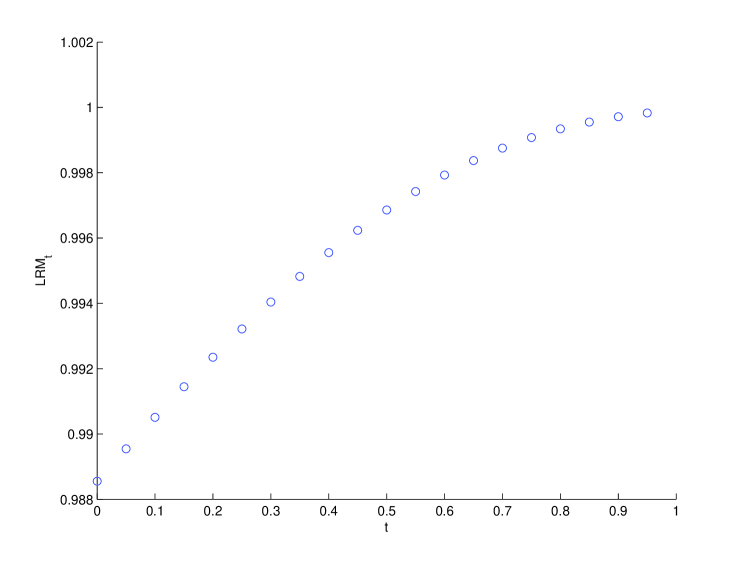
(a) Results of the same numerical experiments as Fig. 1(a) for a variance gamma model with parameters $\kappa=0.15$, $m=-0.2$, and $\delta=0.45$.

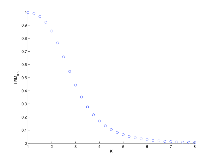
(b) Results for the computation as Fig. 1(b) for the same variance gamma model as in (a).

Figure 2: Variance gamma model with parameters $\kappa=0.15$, $m=-0.2$, $\delta=0.45$

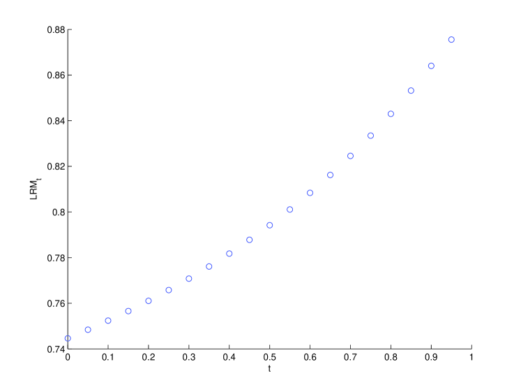
(a) Values of $LRM_{t}$ with strike price $K=14000$ and $S_{t-}=14841.07$ for $t=0,0.05,\ldots,0.95$. The values of the three parameters $C$, $G$, and $M$ are given in Table 1.

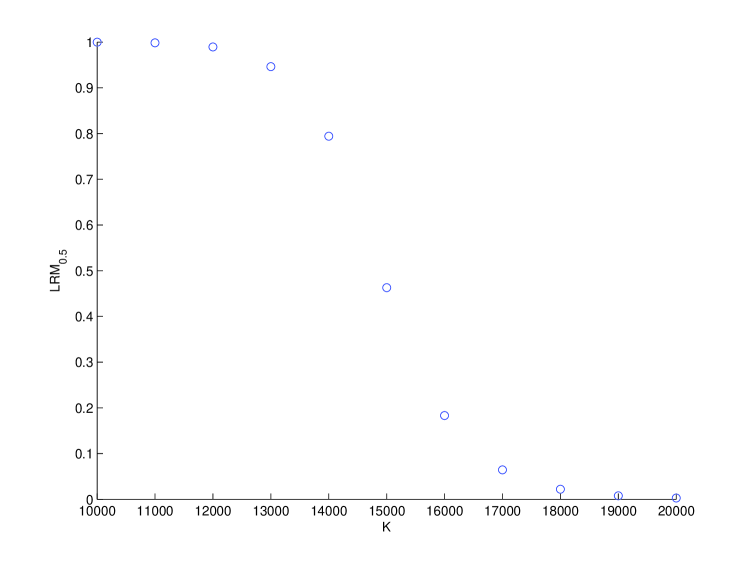
(b) $LRM_{0.5}$ for $K=10000,11000,\dots,20000$ with $S_{0.5}=14841.07$.

Figure 3: Variance gamma model based on the Nikkei 225 index for March 2014

Acknowledgements

Takuji Arai gratefully acknowledges financial support from the Ishii Memorial Securities Research Promotion Foundation.

References

• [1] T. Arai & R. Suzuki (2015) Local risk-minimization for Lévy markets. International Journal of Financial Engineering, in press.
• [2] G. Bertoin (1998) Lévy processes. Cambridge: Cambridge University Press.
• [3] D. Bonetti, D. Leão, A. Ohashi & V. Siqueira (2015) A general multidimensional Monte Carlo approach for dynamic hedging under stochastic volatility, International Journal of Stochastic Analysis 2015, Article ID 863165.
• [4] P. Carr & D. Madan (1999) Option valuation using the fast Fourier transform, Journal of Computational Finance 2 (4), 61–73.
• [5] R. Cont & P. Tankov (2004) Financial Modelling with Jump Processes. Chapman & Hall, London.
• [6] J. W. Cooley & J. W. Tukey (1965) An algorithm for the machine calculation of complex Fourier series, Mathematics of Computation 19, 297–30.
• [7] C.O. Ewald, R. Nawar & T. K. Siu (2013) Minimal variance hedging of natural gas derivatives in exponential Lévy models: theory and empirical performance, Energy Economics 36, 97–107.
• [8] W. Kang & K. Lee (2014) Information on jump sizes and hedging, Stochastics 86, 889–905.
• [9] A. Kélani & F. Quittard-Pinon (2014) Pricing, hedging and assessing risk in a general Lévy context, Bankers, Markets & Investors 131, 30–42.
• [10] K. Lee & S. Song (2007) Insiders’ hedging in a jump diffusion model, Quantitative Finance 7, 537–545.
• [11] P. Leoni, N. Vandaele & M. Vanmaele (2014) Hedging strategies for energy derivatives, Quantitative Finance 14, 1725–1737.
• [12] D. B. Madan & E. Seneta (1987) Chebyshev Polynomial Approximations for Characteristic Function Estimation, Journal of the Royal Statistical Society: Series B (Statistical Methodology)49 (2), 163–169.
• [13] D. B. Madan, P. Carr & E. Chung (1998) The variance gamma process and option pricing, European Finance Review 2, 79–105.
• [14] R. Merton (1976) Option pricing when underlying stock returns are discontinuous, Journal of Financial Economics 3, 125–144.
• [15] W. Schoutens (2003) Lévy Processes in Finance: Pricing Financial Derivatives, John Wiley & Sons, Hoboken.
• [16] M. Schweizer (2001) A Guided Tour through Quadratic Hedging Approaches. In: Handbooks in Mathematical Finance: Option Pricing, Interest Rates and Risk Management ( E. Jouini, J. Cvitanic & M. Musiela eds.), 538–574. Cambridge: Cambridge University Press.
• [17] M. Schweizer (2008) Local Risk-Minimization for Multidimensional Assets and Payment Streams, Banach Center Publications 83, 213–229.
• [18] R. Situ (2005) Theory of Stochastic Differential Equations with Jumps and Applications, Mathematical and Analytical Techniques with Applications to Engineering, Berlin: Springer.
• [19] J. L. Solé, F. Utzet, J. Vives (2007) Canonical Lévy process and Malliavin calculus, Stochastic Processes and their Applications 117, 165–187.
• [20] P. Tankov, (2010) Pricing and hedging in exponential Lévy models: Review of recent results. In: Paris-Princeton Lectures on Mathematical Finance 2010 (R.A. Carmona, E. Cinlar, I. Ekeland, E. Jouini, J.A. Scheinkman & A.N. Touzi Eds.), 319–359, Berlin: Springer.
• [21] Z. Yang, C.O. Ewald & K.R. Schenk-Hoppé (2010) An explicit expression to the locally R-minimizing hedge of a European call in the Hull and White model, Quantitative and Qualitative Analysis in Social Sciences 4, 1–18.