Tunable photon blockade in a hybrid system consisting of an optomechanical device coupled to a two-level system

Abstract

We study photon blockade and anti-bunching in the cavity of an optomechanical system in which the mechanical resonator is coupled to a two-level system (TLS). In particular, we analyze the effects of the coupling strength (to the mechanical mode), transition frequency, and decay rate of TLS on the photon blockade. The statistical properties of the cavity field are affected by the TLS, because the TLS changes the energy-level structure of the optomechanical system via dressed states formed by the TLS and the mechanical resonator. We find that the photon blockade and tunneling can be significantly changed by the transition frequency of the TLS and the coupling strength between the TLS and the mechanical resonator. Therefore, our study provides a method to tune the photon blockade and tunneling using a controllable TLS.

I Introduction

Cavity optomechanics has attracted extensive theoretical and experimental research activity in the last decade Marquardt ; Aspelmeyer ; PR1 ; PR2 ; review1 ; Schwab1 ; Schwab2 ; Painter ; Meystre ; Tang1 ; Tang2 ; NatureMilestones ; Xin . It ranges from testing fundamental aspects of quantum physics and gravity to applications in quantum engineering, quantum measurements Braginsky92 and weak-force detection Caves ; Bocko96 ; Buks06 . For example, experiments OConnell10 have demonstrated the quantum ground state and single-phonon control in a mechanical resonator, which is coupled to a superconducting TLS. It has also been shown that the mechanical resonator can be used for frequency conversion Lin11 ; Hill ; Bochmann ; Lin12 ; Lin13 . By controlling the frequency and the time intervals of a pumping field, nonclassical states of the mechanical motion can be prepared by carrier and sideband transition processes xu-phonon1 ; xu-phonon2 ; Long .

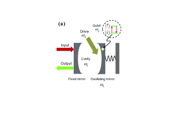
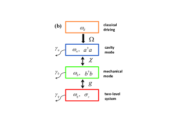
Figure 1: (Color online) (a) Schematic diagram of a hybrid structure consisting of a TLS coupled to the mechanical resonator of an optomechanical system. The TLS (within the black dashed circle) is denoted by a yellow dot inside the oscillating mirror represented by a black spring. Here, $|\downarrow\rangle$ and $|\uparrow\rangle$ denote the ground state and excited state, respectively, of the TLS. The parameters $\omega_{q}$, $\omega_{a}$, $\omega_{b}$, and $\omega_{d}$ denote the frequencies of the TLS, cavity field, oscillating mirror, and driving field, respectively. (b) A schematic diagram for the couplings in the hybrid system with dissipation. The TLS is coupled to the mechanical resonator by the Rabi-type with the coupling strength $g$, the mechanical resonator is coupled to the cavity field with coupling strength $\chi$, and the cavity field is driven by an external field with amplitude $\Omega$. Here, $a$ ($a^{\dagger}$) and $b$ ($b^{\dagger}$) are the annihilation (creation) operators of the cavity mode and mechanical resonator, respectively, and $\sigma_{x}=\sigma_{+}+\sigma_{-}$. $\gamma_{a}$, $\gamma_{b}$, and $\gamma_{q}$ denote the decay rates of the cavity field, the mechanical resonator and the TLS, respectively.

It is known that photon control can be realized in optomechanical systems via an analogue of electromagnetically induced transparency (EIT), well-known in quantum optics. For instance, it has been found that EIT and photon scattering can be used to tune photon transmission in optomechanical systems Agarwal ; Weis ; Liao1 ; Ma ; Qi ; Akram3 . A TLS coupled to the cavity field of an optomechanical system can affect the photon transmission and lead to nonclassical effects for the cavity field Pirkkalainen ; Ciuti ; Jia ; Akram1 ; Akram2 . When the TLS is a controllable superconducting qubit, we find that the EIT window of the optomechanical system can be changed by the superconducting qubit, or, in other words, that the mechanical resonator can affect the absorption and dispersion of the circuit QED system hui . Moreover, the mechanical resonator of an optomechanical system can also interact with a TLS ZLXiang , which can affect the ground state cooling of the mechanical resonator Tdefects , the nonlinearity of the cavity field hybrid2 , and so on. When the cavity field in such a hybrid system is driven by a strong classical field and a weak probe field, the splitting of the phonon energy levels leads to two-color EIT windows Wang , which can be switched to a single one by adjusting the transition frequency of the TLS.

Photon control in an optomechanical system can also be realized via photon blockade and tunneling, which result from the nonlinearity of the cavity field. Photon blockade prevents subsequent photons from resonantly entering the cavity, while the photon-induced tunneling increases the probability of subsequent photons entering the cavity. Thus, photon blockade corresponds to a single-photon transition process, while photon tunneling corresponds to two-photon or multi-photon transition processes. If an optomechanical system coupled to a TLS via a mechanical resonator, both the mechanical resonator and the TLS can induce a nonlinearity in the cavity field, and thus they can be used to realize photon blockade and tunneling. Photon blockade has been studied in various systems, e.g., cavity QED Tian92 ; Leonski94 ; Miran96 ; Imamoglu97 ; Rebic99 ; Kim99 ; Rebic02 ; Smolyaninov02 ; Birnbaum05 , circuit QED Hoffman11 ; Lang11 ; Didier11 ; Liu14 , and optomechanical devices Rabl ; Nunnenkamp11 ; Liao13 . In addition to the single-photon blockade, multiphoton blockade was also studied theoretically (see, e.g., Adam13 ; Adam14a ; Adam14b ; Hovsepyan14 and references therein) and even observed experimentally Smolyaninov02 ; Faraon08 ; Majumdar12 ; Schuster08 ; Kubanek08 . However, to our knowledge, there is no study on how to control photon blockade and tunneling.

In this paper, we study a method to tune photon blockade and anti-bunching in an optomechanical system via a TLS which is coupled to the mechanical resonator of the optomechanical device. In such a hybrid system hybrid2 , the dressed states formed by the mechanical resonator and the TLS affect the photon and phonon blockade of the optomechanical system. It is known that the eigenstates of phonons in an optomechanical devices are described by displaced Fock states Rabl due to the phonon-photon coupling via the radiation pressure. Therefore, the dressed states in the hybrid system should be more complicated, because they formed by the displaced phonon states of the mechanical resonator and the TLS alsing1 ; Kim . If the mechanical mode and the TLS are in the ultrastrong coupling regime, the rotating wave approximation (RWA) doesn’t work, the Rabi type interaction should be considered. In particular, the effect of strong and ultrastrong coupling on the photon blockade is analyzed in many systems Cao ; Zueco ; Niemczyk ; Crisp .

The model studied here is a combination of the usual prototype optomechanical models. Hybrid systems composed of a TLS coupled to the cavity field of an optomechanical system have been studied widely (see, e.g., the recent Refs. Pirkkalainen ; Ciuti ; Jia ; Akram1 ; Akram2 ; Wang and references therein). Specifically, we consider a standard Hamiltonian for two interacting oscillators (i.e., optical and mechanical resonators) in which the mechanical oscillator interacts also with a two-level system (TLS). It is worth noting that the model studied here is nontrivial because the couplings between its constituent subsystems are nonlinear. For example, the interaction between the two oscillators is proportional to the photon number and the position of a mechanical resonator. This nonlinear interactions can induce nonlinearity of the oscillators. For example, as will be shown below, the optical oscillator, due to its interaction with the mechanical oscillator, can be effectively described by a Kerr-type nonlinearity. It is known that the standard Kerr nonlinearity can induce various nonclassical effects Tanas03 ; HarocheBook . These include self-squeezing Tanas83 ; Milburn86 ; Yamamoto86 ; Tanas91 , generation of two-component Yurke86 ; Milburn86 ; Tombesi87 and multi-component Miran90 ; Kirchmair13 Schrödinger cat states, and photon antibunching (if the nonlinearity is driven). The latter is a signature of photon blockade (also referred to as optical state truncation) Tian92 ; Leonski94 ; Imamoglu97 , as also studied here.

The creation of photons due to the mechanical resonator (i.e., oscillating mirror, which causes time-dependent variations of the geometry of our mesoscopic optomechanical system) can be interpreted as a result of the dynamical Casimir effect (DCE), which is also known as non-stationary Casimir effect or motion-induced radiation (from a dynamically deforming mirror). As explained in Ref. Dodonov11 : “The term ‘dynamical Casimir effect’ is used nowadays for a rather wide group of phenomena whose common feature is the creation of quanta (photons) from the initial vacuum (or some other) state of some field (electromagnetic field in the majority of cases) due to time-dependent variations of the geometry (dimensions) or material properties (e.g., the dielectric constant or conductivity) of some macroscopic system.” Specifically, we can interpret the occurrence of photon blockade in the studied system as follows: As mentioned above, the nonlinear interaction between the mechanical and optical resonators of our system can induce an effective Kerr-type nonlinearity of the optical resonator. This driven Kerr nonlinearity can result in photon blockade. Note that this driving is applied directly via the coupling of the mechanical and optical resonators (being related to the DCE) and indirectly via the coupling of the mechanical resonator with the TLS.

The DCE was studied in analogous systems in a number of recent works (see, e.g., Refs. Dodonov10 ; J1 ; J2 ; Wilson11 ; Dodonov11 ; Dodonov12a ; Dodonov12b ). In particular, Ref. Dodonov11 analyzed strong modifications of the cavity field statistics in the DCE due to the interaction with TLSs. Here, we study the effect of a single TLS on photon blockade. The light generated via the DCE can exhibit various nonclassical properties Dodonov10 including squeezing J1 ; J2 ; Wilson11 ; Dodonov97 ; Dodonov00 .

The paper is organized as follows: In Sec. II, we describe the theoretical model. In Sec. III, we write down the master equation and derive the analytical solution in the weak-pumping limit. The photon blockade is analyzed via the second-order degree of coherence in Sec. IV. We finally summarize our results in Sec. V.

II Energy level structure of the hybrid system

II.1 Theoretical model

As schematically shown in Fig. 1, we study a hybrid system which consists of an optomechanical cavity coupled to a TLS with its mechanical mode. We assume that there is no direct coupling between the TLS and the cavity field of the optomechanical part. In this case, the Hamiltonian of the hybrid system can be written as

$$H_{0} = \hbar\omega_{a}a^{{\dagger}}a+\hbar\omega_{b}b^{\dagger}b+\frac{\hbar}{2}\omega_{q}\sigma_{z}-\hbar\chi a^{{\dagger}}a\left(b^{\dagger}+b\right)$$ (1)

$$+\hbar g\left(b^{\dagger}+b\right)\sigma_{x}.$$

Here, $a$ ($a^{\dagger}$) and $b$ ($b^{\dagger}$) are the annihilation (creation) operators of the cavity field and the mechanical resonator, respectively. The frequencies of the cavity field and the mechanical resonator are denoted by $\omega_{a}$ and $\omega_{b}$, respectively. The transition frequency of the TLS is $\omega_{q}$. The Pauli operators $\sigma_{z}$ and $\sigma_{x}$ are used to describe the TLS with the ladder operators $\sigma_{\pm}$ defined by $\sigma_{x}=\sigma_{+}+\sigma_{-}$. The coupling strength between the cavity field and the mechanical resonator is $\chi$, and the parameter $g$ describes the coupling strength between the mechanical resonator and the TLS.

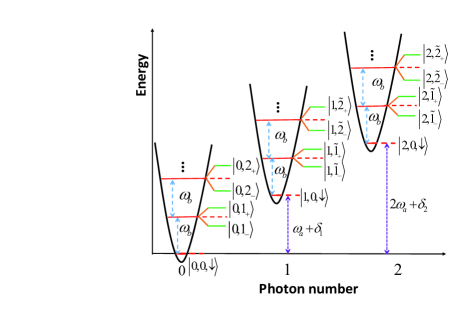
Figure 2: (Color online) Schematic diagram of the energy levels of the hybrid system when the TLS resonantly interacts with the mechanical resonator (the ground state energy of the TLS is assumed to be $0$). Here $|n\rangle$ ($n=0,1,2,\cdot\cdot\cdot$) represent the Fock states of the photons. If the photon number is zero, the dressed states of the phonon and the TLS are: $|1_{\pm}\rangle=|1,\downarrow\rangle\pm|0,\uparrow\rangle$ and $|2_{\pm}\rangle=|2,\downarrow\rangle\pm|1,\uparrow\rangle$. Here $|\uparrow\rangle$ and $|\downarrow\rangle$ denote the eigenstates of the TLS which is not coupled to mechanical resonator. When the photon number is nonzero, the expressions of the wave functions for the dressed states are given by $|\tilde{m}_{\pm}(n)\rangle$ in Eq. (5) ($n,m=0,1,2,\cdot\cdot\cdot$), and the corresponding eigenvalues are given in Eq. (4) (in the stable regime). Here $\delta_{1}=\Delta^{\prime}(1)-\Delta_{0}$ and $\delta_{2}=\Delta^{\prime}(2)-4\Delta_{0}$, where $\Delta^{\prime}(n)=2g\chi\langle\sigma_{x}\rangle/\omega_{b}$ and $\Delta_{0}=\chi^{2}/\omega_{b}$.

It has been shown (e.g., in Ref. xu-phonon1 ) that the mechanical resonator can mediate a Kerr nonlinear interaction between photons of the cavity field in an optomechanical system. Thus, when the mechanical resonator is coupled to the TLS, the mechanical resonator will induce the effect of the TLS on the nonlinearity of the cavity field. To see this clearly, we apply a unitary transformation, $U=\exp{[-\chi a^{\dagger}a(b^{\dagger}-b)/\omega_{b}]}$, to Eq. (1). Then the total Hamiltonian in Eq. (1) becomes

$$H^{\prime}_{0} = \hbar\omega_{a}a^{{\dagger}}a+\hbar\frac{2g\chi}{\omega_{b}}\sigma_{x}a^{{\dagger}}a+\frac{\hbar}{2}\omega_{q}\sigma_{z}+\hbar\omega_{b}b^{\dagger}b$$ (2)

$$-\hbar\frac{\chi^{2}}{\omega_{b}}a^{\dagger}aa^{\dagger}a+\hbar g\left(b^{\dagger}+b\right)\sigma_{x}.$$

Besides the energy level shift $-n^{2}\chi^{2}/\omega_{b}$ ($n=0,1,2,\cdot\cdot\cdot$) induced by the mechanical resonator with the photon number $n$, the interaction between the TLS and the cavity field through $\hbar 2g\chi\sigma_{x}a^{{\dagger}}a/\omega_{b}$ also leads to a photon energy level shift $2g\chi\langle\sigma_{x}\rangle/\omega_{b}$, which is twice the result found with the RWA Wang . This interaction induces a new nonlinearity of the cavity field. For example, in the case of large detuning between the cavity field and the TLS, the TLS can induce another photon-photon Kerr interaction term liuphonon . If we define $\Delta_{0}=\chi^{2}/\omega_{b}$ as the photon nonlinearity induced by the mechanical resonator in the optomechanical system, then the total photon energy levels shifts for the one-photon and two-photon states of the hybrid system are $\delta_{1}=\Delta^{\prime}(1)-\Delta_{0}$, and $\delta_{2}=\Delta^{\prime}(2)-4\Delta_{0}$, respectively, as schematically shown in Fig. 2. Here, both $\Delta^{\prime}(n)=2g\chi\langle\sigma_{x}\rangle/\omega_{b}$ and $\langle\sigma_{x}\rangle$ depend on the photon number $n$ Wang .

II.2 Eigenvalues and eigenstates

We now analyze the eigenvalues and eigenstates of the system when the cavity field of the optomechanical system is in a Fock state $|n\rangle$ with the photon number $n$. In this case, the quantity $\chi n$ can be considered as an effective driving field for the coupled system of the mechanical resonator and the TLS, and the effective Hamiltonian of the mechanical resonator and the TLS for the photon Fock state $|n\rangle$ can be given, from Eq. (1), as

$$H_{b}=\hbar\omega_{b}b^{\dagger}b+\frac{\hbar}{2}\omega_{q}\sigma_{z}+\hbar g\left(b^{\dagger}+b\right)\sigma_{x}-\hbar\chi n\left(b^{\dagger}+b\right),$$ (3)

where the constant term $\hbar\omega_{a}n$ has been neglected.

Let us first study the eigenvalues and eigenstates when the mechanical resonator and the TLS satisfy the resonant interaction condition in Eq. (4), i.e. $\Delta_{d}=\omega_{b}-\omega_{q}=0$. Under the RWA, the dressed state energy levels in the interaction picture can be given as alsing1 ,

$$E_{n,m,\pm} = \pm\hbar\sqrt{m}g\left[1-\left(\frac{2\chi n}{g}\right)^{2}\right]^{3/4}.$$ (4)

Here, $m$ ($m=1,2,\ldots$) denotes the phonon number. If the effective driving field is not very strong, that is, $2\chi n<g$, the dressed states will be stable. Otherwise the phonons have large chances to transit to high energy levels and the dressed states will be unstable alsing1 ; Kim . The energy levels of the dressed states are also functions of the photon number. The dressed states are always stable for the $0$ photon state, however, the dressed states become unstable when $n>g/(2\chi)$. We can see from Eq. (4) that each energy level has an extra term compared with $\pm\hbar\sqrt{m}g$ of the common dressed states in the resonant interaction between the TLS and the mechanical resonator. Here, the splitting width of the dressed states is affected by the quantum states of both photons and phonons.

If the photon number is zero, the eigenvalues corresponding to the dressed states in Eq. (4) become $\pm\hbar\sqrt{m}g$, and the corresponding dressed states can be written as $|m_{\pm}\rangle=\left[|m,\downarrow\rangle\pm|m-1,\uparrow\rangle\right]/\sqrt{2}$, which are the common dressed states of the resonant interaction between the TLS and the mechanical resonator, as schematically shown in Fig. 2. The dressed states, corresponding to the eigenvalues in Eq. (4), can be written as alsing1 ,

$$|\tilde{m}_{\pm}(n)\rangle = \frac{1}{\sqrt{2}}\left[|\eta,\beta(E_{n,m,\pm});m-1\rangle|P\rangle\right.$$ (5)

$$\left.\pm i|\eta,\beta(E_{n,m,\pm});m\rangle|M\rangle\right].$$

Here $|P\rangle$ and $|M\rangle$ correspond to quantum states of the TLS, and the expression of $|P\rangle$ is given by

$$|P\rangle = \frac{1}{\sqrt{2}}\left[\left(1+\sqrt{\varepsilon}\right)^{1/2}|\uparrow\rangle-\left(1-\sqrt{\varepsilon}\right)^{1/2}|\downarrow\rangle\right],$$ (6)

with $\varepsilon=1-\left(2\chi n/g\right)^{2}$. The expression of $|M\rangle$ can be obtained by replacing $|\uparrow\rangle$ and $|\downarrow\rangle$ with $|\downarrow\rangle$ and $|\uparrow\rangle$ in Eq. (6). The state $|\eta;\beta;m\rangle$ in Eq. (5) is given as

$$|\eta;\beta;m\rangle=D(\beta)S(\eta)|m\rangle.$$ (7)

The squeezing operator in Eq. (7) is defined as $S(\eta)=\exp{[\frac{1}{2}(\eta b^{\dagger 2}-\eta^{\ast}b^{2})]}$, while the expression of the displacement operator is $D(\beta)=\exp{(\beta b^{\dagger}-\beta^{\ast}b)}$. The parameters $\beta$ and $\eta$ are defined as $\beta(E)=2i\chi nE/\left(\hbar g^{2}\varepsilon\right)$, $\eta=r$, and $\exp{(2r)}=\sqrt{\varepsilon}$. We can find that the dressed states in the hybrid system are formed by the superposition states $|P\rangle$ and $|M\rangle$ of the TLS, not the eigenstates $|\uparrow\rangle$ or $|\downarrow\rangle$ as in common dressed states. This leads to more complicated phenomena when a probe field passes through such a system. If the mechanical resonator and the TLS are in the large detuning regime, the energy level spacing between two dressed states becomes larger alsing1 .

In circuit QED, the standard photon blockade is significantly changed by the ultrastrong coupling between the cavity field and the TLS Hartmann . Since the sideband-transition processes in optomechanics usually accompany the absorption or emission of phonons, the variation of phonon energy levels in a hybrid system can also affect transitions of photons. So we will also study the effect of the ultrastrong coupling between the mechanical resonator and the TLS on the photon blockade in the hybrid devices.

III Master Equation and weak pumping limit

III.1 Master equation

To study photon blockade, we assume that the cavity field of the hybrid system is driven by a classical field with frequency $\omega_{d}$, the coupling strength between the driving field and the cavity field is $|\Omega|$. In the rotating reference frame at the frequency $\omega_{d}$, the Hamiltonian of the driven hybrid system becomes

$$H_{r} = \hbar\Delta_{a}a^{{\dagger}}a+\hbar\omega_{b}b^{\dagger}b+\frac{\hbar}{2}\omega_{q}\sigma_{z}-\hbar\chi a^{{\dagger}}a\left(b^{\dagger}+b\right)$$ (8)

$$+\hbar g\left(b^{\dagger}+b\right)\sigma_{x}+i\hbar\left(\Omega a^{{\dagger}}-\Omega^{\ast}a\right),$$

where $\Delta_{a}=\omega_{a}-\omega_{d}$ describes the detuning between the cavity field and the driving filed.

After introducing the environmental noise, the master equation of the density operator $\rho$ for the driven hybrid system can be given as

$$\dot{\rho}=\frac{i}{\hbar}[\rho,H_{r}]+L_{a}(\rho)+L_{b}(\rho)+L_{\sigma}(\rho).$$ (9)

The Lindblad dissipators for the photons and phonons are given by

$$L_{o}(\rho) = \gamma_{o}n_{o}\left(o\rho o^{\dagger}+o^{\dagger}\rho o-o^{\dagger}o\rho-\rho o^{\dagger}o\right)$$ (10)

$$+\frac{\gamma_{o}}{2}\left(2o\rho o^{\dagger}-o^{\dagger}o\rho-\rho o^{\dagger}o\right),$$

where $o=a$ or $b$ corresponds to the variables of the photon or phonon, respectively. The Lindblad dissipator for the two-level system is

$$L_{\sigma}(\rho) = \gamma_{q}n_{q}\left(\sigma_{-}\rho\sigma_{+}+\sigma_{+}\rho\sigma_{-}-\sigma_{+}\sigma_{-}\rho-\rho\sigma_{+}\sigma_{-}\right)$$ (11)

$$+\frac{\gamma_{q}}{2}\left(2\sigma_{-}\rho\sigma_{+}-\sigma_{+}\sigma_{-}\rho-\rho\sigma_{+}\sigma_{-}\right).$$

This type of master equations was also studied by Kossakowski et al. Kossakowski72 ; Kossakowski76 ; Kossakowski78 . Here $\gamma_{a}$, $\gamma_{b}$, and $\gamma_{q}$ are the decay rates of the photon, the phonon, and the TLS, respectively, while $n_{a}$, $n_{b}$, and $n_{q}$ correspond to thermal fluctuation quantum numbers, with $n_{i}=1/[\exp(\hbar\omega_{i}/(k_{B}T))]$ ($i=a,b,q$) where $k_{B}$ is the Boltzmann constant and $T$ is the temperature. Usually, the thermal photon number $n_{a}$ can be neglected in the low-temperature limit because of the high frequency of the cavity field.

The master equation in Eq. (9) can also be numerically solved in the complete basis $|n,m,z\rangle$ (for $n,m=0,1,2,\ldots$, and $z=\uparrow,\downarrow$) in the case of weak driving field and low temperatures Tan ; J1 ; J2 . Because higher excited states can be neglected in this case, the photon and phonon numbers can be truncated to small values. By numerically solving the master equation, we can obtain $\rho$ which in turn lets us calculate various physical properties of the hybrid system.

III.2 Analytical solutions in the weak-driving limit

If the driving field coupling $\Omega$ is very weak in comparison to the Kerr nonlinearity, and also the temperature is very low, then, due to photon blockade, only lower energy levels of the cavity field and mechanical resonator are occupied. If the photon number $n$ and phonon number $m$ are truncated to $n=2$ and $m=1$, respectively, then the quantum state of the hybrid system can be written by xunwei2 ; Bamba ; Savona

$$|\psi\rangle = C_{00\downarrow}|0,0,\downarrow\rangle+C_{00\uparrow}|0,0,\uparrow\rangle+C_{10\downarrow}|1,0,\downarrow\rangle$$ (12)

$$+C_{10\uparrow}|1,0,\uparrow\rangle+C_{01\downarrow}|0,1,\downarrow\rangle+C_{01\uparrow}|0,1,\uparrow\rangle$$

$$+C_{20\downarrow}|2,0,\downarrow\rangle+C_{20\uparrow}|2,0,\uparrow\rangle+C_{11\downarrow}|1,1,\downarrow\rangle$$

$$+C_{11\uparrow}|1,1,\uparrow\rangle+C_{21\downarrow}|2,1,\downarrow\rangle.$$

The coefficients $C_{nmk}$ (with photon numbers $n=0,1,2$, phonon numbers $m=0,1$, and the eigenvalues $k=\downarrow,\uparrow$ of the dressed TLS states) describe the amplitudes of the corresponding quantum states, and $p_{nmk}=|C_{nmk}|^{2}$ are the corresponding occupation probabilities.

We use the second-order degree of coherence to describe the statistical properties of the cavity field. The equal-time second-order degree of coherence is defined by

$$g^{(2)}(0)=\frac{\langle a^{\dagger}(t)a^{\dagger}(t)a(t)a(t)\rangle}{\langle a^{\dagger}(t)a(t)\rangle^{2}}.$$ (13)

In the weak-driving limit, using Eq. (12) and Eq. (13), the second-order degree of coherence can be approximately given as

$$g^{(2)}(0)\approx\frac{2\left(|C_{20\downarrow}|^{2}+|C_{20\uparrow}|^{2}+|C_{21\downarrow}|^{2}\right)}{(|C_{10\downarrow}|^{2}+|C_{10\uparrow}|^{2}+|C_{11\downarrow}|^{2}+|C_{11\uparrow}|^{2})^{2}}.$$ (14)

The result of Eq. (14) can be used to approximately describe the photon statistical properties in the limit of weak driving and low temperatures. This will be compared with numerical results, calculated using the master equation, in the following sections.

To obtain the coefficients $C_{10\downarrow}$, $C_{10\uparrow}$, $C_{11\downarrow}$, $C_{11\uparrow}$, $C_{20\downarrow}$, $C_{20\uparrow}$, and $C_{21\downarrow}$ in Eq. (12), we solve the Schrödinger equation for the quantum state $|\psi\rangle$ of the hybrid system

$$i\frac{d|\psi\rangle}{dt}=H^{\prime}_{r}|\psi\rangle.$$ (15)

Here, the effective non-Hermitian Hamiltonian

$$H^{\prime}_{r} = \hbar\Delta^{\prime}_{a}a^{{\dagger}}a+\hbar\omega^{\prime}_{m}b^{\dagger}b+\frac{\hbar}{2}\omega^{\prime}_{q}\sigma_{z}-\hbar\chi a^{{\dagger}}a\left(b^{\dagger}+b\right)$$ (16)

$$+\hbar g\left(b^{\dagger}+b\right)\sigma_{x}+i\hbar\left(\Omega a^{{\dagger}}-\Omega^{\ast}a\right),$$

includes dissipations with $\Delta^{\prime}_{a}=\Delta_{a}-i\gamma_{a}/2$, $\omega^{\prime}_{b}=\omega_{b}-i\gamma_{b}/2$, and $\omega^{\prime}_{q}=\omega_{q}-i\gamma_{q}/2$. Here we assume that the thermal fluctuation of the photons, phonons and the TLS can be neglected in the extreme low-temperature limit.

Because we are interested in the statistical properties of the cavity field in the steady state, thus we can set $d|\psi\rangle/dt=0$. By substituting Eqs. (12) and (16) into Eq. (15), we can obtain linear equations, as shown in Eqs. (22)-(31) of the Appendix A. By solving these linear equations, we can obtain the coefficients in Eq. (12), that is,

$$C_{11\downarrow}=i\Omega\eta_{1},~{}~{}~{}C_{11\uparrow}=i\Omega\eta_{2},$$ (17)

$$C_{10\downarrow}=i\Omega\eta_{3},~{}~{}~{}C_{10\uparrow}=i\Omega\eta_{4},$$ (18)

$$C_{20\downarrow}=\Omega^{2}\eta_{5},~{}~{}~{}C_{20\uparrow}=\Omega^{2}\eta_{6},$$ (19)

$$C_{21\downarrow}=\Omega^{2}\eta_{7}.$$ (20)

The expressions of $\eta_{i}(i=1,2,\cdot\cdot\cdot,7)$ can be found in Eqs. (A). In the weak-driving and low-temperature limit, we find that $C_{10\downarrow}$, $C_{10\uparrow}$, $C_{11\downarrow}$, and $C_{11\uparrow}$ are proportional to $\Omega$, while $C_{20\downarrow}$, $C_{20\uparrow}$, and $C_{21\downarrow}$ are proportional to $\Omega^{2}$. The value of $C_{00\downarrow}$ will be close to $1$ and the amplitudes of the excited state tend to $0$ if the value of $\Omega\rightarrow 0$.

IV Photon Blockade

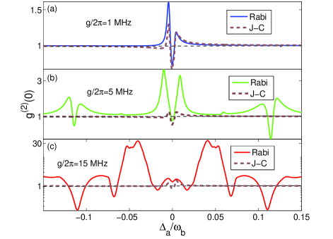
Figure 3: (Color online) Equal-time second-order degree of coherence $g^{(2)}(0)$ as a function of $\Delta_{a}/\omega_{b}=(\omega_{a}-\omega_{d})/\omega_{b}$ in the cavity steady-state limit. The solid curve in each panel is plotted with the Rabi model (without RWA), while the dashed curve is plotted with the Jaynes-Cummings(J-C) model (with RWA). The curves in the three panels correspond to different coupling strengths between the mechanical mode and the TLS: (a) $g/(2\pi)=1$ MHz; (b) $g/(2\pi)=5$ MHz; and (c) $g/(2\pi)=15$ MHz. The other parameters for the three solid curves are: $\omega_{b}/(2\pi)=\omega_{q}/(2\pi)=10$ MHz, $\gamma_{a}/(2\pi)=0.02$ MHz, $\gamma_{b}/(2\pi)=0.001$ MHz, $\gamma_{q}/(2\pi)=0.002$ MHz, $\chi/(2\pi)=0.2$ MHz, $g/(2\pi)=4$ MHz, $T=1$ mK, and $|\Omega|/(2\pi)=0.02$ MHz.

In an optomechanical system, the mechanical resonator leads to the nonlinearity and energy levels shift of the cavity field. For the single-photon state, such shift is $\Delta_{0}=\chi^{2}/\omega_{b}$, while it is $4\Delta_{0}$ for the two-photon state Rabl . Both the photon blockade Rabl and tunneling xunwei1 ; Roque can occur in the strong single-photon optomechanical coupling regime. Besides mechanical mode, the TLS can also lead to the variation of photon energy levels (see Eq. (2)). The energy level structure of the hybrid system becomes very complex since $\langle\sigma_{x}\rangle$ is a complicated function of $\chi$ Wang . The dressed states formed by the TLS and the mechanical mode lead to the splitting of phonon energy levels (in standard optomechanical systems).

We now study how a TLS affects the photon blockade of a hybrid system via the second-order degree of coherence

$$g^{(2)}(0)=\frac{\text{Tr}(\rho a^{\dagger 2}a^{2})}{[\text{Tr}(\rho a^{\dagger}a)]^{2}},$$ (21)

which is calculated here using the master equation in Eq. (9) and will be compared to the result calculated using Eq. (14). The value of $g^{(2)}(0)<1$ ($g^{(2)}(0)>1$) corresponds to sub-Poisson (or super-Poisson) statistics of the cavity field, which is a nonclassical (classical) effect. This effect of the sub-Poisson photon statistics is often referred to as photon antibunching. The dips ( resonant peaks) of $g^{(2)}(0)$ can be used to characterize the photon blockade (tunneling) processes. The photon blockade describes the single-photon transition, while the photon tunneling corresponds to a multi-photon resonant transition.

We plot $g^{(2)}(0)$ as a function of $\Delta_{a}/\omega_{b}$ in Fig. 3 by using the master equation in Eq. (9), the curves in different panels correspond to different values of the coupling strength $g$ between the mechanical mode and the TLS. To further study the effect of the counter-rotating term on the photon blockade, using the master equation in Eq. (9), we compare the numerical results of $g^{(2)}(0)$ with (solid curves) and without (dashed curves) the RWA. The minimum value of $g^{(2)}(0)$ is smaller than $1$ at the dip near $\Delta_{a}/\omega_{b}=0$ in the blue solid curve of Fig. 3(a), so the photon blockade can be observed. If the value of $g$ is much smaller than the transition frequency $\omega_{q}$, the TLS has a small effect on the photon blockade in the blue solid curve of Fig. 3(a) [compare with the black dashed curve in Fig. 5(c)]. If the value of $g$ becomes larger, the TLS leads to two new dips (photon blockade) and several peaks (photon tunneling) in the green solid curve of Fig. 3(b). This results from the counter-terms $(b\sigma^{+}+\sigma_{-}b^{\dagger})$ which can be understood by comparing the green solid and brown dashed curves of Fig. 3(b). When the value of coupling strength $g$ is larger than the transition frequency of the TLS, that is $g>\omega_{q}$, more dips and peaks appear in the red solid curve of Fig. 3(c). And the minimum value of $g^{(2)}(0)$ near $\Delta_{a}/\omega_{b}=0$ is larger than $1$, so the photon blockade in this regime vanishes in ultra-strong coupling regime. Actually, a similar phenomenon of photon blockade in the ultrastrong coupling regime has been studied in circuit QED Hartmann .

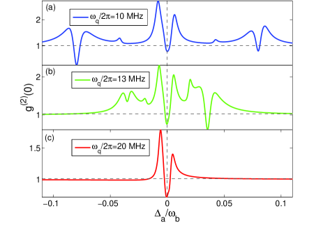
Figure 4: (Color online) Equal-time second-order degree of coherence $g^{(2)}(0)$ as a function of $\Delta_{a}/\omega_{b}=(\omega_{a}-\omega_{d})/\omega_{b}$ in the steady-state limit. The curves in the three panels correspond to different transition frequencies of the TLS: (a) $\omega_{q}/(2\pi)=10$ MHz; (b) $\omega_{q}/(2\pi)=13$ MHz; and (c) $\omega_{q}/(2\pi)=20$ MHz. The other parameters are as in Fig. 3, except $g/(2\pi)=4$ MHz.

Figure 4 describes the effect of the TLS transition frequency on the photon blockade in the hybrid system. The blue solid curve of Fig. 4(a) describes $g^{(2)}(0)$ when the mechanical resonator interacts resonantly with a TLS, while the green solid [in Figs. 4(b)] and red solid curves [in Fig. 4(c)] correspond to the detuning cases. When the mechanical mode and the TLS are in the detuning regime, the positions of the left and right dips (relative to the point $\Delta_{a}/\omega_{b}=0$) are changed in the green solid curve of Fig. 4(b). The minimum value of $g^{(2)}(0)$ of the left dip becomes larger than $1$, so the photon blockade disappears near this point. But the photon blockade near the right dip is enhanced. If the detuning $|\omega_{q}-\omega_{b}|$ is larger than the coupling strength $g$, all the dips and peaks induced by the TLS disappear in the red solid curve of Fig. 4(c), in this case the photon blockade is similar to that of standard optomechanical systems [see the black solid curve in Fig. 5(c)].

The effect of the decay rate $\gamma_{q}$ on the photon blockade of optomechanical systems is discussed in Fig. 5. If the value of $\gamma_{q}$ becomes larger, the dip near $\Delta_{a}/\omega_{b}=0$ is almost invariant, but the left and right dips (relative to the point $\Delta_{a}/\omega_{b}=0$) change greatly. The minimum value of $g^{(2)}(0)$ near the right dip is even larger than $1$, so the photon blockade disappears in this regime. The photon blockade near the left dip will also vanish if the value of $\gamma_{q}$ continues to increase. If the decay rate becomes very large, all the new dips and peaks induced by the TLS vanish, and the photon blockade in the red solid curve of Fig. 5(c) is then almost then same to that of standard optomechanical system [see the black dashed curve in Fig. 5(c)].

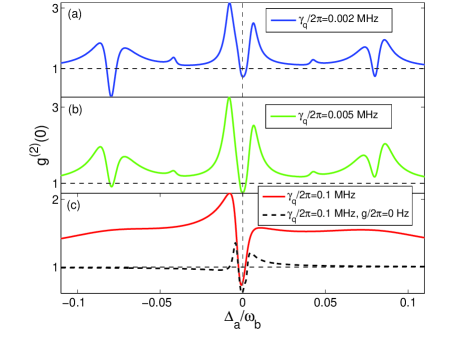
Figure 5: (Color online) Equal-time second-order degree of coherence $g^{(2)}(0)$ as a function of $\Delta_{a}/\omega_{b}=(\omega_{a}-\omega_{d})/\omega_{b}$ in the steady-state limit. The curves in three panels correspond to different decay rates of TLS: (a) $\gamma_{q}/(2\pi)=0.002$ MHz; (b) $\gamma_{q}/(2\pi)=0.005$ MHz; and (c) $\gamma_{q}/(2\pi)=0.1$ MHz. Here $g/(2\pi)=4$ MHz for the solid curves, while $g/(2\pi)=0$ Hz for black dashed curve in panel (c), and the other parameters are same as in Fig. 3.

In Fig. 6, we compare the results obtained numerically by the master equation in Eq. (9) with those obtained analytically in Eq. (14). We plot $g^{(2)}(0)$ as a function of the detuning $\Delta_{a}/\omega_{b}$ for $T=0$ K. The blue solid curves in Figs. 6(a) and 6(b) are plotted using the master equation, while the red dashed curves are plotted with the analytical result in Eq. (14). The results of two methods are almost the same for Fig. 6(a). If the coupling strength $g$ becomes larger, the deviations between the blue solid and red dashed curves in Fig. 6(b) becomes larger. This difference originates from the approximation when Eq. (14) was derived, because, contrary to our precise numerical calculations, we have assumed in our analytical approach that (i) the system evolution is pure and (ii) some transition processes, such as $|0,2,\downarrow\rangle$, $|0,2,\uparrow\rangle$, $|1,2,\downarrow\rangle$, etc., were neglected.

Therefore, we conclude that the coupling strength (to the mechanical mode), transition frequency, and the decay rate of the TLS can be used to tune the photon blockade and tunneling of optomechanical systems.

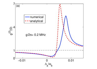
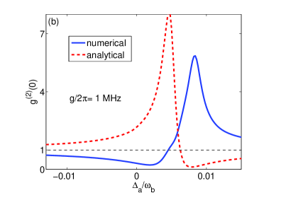
Figure 6: (Color online) Equal-time second-order degree of coherence $g^{(2)}(0)$ as a function of $\Delta_{a}/\omega_{b}$ at zero temperature in the steady-state limit. The blue solid curves correspond to our numerical precise solutions of the master equation, while the red dashed curves are plotted with the analytical result in Eq. (14). Both figures are plotted by substituting $\sigma_{z}$ with $\sigma_{+}\sigma_{-}$ in Eq. (8). Here $\chi/(2\pi)=0.5$ MHz, $|\Omega|/(2\pi)=0.01$ MHz, and $T=0$ K, while other parameters are the same as in Fig. 3.

V Conclusions

We have studied single-photon blockade and tunneling(corresponding to multi-photon blockade) of a hybrid system consisting of an optomechanical cavity and a TLS. We find that the photon blockade of the optomechanical device is significantly affected by a TLS when it is coupled to the mechanical resonator. Compared with the results of only the optomechanical cavity, the TLS shifts and splits the peaks and dips of the second-order degree of coherence of the cavity field in the optomechanical subset. We also find that the TLS gives rise to several new peaks and dips in the second-order degree of coherence of the cavity field in the hybrid system.

If the coupling strength (between the mechanical mode and the TLS) is comparable or larger than the transition frequency of the TLS, new blockade dips and resonant peaks appear for the second degree of coherence. Moreover the new blockade dips and resonant peaks can be tuned if we change the transition frequency or the decay rate of the TLS. The photon anti-bunching of hybrid systems can also be tuned if we change the parameters of the TLS. That is, our study may provide a new method to control and tune the nonlinearity and nonclassical effect of the cavity field of the optomechanical system by coupling to a tunable TLS. Our calculation may also provide an approach to detect a low-frequency TLS (which might be a defect in a mechanical resonator) using optomechanics.

VI Acknowledgement

We thank Anton F. Kockum for valuable suggestions to the manuscript. Hui Wang thanks Nan Yang and Jing Zhang for technical support. Y.X.L. is supported by the National Natural Science Foundation of China under Grant No. 61328502, the National Basic Research Program of China (973 Program) under Grant No. 2014CB921401, the Tsinghua University Initiative Scientific Research Program, and the Tsinghua National Laboratory for Information Science and Technology (TNList) Cross-discipline Foundation. A.M. acknowledges a long-term fellowship from the Japan Society for the Promotion of Science (JSPS). A.M. is supported by the Polish National Science Centre under the grants No. DEC-2011/02/A/ST2/00305 and No. DEC-2011/03/B/ST2/01903. F.N. is partially supported by the RIKEN iTHES Project, the MURI Center for Dynamic Magneto-Optics via the AFOSR award number FA9550-14-1-0040, the IMPACT program of JST, and a Grant-in-Aid for Scientific Research (A).

*

Appendix A The expansion coefficients of Eq. (16)

In the weak pumping limit, only low excited states of photons and phonons are occupied. If the temperature is extremely low, the quantum state of the hybrid system can be written as a sum of the finite orthogonal basis states given in Eq. (12). Considering the effect of environment noises, the effective non-Hermitian Hamiltonian of the hybrid system can be obtained in Eq. (16). In the steady state case, we can set $d|\psi\rangle/dt=0$. Substituting Eqs. (12) and (16) into Eq. (15), we obtain linear equations about the expanding coefficients of Eq. (12) as follow:

$$0 = \left(\omega^{\prime}_{q}/2\right)C_{00\uparrow}+gC_{01\downarrow}-i\Omega^{\ast}C_{10\uparrow},$$ (22)

$$0 = \Delta^{-}_{1}C_{01\downarrow}+gC_{00\uparrow}-i\Omega^{\ast}C_{11\downarrow},$$ (23)

$$0 = \Delta^{+}_{1}C_{01\uparrow}+gC_{00\downarrow}-i\Omega^{\ast}C_{11\uparrow},$$ (24)

$$0 = \Delta^{-}_{2}C_{10\downarrow}-\chi C_{11\downarrow}+gC_{11\uparrow}+i\Omega C_{00\downarrow}$$ (25)

$$-i\sqrt{2}\Omega^{\ast}C_{20\downarrow},$$

$$0 = \Delta^{+}_{2}C_{10\uparrow}-\chi C_{11\uparrow}+gC_{11\downarrow}+i\Omega C_{00\uparrow}$$ (26)

$$-i\sqrt{2}\Omega^{\ast}C_{20\uparrow},,$$

$$0 = \Delta^{-}_{3}C_{11\downarrow}-\chi C_{10\downarrow}+gC_{10\uparrow}+i\Omega C_{01\downarrow}$$ (27)

$$-i\sqrt{2}\Omega^{\ast}C_{21\downarrow},,$$

$$0 = \Delta^{+}_{3}C_{11\uparrow}-\chi C_{10\uparrow}+gC_{10\downarrow}+i\Omega C_{01\uparrow},$$ (28)

$$0 = \Delta^{-}_{4}C_{20\downarrow}-2\chi C_{21\downarrow}+i\sqrt{2}\Omega C_{10\downarrow},$$ (29)

$$0 = \Delta^{+}_{4}C_{20\uparrow}+gC_{21\downarrow}+i\sqrt{2}\Omega C_{10\uparrow},$$ (30)

$$0 = \Delta_{5}C_{21\downarrow}-2\chi C_{20\downarrow}+gC_{20\uparrow}+i\sqrt{2}\Omega C_{11\downarrow},$$ (31)

with the definitions of $\Delta_{i}(i=1,2,\ldots,9)$ being

$$\Delta^{\mp}_{1} = \omega^{\prime}_{m}\mp\omega^{\prime}_{q}/2,$$

$$\Delta^{\mp}_{2} = \Delta^{\prime}_{a}\mp\omega^{\prime}_{q}/2,$$

$$\Delta^{\mp}_{3} = \Delta^{\prime}_{a}+\omega^{\prime}_{m}\mp\omega^{\prime}_{q}/2,$$

$$\Delta^{\mp}_{4} = 2\Delta^{\prime}_{a}\mp\omega^{\prime}_{q}/2,$$

$$\Delta_{5} = 2\Delta^{\prime}_{a}+\omega^{\prime}_{m}-\omega^{\prime}_{q}/2.$$ (32)

The equation $0=-\omega^{\prime}_{q}C_{00\downarrow}/2-i\Omega^{\ast}C_{10\downarrow}$ has no physical meaning if $|\Omega|\longrightarrow 0$, so it can be neglected. The system has a probability to remain in the ground state $|0,0,\downarrow\rangle$ in the weak-pumping limit, so we can set $C_{00\downarrow}=1$ (then the expansion coefficients are unnormalized). The terms $(i\sqrt{2}\Omega^{\ast}C_{20\downarrow})$ in Eq. (25), $(i\Omega^{\ast}C_{20\uparrow})$ in Eq. (26), and $(-i\sqrt{2}\Omega^{\ast}C_{21\downarrow})$ in Eq. (27) are of higher-order in $\Omega$, so they can be neglected.

Through some calculations, we can obtain the solutions of the expansion coefficients in Eq. (12). The corresponding coefficients $\eta_{i}(i=1,2,\ldots,7)$ are given by

$$\eta_{1} = \left(\chi\Delta^{+}_{1}\lambda_{11}+g\Delta^{+}_{1}\lambda_{9}-\Delta^{-}_{2}g\lambda_{9}\right)/D_{1},$$

$$\eta_{2} = -\left(g\Delta^{+}_{1}\lambda_{8}+g\Delta^{-}_{2}\lambda_{8}+\chi\Delta^{+}_{1}\lambda_{10}\right)/D_{1},$$

$$\eta_{3} = \left(\chi\eta_{1}-g\eta_{2}-1\right)/\Delta^{-}_{2},$$

$$\eta_{4} = \left(\chi\eta_{2}-\lambda_{4}\eta_{1}\right)/\lambda_{3},$$

$$\eta_{5} = \left(\lambda_{13}\lambda_{14}+2\chi g\lambda_{15}\right)/D_{2},$$

$$\eta_{6} = -\left(\lambda_{12}\lambda_{15}+2\chi g\lambda_{14}\right)/D_{2},$$

$$\eta_{7} = 2\chi\left(\lambda_{13}\lambda_{14}+2\chi g\lambda_{15}\right)/(\Delta_{5}D_{2})+\sqrt{2}\eta_{1}/\Delta_{5}$$ (33)

$$+g\left(\lambda_{12}\lambda_{15}+2\chi g\lambda_{14}\right)/(\Delta_{5}D_{2}),$$

with $D_{1}=\Delta^{+}_{1}\Delta^{-}_{2}\left(\lambda_{9}\lambda_{10}-\lambda_{8}\lambda_{11}\right)$ and $D_{2}=\lambda_{12}\lambda_{13}-4\chi^{2}g^{2}$. The parameters $\lambda_{i}(i=1,2,\ldots,15)$ in the above equations are

$$\lambda_{1} = \Delta^{-}_{1}-2g^{2}/\omega^{\prime}_{q},$$

$$\lambda_{2} = \Delta^{+}_{2}-2|\Omega|^{2}/\omega^{\prime}_{q},$$

$$\lambda_{3} = \lambda_{2}-4|\Omega|^{2}g^{2}/\left(\lambda_{1}\omega^{\prime 2}_{q}\right),$$

$$\lambda_{4} = g+2g|\Omega|^{2}/\left(\lambda_{1}\omega^{\prime}_{q}\right),$$

$$\lambda_{5} = \Delta^{-}_{3}-|\Omega|^{2}/\lambda_{1},$$

$$\lambda_{6} = g+2|\Omega|^{2}g/\lambda_{1}\omega^{\prime}_{q},$$

$$\lambda_{7} = \Delta^{+}_{3}-|\Omega|^{2}/\Delta^{+}_{1},$$

$$\lambda_{8} = \lambda_{5}-\chi^{2}/\Delta^{-}_{2}-\lambda_{4}\lambda_{6}/\lambda_{3},$$

$$\lambda_{9} = g\chi/\Delta^{-}_{2}+\chi\lambda_{6}/\lambda_{3},$$

$$\lambda_{10} = g\chi/\Delta^{-}_{2}+\chi\lambda_{4}/\lambda_{3},$$

$$\lambda_{11} = \lambda_{7}-\chi^{2}/\lambda_{3}-g^{2}/\Delta^{-}_{2},$$

$$\lambda_{12} = \Delta^{-}_{4}\Delta_{5}-4\chi^{2},$$

$$\lambda_{13} = \Delta^{+}_{4}\Delta_{5}-g^{2},$$

$$\lambda_{14} = \sqrt{2}(2\chi\eta_{1}+\Delta_{5}\eta_{3}),$$

$$\lambda_{15} = \sqrt{2}g\eta_{1}-\sqrt{2}\Delta_{5}\eta_{4}.$$ (34)

With the expressions of $\eta_{i}(i=1,2,\ldots,7)$ in Eqs. (A), we can obtain the analytical result of the second-order degree of coherence in Eq. (14) in the weak-pumping and low-temperature limit.

References

- (1) M. Aspelmeyer, T. J. Kippenberg, and F. Marquardt, Cavity optomechanics, Rev. Mod. Phys. 86, 1391 (2014).
- (2) M. Aspelmeyer, P. Meystre, and K. Schwab, Quantum optomechanics, Physics Today 65, 29 (2012).
- (3) M. P. Blencowe, Quantum electromechanical systems, Phys. Rep. 395, 159 (2004).
- (4) M. Poot and H. S. J. van der Zant, Mechanical systems in the quantum regime, Phys. Rep. 511, 273 (2012).
- (5) T. J. Kippenberg and K. J. Vahala, Cavity optomechanics: back-action at the mesoscale, Science 321, 1172 (2008).
- (6) K. C. Schwab and M. L. Roukes, Putting Mechanics into Quantum Mechanics, Phys. Today 58, 36 (2005).
- (7) A. Naik, O. Buu, M. D. LaHaye, A. D. Armour, A. A. Clerk, M. P. Blencowe, and K. C. Schwab, Cooling a nanomechanical resonator with quantum back-action, Nature (London) 443, 193 (2006).
- (8) J. Chan, T. P. M. Alegre, A. H. Safavi-Naeini, J. T. Hill, A. Krause, S. Gröblacher, M. Aspelmeyer, and O. Painter, Laser cooling of a nanomechanical oscillator into its quantum ground state, Nature (London) 478, 89 (2011).
- (9) P. Meystre, Cool vibrations, Science 333, 832 (2011).
- (10) M. Bagheri, M. Poot, L. Fan, F. Marquardt, and H. X. Tang, Photonic Cavity Synchronization of Nanomechanical Oscillators, Phys. Rev. Lett. 111, 213902 (2013).
- (11) X. Sun, J. Zheng, M. Poot, C. W. Wong, and H. X. Tang, Femtogram Doubly Clamped Nanomechanical Resonators Embedded in a High-Q Two-Dimensional Photonic Crystal Nanocavity, Nano Lett. 12, 2299 (2012).
- (12) P. Rodgers, Cavity optomechanics: Mirror finish, Nature Milestones 9, S20 (2010). doi:10.1038/nmat2660
- (13) X. Y. Lü, Y. Wu, J. R. Johansson, H. Jing, J. Zhang, and F. Nori, Squeezed Optomechanics with Phase-matched Amplification and Dissipation, Phys. Rev. Lett. 114, 093602 (2015).
- (14) V. B. Braginsky and F. Ya. Khalili, Quantum Measurements (Cambridge University Press, Cambridge, England, 1992).
- (15) C. M. Caves, K. S. Thorne, R. W. P. Drever, V. D. Sandberg, and M. Zimmermann, On the measurement of a weak classical force coupled to a quantum-mechanical oscillator. , Rev. Mod. Phys. 52, 341 (1980).
- (16) M. F. Bocko and R. Onofrio, On the measurement of a weak classical force coupled to a harmonic oscillator: experimental progress, Rev. Mod. Phys. 68, 755 (1996).
- (17) E. Buks and B. Yurke, Mass detection with a nonlinear nanomechanical resonator, Phys. Rev. E 74, 046619 (2006).
- (18) A. D. O’Connell et al., Quantum ground state and single-phonon control of a mechanical resonator, Nature (London) 464, 697 (2010).
- (19) L. Tian and H. Wang, Optical wavelength conversion of quantum states with optomechanics, Phys. Rev. A 82, 053806 (2010).
- (20) J. T. Hill, A. H. Safavi-Naeini, J. Chan, and O. Painter, Coherent optical wavelength conversion via cavity optomechanics, Nat. Comm. 3, 1196 (2012).
- (21) J. Bochmann, A. Vainsencher, D. D. Awschalom and A. N. Cleland, Nanomechanical coupling between microwave and optical photons, Nat. Phys. 9, 712 (2013).
- (22) L. Tian, Adiabatic state conversion and pulse transmission in optomechanical systems, Phys. Rev. Lett. 108, 153604 (2012).
- (23) L. Tian, Optoelectromechanical transducer: Reversible conversion between microwave and optical photons, Ann. Phys. (Berlin) 527, 1 (2014).
- (24) X. W. Xu, H. Wang, J. Zhang, and Y. X. Liu, Engineering of nonclassical motional states in optomechanical systems, Phys. Rev. A 88, 063819 (2013).
- (25) X. W. Xu, Y. J. Zhao, and Y. X. Liu, Entangled-state engineering of vibrational modes in a multimembrane optomechanical system, Phys. Rev. A 88, 022325 (2013).
- (26) F. C. Lei, M. Gao, C. G. Du, S. Y. Hou, X. Yang, and G. L. Long, Engineering optomechanical normal modes for single-phonon transfer and entanglement preparation, J. Opt. Soc. Am. B 32, 588 (2015).
- (27) S. Huang and G. S. Agarwal, Normal-mode splitting in a coupled system of a nanomechanical oscillator and a parametric amplifier cavity, Phys. Rev. A 80 033807 (2009).
- (28) S. Weis, R. Rivière, S. Deléglise, E. Gavartin, O. Arcizet, A. Schliesser, and T. J. Kippenberg, Optomechanically Induced Transparency, Science 330, 1520 (2010).
- (29) J. Q. Liao, H. K. Cheung, and C. K. Law, Spectrum of single-photon emission and scattering in cavity optomechanics, Phys. Rev. A 85, 025803 (2012).
- (30) P.C. Ma, Jian-Qi Zhang, Yin Xiao, Mang Feng, and Zhi-Ming Zhang, Tunable double optomechanically induced transparency in an optomechanical system, Phys. Rev. A 90, 043825 (2014).
- (31) Q. Wu, J. Q. Zhang, J. H. Wu, M. Feng, Z. M. Zhang, Tunable multi-channel inverse optomechanically induced transparency, arXiv:1504.05359.
- (32) M.J. Akram, K. Naseer, and F. Saif, Effcient tunable switch from slow light to fast light in quantum opto-electromechanical system, arXiv:1503.01951.
- (33) J.-M. Pirkkalainen, S. U. Cho, J. Li, G. S. Paraoanu, P. J. Hakonen, and M. A. Sillanpää, Hybrid circuit cavity quantum electrodynamics with a micromechanical resonator, Nature (London) 494, 211(2013).
- (34) J. Restrepo, C. Ciuti, and I. Favero, Single-Polariton Optomechanics, Phys. Rev. Lett. 112, 013601 (2014).
- (35) W. Z. Jia and Z. D. Wang, Single-photon transport in a one-dimensional waveguide coupling to a hybrid atom-optomechanical system, Phys. Rev. A 88, 063821 (2013).
- (36) M. J. Akram, M. M. Khan, and F. Saif, Tunable fast and slow light in a hybrid optomechanical system, Phys. Rev. A 92, 023846 (2015).
- (37) M. J. Akram, F. Ghafoor, and F. Saif, Electromagnetically induced transparency and tunable Fano resonances in hybrid optomechanics, J. Phys. B: At. Mol. Opt. Phys. 48, 065502 (2015).
- (38) H. Wang, H. C. Sun, J. Zhang, and Y. X. Liu, Transparency and amplification in a hybrid system of the mechanical resonator and circuit QED, Sci. China-Phys. Mech. Astron. 55, 2264 (2012).
- (39) Z. L. Xiang, S. Ashhab, J. Q. You, and F. Nori, Hybrid quantum circuits: Superconducting circuits interacting with other quantum systems, Rev. Mod. Phys. 85, 623 (2013).
- (40) L. Tian, Cavity cooling of a mechanical resonator in the presence of a two-level-system defect, Phys. Rev. B 84, 035417 (2011).
- (41) T. Ramos, V. Sudhir, K. Stannigel, P. Zoller, and T. J. Kippenberg, Nonlinear quantum optomechanics via individual intrinsic two-level defects, Phys. Rev. Lett. 110, 193602 (2013).
- (42) H. Wang, X. Gu, Y. X. Liu, A. Miranowicz, and F. Nori, Optomechanical analog of two-color electromagnetically-induced transparency: Photon transmission through an optomechanical device with a two-level system Phys. Rev. A 90, 023817 (2014).
- (43) L. Tian and H. J. Carmichael, Quantum trajectory simulations of two-state behavior in an optical cavity containing one atom, Phys. Rev. A46, R6801 (1992).
- (44) W. Leoński and R. Tanaś, Possibility of producing the one-photon state in a kicked cavity with a nonlinear Kerr medium, Phys. Rev. A49, R20 (1994).
- (45) A. Miranowicz, W. Leoński, S. Dyrting, and R. Tanaś, Quantum state engineering in finite-dimensional Hilbert space, Acta Phys. Slov. 46, 451 (1996).
- (46) A. Imamoḡlu, H. Schmidt, G. Woods, and M. Deutsch, Strongly interacting photons in a nonlinear cavity, Phys. Rev. Lett. 79, 1467 (1997).
- (47) S. Rebić, S. M. Tan, A. S. Parkins, and D. F. Walls, Large Kerr nonlinearity with a single atom, J. Opt. B 1, 490 (1999).
- (48) J. Kim, O. Bensen, H. Kan, and Y. Yamamoto, A single-photon turnstile device, Nature (London) 397, 500 (1999).
- (49) S. Rebić, A. S. Parkins, and S. M. Tan, Photon statistics of a single-atom intracavity system involving electromagnetically induced transparency, Phys. Rev. A65, 063804 (2002).
- (50) I. I. Smolyaninov, A. V. Zayats, A. Gungor, and C. C. Davis, Single-photon tunneling via localized surface plasmons, Phys. Rev. Lett. 88, 187402 (2002).
- (51) K. M. Birnbaum, A. Boca, R. Miller, A. D. Boozer, T. E. Northup, and H. J. Kimble, Photon blockade in an optical cavity with one trapped atom, Nature (London) 436, 87 (2005).
- (52) A. J. Hoffman, S. J. Srinivasan, S. Schmidt, L. Spietz, J. Aumentado, H. E. Tureci, and A. A. Houck, Dispersive photon blockade in a superconducting circuit, Phys. Rev. Lett. 107, 053602 (2011).
- (53) C. Lang et al., Observation of resonant photon blockade at microwave frequencies using correlation function measurements, Phys. Rev. Lett. 106, 243601 (2011).
- (54) N. Didier, S. Pugnetti, Y. M. Blanter, and R. Fazio, Detecting phonon blockade with photons, Phys. Rev. B84, 054503 (2011).
- (55) Y. X. Liu, X. W. Xu, A. Miranowicz, and F. Nori, From blockade to transparency: controllable photon transmission through a circuit QED system, Phys. Rev. A 89, 043818 (2014).
- (56) P. Rabl, Photon blockade effect in optomechanical systems, Phys. Rev. Lett. 107, 063601 (2011).
- (57) A. Nunnenkamp, K. Børkje, and S. M. Girvin, Single-photon optomechanics, Phys. Rev. Lett. 107, 063602 (2011).
- (58) J.Q. Liao and F. Nori, Photon blockade in quadratically coupled optomechanical systems, Phys. Rev. A88, 023853 (2013).
- (59) A. Miranowicz, M. Paprzycka, Y. X. Liu, J. Bajer, and F. Nori, Two-photon and three-photon blockades in driven nonlinear systems, Phys. Rev. A 87, 023809 (2013).
- (60) A. Miranowicz, M. Paprzycka, A. Pathak, and F. Nori, Phase-space interference of states optically truncated by quantum scissors, Phys. Rev. A 89, 033812 (2014).
- (61) A. Miranowicz, J. Bajer, M. Paprzycka, Y. X. Liu, A. M. Zagoskin, and F. Nori, State-dependent photon blockade via quantum-reservoir engineering, Phys. Rev. A 90, 033831 (2014).
- (62) G. H. Hovsepyan, A. R. Shahinyan, and G. Y. Kryuchkyan, Multiphoton blockades in pulsed regimes beyond stationary limits, Phys. Rev. A 90, 013839 (2014).
- (63) A. Faraon, I. Fushman, D. Englund, N. Stoltz, P. Petroff, and J. Vučković, Coherent generation of non-classical light on a chip via photon-induced tunnelling and blockade, Nat. Phys. 4, 859 (2008).
- (64) A. Majumdar, M. Bajcsy, and J. Vučković, Probing the ladder of dressed states and nonclassical light generation in quantum-dot-cavity QED, Phys. Rev. A85, 041801(R) (2012).
- (65) I. Schuster, A. Kubanek, A. Fuhrmanek, T. Puppe, P. W. H. Pinkse, K. Murr, and G. Rempe, Nonlinear spectroscopy of photons bound to one atom, Nature Phys. 4, 382 (2008).
- (66) A. Kubanek, A. Ourjoumtsev, I. Schuster, M. Koch, P. W. H. Pinkse, K. Murr, and G. Rempe, Two-Photon Gateway In One-Atom Cavity Quantum Electrodynamics, Phys. Rev. Lett. 101, 203602 (2008).
- (67) P. Alsing, D.-S. Guo, and H. J. Carmichael, Dynamic Stark effect for the Jaynes-Cummings system, Phys. Rev. A 45, 5135 (1992).
- (68) M. S. Kim, F. A. M. De Oliveira, and P. L. Knight, The Interaction of Displaced Number State and Squeezed Number State Fields with Two-level Atoms, J. Mod. Opt. 37, 659 (1990).
- (69) X. Cao, J. Q. You, H. Zheng, and F. Nori, A qubit strongly coupled to a resonant cavity: asymmetry of the spontaneous emission spectrum beyond the rotating wave approximation, New J. Phys. 13, 073002 (2011).
- (70) D. Zueco, G. M. Reuther, S. Kohler, and P. Hänggi, Qubit-oscillator dynamics in the dispersive regime: Analytical theory beyond the rotating-wave approximation, Phys. Rev. A 80, 033846 (2009).
- (71) T. Niemczyk et al., Circuit quantum electrodynamics in the ultrastrong-coupling regime, Nat. Phys. 6, 772 (2010).
- (72) M. D. Crisp, Jaynes-Cummings model without the rotating-wave approximation, Phys. Rev. A 43, 2430(1991).
- (73) R. Tanaś, Nonclassical states of light propagating in Kerr media, in: Theory of Non-Classical States of Light ed. V. A. Dodonov and V. I. Man’ko (Taylor & Francis, London, 2003) p. 267
- (74) S. Haroche and J. M. Raimond, Exploring the Quantum: Atoms, Cavities and Photons (Oxford University, Oxford, 2006).
- (75) R. Tanaś and S. Kielich, Self-squeezing of light propagating through nonlinear optically isotropic media, Opt. Commun. 45, 351 (1983);
- (76) G. J. Milburn, Quantum and classical Liouville dynamics of the anharmonic oscillator, Phys. Rev. A 33, 674 (1986).
- (77) Y. Yamamoto, N. Imoto, and S. Machida, Amplitude squeezing in a semiconductor laser using quantum nondemolition measurement and negative feedback, Phys. Rev. A 33, 3243 (1986)
- (78) R. Tanaś, A. Miranowicz, and S. Kielich, Squeezing and its graphical representations in the anharmonic oscillator model, Phys. Rev. A 43, 4014 (1991).
- (79) B. Yurke and D. Stoler, Generating quantum mechanical superpositions of macroscopically distinguishable states via amplitude dispersion, Phys. Rev. Lett. 57, 13 (1986).
- (80) P. Tombesi and A. Mecozzi, Generation of macroscopically distinguishable quantum states and detection by the squeezed-vacuum technique, J. Opt. Soc. Am. B 4, 1700 (1987).
- (81) A. Miranowicz, R. Tanaś, and S. Kielich, Generation of discrete superpositions of coherent states in the anharmonic oscillator model, Quantum Opt. 2, 253 (1990); R. Tanaś, Ts. Gantsog, A. Miranowicz, and S. Kielich, Quasi-probability distribution versus phase distribution in a description of superpositions of coherent states, J. Opt. Soc. Am. B 8, 1576 (1991).
- (82) G. Kirchmair, B. Vlastakis, Z. Leghtas, S. E. Nigg, H. Paik, E. Ginossar, M. Mirrahimi, L. Frunzio, S. M. Girvin, and R. J. Schoelkopf, Observation of quantum state collapse and revival due to the single-photon Kerr effect, Nature (London) 495, 205 (2013).
- (83) A. V. Dodonov and V. V. Dodonov, Strong modifications of the field statistics in the cavity dynamical Casimir effect due to the interaction with two-level atoms and detectors, Phys. Lett. A 375, 4261 (2011).
- (84) A. V. Dodonov, Current status of the dynamical Casimir effect, Phys. Scr. 82, 038105 (2010).
- (85) J. R. Johansson, G. Johansson, C. M. Wilson, and F. Nori, Dynamical Casimir Effect in a Superconducting Coplanar Waveguide, Phys. Rev. Lett. 103, 147003 (2009).
- (86) J. R. Johansson, G. Johansson, C. M. Wilson, and F. Nori, Dynamical Casimir effect in superconducting microwave circuits, Phys. Rev. A 82, 052509 (2010).
- (87) C. M. Wilson, G. Johansson, A. Pourkabirian, J. R. Johansson, T. Duty, F. Nori, and P. Delsing, Observation of the dynamical Casimir effect in a superconducting circuit, Nature (London) 479, 376 (2011).
- (88) A. V. Dodonov and V. V. Dodonov, Dynamical Casimir effect in a cavity with an -level detector or two-level atoms, Phys. Rev. A 86, 015801 (2012).
- (89) A. V. Dodonov and V. V. Dodonov, Dynamical Casimir effect in a cavity in the presence of a three-level atom, Phys. Rev. A 85, 063804 (2012).
- (90) V. V. Dodonov and M. A. Andreata, Squeezing and photon distribution in a vibrating cavity, J. Phys. A: Math. Gen. 32, 6711 (1999).
- (91) V. V. Dodonov, A. B. Klimov, and V. I. Man’ko, Generation of squeezed states in a resonator with a moving wall, Phys. Lett. A 149, 225 (1990).
- (92) Y. X. Liu, A. Miranowicz, Y. B. Gao, J. Bajer, C. P. Sun, and F. Nori, Qubit-induced phonon blockade as a signature of quantum behavior in nanomechanical resonators Phys. Rev. A 82, 032101 (2010).
- (93) A. Ridolfo, M. Leib, S. Savasta, and M. J. Hartmann, Photon blockade in the ultrastrong coupling regime, Phys. Rev. Lett. 109, 193602 (2012).
- (94) A. Kossakowski, On quantum statistical mechanics of non- Hamiltonian systems, Rep. Math. Phys. 3, 247 (1972).
- (95) V. Gorini, A. Kossakowski, and E. C. G. Sudarshan, Completely positive dynamical semigroups of -level systems, J. Math. Phys. 17, 821 (1976).
- (96) V. Gorini, A. Frigerio, M. Verri, A. Kossakowski, and E. C. G. Sudarshan, Properties of quantum Markovian master equations, Rep. Math. Phys. 13, 149 (1978).
- (97) S. M. Tan, A computational toolbox for quantum and atomic optics, J. Opt. B 1, 424 (1999).
- (98) X.-W. Xu and Y.-J. Li, Antibunching photons in a cavity coupled to an optomechanical system, J. Phys. B 46, 035502 (2013).
- (99) M. Bamba, A. Imamglu, I. Carusotto, and C. Ciuti, Origin of strong photon antibunching in weakly nonlinear photonic molecules, Phys. Rev. A 83, 021802(R) (2011).
- (100) V. Savona, Unconventional photon blockade in coupled optomechanical systems, arXiv:1302.5937.
- (101) X. W. Xu, Y. J. Li, and Y. X. Liu, Photon-induced tunneling in optomechanical systems, Phys. Rev. A 87, 025803 (2013).
- (102) T. F. Roque and A. Vidiella-Barranco, Coherence properties of coupled optomechanical cavities, J. Opt. Soc. Am. B 31, 1232 (2014).