The Transiting Exoplanet Survey Satellite:
Simulations of planet detections and astrophysical false positives
Abstract
The Transiting Exoplanet Survey Satellite (TESS) is a NASA-sponsored Explorer mission that will perform a wide-field survey for planets that transit bright host stars. Here, we predict the properties of the transiting planets that TESS will detect along with the eclipsing binary stars that produce false-positive photometric signals. The predictions are based on Monte Carlo simulations of the nearby population of stars, occurrence rates of planets derived from Kepler, and models for the photometric performance and sky coverage of the TESS cameras. We expect that TESS will find approximately 1700 transiting planets from 2 pre-selected target stars. This includes 556 planets smaller than twice the size of Earth, of which 419 are hosted by M dwarf stars and 137 are hosted by FGK dwarfs. Approximately 130 of the planets will have host stars brighter than . Approximately 48 of the planets with lie within or near the habitable zone (); between 2 and 7 such planets have host stars brighter than . We also expect approximately 1100 detections of planets with radii 2-4 , and 67 planets larger than 4 . Additional planets larger than 2 can be detected around stars that are not among the pre-selected target stars, because TESS will also deliver full-frame images at a 30 min cadence. The planet detections are accompanied by over one thousand astrophysical false positives. We discuss how TESS data and ground-based observations can be used to distinguish the false positives from genuine planets. We also discuss the prospects for follow-up observations to measure the masses and atmospheres of the TESS planets.
Subject headings:
planets and satellites: detection — space vehicles: instruments — surveys1. INTRODUCTION
Transiting exoplanets offer opportunities to explore the compositions, atmospheres, and orbital dynamics of planets beyond the solar system. The Transiting Exoplanet Survey Satellite (TESS) is a NASA-sponsored Explorer mission that will monitor several hundred thousand Sun-like and smaller stars for transiting planets (Ricker et al., 2015). The brightest dwarf stars in the sky are the highest priority for TESS because they facilitate follow-up measurements of the planet masses and atmospheres. After launch (currently scheduled for late 2017), TESS will spend two years observing nearly the entire sky using four wide-field cameras.
Previous wide-field transit surveys, such as HAT (Bakos et al., 2004), TrES (Alonso et al., 2004), XO (McCullough et al., 2005), WASP (Pollacco et al., 2006), and KELT (Pepper et al., 2007), have been conducted with ground-based telescopes. These surveys have been very successful in finding giant planets that orbit bright host stars, but they have struggled to find planets smaller than Neptune because of the obstacles to achieving fine photometric precision beneath the Earth’s atmosphere. In contrast, the space missions CoRoT (Auvergne et al., 2009) and Kepler (Borucki et al., 2010) achieved outstanding photometric precision, but targeted relatively faint stars within restricted regions of the sky. This has made it difficult to measure the masses or study the atmospheres of the small planets discovered by CoRoT and Kepler, except for the brightest systems in each sample.
TESS aims to combine the merits of wide-field surveys with the fine photometric precision and long intervals of uninterrupted observation that are possible in a space mission. Compared to Kepler, TESS will examine stars that are generally brighter by 3 magnitudes over a solid angle that is larger by a factor of 400. However, in order to complete the survey within the primary mission duration of two years, TESS will not monitor stars for nearly as long as Kepler did; it will mainly be sensitive to planets with periods 20 days.
This paper presents simulations of the population of transiting planets that TESS will detect and the population of eclipsing binary stars that produce photometric signals resembling those of transiting planets. These simulations were originally developed to inform the design of the mission. They are also being used to plan the campaign of ground-based observations required to distinguish planets from eclipsing binaries as well as follow-up measurements of planetary masses and atmospheres. In the future, these simulations could inform proposals for an extended mission.
Pioneering work on calculating the yield of all-sky transit surveys was carried out by Pepper et al. (2003). Subsequently, Beatty & Gaudi (2008) simulated in greater detail the planet yield for several ground-based and space-based transit surveys, but not including TESS (which had not yet been selected by NASA). Deming et al. (2009) considered TESS specifically, but those calculations were based on an earlier design for the mission with different choices for the observing interval and duty cycle, the number of cameras and collecting area, and other key parameters. Furthermore, the occurrence rates of planets have since been clarified by the Kepler mission. We have therefore built our simulation from scratch rather than adapting this previous work.
We have organized this paper as follows:
Section 2 provides an overview of TESS and the types of stars that will be searched for transiting planets.
Sections 3-5 present our model for the relevant stellar and planetary populations. Section 3 describes the properties and luminosity function of the stars in our simulation. Section 4 describes the assignment of transiting planets and eclipsing binary companions to these stars. Section 5 combines these results to forecast the properties of the brightest transiting planet systems on the sky, regardless of how they might be detected. This information helps to set expectations for the yield of any wide-field transit survey, and for the properties of the most favorable transiting planets for characterization.
Sections 6-8 then describe the detection of the simulated planets specifically with TESS. Section 6 details our model for the photometric performance of the TESS cameras. Section 7 presents the simulated detections of planets and their properties. Section 7 also shows the detections of astrophysical false-positives, and Section 8 investigates the possibilities for distinguishing them from planets using TESS data and supplementary data from ground-based telescopes.
Finally, Section 9 discusses the prospects for following up the TESS planets to study their masses and atmospheres.
2. BRIEF OVERVIEW OF TESS
TESS employs four refractive cameras, each with a field of view of 24∘ 24∘ imaged by an array of four 2k2k charge-coupled devices (CCD). This gives a pixel scale of . The four camera fields are stacked vertically to create a combined field that is 24∘ wide and 96∘ tall, captured by 64 Mpixels. Each camera has an entrance pupil diameter of 105 mm and an effective collecting area of 69 cm2 after accounting for transmissive losses in the lenses and their coatings. (The relative spectral response functions of the camera and CCD will be considered separately.)
Each camera will acquire a new image every 2 seconds. The readout noise, for which the design goal has a root-mean-square (RMS) level of 10 pix-1, is incurred with every 2 sec image. This places the read noise at or below the zodiacal photon-counting noise, which ranges from 10-16 pix-1 RMS for a 2 sec integration time (see Section 6.4.1).
Due to limitations in data storage and telemetry, it will not be possible to transmit all the 2 sec images back to Earth. Instead, TESS will stack these images to create two basic data products with longer effective exposure times. First, the subset of pixels that surround several hundred thousand pre-selected “target stars” will be stacked at a 2 min cadence. Second, the full-frame images (“FFIs”) will be stacked at a 30 min cadence. The selection of the target stars will be based on the detectability of small planets; this described further in Section 6.7. The FFIs will allow a wider range of stars to be searched for transits, and they will also enable many other scientific investigations that require time-domain photometry of bright sources.
2.1. Sky Coverage
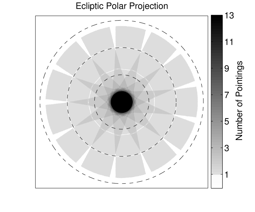
TESS will observe from a 13.7-day elliptical orbit around the Earth. Over two years, it will observe the sky using 26 pointings. Two spacecraft orbits (27.4 days) are devoted to each pointing. Because the cameras are fixed to the spacecraft, the spacecraft must re-orient for every pointing. The pointings are spaced equally in ecliptic longitude, and they are positioned such that the top camera is centered on the ecliptic pole and the bottom camera reaches down to an ecliptic latitude of 6∘. Figure 1 shows the hemispherical coverage resulting from this arrangement.
2.2. Spectral Response
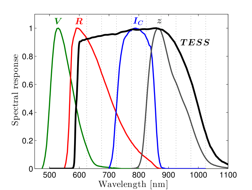
The spectral response of the TESS cameras is limited at its red end by the quantum efficiency of the CCDs. TESS employs the MIT Lincoln Laboratory CCID-80 detector, a back-illuminated CCD with a depletion depth of 100 m. This relatively deep depletion allows for sensitivity to wavelengths slightly longer than 1000 nm.
At its blue end, the spectral response is limited by a longpass filter with a cut-on wavelength of 600 nm. Figure 2 shows the the complete spectral response, defined as the product of the quantum efficiency and filter transmission curves.
| Spectral TypeaaThe mapping between and spectral type is based on data compiled by E. Mamajek. | photon fluxbbThe photon flux at is ph s-1 cm-2. | ||
|---|---|---|---|
| [K] | [ ph s-1 cm-2] | [mmag] | |
| M9V | 2450 | 2.38 | |
| M5V | 3000 | 1.43 | |
| M4V | 3200 | 1.40 | |
| M3V | 3400 | 1.38 | |
| M1V | 3700 | 1.39 | |
| K5V | 4100 | 1.41 | |
| K3V | 4500 | 1.43 | |
| K1V | 5000 | 1.45 | |
| G2V | 5777 | 1.45 | |
| F5V | 6500 | 1.48 | |
| F0V | 7200 | 1.48 | |
| A0V | 9700 | 1.56 |
It is convenient to define a TESS magnitude normalized such that Vega has . We calculate the photon flux by multiplying the template A0V spectrum provided by Pickles (1998) by the TESS spectral response curve and then integrating over wavelength. We assume Vega has a flux density of erg s-1 cm-2 Å-1 at Å (Hayes, 1985). We find that corresponds to a flux of erg s-1 cm-2, and a photon flux of ph s-1 cm-2.
By repeating the calculation for different template spectra from the Pickles (1998) library, we obtain the photon fluxes for stars of other spectral types. These are shown in Table 1. To facilitate comparisons with the standard Johnson-Cousins band (which is nearly centered within the -band), Table 1 also provides synthetic colors. We note that the color for an A0V star is , which is equal to the apparent magnitude defined for Vega.
2.3. Simplified model for the sensitivity of TESS
The most important stellar characteristics that affect planet detectability are apparent magnitude and stellar radius. Here we provide a simple calculation for the limiting apparent magnitude (as a function of stellar radius) that permits TESS to detect planets smaller than Neptune (). This gives an overview of TESS’s planet detection capabilities and establishes the necessary depth of our more detailed simulations of the population of nearby stars.
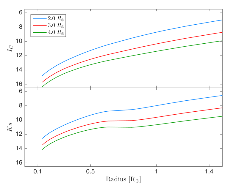
We assume the noise in the photometric observations to be the quadrature sum of read noise and the photon-counting noise from the target star and the zodiacal background (see Section 6.4 for the more comprehensive noise model). We require a signal-to-noise ratio of for detection (see Section 6.6 for the rationale). We assume that the total integration time during transits is 6 hours, which may represent two or more transits of shorter duration. Using these assumptions, Figure 3 shows the limiting apparent magnitude as a function of stellar radius at which transiting planets of various sizes can be detected.
To gauge the necessary depth of the detailed simulations, we consider the detection of small planets around two types of stars represented in Figure 3, a Sun-like star and an M dwarf with 3200 K. These two choices span the range of spectral types that TESS will prioritize; stars just larger than the Sun give transit depths that are too shallow, and dwarf stars just cooler than 3200 K are too faint in the TESS bandpass.
For the Sun-like star, a 4 planet produces a transit depth of 0.13%. The limiting magnitude for transits to be detectable is about . This also corresponds to and a maximum distance of 290 pc, assuming no extinction.
For the M dwarf with 3200 K, we assume , based on the Dartmouth Stellar Evolution Database (Dotter et al. 2008) for solar metallicity and an age of 1 Gyr. Since Dressing & Charbonneau (2015) found that M dwarfs very rarely have close-in planets larger than 3 , we consider a planet of this size rather than 4 . At 3 , the transit depth is 3.1% and the limiting apparent magnitude for detection is . This corresponds to and a maximum distance of 120 pc, assuming no extinction.”
A similar calculation can be carried out for eclipsing binary stars. Some TESS target stars will turn out to be eclipsing binaries, and others will be blended with faint binaries in the background. The maximum eclipse depth for an eclipsing binary is approximately 50%, which occurs when two identical stars undergo a total eclipse. Assuming the period is 1 day, and that TESS observes the system for 27.4 days, the limiting apparent magnitude for detection of the eclipse signals is , corresponding to many kiloparsecs.
To summarize, TESS is sensitive to small planets around Sun-like stars within 300 pc. For M dwarfs, the search distance is 100 pc.” Eclipsing binaries can be detected across the Milky Way. These considerations set the required depth of our simulations of the stellar population, which must also take into account the structure of the galaxy and extinction.
3. STAR CATALOG
Due to the wide range of apparent magnitudes that we need to consider, and the sensitivity of transit detections to stellar radii, we use a synthetic stellar population rather than a real catalog. The basis for our stellar population is TRILEGAL, an abbreviation for the TRIdimensional modeL of thE GALaxy (Girardi et al., 2005). TRILEGAL is a Monte Carlo population synthesis code that models the Milky Way with four components: a thin disk, a thick disk, a halo, and a bulge. Each of these components contains stars with the same initial mass function but with a different spatial distribution, star formation rate, and age-metallicity relation. For stars with masses 0.2-7 , TRILEGAL uses the Padova evolutionary tracks (Girardi et al., 2000) to determine the stellar radius, surface gravity, and luminosity as a function of age. For stars less massive than 0.2 , TRILEGAL uses a brown dwarf model (Chabrier et al., 2000). Apparent magnitudes in various photometric bands are computed using a spectral library drawing upon several theoretical and empirical sources. A disk extinction model is used to redden the apparent magnitudes depending on the location of the star. TRILEGAL does not include the Magellanic Clouds, nor does it model any star clusters.
The star counts predicted by the TRILEGAL model were originally calibrated against the Deep Multicolor Survey (DMS) and ESO Imaging Survey (EIS) of the South Galactic Pole. The model was also found to be consistent with the EIS coverage of the Chandra Deep Field South (Groenewegen et al., 2002). More recently, TRILEGAL was updated and re-calibrated against the shallower 2MASS and Hipparcos catalogs while maintaining agreement with the DMS and EIS catalogs (Girardi et al., 2005).
Given a specified line of sight and solid angle, TRILEGAL returns a magnitude-limited catalog of simulated stars, including properties such as mass, age, metallicity, surface gravity, distance, and extinction. Apparent magnitudes are reported in the Sloan , 2MASS , and Kepler bandpasses; at our request, L. Girardi kindly added the TESS bandpass to TRILEGAL. When necessary, we translate between the Sloan and Johnson-Cousins filters using the transformations for Population I stars provided by Jordi et al. (2006).
We find it necessary to adjust the properties of the population of low-mass stars () to bring them into satisfactory agreement with more recent determinations of the absolute radii and luminosity function of these stars. These modifications are described in Sections 3.2 and 3.4. In addition, we employ our own model for stellar multiplicity that is described in Section 3.3.
3.1. Model Queries
The TRILEGAL simulation is accessed through a web-based interface.111http://stev.oapd.inaf.it/cgi-bin/trilegal We use the default input parameters for the simulation (Table 2); the post facto adjustments that we make to dwarf properties, binarity, and the disk luminosity function are discussed below. The runtime of a TRILEGAL query is limited to 10 minutes, so we build an all-sky catalog by performing repeated queries over regions with small solid angles.
| Parameter | Value |
|---|---|
| Galactic radius of Sun | 8.70 kpc |
| Galactic height of Sun | 24.2 pc |
| IMF (log-normal, Chabrier 2001) | |
| Characteristic mass | 0.1 |
| Dispersion | 0.627 |
| Thin Disk | |
| Scale height (sech2) | 94.69 pc |
| Scale radius (exponential) | 2.913 kpc |
| Surface density at Sun | 55.4 pc-2 |
| Thick Disk | |
| Scale height (sech2) | 800 pc |
| Scale radius (exponential) | 2.394 kpc |
| Density at Sun | 10 pc-3 |
| Halo ( Oblate Spheriod) | |
| Major axis | 2.699 kpc |
| Oblateness | 0.583 |
| Density at Sun | 10 pc-3 |
| Bulge (Triaxial, Vanhollebeke et al. 2009) | |
| Scale length | 2.5 kpc |
| truncation length | 95 pc |
| Bar: aspect ratio | 0.68 |
| Bar-Sun angle | 15∘ |
| ratio | 0.31 |
| Central Density | 406 pc-3 |
| Disk Extinction | |
| Scale height (exponential) | 110 pc |
| Scale radius (exponential) | 100 kpc |
| Extinction at Sun () | 0.15 mag kpc-1 |
| 0.0378 mag | |
| Randomization (RMS) | 10 |
We divide the sky into 3072 equal-area tiles using the HEALPix scheme (Górski et al., 2005). Each tile subtends a solid angle of 13.4 deg2. For the 164 tiles closest to the galactic disk and bulge, the stellar surface density is too large for the necessary TRILEGAL computations to complete within the runtime limit. The high background level and high incidence of eclipsing binaries will also make these areas difficult to search for transiting planets, so we simply omit these tiles from consideration. This leaves 2908 tiles covering 95 of the sky.
For each of the 2908 sightlines through the centers of tiles, we make three queries to TRILEGAL:
-
1.
The “bright catalog” with and a solid angle of 6.7 deg. This is intended to include any star that could be searched for transiting planets; the magnitude limit of is based on the considerations in Section 2.3. Using the band to set the limiting magnitude is a convenient way to allow the catalog to have a fainter magnitude limit for M stars than for FGK stars. The full solid angle of 13.4 deg2 cannot be simulated due to the 10-minute maximum runtime of the simulation. Instead, we simulate a 6.7 deg2 field and simply duplicate each star in the catalog. Once duplicated, we assign coordinates to each star randomly from a probability distribution that is spatially uniform across the entire tile. Across all of the tiles, this catalog contains 1.58 stars.
-
2.
The “intermediate catalog” with and a solid angle of 0.134 deg2. This is intended to include stars for which TESS would be able to detect a deep eclipse of a binary star. We use this catalog to assign blended background binaries to the target stars in the bright catalog and also to evaluate background fluxes. This deeper query is limited to a smaller solid angle (1/100th of the area of the tile) to limit computational time. The simulation then re-samples from these stars 100 times when assigning background stars to the target stars. We also restrict this catalog to in the simulation to avoid double-counting stars from the bright catalog. Across all tiles, this catalog contains stars.
-
3.
The “faint catalog” with and a solid angle of 0.0134 deg2. This is used only to calculate background fluxes due to unresolved background stars. The limiting magnitude is not critical because the surface brightness due to unresolved stars is dominated by stars at the brighter end rather than the fainter end of the population of unresolved stars. Stars from this catalog are re-sampled 1000 times. Across all tiles, this catalog contains stars.
3.2. Properties of low-mass stars
Low-mass dwarf stars are of particular importance for TESS because they are abundant in the solar neighborhood and their small sizes facilitate the detection of small transiting planets. Although the TRILEGAL model is designed to provide simulated stellar populations with realistic distributions in spatial coordinates, mass, age, and metallicity, we noticed that the radii of low-mass stars for a given luminosity or in the TRILEGAL output were smaller than have been measured in recent observations or calculated in recent theoretical models.
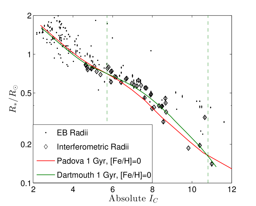
Figure 4 illustrates the discrepancy. It compares the radius-magnitude relation employed by TRILEGAL with that of the more recent Dartmouth models (Dotter et al., 2008) as well as empirical data based on optical interferometry of field stars and analysis of eclipsing binary stars. The interferometric radius measurements are from Boyajian et al. (2012). The measurements based on eclipsing binaries are from the compilation of Andersen (1991) that has since been maintained by J. Southworth222http://www.astro.keele.ac.uk/jkt/debcat/. We also include the systems tabulated by Winn et al. (2011b) in their study of Kepler-16. The published data specify rather than absolute magnitude; in preparing Figure 4, we converted into absolute using the temperature-magnitude data compiled by E. Mamajek333http://www.pas.rochester.edu/emamajek/EEM_dwarf_UBVIJHK_colors_Teff.txt and Pecaut & Mamajek (2013).
Figure 4 shows that the Dartmouth stellar-evolutionary models give better agreement with measured radii, especially those from interferometry. Therefore, to bring the key properties of the simulated stars into better agreement with the data, we replaced the TRILEGAL output for the apparent magnitudes and radii of low-mass stars (0.15-0.78 ) with the properties calculated with the Dartmouth models. To make these replacements, we use a trilateral interpolation in mass, age, and metallicity to determine the absolute magnitudes, , and radii from the grid of Dartmouth models. For simplicity, we assume the helium abundance is solar for all stars. Furthermore, motivated by Fuhrmann (1998), we only select the grid points that adhere to the following one-to-one relation between [/Fe] and [Fe/H]:
| (1) |
| (2) |
| (3) |
In calculating the apparent magnitudes of the stars with properties overwritten from the Dartmouth models, we preserve the distance modulus from TRILEGAL and apply reddening corrections using the same extinction model that TRILEGAL uses. TRILEGAL reports the extinction for each star, and for bands other than , we use the ratios from Cardelli et al. (1989).
3.3. Stellar Multiplicity
Binary companions to the TESS target stars have three important impacts on the detection of transiting planets. First, whenever a “target star” is really a binary, there are potentially two stars that can be searched for transiting planets. The effective size of the search sample is thereby increased. However, there is a second effect that decreases the effective size of the search sample: if there is a transit around one star, the constant light from the unresolved companion diminishes the observed transit depth, making it more difficult to detect the transit. Even if the transit is still detectable, the radius of the planet may be underestimated due to the diminished (or “diluted”) depth. The third effect is that a planet around one member of a close binary has a limited range of periods within which its orbit would be dynamically stable.
Furthermore, eclipsing binaries that are blended with target stars, or that are bound to the target star in hierarchical triple or quadruple systems, can produce eclipses that resemble planetary transits. Because eclipsing binaries produce larger signals than planetary transits, the population of eclipsing binaries needs to be simulated down to fainter apparent magnitudes than the target stars.
To capture these effects in our simulations, we need a realistic description of stellar multiplicity. We are guided by the review of Duchêne & Kraus (2013). The multiplicity fraction (MF) is defined as the fraction of systems that have more than one star; it is the sum of the binary fraction (BF), triple fraction (TF), quadruple fraction (QF), and so on. Our simulations consider systems with up to 4 stars.
The MF has been observed to increase with the mass of the primary, which is reflected in our simulation. In our TRILEGAL queries, every star is originally a binary, and we decide randomly whether to keep the secondary based on the primary mass and the MF values in Table 3. Next, we turn a fraction of the remaining binaries into triple and quadruple systems according to the desired TF and QF. The MF, TF, and QF are adopted as follows:
- 1.
- 2.
-
3.
For stars of mass 0.6-0.8 , we adopt an intermediate MF of 34%. The fraction of higher-order systems is .
-
4.
For primaries more massive than 1.4 , we use the results for A stars from Kouwenhoven et al. (2007), giving a MF of 75%. We assume that the fraction of higher-order systems is .
Next, we consider the properties of the binary systems. TRILEGAL originally creates binaries with a uniform distribution in the mass ratio between the secondary and the primary, , between 0.1 and 1. However, a more realistic distribution in is
| (4) |
where the power-law index is allowed to vary with the primary mass, as specified in Table 3. When we select the binary systems to obtain the desired MF, we choose the systems to re-create this distribution in over the range 0.11.0.
The period is not specified by TRILEGAL, so we assign it from a log-normal distribution. Duchêne & Kraus (2013) parametrizes the distribution in terms of the mean semimajor axis () and the standard deviation in ; both parameters vary with the primary mass as shown in Table 3. We convert from to with Kepler’s third law.
The orbital inclination is drawn randomly from a uniform distribution in . The orbital eccentricity is drawn randomly from a uniform distribution, between zero and a maximum value
| (5) |
where is specified in days, to provide a good fit to the range of eccentricities shown in Figure 14 of Raghavan et al. (2010). The argument of pericenter is drawn randomly from a uniform distribution between 0∘ and 360∘.
For the systems that are designated as triples, we assign the properties using the approach originally suggested by Eggleton (2009). Although there is no physical reason why this method should work well, it has been found to reproduce the multiplicity properties of a sample of Hipparcos stars (Eggleton & Tokovinin, 2008). First, we create a binary according to the prescriptions described above with a period . Then, we split the primary or secondary star (chosen randomly) into a new pair of stars. The new pair of stars orbit their barycenter with a higher-order period according to
| (6) |
where is uniformly distributed between 0 and 1. This procedure ensures that is the orbital period of the original binary system, a rudimentary method for enforcing dynamical stability. The mass of a star is conserved when it is split, so the barycenter of the original binary remains the same, and the orbital period of the companion star about this barycenter is unchanged.
The original prescription given by Eggleton (2009) assigns from a distribution peaking at days and allows the new period to vary over 5 decades. Since our assumed distribution for peaks at a shorter period (for stars 1 ), we only allow the higher-order orbital period to vary over 2 decades in our implementation. In this way, we avoid generating unphysically short periods.
The total mass of a new pair of stars is set equal to that of the original star, and the mass ratio is assigned in the following manner. The parent distribution of is taken from the sample of triples presented in Figure 16 of Raghavan et al. (2010). We model this distribution by setting for 23 of the pairs and drawing from a normal distribution with for the other 77% of the pairs. Finally, for each star in a higher-order pair, we calculate the absolute and apparent magnitudes, radius, and from the new stellar mass in combination with the age and metallicity inherited from the original star. We do so using the same interpolation onto the Dartmouth model grid described in Section 3.2.
For the systems that are turned into quadruples, we create a binary and then split both stars using the procedure described above. This results in two higher-order pairs that orbit one another with the original binary period .
| Mass [] | MF | [AU] | TF | QF | ||
|---|---|---|---|---|---|---|
| ¡0.1 | 0.22 | 4.5 | 0.5 | 4.0 | n/a | n/a |
| 0.1-0.6 | 0.26 | 5.3 | 1.3 | 0.4 | 0.067 | 0.017 |
| 0.6-0.8 | 0.34 | 20 | 2.0 | 0.35 | 0.089 | 0.023 |
| 0.8-1.0 | 0.41 | 45 | 2.3 | 0.3 | 0.11 | 0.030 |
| 1.0-1.4 | 0.50 | 45 | 2.3 | 0.3 | 0.14 | 0.037 |
| ¿1.4 | 0.75 | 350 | 3.0 | 0.20 | 0.055 |
3.4. Luminosity Function
| Primaries and Singles | Systems | Individual Stars | |
|---|---|---|---|
| 3.25 | 0.85 | 0.94 | 1.08 |
| 3.75 | 1.44 | 1.74 | 1.72 |
| 4.25 | 2.74 | 2.87 | 3.10 |
| 4.75 | 3.85 | 3.38 | 4.55 |
| 5.25 | 1.55 | 1.54 | 2.19 |
| 5.75 | 1.79 | 1.91 | 2.27 |
| 6.25 | 3.01 | 3.12 | 3.57 |
| 6.75 | 3.37 | 4.04 | 4.15 |
| 7.25 | 7.74 | 7.90 | 8.82 |
| 7.75 | 7.15 | 7.10 | 8.57 |
| 8.25 | 7.62 | 7.03 | 9.29 |
| 8.75 | 4.84 | 4.89 | 6.64 |
| 9.25 | 5.25 | 4.75 | 6.50 |
| 9.75 | 3.56 | 3.49 | 4.72 |
| 10.25 | 1.95 | 2.11 | 2.68 |
| 10.75 | 2.16 | 2.10 | 2.67 |
| 11.25 | 1.75 | 1.56 | 2.21 |
| 11.75 | 1.11 | 1.07 | 1.52 |
| 12.25 | 0.73 | 0.76 | 1.08 |
| 12.75 | 0.55 | 0.52 | 0.84 |
| 13.25 | 0.45 | 0.36 | 0.69 |
| 13.75 | 0.02 | 0.02 | 0.06 |
| 14.25 | 0.00 | 0.00 | 0.02 |
| 14.75 | 0.00 | 0.00 | 0.00 |
| 15.25 | 0.00 | 0.00 | 0.02 |
After modifying the TRILEGAL simulation to improve upon the properties of low-mass stars and assign multiple-star systems, we ensure that the luminosity function (LF) is in agreement with observations. For this purpose, we rely on two independent -band LFs reported in the literature. The first LF is from Cruz et al. (2007). It is based on volume-limited samples: a 20 pc sample for and an 8 pc sample for (Reid et al., 2003). Both samples use 2MASS photometry and are limited to . The second LF, from Bochanski et al. (2010), is based on data from the Sloan Digital Sky Survey for stars with . The resulting LF is reported for the range . Where the Cruz et al. (2007) and Bochanski et al. (2010) LFs overlap, we use the mean of the two LFs reported for single and primary stars (the brightest member of a multiple system). This results in the “empirical LF” to which the TRILEGAL LF is adjusted.
Next, we compute the LF of our TRILEGAL-based catalog by selecting all of the single and primary disk stars with distances within 30 pc. Then, we bin the stars according to and compare the result to the empirical LF. For each bin, we find the ratio of the TRILEGAL LF to the empirical LF. This ratio ranges from 0.5 to 11 across all of the magnitude bins.
We then return to each HEALPix tile individually, and we bin the stars by . Using the ratio computed above for each bin, we select stars at random for duplication or deletion to bring the simulated LF into agreement with the empirical LF. This process results in a net reduction of 30% in the total number of stars in the catalog and a shift in the LF peak towards brighter absolute magnitudes.
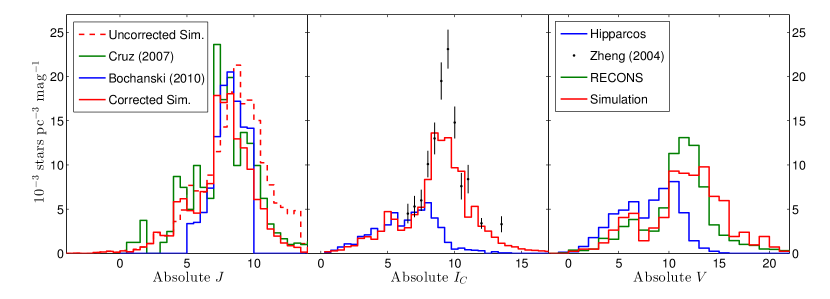
The left panel of Figure 5 shows the LF of the TRILEGAL simulation before and after this adjustment. The final LF is also quantified in Table 4. Each column of the table considers stellar multiplicity in a different fashion: “Singles and Primaries” counts single stars and the brightest member of a multiple system; “Systems” counts the combined flux of all stars in a system, regardless of whether it is single or multiple; and “Individual Stars” counts the primary and secondary members separately.
As a sanity check, we make some further comparisons between our simulated LF and other published luminosity functions. Figure 5 shows a comparison to the 10 pc RECONS sample (Henry et al., 2006), the Hipparcos catalog (Perryman et al. 1997 and van Leeuwen 2007), and the -band LF of Zheng et al. (2004). The agreement with the Hipparcos sample is good up until , where the Hipparcos sample becomes incomplete. The RECONS LF has a lower and blunter peak, and the Zheng et al. (2004) LF has a sharper and taller peak than the simulated LF, but are otherwise in reasonable agreement.
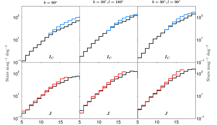
As another sanity check, we examine star counts as a function of limiting apparent magnitude in Figure 6. We compare the number of stars per unit magnitude per square degree in the simulated stellar population against star counts from the classic Bahcall & Soneira (1981) star-count model in the band as well as actual star counts from the 2MASS point source catalog (Skrutskie et al., 2006) in the band. In all cases, multiple systems are counted as a single “star” with a magnitude equal to the total system magnitude. The agreement seems satisfactory; we note that the comparison with 2MASS becomes less reliable at faint magnitudes because of photometric uncertainties as well as extra-galactic objects in the 2MASS catalog.
3.5. Stellar Variability
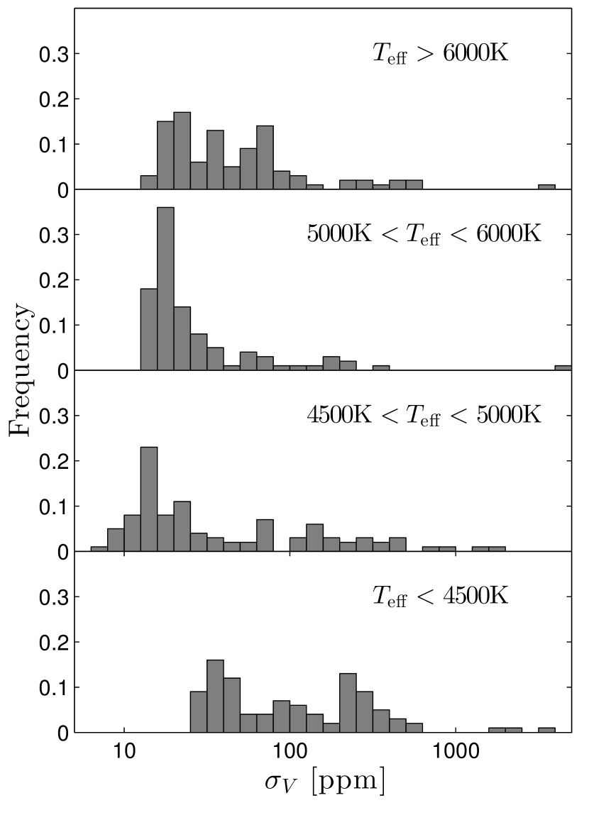
Intrinsic stellar variability is a potentially significant source of photometric noise for the brightest stars that TESS observes. To each star in the simulation, we assign a level of intrinsic photometric variability from a distribution corresponding to the spectral type. Our assignments are based on the variability of Kepler stars reported by Basri et al. (2013). For each star, they calculated the median differential variability (MDV) on a 3-hour timescale by binning the light curve into 3-hour segments and then calculating the median of the absolute differences between adjacent bins. Since each transit is a flux decrement between one segment of a light curve relative to a much longer timeseries, rather than two adjacent segments of equal length, the noise statistic relevant to transit detection is approximately smaller than the MDV.
G. Basri kindly provided the data from their Figures 7-10. Their sample is divided into four subsamples according to stellar . We select 100 stars in each subsample with to minimize the contributions of instrumental noise from Kepler. Since red giants exhibiting pulsations can contaminate the subsample with K, particularly at brighter apparent magnitudes, we select stars with for these temperatures.
Figure 7 shows the resulting distributions of variability. Each star in our simulated population is assigned a variability index from a randomly-chosen member of the 100 stars in the appropriate subsample. The variability of the K subsample is roughly 5 times greater than that of solar-type stars. However, M dwarfs are the faintest stars that TESS will observe, so instrumental noise and background will dominate the photometric error of these targets.
Since the photometric variations associated with stellar variability exhibit strong correlations on short timescales, we assume that the level of noise due to intrinsic variability is independent of transit duration: we do not adjust it according to as would be the case for white noise. However, we do assume that stellar variations are independent from one transit to the next, so the noise contribution from stellar variability scales with the number of transits as . In summary, the standard deviation in the relative flux due to stellar variability, after phase-folding all of the transits together, is taken to be
| (7) |
4. ECLIPSING SYSTEMS
We next assign planets to the simulated stars, and we identify the transiting planets as well as the eclipsing binaries. We then calculate the properties of the transits and eclipses relevant to their detection and follow-up.
4.1. Planets
The planet assignments are based on several recent studies of Kepler data. The Kepler sample has high completeness for the planetary periods ( days) and radii () that are most relevant to TESS.
For FGK stars, we adopt the planet occurrence rates from Fressin et al. (2013). For K, we adopt the occurrence rates from Dressing & Charbonneau (2015), who updated the results that were originally presented by Dressing & Charbonneau (2013). We note that Dressing & Charbonneau (2015) corrected their planet occurrence rates for astrophysical false positives by using the false-positive rates presented by Fressin et al. (2013) as a function of the apparent planet size.
In both cases, the published results are provided as a matrix of occurrence rates and uncertainties for bins of planetary radius and period. The incompleteness of the Kepler sample is considered for each bin. Because the bins are relatively coarse, we allow the radius and period of a given planet to vary randomly within the limits of each bin. Periods are assigned from a uniform distribution in . (We omit planets for which the selected period would place the orbital distance within , on the grounds that tidal forces would destroy any such planets.)
For the smallest radius bin examined by Fressin et al. (2013), we choose the planet radius from a uniform distribution between 0.8–1.25 . For the larger-radius bins, we choose the planet radius within each bin according to the distribution
| (8) |
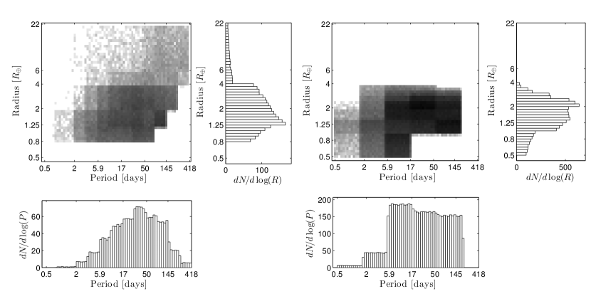
These intra-bin distributions were chosen ad hoc to provide a relatively smooth function in the radius–period plane. Likewise, when applying the occurrence rates from Dressing & Charbonneau (2015), for the smallest radius bin we choose the planet radius from a uniform distribution between 0.5–1.0 . For the bin extending from 1.0–1.5) , we chose the planet radius from a distribution with a power-law index of . For we use a power-law index of . The maximum planet size in the Fressin et al. (2013) matrix is 22 , and the maximum planet size in the Dressing & Charbonneau (2015) matrix is 4 . The final distributions are illustrated in Figure 8.
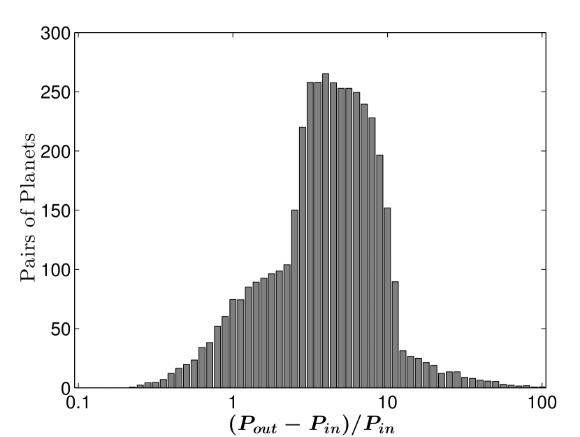
We allow our simulation to assign more than one planet to a given star with independent probability. The only exceptions are (1) we require the periods of adjacent planetary orbits to have ratios of at least 1.2, and (2) planets around a star with a binary companion cannot have orbital periods that are within a factor of 5 of the binary orbital period. The result is that 53 of the transiting systems around FGK stars and 55 of those around M stars are multiple-planet systems. Figure 9 shows the resulting distribution of period ratios. The orbits of multi-planet systems are assumed to be perfectly coplanar, both for simplicity and from the evidence for low mutual inclinations in compact multi-planet systems (Fabrycky et al., 2014; Figueira et al., 2012).
As a sanity check, we compare the proportion of planets in multi-transiting systems in our simulated stellar population to the proportion of multi-transiting Kepler candidates. In our simulation, 26.2 of planets around FGK stars and 33.6 of planets around M stars reside in multi-transiting systems. Out of the 4,178 Kepler objects of interest, 41 are in multi-transiting systems.
For simplicity, we assume that all planetary orbits are circular. The orbital inclinations are assigned randomly from a uniform distribution in . We identify the transiting systems as those with , where
| (9) |
is the transit impact parameter.
We then calculate the properties of the planets and their transits and occultations. The transit duration is given by Eqns. (18) and (19) of Winn (2011) in terms of the mean stellar density :
| (10) |
The depth of the transit is given by . The depth of the occultation (secondary eclipse) is found by estimating the effective temperature of the planet () and then computing the photon flux within the TESS bandpass from a blackbody of radius . The photon flux from the planet is then divided by the combined photon flux from the planet and the star:
| (11) |
The equilibrium planetary temperature is determined by assuming radiative equilibrium with an albedo of zero and isotropic radiation (from a recirculating atmosphere), giving
| (12) |
We also keep track of the relative insolation of the planet , defined as
| (13) |
4.2. Eclipsing Binaries
We identify the eclipsing binaries by computing the impact parameters and of the primary and secondary eclipses, respectively:
| (14) |
(see Eqns. 7-8 of Winn 2011). Non-grazing primary eclipses are identified with the criterion
| (15) |
while grazing primary eclipses have larger impact parameters:
| (16) |
The eclipse depth of non-grazing primary eclipses is given by
| (17) |
where and are the photon fluxes from each star. In the event that , the area ratio is set equal to unity; in that case, the primary undergoes a total eclipse. We neglect limb-darkening in these calculations for simplicity. Secondary eclipses are identified and quantified in a similar manner.
For grazing eclipses, the area ratio is replaced with the overlap area of two uniform disks with the appropriate separation of their centers, given by Eqns. (2.14-5) of Kopal (1979). The durations and timing of eclipses are calculated from Eqns. (14-16) of Winn (2011).
We discard eclipsing binaries when the assigned parameters imply or . We also exclude systems where is less than the Roche limit for either star, assuming they are tidally locked:
| (18) |
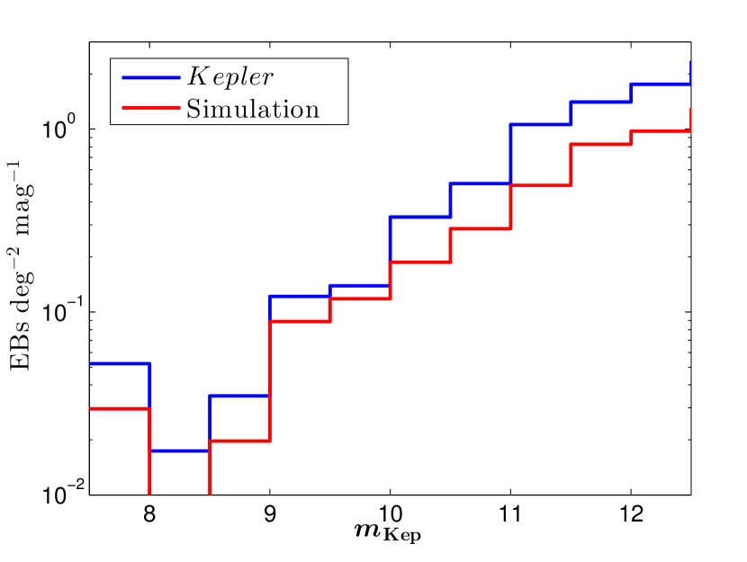
For primaries with , our simulated stellar population has 97461 eclipsing binaries over the of the sky that is covered by the simulation. Another 21441 systems contain eclipsing pairs in a hierarchical system. As another sanity check, we compare the simulated density of eclipsing systems on the sky to the catalog of eclipsing binaries in the Kepler field. We use Version 2 of the compilation444http://keplerebs.villanova.edu/v2 from Prša et al. (2011) and Slawson et al. (2011) to plot the density of eclipsing binaries as a function of apparent system magnitude in Figure 10. Within the range of days, this catalog contains 1.85 EBs deg-2 with . A 203 deg2 subsample of our TRILEGAL catalog, taken from 15 HEALPix tiles and centered on galactic coordinates and for similarity to the Kepler field, contains 1.04 EBs deg-2 with . This disparity suggests that our model of the eclipsing-binary population could have systematic errors of nearly 80%, at least for the relatively low galactic latitude of the Kepler field, where the TRILEGAL simulation loses accuracy, and the steep increase in the stellar surface density makes it difficult to accurately match the simulation results to the Kepler field.
5. BEST STARS FOR TRANSIT DETECTION
Now that planets have been assigned to all of the stars with , it is interesting to explore the population of nearby transiting planets independently from how they might be detected by TESS or other surveys. This helps to set expectations for the brightest systems that can reasonably be expected to exist with any desired set of characteristics.
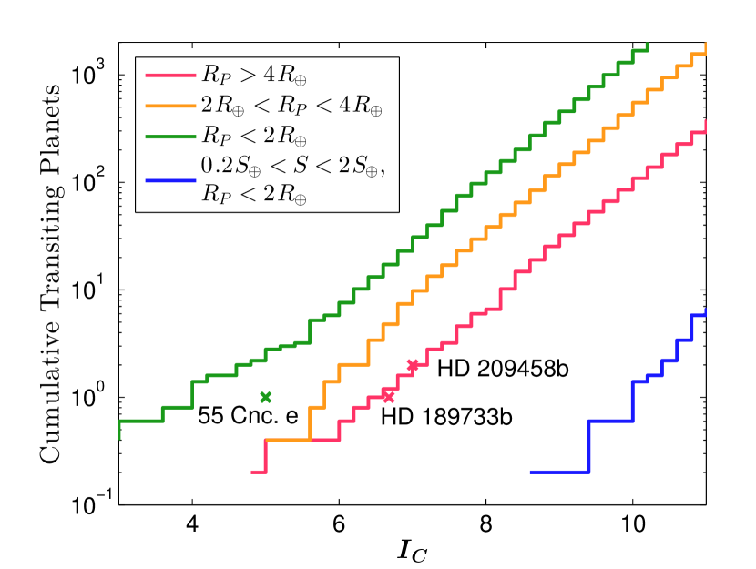
First, we identify the brightest stars with transiting planets. Figure 11 shows the cumulative number of transiting planets as a function of the limiting apparent magnitude of the host star. This is equal to the total number of planets that would be detected in a 95% complete magnitude-limited survey (since our HEALPix tiles cover this fraction of the sky). We include the stars with effective temperatures between 2000 and 7000 K and that host planets with periods 20 days. To reduce the statistical error, we combine the outcomes of 5 trials.
The brightest star with a transiting planet of size 0.8-2 has an apparent magnitude . The tenth brightest such star has . For transiting planets of size 2-4 , the brightest host star has and tenth brightest has . One must look deeper in order to find potentially habitable planets with periods shorter than 20 days; if we require and , the brightest host star has and the tenth brightest has . (While there is also an outer limit to the HZ, we do not impose a lower limit on since transit surveys are biased toward close-in planets.)
In reality, the brightest host stars could be brighter or fainter than the expected magnitudes. In Figure 11 we also show the brightest known transiting systems for some of the categories. Their agreement with the simulated cumulative distributions suggest that some of the very brightest transiting systems have already been discovered.
6. INSTRUMENT MODEL
Now that the simulated population of transiting planets and eclipsing binaries has been generated, the next step is to calculate the signal-to-noise ratio (SNR) of the transits and eclipses when they are observed by TESS. The signal is the fractional loss of light during a transit or an eclipse (), and the noise () is calculated over the duration of each event. The noise is the quadrature sum of all the foreseeable instrumental and astrophysical components.
Evaluation of the SNR is partly based on the parameters of the cameras already described in Section 2. We also need to describe how well the TESS cameras can concentrate the light from a star into a small number of pixels. The same description will be used to evaluate the contribution of light from neighboring stars that is also collected in the photometric aperture.
Our approach is to create small synthetic images of each transiting or eclipsing star, as described below. These images are then used to determine the optimal photometric aperture and the SNR of the photometric variations.
The synthetic images are also used to study the problem of background eclipsing binaries. Transit-like events that are apparent in the total signal measured from the photometric aperture could be due to the eclipse of any star within the aperture. With only the photometric signal, there is no way to determine which star is eclipsing. If the timeseries of the and coordinates of the flux-weighted center of light (the “centroid”) is also examined, then in some cases, one can determine which star is undergoing eclipses. As shown in Section 8.4, background eclipsing binaries tend to produce larger centroid shifts during eclipses than transiting planets. The synthetic images allow us to calculate the centroid during and outside of transits and eclipses.
6.1. Pixel response function
The synthetic images are constructed from the pixel response function (PRF), which describes the fraction of light from a star that is collected by a given pixel. It is calculated by numerically integrating the point-spread function (PSF) over the boundaries of pixels. The photometric aperture for a star is the collection of pixels over which the electron counts are summed to create the photometric signal; they are selected to maximize the photometric SNR of the target star. Throughout this study, we assume that the pixel values are simply summed without any weighting factors.
The TESS lens uses seven elements with two aspheres to deliver a tight PSF over a large focal plane and over a wide bandpass. Due to off-axis and chromatic aberrations, the TESS PSF must be described as a function of field angle and wavelength. We calculate the PSF at four field angles from the center (0∘) to the corner (17∘) of the field of view. Chromatic aberrations arise both from the refractive elements of the TESS camera and from the deep-depletion CCDs absorbing redder photons deeper in the silicon. We calculate the PSF for nine wavelengths, evenly spaced by 50 nm, between 625 and 1025 nm. These wavelengths are shown with dashed lines in Figure 2. These wavelengths also correspond to a set of bandpass filters that will be used in the laboratory to measure the performance of each flight TESS camera.
The TESS lens has been modeled with the Zemax ray-tracing software. We use the Zemax model to trace 250,000 simulated rays through the camera optics for each field angle and wavelength. The model is set to the predicted operating temperature of C. Rays are propagated through the optics and then into the silicon of the CCD. A probabilistic model is used to determine the depth of travel in the silicon before the photons are converted to electrons. Finally, the diffusion of the electrons within the remaining depth of silicon is modeled to arrive at the PSF.
Pointing errors from the spacecraft will effectively enlarge the PSF because the 2 sec exposures are summed into 2 min stacks without compensating for these errors. The spacecraft manufacturer (Orbital Sciences) has provided a simulated time series of spacecraft pointing errors from a model of the spacecraft attitude control system. Using two minutes of this time series, we offset the PSF according to the pointing error and then stack the resulting time series of PSFs. The root-mean-squared (rms) amplitude of the pointing error is , which is small in comparison to the pixel size and the full width half-maximum of the PSF. Thus, the impact of pointing errors on short timescales turns out to be minor. Long-term drifts in the pointing of the cameras will also introduce photometric errors, but this effect is budgeted in the systematic error described in Section 6.4.2.
Limits in the manufacturing precision of TESS cameras will also increase the size of the PSF from its ideal value. In a Monte Carlo simulation drawing from the tolerances prescribed in the optical design, the the fraction of the flux captured by the brightest pixel in the PRF is reduced by in 80 of cases. To capture this effect, we simply increase the size of the PSF by to achieve the same reduction.
Even after considering jitter and manufacturing errors, the PSF is still under-sampled by the 15 m pixels of the TESS CCDs. Therefore, we must recalculate the PRF for a given offset and orientation between the PSF and the pixel boundaries. We numerically integrate the PSF over a grid of pixels to arrive at the PRF. We do so over a grid of sub-pixel centroid offsets and two different azimuthal orientations (0∘ and 45∘) with respect to the pixel boundaries. For the corner PSF (at a field angle of 17∘), only the 45∘ azimuth angle is considered.
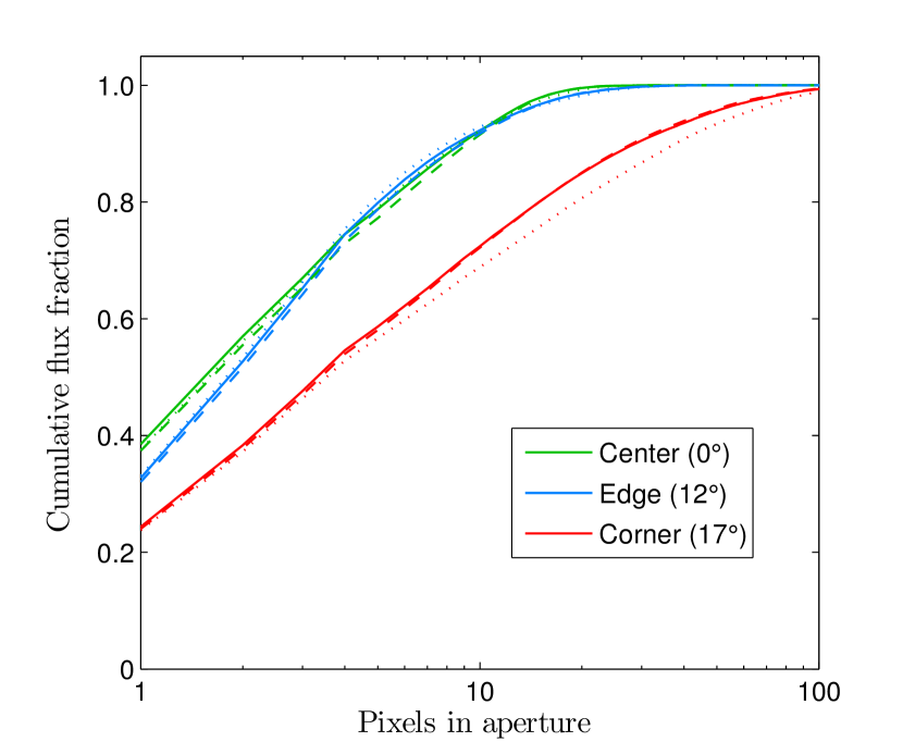
We can also view the PRF in terms of the cumulative fraction of light collected by a given number of pixels. In Figure 13, we average over all of the centroid offsets and both azimuthal angles. For clarity, only three of the field angles and three values of are shown. There is little change in the PRF across the range of , but the PRF degrades significantly at the corners of the field.
6.2. Synthetic images
For each target star with eclipses or transits, we create a synthetic image in the following manner. First, we determine the appropriate PRF based on the star’s color and location in the camera field. We calculate the field angle from its ecliptic coordinates and the direction in which the relevant TESS camera is pointed. We randomly assign an offset between the star and the nearest pixel center, and we randomly assign an azimuthal orientation of either 0∘ or 45∘. We then look up the nine wavelength-dependent PRFs for the appropriate field angle, centroid offset, and azimuthal angle. The nine PRFs are summed with weights according to the stellar effective temperature.
The weight of a given PRF is proportional to the stellar photon flux integrated over the wavelengths that the PRF represents. Outside of the main simulation, we considered a Vega-normalized stellar template spectrum of each spectral type from the Pickles (1998) library. We multiplied each template spectrum by the spectral response function of the TESS camera, and we integrated the photon flux for each of the nine PRF bandpasses. Next, we fitted a polynomial function to the relationship between the stellar effective temperatures and the photon flux in each bandpass. During the simulation, the polynomial functions are used to quickly calculate the appropriate PRF weights as a function of stellar effective temperature.
Once the PRFs are summed, the result is a synthetic -pixel image of each target star. We only consider the central pixels when determining the optimal photometric aperture; the left panel of Figure 12 shows an example.

After synthesizing the image of each eclipsing or transiting target star, a separate image is synthesized of all the relevant neighboring stars and companion stars. The neighboring stars are drawn from all three star catalogs described in Section 3. The stars are assumed to be uniformly distributed across each HEALPix tile, allowing us to randomly generate the distances between the target star and the neighboring stars. Stars from the target catalog are added to the synthesized image if they are within a radius of 6 pixels from the target star. Stars from the intermediate catalog are added if they are within 4 pixels, and stars from the faint catalog are added if they are within 2 pixels. The synthesized images are created in the same manner as described above: by weighting, shifting, and summing the PRFs associated with each star. The right panel of Figure 12 shows an example.
Synthetic images are also created for the eclipsing binary systems drawn from the intermediate catalog, but a slightly different approach is taken. For each eclipsing binary, we search for any target stars within 6 pixels. If any are found, the brightest is added to the list of target stars with apparent transits or eclipses. Separate synthetic images are created for the target star, the eclipsing binary, and the non-eclipsing neighboring stars. Hierarchical binaries are treated in a similar fashion; the non-eclipsing component is treated as the target star, and a separate synthetic image is created for the eclipsing pair so that its apparent depth can be diluted. While this approach may appear to strongly depend upon the somewhat arbitrary magnitude limits adopted for the different catalogs, this is not really the case. Both the eclipsing binaries from the target catalog and the background eclipsing binaries from the intermediate catalog end up being diluted by neighboring stars drawn from all of the catalogs.
6.3. Determination of optimal aperture
For each target star that is associated with an eclipse or transit (whether it is due to the target star itself or a blended eclipsing binary), we select the pixels that provide the optimal photometric aperture from the central pixels of its synthetic image. Starting with the three brightest pixels in the PRF, we add pixels in order decreasing brightness one at a time. At each step, we sum the flux of the pixels from the synthetic image of target star and from the synthetic image of the neighboring stars. We also consider the read noise and zodiacal noise, which are discussed in Section 6.4. As the number of pixels in the photometric aperture increases, more photons are collected from the target star, and more noise is accumulated from the readout, sky background, and neighboring stars. The optimal photometric aperture maximizes the SNR of the target star even if the eclipse is produced by a blended binary. We assume that the data will be analyzed with prior knowledge of the locations of neighboring stars (but no prior knowledge of whether they eclipse).
Once the optimal aperture is determined, we calculate the dilution parameter , which is the factor by which the true eclipse or transit depth is reduced by blending with other stars in the photometric aperture. Specifically, the dilution parameter is defined as the ratio of the total flux in the aperture from the neighboring stars () and target star () to the flux from the target star:
| (19) |
For blended binaries and hierarchical systems, the denominator is replaced with the flux from the binary , and the target star becomes a source of dilution:
| (20) |
With this definition, signifies an isolated system, and in general, . This parameter is later reported for all detected eclipses under the “Dil.” column of Table 6.
6.4. Noise Model
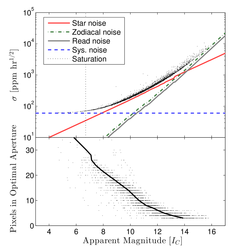
The photometric noise model includes the photon-counting noise from all of the stars in the photometric aperture, photon-counting noise from zodiacal light, stellar variability, and instrumental noise. Stellar variability and background stars are randomly assigned from distributions, while the other noise terms are more deterministic in nature. Figure 14 shows the relative photometric noise as a function of apparent magnitude and also breaks down the contributions from the deterministic sources of noise. Each subsection below describes the noise terms in more detail.
6.4.1 Zodiacal Light
Although TESS avoids the telluric sky background by observing from space, it its still affected by the zodiacal light (ZL) and its associated photon-counting noise. Our model of the zodiacal flux is based on the spectrum measured by the Space Telescope Imaging Spectrograph on the Hubble Space Telescope.555http://www.stsci.edu/hst/stis/performance/background/skybg.html We multiply this ZL spectrum by the TESS spectral response function and integrate over wavelength. This gives the photon flux of
| (21) |
where is the -band surface brightness of the ZL in mag arcsec-2. For TESS, the pixel scale is and the effective collecting area is 69 cm2. To model the spatial dependence of , we fit the tabulated values of as a function of helio-ecliptic coordinates666http://www.stsci.edu/hst/stis/documents/handbooks/currentIHB/c06_exptime6.html#689570 with a function
| (22) |
where is the ecliptic latitude and and are free parameters. Because TESS will generally be pointed in the anti-solar direction (near helio-ecliptic longitude ), and because depends more strongly on latitude than longitude in that region, we only fitted to the data with and weighted the points in proportion to . The least-squares best-fit has mag and mag.
Based on these results, we find that the zodiacal light collected in a 2 sec image ranges from 95-270 pix-1 depending on ecliptic latitude. The photon-counting noise associated with this signal varies from 10-16 pix-1 RMS, as mentioned in Section 2.
6.4.2 Instrumental Noise
The read noise of the CCDs is assumed to be 10 pix-1 RMS in each 2 sec exposure, which is near or below the level of photon-counting noise from the ZL. Both the read noise and ZL noise grow in proportion to the square root of the number of pixels used in the photometric aperture.
Our noise model for TESS cameras also includes a systematic error term of 60 ppm hr1/2. This is an engineering requirement on the design rather than an estimate of a particular known source of error. We assume that the systematic error is uncorrelated and scales with the total observing time as . Under these assumptions, the systematic error grows larger than 60 ppm for timescales shorter than one hour, which is probably unrealistic; however, this issue is not very relevant to our calculations because such timescales are shorter than the typical durations of transits and eclipses.
It is thought that the systematic error of the TESS cameras will primarily stem from pointing errors that couple to the photometry through non-uniformity in the pixel response. These pointing errors come from the attitude control system, velocity aberration, thermal effects, and mechanical flexure. In addition, long-term drifts in the camera electronics can contribute to the systematic error. The data reduction pipeline will use the same co-trending techniques that were used by the Kepler mission to mitigate these effects, but the exact level of residual error that TESS will be able to achieve is unknown at this time.
6.4.3 Saturation
Stars with will saturate the innermost pixels of the PRF during the 2-second exposures. For reference, this saturation magnitude is identified with a dotted line in Figure 14. These saturated stars represent of the target stars. As was the case with the Kepler CCDs, the TESS CCDs are designed to conserve the charge that bleeds from saturated pixels, and do not use anti-blooming structures. Since photometry of saturated stars with Kepler has achieved the photon-counting limit (Gilliland et al., 2011), we assume that the systematic error is the same for the saturated stars and the unsaturated stars.
While large photometric apertures will be needed to collect all of the charge that bleeds from saturated stars, the read and zodiacal noise are not important since the photometric precision will be dominated by photon-counting noise and systematic errors. Because the photometric precision will not depend strongly upon the number of pixels used in the photometric aperture, we do not model the saturated stars differently in our simulation.
6.4.4 Cosmic Rays
Typical back-illuminated CCDs have depletion depths of 10-50 m. In contrast, the TESS CCDs have a 100 m depletion depth. This is desirable to enhance the quantum efficiency at long wavelengths, but it also makes the detectors more susceptible to cosmic rays (CRs) since the pixel volume is larger and the maximum amount of charge collected per event can be larger.
To assess the effect of cosmic rays, we consider a typical cosmic ray flux of 5 events s-1 cm-2 and minimally-ionizing events that deposit 100 m-1 within silicon. Each pixel has an optical exposure time of 2 sec. The accumulated images also spend an average of 1 sec in the frame-store region of the CCD, where they are still vulnerable to cosmic rays. Given these parameters, for each 2 min stack of values from one pixel, there is a 10% chance of experiencing a cosmic ray event with an energy deposition above the combined read and zodiacal noise of 110 . The distribution in the energy deposition values has a peak near 1500 , which is comparable to the photon-counting noise of bright stars observed with 2 min cadence. Electrons from cosmic rays will therefore add significantly to the photometric noise, but will not be easily detected in the 2 min or 30 min data products.
Cosmic rays are far more conspicuous in the 2 sec images. Therefore, it is probably best to remove the contaminated pixel values before they are combined into the 2 min and 30 min stacks. The Data Handling Unit on TESS will apply a digital filter that rejects outlier values during the stacking process either periodically or adaptively. A possible side-effect of this filter, depending on the algorithm used, is a reduction in the signal-to-noise ratio to the degree that uncontaminated data is also rejected in the absence of cosmic rays.
The exact algorithm that will be used to mitigate cosmic-ray noise is still being studied. For the present simulations we have budgeted for a 3 loss in the SNR. In the simulation code, we simply raise the detection threshold (described in Section 6.6) by 3 to compensate for the reduced SNR, and we assume that there are no other residual effects from cosmic rays.
6.5. Duration of observations
The SNR of transits or eclipses will depend critically on how long the star is observed. Figure 1 is a sky map showing the number of times that TESS will point at a given location as a function of ecliptic coordinates. As noted above, the simulations assign coordinates to each star through a uniform random distribution across the HEALPix tile to which it belongs. The star’s ecliptic coordinates are then converted to and pixel coordinates for each TESS pointing. We tally the number of pointings for which the target falls within the field-of-view of a TESS camera. The total amount of observing time is calculated as the total duration of all consecutive pointings.
The duty cycle of observations must also be considered. At each orbital perigee, TESS interrupts observations in order to transmit data to Earth and perform other housekeeping operations. This takes approximately 0.6 days. We model this interruption in the simulation, so each 13.6-day spacecraft orbit actually results in 13.0 days of data.
The presence of the Earth or Moon in the field-of-view of any camera will also prohibit observations. We do not model this effect since predicting their presence depends upon the specific launch date of TESS. However, our simulations do show that if observations are interrupted near TESS’s orbital apogee in addition to its perigee, then the planet yields are approximately proportional to the duty cycle of observations.
6.6. Detection
The model for the detection process is highly simplified: we adopt a threshold for the signal-to-noise ratio, and we declare a signal to be detected if the total SNR exceeds the threshold. In other words, the detection probability is modeled as a step function of the computed SNR. (The matched-filter technqiues of the TESS pipeline probably have a smoother profile, such as a standard error function [Jenkins et al. 1996]). For transiting planets, all of the observed transits contribute to the total SNR. For eclipsing binaries, we allow both the primary and secondary eclipses to contribute to the total SNR.
The choice of an appropriate SNR threshold was discussed in detail by Jenkins et al. (2002) in the context of the Kepler mission. Their criterion was that the threshold should be sufficiently high to prevent more than one “detection” from being a purely statistical fluke after analyzing all of the data from the entire mission. We adopt the same criterion here. Since the number of astrophysical false positives is at least several hundred (as discussed below), this criterion allows statistical false positives to be essentially ignored.
To determine the appropriate threshold, we use a separate Monte Carlo simulation of the transit search. We produce light curves containing uncorrelated, Gaussian noise and analyze them for transits in a similar manner as will be done with real data. Then, we find the SNR threshold that results in approximately one statistical false positive. Each light curve consists of 38,880 points, representing two 27.4-day TESS pointings with 2-minute sampling. We chose a timeseries length of two pointings rather than one to account for the stars observed with overlapping pointings.
To search for transits, we scan through a grid of trial periods, times of transit, and transit durations. At each grid point, we identify the data points belonging to the candidate transit intervals. The SNR is computed as the mean of the in-transit data values divided by the uncertainty in the mean.
The grid of transit durations starts with 28 min (14 samples) and each successive grid point is longer by 4 min (2 samples). The grid of periods is the range of periods that are compatible with the transit duration. The periods are calculated by inverting Eqn. (10):
| (23) |
We allow to vary over a sufficient range to include plausible stellar densities from 0.5 to 100. The fractional step size in the period is then , which has a minimum value of 0.43 for the shortest periods. We consider orbital periods ranging from 1.7 hr (which is below the period corresponding to Roche limit) to 27.4 days (half of the nominal observing interval). The transit phase is stepped from zero to the orbital period in increments of one-half the transit duration.
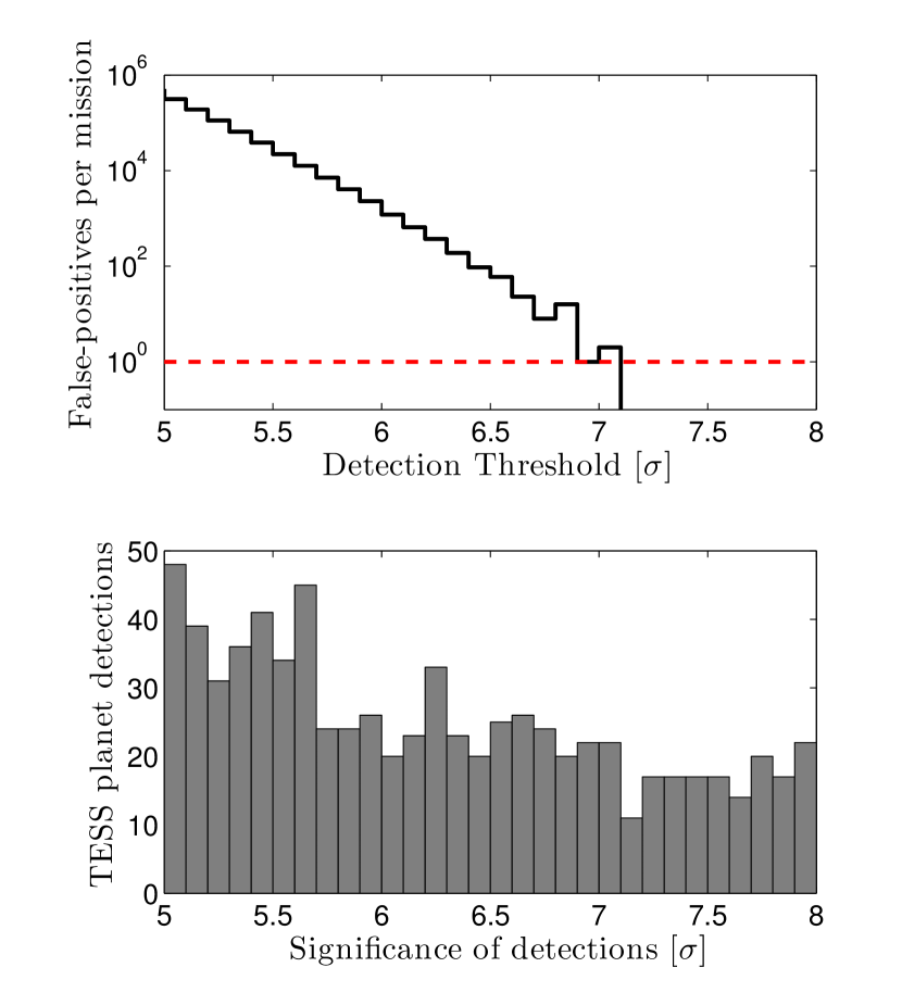
Figure 15 shows how the number of false-positive detections scales with the detection threshold. We find that a SNR of 7.1 produces approximately one statistical false positive within the library of light curves. By coincidence, this is equal to the SNR threshold of 7.1 that was calculated for Kepler mission by Jenkins et al. (2002). TESS searches twice as many stars as the considered in the Kepler study, and over a larger dynamic range in period; Kepler searches for planets with longer periods using longer intervals of data.
To account for the expected reduction in SNR due to the cosmic-ray rejection algorithm (see Section 6.4.4), we adopt a slightly higher threshold of 7.3 in this paper. In addition, we only consider a transit or eclipse to be detected if two or more events are observed. We also record the single events that exceed the SNR threshold, but we do not count them as “detections” in the tallies and the discussion that follows. The planets detected with a single transit generally have longer periods than the multiple-transit detections. It is also worth noting that TESS may detect some single transits from the population of planets with periods longer than a year, which we have not simulated at all, because our sources for planet occurrence rates do not extend to such long periods. The single-transit detections may represent interesting opportunities to study the properties of more distant planets. However, they will require additional ground-based follow-up observations to determine the orbital period and discriminate against astrophysical or statistical false positives.
6.7. Selection of target stars
From the 1.58 stars in the catalog, we must select the target stars for which pixel data will be saved and transmitted with 2 min time sampling. In our simulation, the target stars are chosen according to the prospects for detecting the transits of small planets, which depend chiefly on stellar radius and apparent magnitude.
In the simulation, we have complete knowledge of the properties of each star, which makes it straightforward to determine whether a fiducial transiting planet with a given radius and period could be detected with TESS. We adopt an orbital period of 20 days; for each 27.4-day pointing that TESS spends observing a star, we assume that 2 transits are observed. The stellar radius and mass are used to calculate the transit duration with a 20-day period, thereby determining the total exposure time during transits. Then, we use the simplified noise model from Section 2.3 that considers the read noise and photon-counting noise of the star and zodiacal light. We then check to see if the fiducial transiting planet would be detectable with a signal-to-noise ratio exceeding of 7.3.
The number of stars meeting this detection criterion depends strongly on the radius of the fiducial planet. Starting from small values, we increase the radius until the number of stars for which the planet would be detectable is . This is achieved for . Through this procedure, the target star catalog is approximately complete for planets smaller than 2.25 with orbital periods shorter than 20 days. There is a higher density of target stars assigned near the ecliptic poles due to the longer duration of TESS observations in those regions.
In selecting the target stars, we do not assume prior knowledge of whether a star is part of a multiple-star system. If it is, we assume that all components of the system fall within a single photometric aperture, and they are all observed at the 2 min cadence.
Figure 16 illustrates the selection of the target stars on a Hertzsprung-Russell diagram. For clarity, we show a magnitude-limited subsample () of our “bright” catalog as well as a randomly-selected subsample of the target stars. Nearly all main-sequence stars with K are selected as target stars. Stars that are larger than the Sun are only included if they have a sufficiently bright apparent magnitude. White dwarfs could also be interesting targets for TESS, but we do not include them in our simulation because the occurrence rates of planets around white dwarfs is unknown.
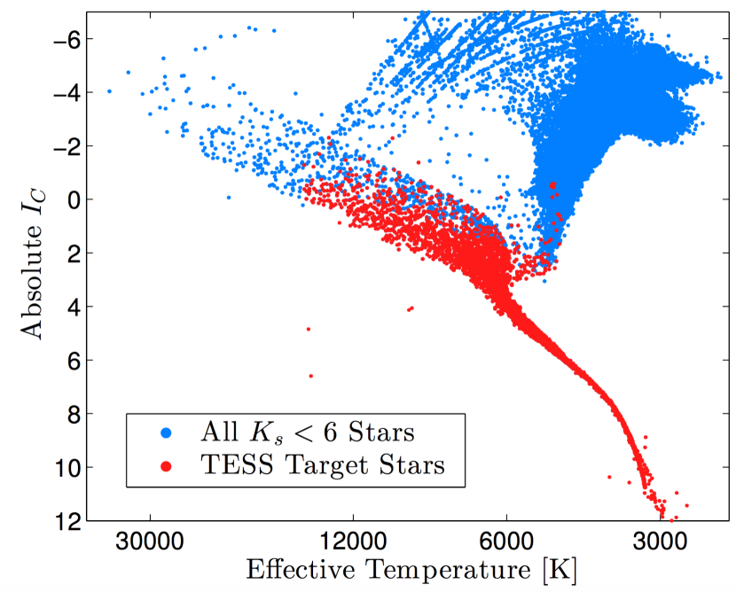
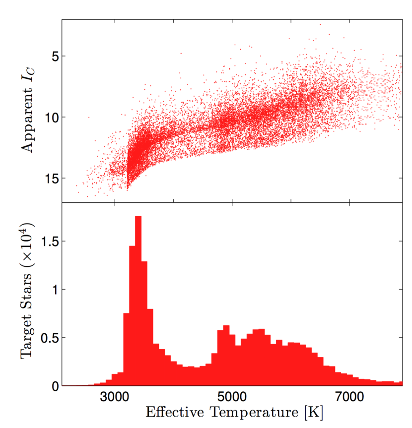
Figure 17 shows the distribution of target stars as a function of effective temperature, along with their apparent magnitudes. The distribution in effective temperature of the target stars is bimodal, with a sharp peak near 3400 K and a broader peak near 5500 K.
In reality, it will not be quite as straightforward to select the target stars for TESS. While proper-motion surveys (e.g., Lépine & Shara 2005) can readily distinguish red giants from dwarf stars, it is much more difficult to distinguish dwarfs from subgiant stars (Stassun et al., 2014). Ultimately, the selection of the TESS target stars may rely on parallaxes from the ongoing Gaia mission (Perryman et al., 2001). Errors in selecting the target stars might be mitigated by simply observing a larger number of stars at 2 min cadence. There is also the possibility of detecting transits in the full-frame images, which is described below.
6.8. Full-frame images
TESS will record and downlink a continuous sequence of full-frame images (FFIs) with an effective integration time of 30 min or shorter. Transiting planets can still be detected with 30 min sampling, but the longer integration time of the FFIs reduces the sensitivity to events with a short duration. Our simulation estimates the yield of transiting planets from the FFIs in the following fashion.
First, we identify all the transiting or eclipsing stars that are not among the pre-selected target stars. We assign to each system a random phase between the beginning of a 30 min window and the beginning of an eclipse. Next, we calculate the number of 30 min data points that are required to cover the transit or eclipse duration. The data points at the beginning and end of the series are omitted if they do not increase the signal-to-noise. Finally, we compute the effective depth of the transit or eclipse by averaging over all of the 30 min data points spanning the event. This step can reduce the depth because some of the data points include time outside of the transit or eclipse.
For transits with durations shorter than 1 hour, the 30-minute integration time of the FFIs causes the apparent transit duration to be lengthened and the apparent transit depth to become more shallow. However, the depths and durations of transits with longer durations are largely unaffected. The effects of time averaging on the uncertainties in transit parameters derived from light-curve fitting have been analyzed by Kipping (2010) and Price & Rogers (2014).
Our calculated detection threshold of 7.3 only ensures that no more than one statistical false positive is detected among the target stars. Since many more stars can be searched for transits in the FFIs, the number of statistical false-positives will be much greater than one if the same threshold is adopted.
7. SURVEY YIELD
Having calculated the SNR for each eclipsing or transiting system, we determine that a system is “detected” if the SNR in the phase-folded light curve and at least 2 transits or eclipse events are observed. We thereby produce a simulated catalog of detected planets and false positives.
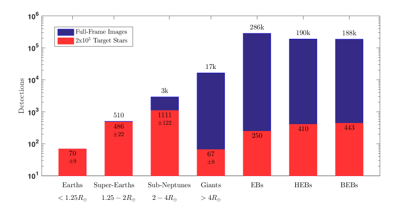
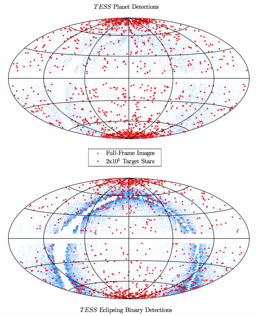
Figure 19 is a sky map in ecliptic coordinates of the simulated detections from one trial. Figure 18 shows the tallies for each class of planet and false positive. For the target stars, the yields we show are the average over five trials of the TESS mission; for the full-frame images, the yields are reported from a single trial since the computation time is much longer for this case.
The uncertainties that are printed in Figure 18 (for planets transiting the target stars) are based on the two primary sources of statistical uncertainty: the Poisson fluctuations in the number of detected planets and the statistical uncertainties in the planet occurrence rates (which are partly due to Poisson fluctuations in the Kepler sample of detected planets). We propagate the uncertainties in the occurrence rates by running 100 trials of the simulation. In each trial, the occurrence rates were perturbed by adding random Gaussian deviates to the quoted occurrence rate with the standard deviation set to the quoted uncertainty in the occurrence rate. In this way, the standard deviation in the number of planet detections across the 100 trials is essentially the quadrature sum of the Poisson fluctuations and the uncertainties propagated from the input occurrence rates. Poisson fluctuations are dominant for the categories of planets where the mean number of detected planets is small, such as habitable-zone planets.
The preceding calculations do not take into account systematic uncertainties. Among the sources of systematic uncertainty are the models of galactic structure and extinction, the stellar luminosity function, the stellar mass-radius-luminosity relations, and any bias in the planet occurrence rates. It is beyond the scope of this work to gauge the uncertainties in all of these inputs and the resulting impact on the planet yield. We can, however, make some general comments. We expect that the uncertainties in galactic structure and extinction will only be significant near the galactic plane, where it will be more difficult for TESS to detect planets due to crowding. Regarding the stellar luminosity function, it seems plausible that there are residual biases at the level of 10%, given that we found it necessary to adjust the model luminosity function by 30% across all absolute magnitudes to match the various sets of observational inputs. When coupled with uncertainties in the stellar mass-radius-luminosity relations, we would guess that the net impact on the planet detection statistics is at the level of 30%. Regarding biases in the planet occurrence rates upon which our simulation is based, it seems plausible that they are of the same order as the reported statistical errors, which have a median of 40% across all planetary sizes and periods. Therefore, the systematic uncertainties in the number of planet detections could be as large as 50%.
The number of planet detections from the full-frame images is sufficiently large that the systematic uncertainties almost certainly dominate over the statistical uncertainties, and therefore, the results should probably be valid to within a factor of two. For the same reason, we have not reported statistical uncertainties for the yields of astrophysical false positives. In addition to the systematic uncertainties mentioned above, there are additional uncertainties arising from the models for the stellar multiplicity fraction, mass ratio distribution, and eccentricity/period distributions. Our comparison to the Kepler eclipsing binary catalog indicates that for low galactic latitudes these uncertainties are of order of 80 (see Figure 10).
7.1. Transiting Planets
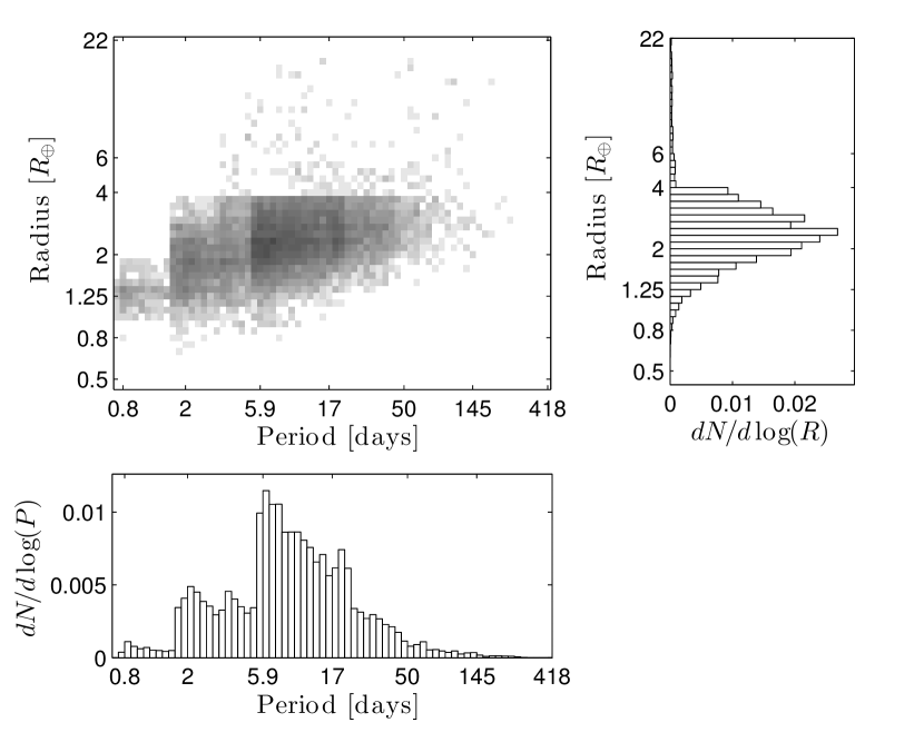
Total number of detections.—Based on five trials with the target stars, we expect TESS to find 709 planets smaller than 1.25 , 48622 planets in the range 1.25-2 , 1111122 planets in the range 2-4 , and 678 planets larger than 4 . Table 6 presents the catalog of planets from one of these five trials. Figure 20 shows the distribution of detected planets plotted on the radius-period plane, in the same fashion that the input planet occurrence rates were plotted in Figure 8.
The top panel of Figure 19 maps the simulated planet detections in ecliptic coordinates. Detections among the target stars (red points) are enhanced in the vicinity of the ecliptic poles because of the overlapping pointings they receive. Apart from that conspicuous feature, the detections are nearly uniformly distributed across the sky. The detections from stars that are only observed in the full-frame images (blue dots) show a strong enhancement near the galactic plane. This is due to the vast number of faint and distant stars around which giant planets can be detected.
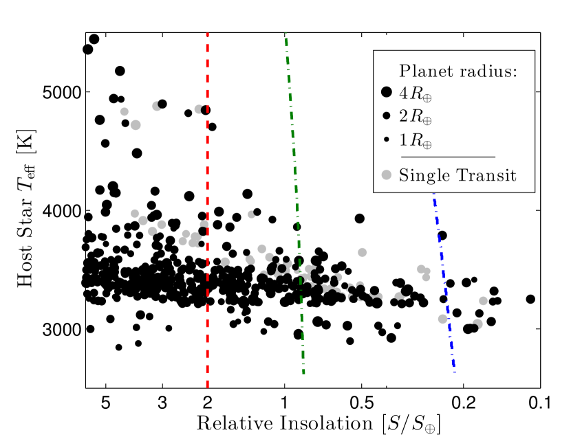
Habitable-zone planets.—Of the 556 planets smaller than 2 , a subset of 487 have a relative insolation on the range and are therefore near the habitable zone. We also expect a smaller subset of 144 to be within the more restricted zone defined by Kopparapu et al. (2013). This definition of the habitable zone extends approximately from , with the exact bounds depending on stellar effective temperature. Figure 21 shows the distribution of and for the simulated detections in the vicinity of the habitable zone. Because the sensitivity of TESS favors short periods, the potentially-habitable planets must orbit low-mass, cool stars with K. Furthermore, the yield of such planets depends strongly upon the definition of the inner edge of the habitable zone, but much less so upon the outer edge.
Small planets with measurable masses.—The smallest planets will be of particular interest for mass measurement since there are presently very few small (and potentially rocky) planets with measured masses and sizes. Among the 70 simulated planets smaller than 1.25 , the median period is 2.1 days, and the median stellar effective temperature is 3450 K. The median magnitude is 11.6.
Survey completeness.—The degree of completeness of the TESS survey can be assessed by comparing the simulated planet detections against the total number of transiting planets on the sky (as discussed in Section 4.1). Plotted in Figure 22 are the cumulative numbers of transiting planets as a function of the limiting apparent magnitude of the host star. We make the comparison for short-period planets around Sun-like and smaller stars for planets of different sizes as well as small planets near the HZ. For planets with , the completeness of the TESS survey is limited by instrumental noise. For planets with , the completeness is limited by the maximum number of target stars ().
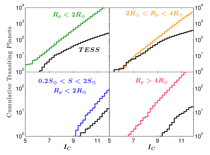
Diluting flux.—Whenever the photometric aperture contains flux from neighboring stars, the measured transit depth will be smaller than it would be if the star were observed in isolation. If this effect is not taken into account (by using observations with higher angular resolution), then the planet’s radius will be underestimated. The source of the “diluting flux” can be a star that is gravitationally bound to the target star, or it can be one or more completely unrelated stars along the same line-of-sight. In our simulation, we find that 12 of detected planets suffer dilution by more than , making them vulnerable to radius underestimation by . For 6 of planets, the radii could be underestimated by . We note that we do not consider cases of underestimated planet sizes to be “false positives”, in contrast to Fressin et al. (2013). Those authors considered the detection of transits with significant dilution to be a false positive because they were concerned with determining the occurrence rates of planets as a function of planet radius.
A separate scenario in which the transit depth can be diluted is when the transiting planet is actually orbiting a background star rather than the target star. Simulating these background transiting planets is a more computationally challenging problem which we conducted separately from the main simulations. We generated planets around the background stars represented by in “faint” star catalog and simulated the detection of the transiting planets blended with target stars. We found this type of transit detection to be very rare. Of the 2 target stars, we find that only 1 planet transiting a background star will be detectable with TESS. In the 30-minute full-frame images, approximately 70 such planets might be detected. The transit depths of these planets must be very deep to overcome the diluting flux of the brighter target star. In the simulations, the median radius of blended transiting planets is 17. Our conclusion is in agreement with those of Fressin et al. (2013), who found that transits of background stars are a less important source of detections than transits of planets around gravitationally bound companion stars (see their Figure 10).
Single-transit detections.—In a few notable cases, the SNR of a transit exceeds the threshold of , but only a single transit is observed. We expect 110 such planets to be detected with one transit. These are not counted as detections in the tallies given above, but they are included in Figure 21 as gray points. These planets have longer periods and lower equilibrium temperatures than the rest of the TESS sample. There may even be additional single-transit detections from planets with orbital periods exceeding one year, which we have not modeled at all. Although the periods will not be well-constrained using TESS data alone, and the probability of a “detection” being a statistical fluke is higher, it may still be worthwhile to conduct follow-up observations of these stars. The single-transit detections have a median planet size of 3 , a median orbital period of 30 days, and a median insolation of 1.9 .
7.2. False positives
Among the target stars, TESS detects 110333 eclipsing binary systems along with the transiting planets. The uncertainty in this figure is based only on the Poisson fluctuations; we acknowledge that the true uncertainty is likely to be significantly larger. Based on our comparison with the Kepler eclipsing binary catalog (see Section 4.2), the uncertainty may be as large as 80% for relatively low galactic latitudes.
The false-positives can be divided into the following cases:
-
1.
Eclipsing Binary (EB): The target star is an eclipsing binary with grazing eclipses. There are 250 16 detections of EBs.
-
2.
Hierarchical Eclipsing Binary (HEB): The target star is a triple or quadruple system in which one pair of stars is eclipsing. There are 410 20 detections of HEBs.
-
3.
Background Eclipsing Binary (BEB): The target star is blended with a background eclipsing binary. There are 443 20 detections of BEBs.
These tallies are also illustrated in Figure 18. The bottom panel of Figure 19 shows a sky map of the astrophysical false positives in the same coordinate system as the top panel. The surface density of false positives is a much stronger function of galactic coordinates than the density of planet detections, for binary eclipses are deeper than planetary transits and can be detected out to greater distances. The period and depth distributions of the eclipsing binary population is discussed in Section 8.6.
8. DISTINGUISHING FALSE POSITIVES FROM PLANETS
Experience has shown that the success of a transit survey depends crucially on the ability to distinguish transiting planets from astrophysical false positives. Our simulations suggest that for TESS, the number of astrophysical false positives will be comparable to the number of transiting planet detections. In many cases, it will be necessary (or at least desirable) to undertake ground-based follow-up observations to provide a definitive classification.
However, there will also be useful clues within the TESS data that a candidate is actually an eclipsing binary, even before any follow-up observations are undertaken. These clues are: (1) ellipsoidal variations, (2) secondary eclipses, (3) lengthy ingress and egress durations, or (4) centroid motion associated with the eclipse events. In this section, we investigate the prospects for using these four characteristics to identify false positives with TESS data alone. Specifically, we determine the number of cases, summarized in Table 5, for which any of these characteristics can be measured with an SNR of 5 or greater. This statistic indicates that the information will be available to help make the distinction between planet and false positive. The next step would be to combine all the measurable characteristics in a self-consistent manner and attempt to arrive at a definitive classification. This is a complex process which we have not attempted to model here.
8.1. Ellipsoidal Variations
The members of a close binary exert strong tidal gravitational forces on one another, causing their photospheres to deform into ellipsoids. These deformations lead to ellipsoidal variations in the light curve. A model for these photometric variations was presented by Morris & Naftilan (1993). Mazeh (2008) gave a simple expression for the dominant component, which has a period equal to half of the orbital period, and a semi-amplitude
| (24) |
where is the primary radius, is the orbital distance, is the orbital inclination, is the linear limb-darkening coefficient, is the gravity-darkening coefficient, and is the mass ratio. To estimate the amplitude of this effect for our simulated TESS detections, we adopt an appropriate value of for each star using the tables of Claret et al. (2012) and Claret et al. (2013), which come from the PHOENIX stellar models. For gravity darkening, we use a value of for all stars, which is thought to be appropriate for stars with convective envelopes (Lucy, 1967).
The formal detection limits for ellipsoidal variations are quite low because the signal is present throughout the entire light curve rather than being confined to eclipses of a narrower duration. Since the period and phase are fixed from the observed eclipses, we model the detection of the ellipsoidal variations as a cross-correlation of the light curve with a cosine function of the appropriate period. If the fractional uncertainty in flux of each data point is , and the total number of data points is , then the SNR of ellipsoidal variations is
| (25) |
Here, denotes the dilution of the target star in the photometric aperture, which is defined in Section 6.3. Due to this factor, ellipsoidal variations from BEBs are more difficult to detect since their eclipses are usually more diluted than EBs and HEBs. The factor of arises from the RMS value of a cosine function.
It seems likely that correlated noise will prevent the detection limit from averaging down to extremely low values as the duration of observations is extended. Somewhat arbitrarily, we require the semi-amplitude of the ellipsoidal variations to exceed 10 ppm, in addition to the criterion SNR, to be counted as “detectable.” We also require that the orbital period of the binary, which is twice the period of ellipsoidal variations, is shorter than one spacecraft orbit (13.6 days) out of concern that thermal or other variations of the satellite will induce systematic errors with a similar frequency. Under these detection constraints, shown in Figure 23, ellipsoidal variations are detected for 34 of the eclipsing binaries in the simulation. The majority of these are grazing-eclipse binaries rather than HEBs or BEBs. The results are summarized in the second column of Table 5.
8.2. Secondary Eclipse Detection
Another key difference between eclipsing binaries and transiting planets is that the secondary star in a binary is more luminous than a planetary companion. This distinction is somewhat blurred when comparing brown-dwarf and hot-Jupiter companions but is quite clear between ordinary stars and lower-mass planets. If the two stars in a binary have nearly the same surface brightness, then the depths of the primary and secondary eclipses will be indistinguishable. In this case, the system might appear to be a planet with an orbital period equal to half of the true orbital period of the binary. However, if the surface brightnesses of the stars differ and both eclipses are detected with a sufficiently high SNR, then the secondary eclipse can be distinguished from the primary eclipse and the system can be confidently classified as an eclipsing binary.
To estimate the number of cases for which the primary and secondary eclipses are distinguishable, we identify the simulated systems for which signal-to-noise of the secondary eclipses, SNR2, is , and the SNR in the difference between the primary and secondary eclipse depths, SNR1-2, is also . The latter quantity is calculated as
| (26) |
where denote the depths of the eclipses and denote the noise in the relative flux over the observed duration of each eclipse. Figure 24 shows the detectability of secondary eclipses by plotting SNR1-2 versus SNR2. The secondary eclipse can be distinguished from the primary eclipse for the systems that lie in the upper-right quadrant of the plot.
The results are also summarized in the third column of Table 5. A majority of the false positives have detectable secondary eclipses that are distinguishable in depth from the primary eclipses. The notable exceptions include the HEBs in which the eclipsing pair consists of equal-mass stars (). In such cases, and it is impossible to distinguish between primary and secondary eclipses. For the BEBs, the difficulty is that the eclipse depths are often strongly diluted and the secondary eclipses are not detectable. Most planets are too small and faint to produce detectable secondary eclipses in the TESS bandpass. In the simulations, the fraction of detected planets with detectable secondary eclipses is only 0.01.
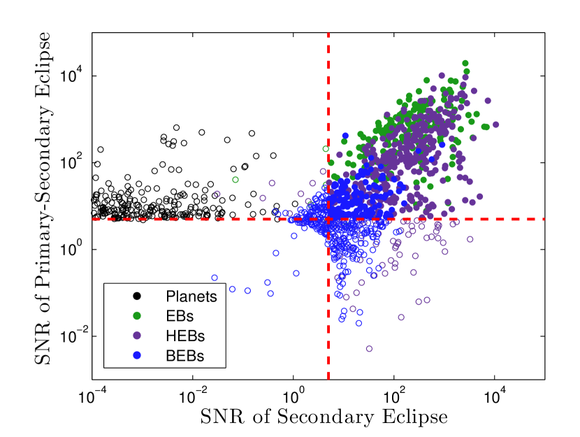
8.3. Ingress and Egress Detection
Eclipsing binaries can also be distinguished from transiting planets based on the more prolonged ingress and egress phases of stellar eclipses. As above, we adopt an SNR threshold of 5 for the ingress/egress phases to be detectable. The average “signal” during ingress and egress is half the maximum eclipse depth, and the “noise” is calculated for the combined durations of ingress and egress. In order to ensure that the ingress/egress can be temporally resolved, we require the duration of the ingress or egress to be more than twice as long as the duration of an individual data sample (2 min for the target stars and 30 min for the rest of the stars).
Since transiting planets generally have ingrees or egress phases lasting a few minutes, TESS will only be able to detect the ingress/egress for a small fraction (10%) of transiting planets observed with 2 min sampling. Only large planets observed in the 30 min. FFIs would have resolvable ingress/egress. However, the the ingress/egress phases of eclipsing binaries are more readily detectable.
We note that detection of the ingress/egress alone does not classify a signal as an eclipsing binary. One would next examine the period and shape of the eclipse signals to determine whether the radius of the eclipsing body is consistent with the observed depth.
Figure 25 illustrates the detection of ingress/egress for planets and false positives. The fourth column of Table 5 summarizes the results. Approximately 70% of the eclipsing binary systems that TESS detects among the target stars might be classified as false positives by virtue of a lengthy ingress or egress duration. For stars that are only observed at a 30 min cadence, this method is not as effective.
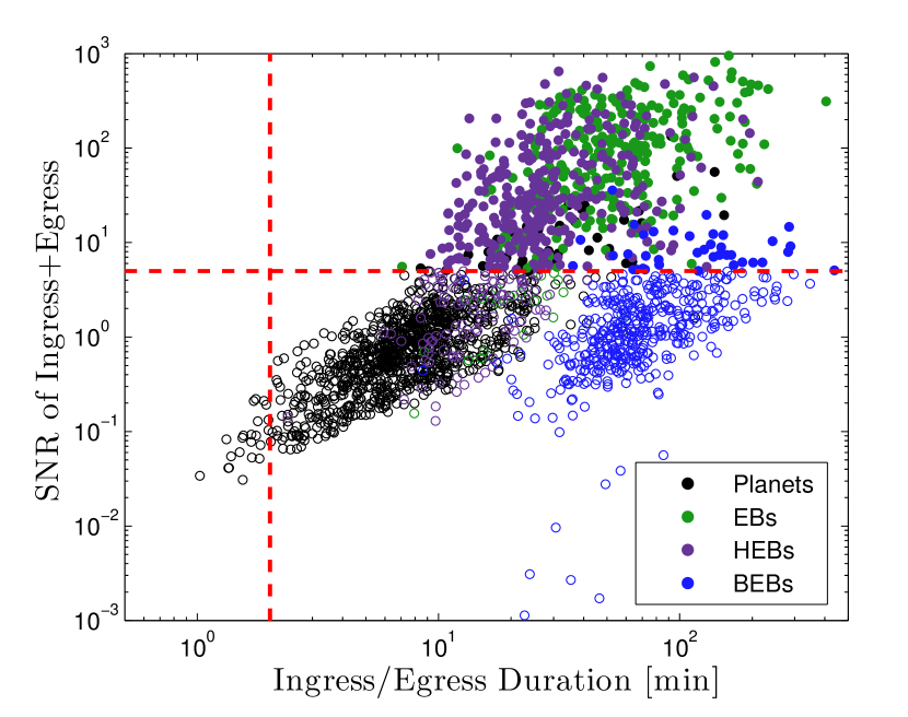
8.4. Centroid Motion
Another diagnostic of false positives, particularly background eclipsing binaries, is the centroid motion that accompanies the photometric variations. If there are detectable shifts in the centroid of the target star during transit or eclipse events, it is more likely that the target is a blended eclipsing binary rather than a transiting planet or an eclipse of the target star itself. Transits or eclipses of the target star can still have significant centroid motion if another bright star is blended with the target.
With real data, one could interpret the amplitude and direction of the measured centroid shift using the known locations of neighboring stars in order to determine the most likely source of the photometric variations. This is a complicated process to simulate, so we simply investigate the issue of the detecting the centroid shift. As verified in our simulations, the systems with detectable centroid shifts are much more likely to be false positives than transiting planets.
We simulate the detectability of centroid shifts by calculating the two-dimensional centroid (center-of-light) of the target star, and , within the synthetic images described in 6.2. We calculate the centroids both during and outside of the loss of light to find the magnitude and direction of the centroid shift. Next, we calculate the uncertainty in the centroid and , which stems from the photometric noise of each pixel. If each pixel has coordinates , and its photometric noise relative to the total flux is denoted by , then the noise propagates to the centroid measurement uncertainty through
| (27) |
In an analogous fashion to determining the optimal photometric aperture, we select the pixels that maximize the signal-to-noise ratio of the centroid measurement. Finally, we project the and centroid uncertainties in the direction of the centroid shift. The signal-to-noise ratio of the centroid measurement is the magnitude of the centroid shift divided by the centroid uncertainty projected in the direction of the centroid shift. We consider a centroid shift to be detectable if the signal-to-noise is 5 or greater.
In practice, the centroid measurement uncertainty could be much larger if the spacecraft jitter does not average down during the hour-long timescales of transits and eclipses. On the other hand, monotonic drifts in the spacecraft pointing during a transit or eclipse are less likely to impact the centroid measurement since the motion is common to all stars.
We find that centroid shifts can be detected for 69 of the BEBs and HEBs. These results are illustrated in Figure 26 and summarized in column 5 of Table 5. The BEBs have a higher fraction of detectable centroid shifts from the larger angular separations between the eclipsing system and the target star. Only 6 of planet transits produce a detectable centroid shift.
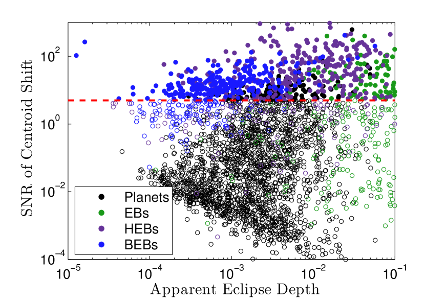
| aaMean number of each type of system that is detected. | Ellip.bbThe central four columns indicate the percentage of systems each with detectable ellipsoidal variations, secondary eclipses, ingress and egress, and centroid motion. | Sec. Ecl.bbThe central four columns indicate the percentage of systems each with detectable ellipsoidal variations, secondary eclipses, ingress and egress, and centroid motion. | In/EgressbbThe central four columns indicate the percentage of systems each with detectable ellipsoidal variations, secondary eclipses, ingress and egress, and centroid motion. | CentroidbbThe central four columns indicate the percentage of systems each with detectable ellipsoidal variations, secondary eclipses, ingress and egress, and centroid motion. | AnyccThe percentage of systems for which at least one of these four characteristics is detectable. | |
|---|---|---|---|---|---|---|
| EB | 250 | 79.9 | 80.2 | 92.5 | 31.7 | 98.6 |
| HEB | 410 | 43.1 | 73.4 | 74.5 | 71.2 | 93.0 |
| BEB | 443 | 0.8 | 30.4 | 10.9 | 69.1 | 74.1 |
| All FP | 1103 | 34.4 | 57.7 | 53.0 | 54.2 | 86.7 |
| PlanetsddSame, but restricted to planets larger or smaller than . For large planets the ingress/egress and the secondary eclipses are occasionally detectable. | ||||||
| 1667 | 0.0 | 0.0 | 1.9 | 6.3 | 1.9 | |
| 67 | 0.0 | 0.3 | 40.7 | 9.6 | 40.7 | |
8.5. Imaging
As shown in Table 5, the simulations suggest that blended eclipsing binaries are the type of false positive that is most difficult to identify based only on TESS data. Assuming that all of the false-positive tests described in the previous sections are applied, approximately 150 of the 110333 false positives would fail to be identified. The large majority (78) of these more stubborn cases are BEBs.
If archival images or catalogs do not reveal a system in the vicinity of a TESS target star that is consistent with any measurable centroid motion, then additional imaging is needed. An effective way to identify these BEBs is through ground-based imaging with higher angular resolution than the TESS cameras. A series of images spanning an eclipse could reveal which star (if any) is the true source of variations. Due to the large pixel scale of the TESS optics, it will not be difficult to improve upon the angular resolution with ground-based observations. Even modest contrast and a well-sampled PSF can resolve many ambiguous cases.
Figure 27 illustrates the requirements on angular resolution and contrast. For each BEB, we have plotted the angular separation and the -band magnitude difference between the BEB and the target star. Natural-seeing images with resolution would be sufficient to resolve all of the simulated BEBs. In more difficult cases, adaptive optics might be necessary to enable high contrast.
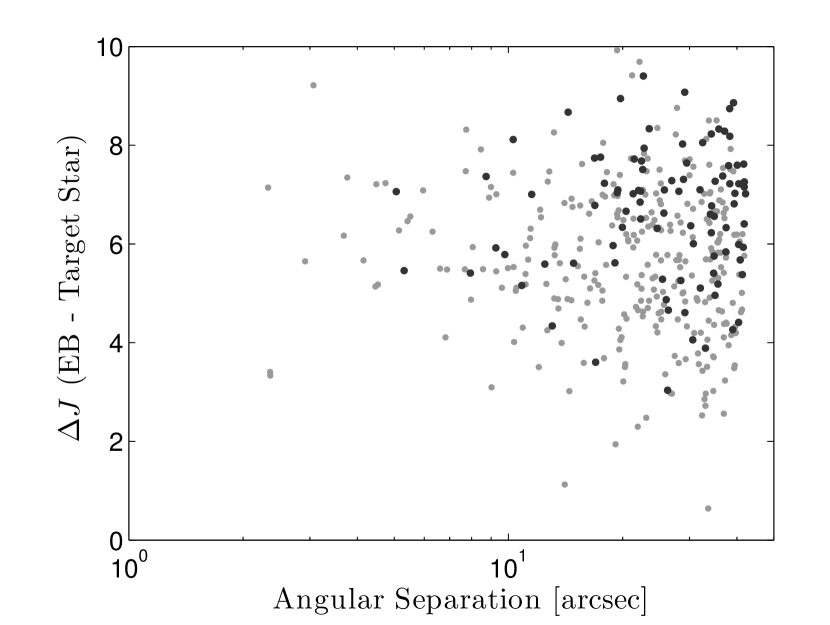
Figure 28 shows the photometric requirements to detect the planets as well as BEBs and other eclipsing systems for which the TESS photometry cannot distinguish whether the candidate is a false positive. We plot the eclipse depth against apparent system magnitude to indicate the photometric precision that is required of the facilities performing these observations.
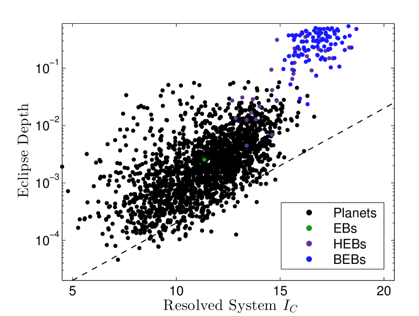
8.6. Statistical Discrimination
The false positives and transiting planets have significantly different distributions of orbital period, eclipse/transit depth, and galactic latitude. Therefore, the likelihood that a given source is a false positive can be estimated from the statistics of these distributions in addition to the characteristics described above that can be observed on a case-by-case basis.
Figure 29 shows the distributions of apparent period and apparent depth of the eclipses caused by transiting planets and false positives. Here, the “apparent period” is the period one would be likely to infer from the TESS photometry; if the secondary eclipse is detectable but not distinguishable from the primary eclipse, one would conclude that the period is half of the true orbital period. The “apparent depth” takes into account the dilution of an eclipse from background stars or, in the case of BEBs, the dilution from the target star.
These populations are seen to be quite distinct. Eclipsing binary systems tend to have larger depths and shorter periods than planets. Simply by omitting sources which have eclipse/transit depths 5% or periods 0.5 days, approximately 83 of the false positives among the target stars would be discarded.
The galactic latitude of the target also has a strong influence on the likelihood that a given source is a false positive. Figure 30 shows the fraction of detections that are due to planets, BEBs, and other false positives as a function of galactic latitude. Only the events with apparent depth 10% are included in this plot. For 10∘, the density of background stars is very high, and any observed eclipse is far more likely to be from a BEB than any other kind of eclipse. For 20∘, planets represent a majority over false positives. A weaker dependence on galactic latitude is seen for grazing-eclipse binaries and hierarchical eclipsing binaries.
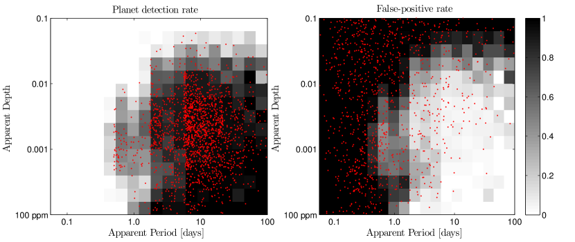
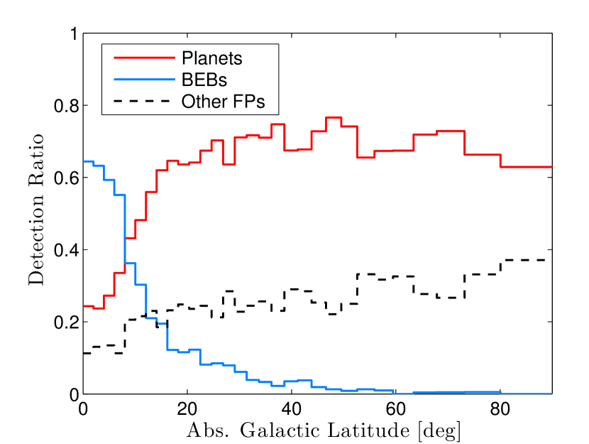
9. PROSPECTS FOR FOLLOW-UP OBSERVATIONS
We now turn to the prospects for follow-up observations to characterize the TESS transiting planets. As already discussed in Section 8.5, it is desirable to obtain transit light curves of the planetary candidates with a higher signal-to-noise than the TESS discovery. The photometry could be carried out with ground-based facilites or with upcoming space-based facilities such as CHEOPS (Fortier et al., 2014). This data can be used to look for transit timing variations and to improve our estimates of relative plantary radii.
Constraining the absolute planetary radii of the TESS planets will benefit from additional determinations of the radii of their host stars. Interferometric observations may be possible for the brightest and nearest host stars. For this reason, we report the stellar radii and distance moduli (in the “DM” column) of Table 6, allowing for estimation of angular diameters.
Asteroseismology can also be used to determine the radii of host stars if finely-sampled, high-precision photometry is available. Such data could come from the TESS data or the upcoming PLATO mission (Rauer et al., 2014). There is discussion of having TESS record the pixel values of the most promising targets for asteroseismology with a time sampling shorter than 2 min.
Next, we turn to the follow-up observations that TESS is designed to enable: radial-velocity observations to measure a planet’s mass and spectroscopic observations to detect and characterize a planet’s atmosphere.
9.1. Radial Velocity
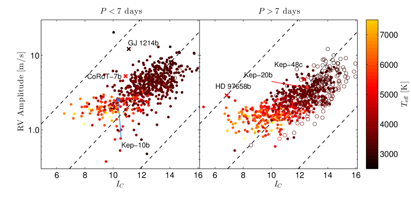
The TESS planets should be attractive targets for radial-velocity observations because the host stars will be relatively bright and their orbital periods will be relatively short. Both of these factors facilitate precise Doppler spectroscopy. To evaluate the detectability of the Doppler signal we assign masses to the simulated planets using the empirical mass-radius relation provided by Weiss et al. (2013). For , the planet mass is calculated as
| (28) |
and for , the mass is calculated as
| (29) |
This simple one-to-one relationship between mass and radius is used here for convenience. In reality, there is probably a distribution of planet masses for a given planet radius (see, e.g., Rogers 2014).
From the masses calculated here, we then find the radial-velocity semiamplitude , which is reported in Table 6. Figure 31 shows values of each planet detected in one trial as a function of the apparent magnitude of the host star. Because of the short periods, even planets smaller than 2 will produce a radial-velocity semiamplitude close to 1 m s-1, putting them within reach of current and upcoming spectrographs.
9.2. Atmospheric Characterization
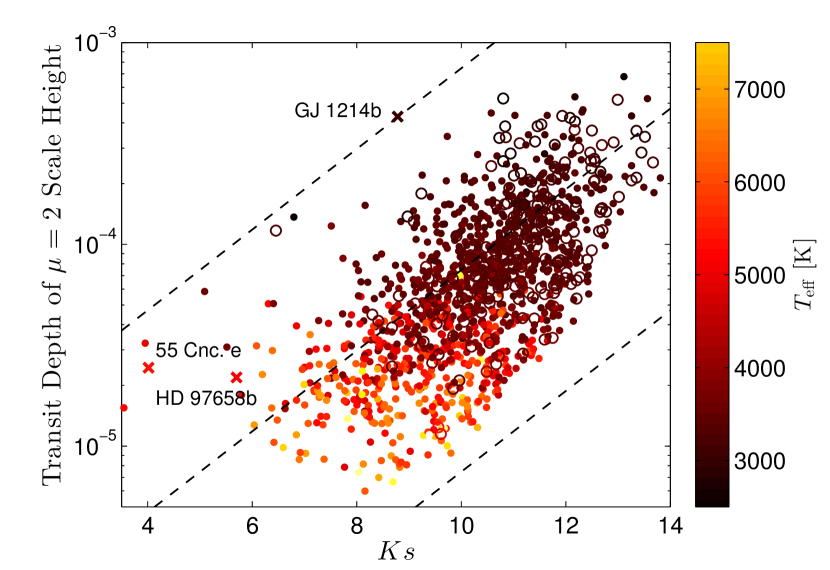
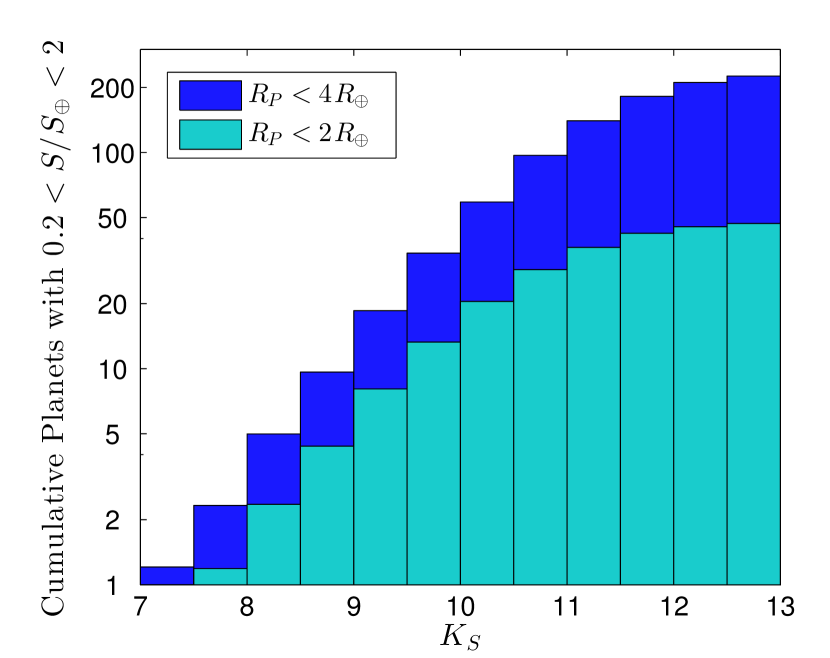
The composition of planetary atmospheres can be probed with transit spectroscopy. Such measurements can be carried out with space-based or balloon-based facilities, or even from ground-based facilities if the resolution is high enough to separate telluric features from stellar and planetary features. The enhanced sensitivity of TESS to transiting planets near the ecliptic poles will provide numerous targets for observations inside or near the continuous viewing zone of the James Webb Space Telescope. The prospects for follow-up with JWST have been detailed in Deming et al. (2009) and elsewhere. More specialized space missions, including FINESSE (Deroo et al., 2012) and EChO (Tinetti et al., 2012), have also been proposed to perform transit spectroscopy.
Here, we use the simulation results to explore the relative difficulty of transit spectroscopy of the TESS planets independent from the facility that is used to observe them. We compute a figure-of-merit , which is the fractional loss-of-light from an annulus surrounding the planet (with radius ) and a thickness equal to the scale height, :
| (30) |
The scale height is calculated from
| (31) |
where is the planet mass and is the proton mass. We calculate the temperature of the planet, , assuming it is in radiative equilibrium with zero albedo and isotropic re-radiation (see Eqn. 12). We assume a mean molecular weight of 2 amu, which corresponds to an atmosphere consisting purely of H2. In any other case, the atmospheric transit depth is reduced by a factor of . An Earth-like atmosphere would have amu, and a Venusian atmosphere would have amu.
Figure 32 shows for all of the detected planets in the simulation as a function of the apparent magnitude of the host star. For a molecular species to be identifiable, one must observe transits with a sensitivity on the order of both in and out of the absorption bands of that species. The detection of various species therefore depends on the depth of the absorption bands and the spectral resolution used to observe them. The presence of clouds and haze can reduce the observable thickness of the atmosphere.
Next, we look specifically at the number of planets with a relative insolation , placing them within or near the habitable zone. These planets are especially attractive targets for atmospheric spectroscopy because they may have atmospheres similar to that of the Earth, and may present “biomarkers” indicative of life. Such observations are most feasible for the planets with the brightest possible host stars. For that reason, we show in Figure 33 the cumulative distribution of apparent magnitudes of stars hosting planets with . With the statistical errors in the planet occurrence rates and Poisson fluctuations in the number of detected planets, between 2 and 7 planets with and have host stars brighter than .
Of particular interest for atmospheric spectroscopy with JWST are the planets that are located near the continuous-viewing zones of JWST, which will be centered on the ecliptic poles. A subset of 185 planets with and are found within 15∘ of the ecliptic poles. The brightest stars hosting these planets have 9.
10. SUMMARY
We have simulated the population of transiting planets and eclipsing binaries across the sky, and we have identified the subset of those systems that will be detectable by the TESS mission. To do so, we employed the TRILEGAL model of the galaxy to generate a catalog of stars covering 95 of the sky. We adjusted the modelled properties of those stars to align them with more recent observations and models of low-mass stars, the stellar multiplicity fraction as a function of mass, and the -band luminosity function of the galactic disk. We then added planets to these stars using occurrence rates derived from Kepler. Then, we modeled the process through which TESS will observe those stars and estimated the signal-to-noise ratio of the eclipse and transit events.
We report the statistical uncertainties in our tallies of detected planets arising from Poisson fluctuations and uncertainties in the planet occurrence rates. However, systematic errors in the occurrence rates, the luminosity function, and stellar properties are also significant. We also assumed that we can perfectly identify the best “target stars” for TESS to observe at the 2-min cadence. In reality, it is difficult to select these stars since subgiants can masquerade as main-sequence dwarfs. Parallaxes from Gaia could help determine the radii of TESS target stars more accurately, and examining the full-frame images will help find planets transiting the stars excluded from the 2-minute data.
The TESS planets will be attractive targets for follow-up measurements of transit properties, radial velocity measurements, and atmospheric transmission. Knowing the population of planets that TESS will detect allows the estimation of the follow-up resources that are needed, and it informs the design of future instruments that will observe the TESS planets. The simulations provide fine-grained statistical samples of planets and their properties which may be of interest to those who are planning follow-up observations or building instruments to enable such observations. Table 6 presents the results from one trial of the TESS mission. This catalog contains all the detected transiting planets from among the target stars that are observed at a 2 min cadence.
We look forward to the occasion, perhaps within 5-6 years, when TESS will have completed its primary mission and we are able to replace this simulated catalog with the real TESS catalog. This collection of transiting exoplanets will represent the brightest and most favorable systems for further study.
References
- Alonso et al. (2004) Alonso, R., Brown, T. M., Torres, G., et al. 2004, ApJ, 613, L153
- Andersen (1991) Andersen, J. 1991, A&A Rev., 3, 91
- Auvergne et al. (2009) Auvergne, M., Bodin, P., Boisnard, L., et al. 2009, A&A, 506, 411
- Bahcall & Soneira (1981) Bahcall, J. N., & Soneira, R. M. 1981, ApJS, 47, 357
- Bakos et al. (2004) Bakos, G., Noyes, R. W., Kovács, G., et al. 2004, PASP, 116, 266
- Basri et al. (2013) Basri, G., Walkowicz, L. M., & Reiners, A. 2013, ApJ, 769, 37
- Beatty & Gaudi (2008) Beatty, T. G., & Gaudi, B. S. 2008, ApJ, 686, 1302
- Bochanski et al. (2010) Bochanski, J. J., Hawley, S. L., Covey, K. R., et al. 2010, AJ, 139, 2679
- Borucki et al. (2010) Borucki, W. J., Koch, D., Basri, G., et al. 2010, Science, 327, 977
- Bouchy et al. (2005) Bouchy, F., Udry, S., Mayor, M., et al. 2005, A&A, 444, L15
- Boyajian et al. (2012) Boyajian, T. S., von Braun, K., van Belle, G., et al. 2012, ApJ, 757, 112
- Brown et al. (2011) Brown, T. M., Latham, D. W., Everett, M. E., & Esquerdo, G. A. 2011, AJ, 142, 112
- Burke et al. (2014) Burke, C. J., Bryson, S. T., Mullally, F., et al. 2014, ApJS, 210, 19
- Carter et al. (2008) Carter, J. A., Yee, J. C., Eastman, J., Gaudi, B. S., & Winn, J. N. 2008, ApJ, 689, 499
- Cardelli et al. (1989) Cardelli, J. A., Clayton, G. C., & Mathis, J. S. 1989, ApJ, 345, 245
- Chabrier (2001) Chabrier, G. 2001, ApJ, 554, 1274
- Charbonneau et al. (2000) Charbonneau, D., Brown, T. M., Latham, D. W., & Mayor, M. 2000, ApJ, 529, L45
- Charbonneau et al. (2009) Charbonneau, D., Berta, Z. K., Irwin, J., et al. 2009, Nature, 462, 891
- Chabrier et al. (2000) Chabrier, G., Baraffe, I., Allard, F., & Hauschildt, P. 2000, ApJ, 542, 464
- Claret et al. (2012) Claret, A., Hauschildt, P. H., & Witte, S. 2012, A&A, 546, AA14
- Claret et al. (2013) Claret, A., Hauschildt, P. H., & Witte, S. 2013, A&A, 552, AA16
- Cruz et al. (2007) Cruz, K. L., Reid, I. N., Kirkpatrick, J. D., et al. 2007, AJ, 133, 439
- Delfosse et al. (2004) Delfosse, X., Beuzit, J.-L., Marchal, L., et al. 2004, Spectroscopically and Spatially Resolving the Components of the Close Binary Stars, 318, 166
- Deming et al. (2009) Deming, D., Seager, S., Winn, J., et al. 2009, PASP, 121, 952
- Demory et al. (2011) Demory, B.-O., Gillon, M., Deming, D., et al. 2011, A&A, 533, AA114
- Deroo et al. (2012) Deroo, P., Swain, M. R., & Green, R. O. 2012, Proc. SPIE, 8442, 844241
- Dotter et al. (2008) Dotter, A., Chaboyer, B., Jevremović, D., et al. 2008, ApJS, 178, 89
- Dragomir et al. (2013) Dragomir, D., Matthews, J. M., Eastman, J. D., et al. 2013, ApJ, 772, LL2
- Dressing & Charbonneau (2013) Dressing, C. D., & Charbonneau, D. 2013, ApJ, 767, 95
- Dressing & Charbonneau (2015) Dressing, C. D., & Charbonneau, D. 2015, arXiv:1501.01623
- Duchêne & Kraus (2013) Duchêne, G., & Kraus, A. 2013, ARA&A, 51, 269
- Dumusque et al. (2014) Dumusque, X., Bonomo, A. S., Haywood, R. D., et al. 2014, ApJ, 789, 154
- Eggleton (2009) Eggleton, P. P. 2009, MNRAS, 399, 1471
- Eggleton & Tokovinin (2008) Eggleton, P. P., & Tokovinin, A. A. 2008, MNRAS, 389, 869
- Fabrycky et al. (2014) Fabrycky, D. C., Lissauer, J. J., Ragozzine, D., et al. 2014, ApJ, 790, 146
- Figueira et al. (2012) Figueira, P., Marmier, M., Boué, G., et al. 2012, A&A, 541, AA139
- Fortier et al. (2014) Fortier, A., Beck, T., Benz, W., et al. 2014, Proc. SPIE, 9143, 91432J
- Fressin et al. (2013) Fressin, F., Torres, G., Charbonneau, D., et al. 2013, ApJ, 766, 81
- Fuhrmann (1998) Fuhrmann, K. 1998, A&A, 338, 161
- Gaidos et al. (2014) Gaidos, E., Mann, A. W., Lépine, S., et al. 2014, MNRAS, 443, 2561
- Gautier et al. (2012) Gautier, T. N., III, Charbonneau, D., Rowe, J. F., et al. 2012, ApJ, 749, 15
- Gilliland et al. (2011) Gilliland, R. L., Chaplin, W. J., Dunham, E. W., et al. 2011, ApJS, 197, 6
- Girardi et al. (2000) Girardi, L., Bressan, A., Bertelli, G., & Chiosi, C. 2000, A&AS, 141, 371
- Girardi et al. (2005) Girardi, L., Groenewegen, M. A. T., Hatziminaoglou, E., & da Costa, L. 2005, A&A, 436, 895
- Girardi et al. (2012) Girardi, L., Barbieri, M., Groenewegen, M. A. T., et al. 2012, Red Giants as Probes of the Structure and Evolution of the Milky Way, 165
- Górski et al. (2005) Górski, K. M., Hivon, E., Banday, A. J., et al. 2005, ApJ, 622, 759
- Hatzes et al. (2011) Hatzes, A. P., Fridlund, M., Nachmani, G., et al. 2011, ApJ, 743, 75
- Hayes (1985) Hayes, D. S. 1985, Calibration of Fundamental Stellar Quantities, 111, 225
- Henry et al. (2006) Henry, T. J., Jao, W.-C., Subasavage, J. P., et al. 2006, AJ, 132, 2360
- Howell et al. (2014) Howell, S. B., Sobeck, C., Haas, M., et al. 2014, PASP, 126, 398
- Jenkins et al. (1996) Jenkins, J. M., Doyle, L. R., & Cullers, D. K. 1996, Icarus, 119, 244
- Jenkins et al. (2002) Jenkins, J. M., Caldwell, D. A., & Borucki, W. J. 2002, ApJ, 564, 495
- Jordi et al. (2006) Jordi, K., Grebel, E. K., & Ammon, K. 2006, A&A, 460, 339
- Kipping (2010) Kipping, D. M. 2010, MNRAS, 408, 1758
- Kopal (1979) Kopal, Z. 1979, Astrophysics and Space Science Library, 77, 21
- Kopparapu et al. (2013) Kopparapu, R. K., Ramirez, R., Kasting, J. F., et al. 2013, ApJ, 765, 131
- Kouwenhoven et al. (2007) Kouwenhoven, M. B. N., Brown, A. G. A., Portegies Zwart, S. F., & Kaper, L. 2007, A&A, 474, 77
- Kreidberg et al. (2014) Kreidberg, L., Bean, J. L., Désert, J.-M., et al. 2014, Nature, 505, 69
- van Leeuwen (2007) van Leeuwen, F. 2007, A&A, 474, 653
- Léger et al. (2009) Léger, A., Rouan, D., Schneider, J., et al. 2009, A&A, 506, 287
- Lépine & Shara (2005) Lépine, S., & Shara, M. M. 2005, AJ, 129, 1483
- Lucy (1967) Lucy, L. B. 1967, ZAp, 65, 89
- Marcy et al. (2014) Marcy, G. W., Isaacson, H., Howard, A. W., et al. 2014, ApJS, 210, 20
- Mazeh (2008) Mazeh, T. 2008, EAS Publications Series, 29, 1
- McCullough et al. (2005) McCullough, P. R., Stys, J. E., Valenti, J. A., et al. 2005, PASP, 117, 783
- Morris & Naftilan (1993) Morris, S. L., & Naftilan, S. A. 1993, ApJ, 419, 344
- Ofek (2008) Ofek, E. O. 2008, PASP, 120, 1128
- Perryman et al. (1997) Perryman, M. A. C., Lindegren, L., Kovalevsky, J., et al. 1997, A&A, 323, L49
- Pecaut & Mamajek (2013) Pecaut, M. J., & Mamajek, E. E. 2013, ApJS, 208, 9
- Pepper et al. (2003) Pepper, J., Gould, A., & Depoy, D. L. 2003, Acta Astronomica, 53, 213
- Pepper et al. (2007) Pepper, J., Pogge, R. W., DePoy, D. L., et al. 2007, PASP, 119, 923
- Price & Rogers (2014) Price, E. M., & Rogers, L. A. 2014, ApJ, 794, 92
- Perryman et al. (2001) Perryman, M. A. C., de Boer, K. S., Gilmore, G., et al. 2001, A&A, 369, 339
- Pickles (1998) Pickles, A. J. 1998, PASP, 110, 863
- Pollacco et al. (2006) Pollacco, D. L., Skillen, I., Collier Cameron, A., et al. 2006, PASP, 118, 1407
- Prša et al. (2011) Prša, A., Batalha, N., Slawson, R. W., et al. 2011, AJ, 141, 83
- Rauer et al. (2014) Rauer, H., Catala, C., Aerts, C., et al. 2014, Experimental Astronomy, 38, 249
- Reid et al. (2003) Reid, I. N., Cruz, K. L., Laurie, S. P., et al. 2003, AJ, 125, 354
- Raghavan et al. (2010) Raghavan, D., McAlister, H. A., Henry, T. J., et al. 2010, ApJS, 190, 1
- Reid et al. (2002) Reid, I. N., Gizis, J. E., & Hawley, S. L. 2002, AJ, 124, 2721
- Reid & Hawley (2005) Reid, I. N., & Hawley, S. L. 2005, New Light on Dark Stars: Red Dwarfs, Low-Mass Stars, Brown Dwarfs (Springer-Praxis)
- Ricker et al. (2015) Ricker, G. R., Winn, J. N., Vanderspek, R., Latham, D. W., et al. 2015, SPIE Journal of Astronomical Telescopes, Instruments, and Systems, 1, id.014003
- Rogers (2014) Rogers, L. A. 2014, arXiv:1407.4457
- Skrutskie et al. (2006) Skrutskie, M. F., Cutri, R. M., Stiening, R., et al. 2006, AJ, 131, 1163
- Slawson et al. (2011) Slawson, R. W., Prša, A., Welsh, W. F., et al. 2011, AJ, 142, 160
- Stassun et al. (2014) Stassun, K. G., Pepper, J. A., Paegert, M., De Lee, N., & Sanchis-Ojeda, R. 2014, arXiv:1410.6379
- Groenewegen et al. (2002) Groenewegen, M. A. T., Girardi, L., Hatziminaoglou, E., et al. 2002, A&A, 392, 741
- Tinetti et al. (2012) Tinetti, G., Beaulieu, J. P., Henning, T., et al. 2012, Experimental Astronomy, 34, 311
- Tremaine & Dong (2012) Tremaine, S., & Dong, S. 2012, AJ, 143, 94
- Van Grootel et al. (2014) Van Grootel, V., Gillon, M., Valencia, D., et al. 2014, ApJ, 786, 2
- Vanhollebeke et al. (2009) Vanhollebeke, E., Groenewegen, M. A. T., & Girardi, L. 2009, arXiv:0903.0946
- Weiss et al. (2013) Weiss, L. M., Marcy, G. W., Rowe, J. F., et al. 2013, ApJ, 768, 14
- Winn et al. (2011b) Winn, J. N., Albrecht, S., Johnson, J. A., et al. 2011, ApJ, 741, L1
- Winn et al. (2011a) Winn, J. N., Matthews, J. M., Dawson, R. I., et al. 2011, ApJ, 737, L18
- Winn (2011) Winn, J. N. 2011, in Exoplanets, edited by S. Seager. Tucson, AZ: University of Arizona Press, 2011, 526 pp. ISBN 978-0-8165-2945-2., p. 55-77
- Zheng et al. (2004) Zheng, Z., Flynn, C., Gould, A., Bahcall, J. N., & Salim, S. 2004, ApJ, 601, 500
| [∘] | [∘] | [days] | [m s-1] | [] | [K] | DM | Dil. | SNR | Mult. | |||||||
|---|---|---|---|---|---|---|---|---|---|---|---|---|---|---|---|---|
| 0.439 | 45.217 | 3.31 | 9.14 | 361.7 | 2.03 | 1.41 | 6531 | 8.47 | 7.97 | 7.63 | 7.41 | 5.00 | 1.00 | -4.87 | 16.8 | 1 |
| 0.480 | -66.204 | 2.19 | 14.20 | 2.1 | 3.11 | 0.32 | 3426 | 15.08 | 12.83 | 11.56 | 10.79 | 3.90 | 1.01 | -4.22 | 12.3 | 3 |
| 0.646 | 42.939 | 1.74 | 4.96 | 235.0 | 1.66 | 0.95 | 5546 | 10.12 | 9.35 | 8.81 | 8.41 | 4.95 | 1.00 | -4.64 | 7.5 | 0 |
| 0.924 | -26.065 | 1.48 | 2.16 | 1240.1 | 1.95 | 1.12 | 5984 | 8.06 | 7.42 | 6.98 | 6.67 | 3.65 | 1.00 | -4.50 | 8.4 | 0 |
| 1.314 | -24.954 | 2.29 | 9.75 | 5.9 | 2.95 | 0.42 | 3622 | 14.19 | 12.15 | 10.99 | 10.19 | 4.10 | 1.00 | -4.44 | 8.6 | 2 |
| 1.384 | 10.606 | 2.32 | 13.99 | 2.1 | 3.32 | 0.32 | 3425 | 15.04 | 12.79 | 11.52 | 10.74 | 3.85 | 1.07 | -3.50 | 7.8 | 2 |
| 1.783 | -71.931 | 3.29 | 8.42 | 4.5 | 5.23 | 0.34 | 3444 | 15.29 | 13.06 | 11.79 | 11.02 | 4.25 | 1.00 | -4.39 | 26.4 | 2 |
| 1.789 | -9.144 | 2.81 | 5.62 | 2.6 | 9.15 | 0.17 | 3228 | 15.05 | 12.52 | 11.13 | 10.36 | 1.85 | 2.28 | -4.41 | 28.7 | 3 |
| 1.948 | -16.995 | 17.15 | 1.34 | 10164.5 | 16.03 | 2.11 | 6668 | 7.51 | 7.05 | 6.72 | 6.53 | 5.00 | 1.00 | -4.42 | 457.4 | 2 |
| 2.172 | -15.533 | 4.80 | 17.14 | 341.2 | 2.10 | 2.11 | 6668 | 7.51 | 7.05 | 6.72 | 6.53 | 5.00 | 1.00 | -4.68 | 13.1 | 2 |
| 4.071 | 9.507 | 1.97 | 11.45 | 1.5 | 4.09 | 0.22 | 3300 | 14.96 | 12.55 | 11.21 | 10.44 | 2.65 | 1.00 | -4.50 | 17.7 | 2 |
| 4.634 | -23.500 | 4.71 | 5.17 | 116.3 | 4.60 | 0.80 | 5000 | 9.52 | 8.54 | 7.85 | 7.32 | 3.35 | 1.00 | -4.68 | 64.0 | 0 |
| 4.788 | 78.625 | 1.56 | 0.62 | 71.2 | 8.92 | 0.22 | 3283 | 15.94 | 13.50 | 12.14 | 11.38 | 3.50 | 1.00 | -4.43 | 16.9 | 2 |
| 5.322 | -55.554 | 2.85 | 18.16 | 2.4 | 3.01 | 0.41 | 3592 | 14.23 | 12.15 | 10.98 | 10.18 | 4.00 | 1.00 | -4.46 | 15.5 | 2 |
| 5.704 | 50.726 | 2.24 | 2.75 | 308.3 | 2.82 | 0.80 | 5188 | 11.28 | 10.40 | 9.77 | 9.28 | 5.35 | 1.01 | -4.67 | 10.6 | 2 |
| 5.951 | -28.675 | 3.75 | 17.75 | 4.3 | 3.46 | 0.50 | 3844 | 11.73 | 9.94 | 8.89 | 8.08 | 2.55 | 1.00 | -4.29 | 52.5 | 1 |
| 6.166 | 32.455 | 1.11 | 0.79 | 53.4 | 2.95 | 0.22 | 3304 | 14.81 | 12.41 | 11.08 | 10.32 | 2.65 | 1.00 | -3.50 | 8.5 | 2 |
| 6.521 | -4.048 | 1.53 | 7.51 | 4.8 | 2.78 | 0.32 | 3435 | 13.66 | 11.43 | 10.17 | 9.41 | 2.50 | 1.00 | -3.49 | 8.3 | 2 |
| 6.662 | -79.377 | 2.31 | 1.89 | 45.5 | 5.48 | 0.40 | 3551 | 14.42 | 12.30 | 11.10 | 10.31 | 4.00 | 1.00 | -3.49 | 19.9 | 0 |
| 7.592 | -79.924 | 7.72 | 3.92 | 320.7 | 7.41 | 0.91 | 5623 | 11.06 | 10.32 | 9.79 | 9.40 | 5.85 | 1.00 | -4.54 | 96.5 | 1 |
| 8.071 | -77.185 | 1.49 | 1.02 | 887.9 | 3.50 | 0.70 | 5030 | 8.00 | 7.05 | 6.40 | 5.85 | 1.60 | 1.00 | -4.74 | 40.7 | 1 |
| 8.396 | -53.966 | 2.38 | 5.59 | 6.8 | 4.55 | 0.31 | 3442 | 14.14 | 11.91 | 10.66 | 9.89 | 2.95 | 1.25 | -3.60 | 20.3 | 3 |
| 8.919 | 67.419 | 2.94 | 29.94 | 1.3 | 2.61 | 0.42 | 3611 | 13.33 | 11.30 | 10.14 | 9.35 | 3.20 | 1.09 | -3.69 | 18.1 | 1 |
| 9.843 | -11.832 | 2.82 | 6.28 | 62.9 | 2.98 | 0.69 | 4819 | 11.69 | 10.60 | 9.88 | 9.26 | 4.90 | 1.00 | -4.85 | 17.2 | 0 |
| 10.467 | -40.605 | 1.71 | 15.14 | 1.3 | 2.83 | 0.26 | 3359 | 14.51 | 12.18 | 10.87 | 10.11 | 2.70 | 1.02 | -3.49 | 9.1 | 1 |
| 10.551 | -27.297 | 3.60 | 5.99 | 283.9 | 2.96 | 1.04 | 5970 | 9.85 | 9.21 | 8.76 | 8.44 | 5.25 | 1.00 | -4.52 | 22.5 | 0 |
| 11.067 | -52.752 | 2.40 | 17.18 | 0.9 | 4.35 | 0.22 | 3287 | 15.54 | 13.10 | 11.74 | 10.98 | 3.10 | 1.00 | -4.32 | 17.8 | 1 |
| 11.145 | 29.347 | 2.43 | 8.66 | 13.3 | 2.80 | 0.53 | 3948 | 12.80 | 11.09 | 10.08 | 9.27 | 3.95 | 1.01 | -4.46 | 13.8 | 2 |
| 11.145 | -49.044 | 1.51 | 8.12 | 6.4 | 2.27 | 0.39 | 3557 | 13.67 | 11.56 | 10.37 | 9.58 | 3.25 | 1.03 | -4.45 | 10.7 | 1 |
| 11.207 | 37.355 | 2.64 | 1.98 | 28.9 | 7.02 | 0.32 | 3437 | 14.67 | 12.43 | 11.18 | 10.40 | 3.55 | 1.02 | -4.01 | 22.6 | 3 |
| 11.547 | -44.670 | 5.26 | 39.43 | 56.6 | 1.90 | 1.47 | 6577 | 8.65 | 8.16 | 7.82 | 7.62 | 5.30 | 1.00 | -4.01 | 14.5 | 0 |
| 11.909 | -67.746 | 3.67 | 4.78 | 216.5 | 3.69 | 0.84 | 5598 | 11.69 | 10.94 | 10.40 | 10.00 | 6.25 | 1.01 | -3.77 | 20.4 | 0 |
| 12.015 | 74.529 | 3.85 | 1.85 | 11.8 | 17.24 | 0.17 | 3225 | 16.89 | 14.36 | 12.95 | 12.18 | 3.75 | 1.10 | -3.49 | 45.8 | 3 |
| 12.085 | -51.662 | 11.96 | 40.02 | 16.1 | 4.97 | 0.99 | 5598 | 10.31 | 9.55 | 9.02 | 8.63 | 5.25 | 1.01 | -4.74 | 169.9 | 0 |
| 12.261 | -60.310 | 2.12 | 10.35 | 3.4 | 3.19 | 0.33 | 3467 | 13.88 | 11.68 | 10.44 | 9.67 | 2.90 | 1.00 | -3.53 | 13.3 | 2 |
| 12.320 | 75.640 | 6.92 | 5.25 | 513.2 | 5.25 | 1.20 | 6295 | 10.12 | 9.57 | 9.18 | 8.91 | 6.10 | 1.54 | -4.12 | 64.3 | 1 |
| 12.410 | -10.212 | 2.97 | 6.84 | 2.2 | 8.51 | 0.18 | 3230 | 16.63 | 14.10 | 12.70 | 11.93 | 3.60 | 1.00 | -4.39 | 9.0 | 0 |
| 12.640 | -53.861 | 1.73 | 2.40 | 20.9 | 4.48 | 0.31 | 3442 | 14.14 | 11.91 | 10.66 | 9.89 | 2.95 | 1.00 | -3.95 | 17.7 | 3 |
| 12.928 | -13.886 | 12.98 | 6.03 | 8419.9 | 5.13 | 2.50 | 10593 | 6.03 | 6.14 | 6.15 | 6.21 | 5.55 | 1.00 | -4.16 | 61.4 | 1 |
| 12.974 | 58.302 | 2.77 | 13.71 | 422.9 | 1.35 | 1.56 | 7603 | 9.02 | 8.77 | 8.57 | 8.48 | 6.45 | 1.06 | -4.50 | 7.9 | 1 |
| 13.048 | 74.712 | 1.47 | 1.06 | 81.4 | 5.18 | 0.36 | 3490 | 15.02 | 12.84 | 11.60 | 10.82 | 4.25 | 1.30 | -3.61 | 7.9 | 2 |
| 13.408 | 27.048 | 3.21 | 11.65 | 84.2 | 2.21 | 0.96 | 5689 | 10.53 | 9.81 | 9.30 | 8.93 | 5.50 | 1.01 | -4.84 | 13.2 | 1 |
| 13.494 | -57.211 | 1.98 | 19.54 | 2.3 | 2.08 | 0.42 | 3606 | 14.03 | 11.97 | 10.80 | 10.01 | 3.90 | 1.00 | -4.53 | 8.0 | 3 |
| 13.690 | -81.593 | 1.85 | 2.20 | 15.3 | 6.25 | 0.24 | 3324 | 14.95 | 12.57 | 11.24 | 10.48 | 2.85 | 1.15 | -3.84 | 29.3 | 3 |
| 13.824 | -20.209 | 1.05 | 15.96 | 0.6 | 1.16 | 0.16 | 3228 | 14.83 | 12.30 | 10.91 | 10.15 | 1.60 | 1.00 | -3.96 | 8.3 | 1 |
| 14.214 | 79.814 | 1.06 | 0.50 | 659.2 | 1.50 | 0.55 | 3996 | 12.87 | 11.21 | 10.21 | 9.40 | 4.20 | 1.05 | -4.10 | 7.9 | 3 |
| 14.313 | 32.413 | 2.29 | 5.80 | 7.6 | 4.23 | 0.34 | 3470 | 12.33 | 10.15 | 8.92 | 8.15 | 1.40 | 1.00 | -4.54 | 46.1 | 2 |
| 14.807 | -14.485 | 1.99 | 12.55 | 0.6 | 5.39 | 0.16 | 3027 | 14.98 | 12.76 | 11.10 | 10.32 | 1.45 | 1.00 | -3.53 | 19.7 | 1 |
| 15.256 | 48.530 | 2.27 | 7.68 | 4.4 | 3.93 | 0.31 | 3435 | 14.47 | 12.23 | 10.98 | 10.21 | 3.25 | 1.21 | -3.70 | 15.1 | 2 |
| 15.926 | 75.902 | 1.94 | 5.06 | 333.5 | 1.72 | 1.05 | 5888 | 8.68 | 8.02 | 7.56 | 7.23 | 4.05 | 1.00 | -4.64 | 16.7 | 2 |
Note. — This catalog is based on one realization of the Monte Carlo simulation. The detections are drawn from the target stars that are observed with a 2 min cadence. The larger sample of detections from stars that are only observed in full-frame images is not provided here. The entirety of this table is available electronically; only the first 50 lines are shown here to illustrate its form and content.