A Constructive Spatio-Temporal Approach to Modeling Spatial Covariance

Abstract

I present an approach for modeling areal spatial covariance by considering the stationary distribution of a spatio-temporal Markov random walk. This stationary distribution corresponds to an intrinsic simultaneous autoregressive (SAR) model for spatial correlation, and provides a principled approach to specifying areal spatial models when a spatio-temporal generating process can be assumed. I apply the approach to a study of spatial genetic variation of trout in a stream network in Connecticut, USA, and a study of crime rates in neighborhoods of Columbus, OH, USA.

Keywords: SAR models, Diffusion, Autoregressive models.

1 Introduction

Almost all spatial data can be viewed as arising from a spatio-temporal generating process. For example, a spatial survey of infectious disease prevalence is a snapshot of a dynamic epidemic process occuring in space and time. Similarly, spatial genetic data are the result of spatio-temporal dispersal, mating, and survival processes at the population level. When these spatial processes are observed at multiple successive time points, the known science behind the spatio-temporal process is often used to motivate a spatio-temporal statistical model (e.g., Wikle & Hooten, 2010; Cressie & Wikle, 2011).

In contrast, consider the case of “spatial” data, where only one temporal realization of the spatio-temporal process is observed. In this case, spatial autocorrelation is often modeled by including a spatial random effect (e.g., Diggle & Ribeiro, 2007) in the fitted statistical model. The prior distribution for this spatial random effect is almost always modeled semiparametrically using a Gaussian process model with covariance function chosen based on the support of the data, irrespective of the spatio-temporal generating process. For example, when the spatial data are point-referenced, the Matern class of covariance functions (e.g., Cressie, 1993) are often used, while if the spatial data have areal or lattice support, then either conditional autoregressive (CAR; e.g., Besag, 1974; Besag & Kooperberg, 1995; Rue & Held, 2005) or simultaneous autoregressive (SAR: e.g., Wall, 2004; Cressie & Wikle, 2011) models are common. In either case, the choice of prior distribution for the spatial random effect is almost always made based solely on the support of the data, without consideration of an underlying generating process.

Spatial data are poor in information relative to spatio-temporal data; however, we are increasingly able to collect large amounts of spatial data. The increased information present in large spatially-correlated data provides an opportunity for more realistic modeling of spatial covariance than has been possible in the past. Additionally, recent recognition of the potential for spatial confounding (Hodges & Reich, 2010; Paciorek, 2010; Hughes & Haran, 2013; Hanks, Schliep, Hooten & Hoeting, 2015) highlights the need to choose a spatial model with care, as the structure of a spatially-correlated random effect can influence inference on fixed effects.

I propose a general constructive approach to modeling spatial correlation based on considering the stationary distribution of a spatio-temporal generating process. This spatio-temporal generating process can either be specified based on scientific knowledge, or can be thought of simply as a device to construct a spatial correlation with desired properties, such as anisotropy and nonstationarity. In Section 2, I describe the proposed general approach, and link it to current spatial models for continuous (geostatistical) random fields. In Section 3, I focus on areal spatial models and show that the stationary distribution for a spatio-temporal random walk model results in a spatial SAR model, which provides a principled approach for choosing areal neighbors and SAR weights when spatial data can be seen as arising from a spatio-temporal random walk. In Section 4, I use this development to model spatial genetic data based on a spatio-temporal random walk generating process. I apply this model to genetic data collected from trout in the Jefferson-Hill Spruce Brook in Connecticut, USA. In Section 5 I present a second example by modeling crime rates for areal neighborhoods in Columbus, Ohio, USA. This second example illustrates how a spatio-temporal generating process can be used to jointly model fixed and random spatial effects. In Section 6 I close with discussion of the proposed approach.

2 A Constructive Spatio-Temporal Approach to Modeling Spatial Covariance

The proposed approach is as follows.

1. Define a deterministic spatio-temporal generating model for the spatio-temporal process $\mathbf{y}(s,t)$, where $s$ indexes space and $t$ indexes time

   $$\frac{\partial}{\partial t}\mathbf{y}(s,t)=\mathcal{F}\left(\mathbf{y}(s,t)\right).$$ (1)

   For example, $\mathcal{F}$ could be a differential operator (e.g., $\frac{\partial^{2}}{\partial s^{2}}$) in which case (1) is a partial differential equation (PDE).

2. Drive the spatio-temporal process defined by (1) with time-homogeneous spatial noise $\mathbf{W}(s)$

   $$\frac{\partial}{\partial t}\mathbf{y}(s,t)=\mathcal{F}\left(\mathbf{y}(s,t)\right)+\mathbf{W}(s)\quad,\quad\mathbf{W}(s)\sim N(\cdot,\cdot).$$ (2)

   The process (2) is now a random (stochastic) process in contrast to (1), which is deterministic.

3. The stationary distribution $\boldsymbol{\pi}(s)=\lim_{t\rightarrow\infty}\mathbf{y}(s,t)$ of (2) provides a spatial model capturing the dynamics of the spatio-temporal process.

   $$\frac{\partial}{\partial t}\mathbf{y}(s,t)=0\quad\Rightarrow\quad\mathcal{F}\left(\boldsymbol{\pi}(s)\right)=-\mathbf{W}(s)$$ (3)

Solving (3) for the stationary distribution $\boldsymbol{\pi}(s)$ can be done analytically in some cases, but in many others a numerical approximation will be required.

2.1 Spatio-Temporal Generating Models for Continuous-Space Spatial Models

I first consider this approach in the context of continuous-space processes, and restrict attention to spatial processes in $\mathcal{R}^{2}$, with the two dimensions $\mathbf{s}=(x_{1},x_{2})$. The generalization to higher (or lower) spatial dimensions is straightforward (Lindgren et al., 2011). The most common spatial covariance function used in continuous space is the Matern class, with covariance function given by

$$\text{cov}(\mathbf{s}_{i},\mathbf{s}_{j})=\sigma^{2}\frac{1}{\Gamma(\nu)2^{\nu-1}}\left(\sqrt{2\nu}\frac{d_{ij}}{\phi}\right)^{\nu}K_{\nu}\left(\sqrt{2\nu}\frac{d_{ij}}{\phi}\right)$$

where $d_{ij}=\sqrt{(x_{i1}-x_{j1})^{2}+(x_{i2}-x_{j2})^{2}}$ is the Euclidean distance between the spatial locations of the $i$-th and $j$-th observations, $\sigma^{2}$ is the partial sill parameter, $\nu$ is the Matern smoothness parameter, $\phi$ is a range parameter, and $K_{\nu}(\cdot)$ is the modified Bessel function of the second kind (e.g., Cressie, 1993).

As a special case of the constructive spatio-temporal approach proposed in the previous section, consider the random partial differential equation

$$\frac{\partial}{\partial t}\mathbf{y}(x_{1},x_{2},t)=(\Delta-\kappa^{2})^{\alpha/2}\mathbf{y}(x_{1},x_{2},t)+\mathbf{W}(x_{1},x_{2}),$$ (4)

where $\Delta=\frac{\partial^{2}}{\partial x_{1}^{2}}+\frac{\partial^{2}}{\partial x_{2}^{2}}$ is the Laplacian and $\mathbf{W}(x_{1},x_{2})$ is time-homogeneous spatial Gaussian white noise. Note that while equation (4) has been termed a stochastic partial differential equation (SPDE; Lindgren et al., 2011), I follow Kloeden & Platen (1992) and reserve SPDE to refer to a differential equation model driven by noise which varies over time (e.g., $\mathbf{W}(x_{1},x_{2},t)$ could be a spatial Wiener process), while a random partial differential equation (RPDE) is a differential equation driven by time-homogeneous noise, as in (2) and (4).

The stationary distribution of (4) satisfies the RPDE

$$(\kappa^{2}-\Delta)^{\alpha/2}\boldsymbol{\pi}(x_{1},x_{2})=\mathbf{W}(x_{1},x_{2}),$$

whose solution is a random field of the Matern class (Whittle, 1954; Lindgren et al., 2011). As a concrete example, consider (4) when $\kappa^{2}=0$ and $\alpha=2$

$$\frac{\partial}{\partial t}\mathbf{y}(x_{1},x_{2},t)=\left(\frac{\partial^{2}}{\partial x_{1}^{2}}+\frac{\partial^{2}}{\partial x_{2}^{2}}\right)\mathbf{y}(x_{1},x_{2},t)+\mathbf{W}(x_{1},x_{2}).$$ (5)

The spatio-temporal generating process (5) is a two-dimensional diffusion with time-homogeneous spatial sources and sinks defined by $\mathbf{W}(s)$. The corresponding stationary spatial distribution is an intrinsic Matern random field with smoothness parameter $\nu=2$ (See Lindgren et al., 2011, for details).

The novelty introduced in this section is the temporal aspect of the RPDE approach, which is not necessary to use spatial models motivated by RPDEs. However, the interpretation of spatial models as stationary distributions of spatio-temporal RPDEs opens up the possibility of scientific modeling of spatial random effects when a spatio-temporal generating process, such as diffusion (5), can be assumed. Having shown how the Matern class of spatial models can be seen as the stationary distributions of the continuous space spatio-temporal RPDE (4), I now consider spatio-temporal models with discrete (areal) spatial support.

3 Discrete Space Random Walk Models for Spatial Covariance

Lindgren et al. (2011) consider discrete (areal) spatial models in the context of numerically approximating the solution to the RPDE (4) using a finite element basis set. Approximating a continuous spatial random field with a finite element approximation leads to increases in computational efficiency, as the finite element basis solution results in a Gaussian Markov random field (GMRF) with sparse precision matrix.

Instead of continuous spatial effects, consider modeling areal spatial processes directly. That is, consider modeling a spatial random effect $\mathbf{y}=[y_{1},y_{2},\ldots,y_{n}]^{\prime}$ on $n$ spatial locations which constitute the full spatial support of the random effect. While both CAR and SAR models have been used extensively to model spatial autocorrelation in areal spatial models, there is little in the way of guidance on when to use one or the other, and little guidance on how to define the neighborhood structure that defines the CAR and SAR models (e.g., Wall, 2004; Assunção & Krainski, 2009).

By considering a Markov random walk on a discrete spatial support, I will first derive a population-level diffusion RPDE based on a large-population approximation to the spatial movements of many individuals. I will then show that the stationary distribution to this RPDE is a SAR model. This result will then be used in Section 5 and Section 6 to propose spatial covariance models based on population-level spatial random walk or diffusion processes.

3.1 Population-level Markov random walks

Let $\mathbf{G}=(\mathbf{V},\mathbf{E})$ be a graph with vertices $\mathbf{V}=\{V_{1},V_{2},\ldots,V_{M}\}$ and directed edges $\mathbf{E}=\{\alpha_{ij},i=1,2,\ldots,M;j=1,2,\ldots,M\}$. In particular, consider the case where $\alpha_{ij}$ is the exponential rate at which a random walker in node $i$ transitions to node $j$. As in a standard continuous-time Markov chain (CTMC) model for a random walk, the time $T_{i}$ spent by a random walker in node $i$ before transitioning to any other node is exponentially-distributed with rate $\alpha_{i}=\sum_{k=1}^{n}\alpha_{ik}$.

Consider population-level processes on the graph $\mathbf{G}$ in which there are $N$ members of the population, all behaving as a random walk. If there are $n_{i}(t)$ individuals at node $i$ and time $t$, then the rate at which individuals move from node $i$ to node $j$ is given by $n_{i}\alpha_{ij}$. Following Kurtz (1978) and Baxendale & Greenwood (2011), the normalized population process $\mathbf{z}(t)=[z_{1}(t)\ z_{2}(t)\ \ldots z_{M}]$ can be defined as $z_{i}(t)=n_{i}(t)/N$.

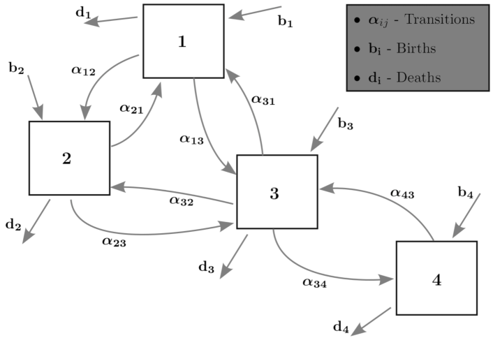
Figure 1: Continuous-time Markov random walk model example. $\alpha_{ij}$ is the transition rate from node $i$ to node $j$ and may be zero, indicating direct migration is impossible without traversing other nodes. $b_{i}$ is the rate at which individuals are introduced into the system at node $i$, and $d_{i}$ is the rate at which individuals in node $i$ are removed from the system.

In an open population model, individuals may enter (birth) or leave (death) the system continuously in time at any node (Figure 1). It is common to model the birth and death rates at node $i$ as being density dependent, with birth rate of $n_{i}b$ and death rate of $n_{i}d$, for constant rates $b$ and $d$ shared across space. Instead, I will allow the birth and death rates to vary spatially, as this will provide a convenient mechanism for accounting for unmodeled spatial variation. To this end, consider birth and death rates that scale with the total population size ($N$). Let $Nb_{i}$ be the rate at which individuals are introduced into node $i$ and let $Nd_{i}$ be the rate at which individuals in node $i$ are removed from the system.

To write a spatio-temporal model for the normalized population process $\mathbf{z}(t)$, it will be helpful to write each of the potential jumps (movement between nodes, births, and deaths) possible in this discrete system. If an individual is introduced at node $i$, then the population at $i$ increases by 1. Notationally, represent this transition in the population process $\mathbf{n}$ as $\mathbf{n}\rightarrow\mathbf{n}+\mathbf{e}_{i}$, where $\mathbf{e}_{i}$ is the canonical vector with $M$ componants, all of which are zero except for the $i$-th element, which is equal to 1. The jump in this birth transition is given by $\mathbf{e}_{i}$. Similarly, a death (removal) at node $i$ decreases the population at node $i$ by 1 and is given by the jump $-\mathbf{e}_{i}$. Spatial movement (transitions) from node $i$ to node $j$, which occur with rate $n_{i}\alpha_{ij}$, have jumps given by $\mathbf{e}_{i}-\mathbf{e}_{j}$. The possible transitions with their rates are given in Table 1.

Table 1: Transitions and Poisson rates in the continuous-time Markov population process.

Description	Transition	Jump	Rate
Birth at node $i$	$\mathbf{n}\rightarrow\mathbf{n}+\mathbf{e}_{i}$	$\mathbf{e}_{i}$	$Nb_{i}$
Death at node $i$	$\mathbf{n}\rightarrow\mathbf{n}-\mathbf{e}_{i}$	$-\mathbf{e}_{i}$	$Nd_{i}$
Move from node $i$ to node $j$	$\mathbf{n}\rightarrow\mathbf{n}+\mathbf{e}_{j}-\mathbf{e}_{i}$	$\mathbf{e}_{j}-\mathbf{e}_{i}$	$n_{i}\alpha_{ij}$

Given an initial unnormalized population state $\mathbf{n}(0)$ at time zero, the transient distribution $\mathbf{n}(t)$ is given by (e.g., Baxendale & Greenwood, 2011)

$$\mathbf{n}(t)=\mathbf{n}(0)+\sum_{ij\neq 0}(\mathbf{e}_{j}-\mathbf{e}_{i})P_{ij}\left[\int_{0}^{t}n_{i}(s)\alpha_{ij}\text{d}s\right]+\sum_{i}\left(\mathbf{e}_{i}P_{0i}\left[\int_{0}^{t}Nb_{i}\text{d}s\right]-\mathbf{e}_{i}P_{i0}\left[\int_{0}^{t}Nd_{i}\text{d}s\right]\right)$$

where

$$P_{ij}(a)\sim Pois(a),\quad i=0,1,\ldots,M;\ j=0,1,\ldots,M;\ i\neq j.$$

The transient distribution for the normalized density $\mathbf{z}=\mathbf{n}/N$ is given by

$$\mathbf{z}(t)=\mathbf{z}(0)+\sum_{ij\neq 0}(\mathbf{e}_{j}-\mathbf{e}_{i})\frac{1}{N}P_{ij}\left[\int_{0}^{t}n_{i}(s)\alpha_{ij}\text{d}s\right]+\sum_{i}\mathbf{e}_{i}\left(\frac{1}{N}P_{0i}\left[Nb_{i}t\right]-\frac{1}{N}P_{i0}\left[Nd_{i}t\right]\right).$$ (6)

Taking the large population limit as $N\rightarrow\infty$ (Kurtz, 1978; Baxendale & Greenwood, 2011) gives the integral equation for the normalized density

$$\mathbf{z}(t)=\mathbf{z}(0)+\sum_{i\neq j}(\mathbf{e}_{j}-\mathbf{e}_{i})\int_{0}^{t}z_{i}(s)\alpha_{ij}\text{d}s+\sum_{i}\mathbf{e}_{i}(b_{i}-d_{i})t.$$ (7)

Details of this calculation are given in Appendix A.

The differential equation associated with (7) is

$$\frac{\partial\mathbf{z}(t)}{\partial t}=\sum_{i\neq j}\alpha_{ij}(\mathbf{e}_{j}-\mathbf{e}_{i})z_{i}(t)+\sum_{i}\mathbf{e}_{i}(b_{i}-d_{i})$$

which has vectorized form

$$\frac{\partial\mathbf{z}(t)}{\partial t}=-\mathbf{Q}^{\prime}\mathbf{z}(t)+(\mathbf{b}-\mathbf{d})$$ (8)

where $\mathbf{b}=[b_{1}\ b_{2}\ \ldots\ b_{M}]^{\prime}$, $\mathbf{d}=[d_{1}\ d_{2}\ \ldots\ d_{M}]^{\prime}$, and $\mathbf{Q}$ is the infinitessimal generator of the CTMC or the Laplacian matrix of the graph

$$\mathbf{Q}=\left(\begin{array}[]{ccccc}\sum_{k}\alpha_{1k}&-\alpha_{12}&-\alpha_{13}&\cdots&-\alpha_{1m}\\ -\alpha_{21}&\sum_{k}\alpha_{2k}&-\alpha_{23}&\cdots&-\alpha_{2m}\\ -\alpha_{31}&-\alpha_{32}&\sum_{k}\alpha_{3k}&\cdots&-\alpha_{3m}\\ \vdots&&&\ddots&\vdots\\ -\alpha_{m1}&-\alpha_{m2}&-\alpha_{m3}&\cdots&\sum_{k}\alpha_{mk}\end{array}\right).$$ (9)

Equation (8) specifies a graph diffusion process where $\mathbf{b}-\mathbf{d}$ is a vector of net inputs and outputs to the system and $-\mathbf{Q}^{\prime}$ is a matrix describing proportional rates of transfer between spatial locations.

3.2 Spatial Models From Random Walks

To specify a spatial model motivated by the differential equation (8), consider modeling the spatial birth and death rates as spatial white noise

$$\boldsymbol{\gamma}=\mathbf{b}-\mathbf{d}\sim N(\mathbf{0},\sigma^{2}\mathbf{I})$$

subject to the constraint that $\mathbf{1}^{\prime}\boldsymbol{\gamma}=0$. This sum-to-zero constraint on $\boldsymbol{\gamma}$ is necessary to ensure the existence of a stationary distribution $\boldsymbol{\pi}$ for (8). The spatio-temporal differential equation (8) can then be written as the RPDE

$$\frac{\partial}{\partial t}\mathbf{z}(t)=-\mathbf{Q}^{\prime}\mathbf{z}(t)+\boldsymbol{\gamma},\quad\boldsymbol{\gamma}\sim N(\mathbf{0},\sigma^{2}\mathbf{I}).$$ (10)

The stationary distribution $\boldsymbol{\pi}$ for the normalized population process $\mathbf{z}$ satisfies the balance equation that $\frac{\partial}{\partial t}\mathbf{z}(t)=\mathbf{0}$, which implies that

$$\mathbf{Q^{\prime}}\boldsymbol{\pi}=\boldsymbol{\gamma},\quad\boldsymbol{\gamma}\sim N(\mathbf{0},\sigma^{2}\mathbf{I})$$

and thus the stationary distribution for (10) is given by

$$\boldsymbol{\pi}\sim N(\mathbf{0},(\mathbf{QQ}^{\prime})^{-}),\text{ with }\mathbf{1}^{\prime}\boldsymbol{\pi}=0.$$ (11)

This stationary distribution is a random field on the discrete spatial support of the population process $\mathbf{z}(t)$ with spatial covariance defined by the spatio-temporal CTMC random walk with infinitessimal generator $\mathbf{Q}$ (9).

3.2.1 Links to Intrinsic Simultaneous Autoregressive Random Fields

The random field in (11) corresponds to an intrinsic simulataneous autoregressive (SAR) model for spatial correlation. This correspondence provides an intuitive approach for specifying the SAR neighborhood structure in situations where some information is known about the spatio-temporal dynamics of the system being modeled.

The standard SAR model can be written (see e.g., Section 4.2.7 of Cressie & Wikle, 2011) as

$$\mathbf{y}\sim N(\mathbf{0},(\mathbf{I}-\mathbf{B})^{-1}\boldsymbol{\Lambda}(\mathbf{I}-\mathbf{B}^{\prime})^{-1})$$

where $\mathbf{B}$ has zeroes on the diagonal and $\boldsymbol{\Lambda}$ is a diagonal matrix with $i$-th diagonal $\Lambda_{ii}$. Then setting

$$B_{ij}=\frac{\alpha_{ji}}{\sum_{k}\alpha_{ik}}\text{ and }\Lambda_{ii}=\frac{1}{\left(\sum_{k}\alpha_{ik}\right)^{2}}$$

expresses (6) as an intrinsic SAR model. As in standard SAR models, the matrix $\mathbf{Q}$ from (4) does not have to be symmetric, but rather can incorporate models for asymmetric random walks. Additionally, if $\mathbf{Q}$ is sparse (many of the $\{\alpha_{ij}\}$ are zero), then sparse matrix methods (e.g., Rue & Held, 2005) can be employed to sample from and evaluate the density in (6).

The SAR models (and related CAR models) have been viewed as unintuitive (Wall, 2004). The spatio-temporal random walk motivation for the spatial model in (11) provides a principled framework for incorporating knowledge about the spatio-temporal spread of a system into a model for spatial autocorrelation.

The random field $\boldsymbol{\pi}$ in (11) is an intrinsic random field, in that only linear combinations are proper (Besag & Kooperberg, 1995). An alternative formulation is that the density for $\boldsymbol{\pi}$ is proper under the constraint that $\boldsymbol{\pi}$ sums to zero over the spatial domain. Intrinsic random fields are often used as prior distributions, where the posterior distribution is proper. For example, consider modeling a Gaussian response $\mathbf{y}$ as

$$\mathbf{y}=\mu\mathbf{1}+\boldsymbol{\pi}+\boldsymbol{\epsilon},\quad\boldsymbol{\epsilon}\sim N(\mathbf{0},\tau^{2}\mathbf{I})$$

where $\boldsymbol{\pi}\sim N(\mathbf{0},(\mathbf{QQ}^{\prime})^{-}),\text{ with }\mathbf{1}^{\prime}\boldsymbol{\pi}=0.$ Under this formulation, $\boldsymbol{\pi}$ is constrained to sum to zero, but $\mu\mathbf{1}+\boldsymbol{\pi}$ is not. This formulation can be seen as a form of restricted spatial regression (Hughes & Haran, 2013; Hanks, Schliep, Hooten & Hoeting, 2015) where the spatial random effect $\boldsymbol{\pi}$ is constrained to be orthogonal to the intercept $\mu\mathbf{1}$.

3.2.2 Identifiability

The likelihood of (11)

$$f(\boldsymbol{\pi}|\mathbf{Q})\propto|\mathbf{QQ}^{\prime}|^{-1/2}\exp\left\{-\frac{1}{2}\boldsymbol{\pi}^{\prime}\mathbf{QQ}^{\prime}\boldsymbol{\pi}\right\}$$

is a function of $\mathbf{QQ}^{\prime}$, rather than purely a function of the infinitessimal generator $\mathbf{Q}$. Thus, if there are two generator matrices $\mathbf{Q}$ and $\mathbf{W}$ such that $\mathbf{QQ}^{\prime}=\mathbf{WW}^{\prime}$, then $\mathbf{Q}$ is not identifiable. However, the special structure required for a generator matrix of a CTMC allows us to prove that $\mathbf{Q}$ is identifiable in all but pathological situations.

Theorem 3.1

If $\mathbf{Q}$ and $\mathbf{W}$ are both generator matrices (9) for irreducible $M$-state CTMCs, and at least one row of $\mathbf{Q}$ has more than one nonzero off-diagonal entry, then $\mathbf{QQ}^{\prime}$=$\mathbf{WW}^{\prime}$ if and only if $\mathbf{Q}=\mathbf{W}$.

The proof is given in Appendix B. The significance of this result is that the only forms for $\mathbf{Q}$ that are unidentifiable come when the embedded chain of the irreducible CTMC governed by $\mathbf{Q}$ is deterministic and topologically the graph given by $\mathbf{Q}$ is a loop, with flow only possible in one direction (either clockwise or counter-clockwise). In all other graph topologies, identifiability is guaranteed.

4 Example 1: Random walk models for spatial genetic variation on stream networks

I now present two examples of spatial analyses using the assumption of a spatio-temporal random walk generating process leading to a spatial random effect. The first example comes from landscape ecology, where a common goal is to understand how the landscape influences spatial connectivity or correlation. Random walk models are among the most common models for gene flow, both in theory and in practice. McRae (2006) showed that under a random walk model for migration, a common formulation of genetic dissimilarity (the linearized fixation index) was proportional to the circuit resistance distance (Klein & Randić, 1993) between the nodes in question. Under the formulation of McRae (2006), the spatial domain is envisioned as a graph of spatial nodes with symmetric edge weights $\alpha_{ij}$ proportional to the (symmetric) rate of random walkers between nodes. The resistance distance is the effective resistance in an electric circuit where the nodes are connected by resistors with resistance $1/\alpha_{ij}$ equal to the inverse of the migration rate. This approach to studying gene flow is known as the isolation by resistance approach, and is often used to explore the relationship between landscape features and gene flow.

While most studies addressing isolation by resistance choose between a finite number of pre-specified edge weights (resistances), Hanks & Hooten (2013) modeled the observed pairwise genetic distance matrix using the generalized Wishart distribution of McCullagh (2009) with symmetric precision matrix $\mathbf{Q}$ (9) and made inference on the edge weights $\alpha_{ij}$ as a function of landscape covariates. Instead of using the RPDE stationary distribution approach that gives rise to (11), Hanks & Hooten (2013) considered a variogram argument, as follows. Using links between symmetric random walks and electric circuits (Doyle & Snell, 1984), McRae (2006) showed that under a random walk model for migration, a common formulation of genetic dissimilarity (the linearized fixation index) was proportional to the resistance distance (Klein & Randić, 1993). Hanks & Hooten (2013) showed that the resistance distance was exactly the variogram (expected squared difference) of an intrinsic Gaussian spatial random field with precision matrix $\mathbf{Q}$. While this provides an interesting link between random walks and variograms, our goal in this analysis is to directly motivate a spatial model by the stationary distribution of a spatio-temporal model, something not explicitly considered by Hanks & Hooten (2013).

The isolation by resistance approach assumes symmetric edge weights (and thus symmetric migration rates), though often it would be more realistic to assume asymmetric migration rates reflecting source and sink dynamics. As an example, consider the system studied by Kanno et al. (2011), consisting of trout in the Jefferson-Hill Spruce Brook in Connecticut, USA. 470 trout were captured at 173 spatial locations along the brook (Figure 2) and genotyped, with microsatellite allele data obtained at 15 loci. An isolation by resistance approach would require symmetric migration rates between upstream and downstream locations, but a more realistic model (which I will propose) would consider asymmetric migration rates reflecting the potentially increased difficulty in moving upstream relative to moving downstream.

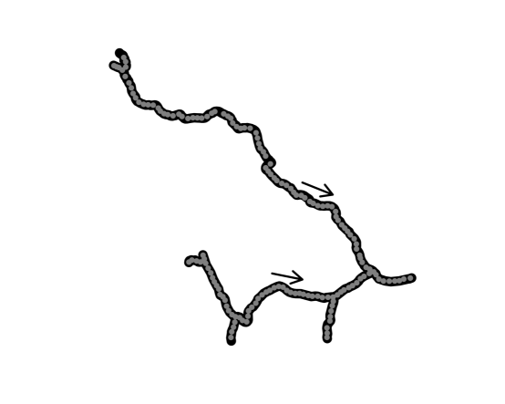
Figure 2: Trout sampling locations on the Jefferson Hill Spruce Brook.

Additionally, Kanno et al. (2011) examine the effect of two seasonal blockages of the brook - two locations where the brook dries up and is seasonally impassible to the trout. The hypothesized drivers of gene flow and genetic connectivity among the trout population on Jefferson Hill Spruce Brook are both directional (differential rates of movement upstream and downstream) and non-directional (decreased connectivity between stream locations on opposite sides of the seasonal blockages). If spatio-temporal trout movement data were available, modeling these directional and non-directional responses to covariates would be straightforward (Hooten et al., 2010; Hanks, Hooten & Alldredge, 2015). For example, movement could be envisioned as occuring on a graph with a node at each spatial location where trout were sampled, and edge weights equal to random walk transition rates between nodes could be modeled as

$$\alpha_{ij}=\begin{cases}\frac{1}{d_{ij}}\text{exp}\left\{\beta_{0}+\beta_{1}u_{ij}+\beta_{2}v_{ij}\right\}&\text{if nodes }i\text{ and }j\text{ are neighbors}\\ 0&\text{otherwise}\end{cases}$$ (12)

where $\{u_{ij}\}$ and $\{v_{ij}\}$ are indicator variables with $u_{ij}=1$ if node $j$ is downstream from node $i$ and $v_{ij}=1$ if a seasonal blockage is located between nodes $i$ and $j$. In this formulation, each node on a branch of the stream network has two neighbors, one upstream and one downstream, and edge weights $\alpha_{ij}$ are zero for all other non-neighboring nodes. Each node at a confluence of two stream branches will have three neighbors, one downstream and two upstream. The rate at which a random walker at a node $i$ on a branch of the stream network transitions to the nearest upstream node $j$ is $\alpha_{ij}=1/d_{ij}\text{exp}\{\beta_{0}\}$ if there is not a seasonal blockage between nodes $i$ and $j$. Similarly, the rate at which the random walker transitions from $i$ to the nearest downstream node $k$ is $\alpha_{ik}=1/d_{ik}\text{exp}\{\beta_{0}+\beta_{1}\}$. The parameter $\beta_{2}$ models the additive effect that a seasonal blockage has on log-transition rates. Together, this simple random walk model allows for transition rates that vary with direction and location based on known spatial stream characteristics.

A spatial model for the observed microsatellite allele data could then be specified with a latent spatial autocorrelation modeled using the stationary distribution (11) of the random walk model (12) when driven by time-homogeneous white Gaussian noise, as described in Section 3.2.

Microsatellite allele data were observed at $L=15$ distinct loci for each spatially referenced trout captured. At the $\ell^{\text{th}}$ locus, $\ell=1,2,\ldots,L$, denote the list of all distinct observed alleles from all individuals in the study as $\{a_{\ell 1},a_{\ell 2},\ldots,a_{\ell K_{\ell}}\}$. Following Guillot et al. (2005) and others, I model the two observed alleles for each (diploid) individual as arising from a multinomial distribution with spatially varying allele probabilities $\mathbf{p}_{s\ell}=(p_{s\ell 1}\ p_{s\ell 2}\ \ldots\ p_{s\ell K_{\ell}})^{\prime}$, where $s\in\{1,2,\ldots,S\}$ indexes the spatial location.

Let $y_{sip\ell k}=1$ if the $p^{\text{th}}$ (indexing ploidy) observed allele at the $\ell^{\text{th}}$ locus is $a_{\ell k}$ for the $i^{\text{th}}$ individual at the $s^{\text{th}}$ spatial location, and $y_{sip\ell k}=0$ otherwise. Then the multinomial probit model (e.g., Albert & Chib, 1993) for categorical data is often specified in terms of latent variables, $\mathbf{z}$, as follows. Let

$$y_{sip\ell k}=\begin{cases}1&\ ,\ z_{sip\ell k}=\max\{z_{sip\ell a},\ a=1,\ldots,K_{\ell}\}\\ 0&\ ,\ \text{otherwise}\end{cases}$$ (13)

where

$$z_{sip\ell k}\sim N(\mu_{\ell k}+\eta_{s\ell k},1).$$ (14)

Then the allele $a_{\ell k}$ makes up a fraction $p_{s\ell k}$ of the genetic makeup of the subpopulation at location $s$, where

$$p_{s\ell k}=\text{Prob}\left(z_{sip\ell k}=\max\{z_{sip\ell a},\ a=1,\ldots,K_{\ell}\}\right)$$

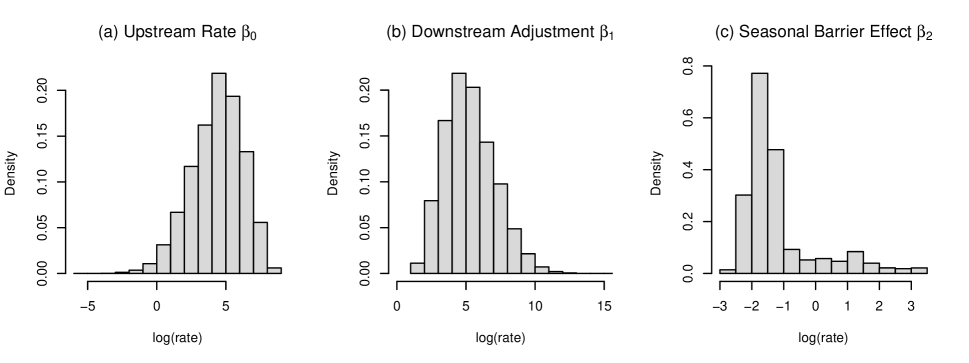
Figure 3: Posterior histograms of random walk model parameters in the spatial genetic analysis of trout in the JeffersonHill Spruce Brook.

The mean of the latent variable $z_{sip\ell k}$ in (14) consists of the sum of two effects. The first is $\mu_{\ell k}$, an allele specific intercept which determines the relative frequency of the $k^{\text{th}}$ allele at the $\ell^{\text{th}}$ locus across the entire population being studied. Large values of $\mu_{\ell k}$, relative to $\mu_{\ell k^{\prime}}$ make it more likely that $z_{sip\ell k}$ will be larger than $z_{sip\ell k^{\prime}}$, and so the $k^{\text{th}}$ allele will be more prevalent than the $(k^{\prime})^{\text{th}}$ allele. Note that the model (13)-(14) is invariant to a shift in all $\mu_{\ell k}$, as the likelihood is a function of the contrasts $z_{sip\ell k}-z_{sip\ell k^{\prime}}$, and not the actual values of $z_{sip\ell k}$. Thus, if $\mu_{\ell k}$ were replaced by $\mu_{\ell k}+c$ for $k=1,2,\ldots,K_{\ell}$ and some constant $c$, the likelihood of the observed allele data would remain unchanged. To maintain model identifiability, fix $\mu_{\ell 1}=0$ for $\ell=1,2,\ldots,L$, as only the relative differences (contrasts) in $\mu_{\ell k}$ are identifiable.

The second term in the mean of (14) is $\eta_{s\ell k}$, which is a spatially varying random effect that allows the allele frequencies $\mathbf{p}_{s\ell}$ to vary over the stream network. Following the reasoning in Section 3.2, the spatial random effects are modeled as the stationary distribution of a random walk process driven by time-homogeneous noise. Let

$$\boldsymbol{\eta}_{\ell k}=\left[\begin{array}[]{c}\eta_{1\ell k}\\ \eta_{2\ell k}\\ \vdots\\ \eta_{n\ell k}\end{array}\right]\sim N(\mathbf{0},(\mathbf{QQ}^{\prime})^{-1}),\quad\mathbf{1}^{\prime}\boldsymbol{\eta}_{\ell k}=0$$ (15)

where $\mathbf{Q}$ is the infinitessimal generator (9) of the random walk with transition rates (12).

The model is completed by specifying diffuse Gaussian priors for the random walk parameters $\beta_{0},\ \beta_{1},\ \beta_{2}$ and the allele specific intercepts

$$\beta_{j}\sim N(0,10^{2}),\quad j=0,1,2$$ (16)

$$\mu_{\ell k}\sim N(0,10^{2}),\quad\ell=1,2,\ldots,L;\quad k=2,3,\ldots,K_{\ell}.$$ (17)

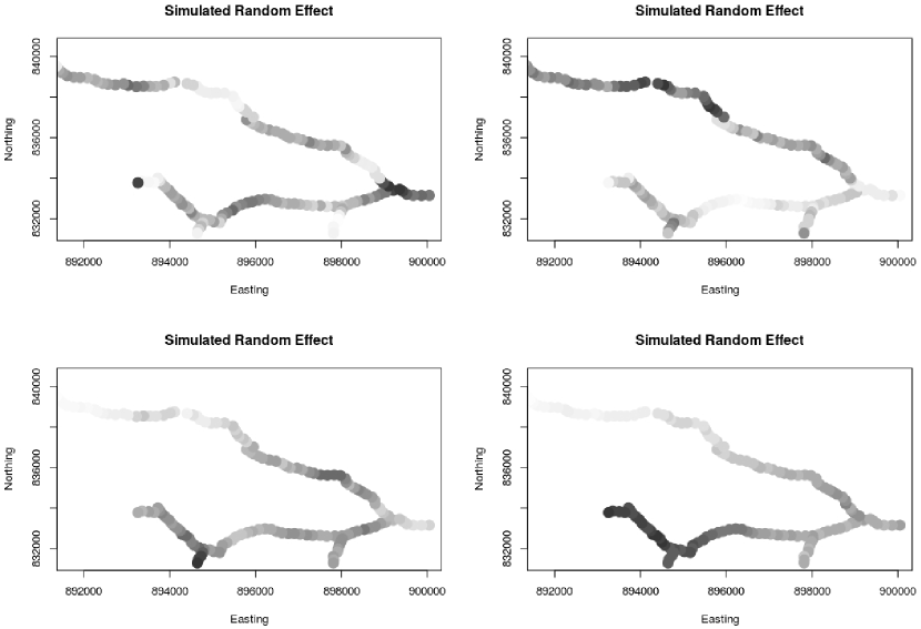
Figure 4: Four realizations of random fields on the Jefferson-Hill Spruce Brook simulated using posterior mean parameter values of the random walk covariance model.

A Markov chain Monte-Carlo (MCMC) algorithm was constructed to sample from the posterior distribution of model parameters, given the observed microsatellite allele data. Fifteen chains were run with different starting values. Each chain was run for $10^{6}$ iterations, with the first $10^{5}$ samples discarded as burn in. Convergence was assessed by comparing posterior histograms obtained from only the first half of each chain with posterior histograms obtained from only the second half of each chain. Histograms of the marginal posterior distributions of the random walk parameters are given in Figure 3. The posterior distribution for $\beta_{1}$ is greater than zero, indicating that the data support the anisotropic hypothesis that gene flow is more rapid downstream than upstream. The posterior distribution for $\beta_{2}$, which captures the effect of the seasonal blockages, overlaps zero (Figure 3(c)), with the $95\%$ equal-tailed credible interval being bounded by $(-2.4,2.2)$. This indicates only weak support (if any) for the hypothesis that the seasonal blockages affect gene flow.

Posterior distributions for the allele specific intercepts are not shown, and posterior mean values for the intercepts ranged from $-2.2$ to $0.7$. To qualitatively illustrate the genetic correlation structure implied by the estimated parameters, four realizations of random fields on the stream network were simulated using the posterior mean parameter values. These random fields are shown in Figure 4. The constructive spatio-temporal approach proposed here provides a valid autoregressive spatial model for data collected on a stream network. In contrast, VerHoef2010 present a moving average (convolution) approach to modeling spatial autocorrelation on stream networks.

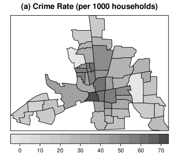
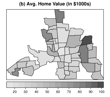
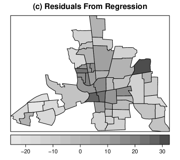
Figure 5: Observed 1980 crime rates (a) and average home values (b) in 49 neighborhoods in Columbus, Ohio, USA. The residuals (c) from a simple linear regression of crime rates on average home values show clear autocorrelation. A standard spatial analysis might include a spatial random effect with SAR neighborhood structure (d) to account for the spatial autocorrelation in the data. We contrast this with a graph diffusion based approach to jointly modeling spatial autocorrelation and the effect of the spatial covariate (average home values).

5 Example 2: Crime rates in Columbus, OH.

A second example illustrates how considering a spatio-temporal generating process can provide insights into modeling the interplay between mean and covariance structure in spatial models. As mentioned previously, recent recognition of the potential for spatial confounding (e.g., Hughes & Haran, 2013; Hanks, Schliep, Hooten & Hoeting, 2015) suggests that correctly modeling the relationship between the fixed and random effects in a model is important, even if we only desire to interpret the relationship between fixed effects and the response.

Consider the case of 1980 crime rates in 49 neighborhoods in Columbus, Ohio, USA (Anselin, 1988). Figure 5(a) shows the number of residential burglaries and vehicle thefts per thousand housholds in each of the 49 neighborhoods. Figure 5(b) shows the average value of homes in each neighborhood, in thousands of dollars. These data are freely available in the ‘spdep’ package (Bivand & Piras, 2015) of the R statistical computing environment (R Core Team, 2015).

A preliminary linear regression with crime rates as response and average home values as predictor variable indicates a negative correlation between average home values and crime rates. However, the residuals from this simple linear regression are shown in Figure 5(c) and show clear spatial autocorrelation. A standard spatial analysis might consider the following spatial linear model

$$\mathbf{c}=\mu\mathbf{1}+\beta\mathbf{h}+\sigma\boldsymbol{\eta}+\boldsymbol{\epsilon},\quad\boldsymbol{\epsilon}\sim N(\mathbf{0},\tau^{2}\mathbf{I})$$ (18)

$$\boldsymbol{\eta}\sim N(\mathbf{0},(\mathbf{QQ}^{\prime})^{-1})\text{ with }\mathbf{1}\boldsymbol{\eta}=0$$ (19)

where $\mathbf{c}$ is a vector of the 1980 crime rates, $\mathbf{h}$ is a vector of average home values, $\boldsymbol{\eta}$ is a spatial random effect with SAR structure defined by $\mathbf{Q}$, and $\boldsymbol{\epsilon}$ is nonspatial error. A symmetric neighborhood graph was defined with edges between all polygons that share a polygon edge, as shown in Figure 5(d). If neighborhoods $i$ and $j$ are neighbors, say that $i\sim j$ or, equivalently in this symmetric relationship, $j\sim i$. The matrix $\mathbf{Q}$ in (19) then has elements

$$Q_{ij}=\begin{cases}-1&\ ,\text{ if }i\neq j,\ i\sim j\\ 0&\ ,\text{ if }i\neq j,\ i\nsim j\\ \sum_{j\sim i}1&\ ,\text{ if }i=j\end{cases}.$$

Thus $\boldsymbol{\eta}$ is an intrinsic spatial random effect with precision matrix $\mathbf{Q}^{2}$. Heuristically, $\boldsymbol{\eta}$ is a missing covariate that is spatially smooth on the support of the 49 neighborhoods in Columbus.

Now contrast this purely spatial approach with an approach based on considering a spatio-temporal graph diffusion generating process. As noted in Section 3.1, the differential equation (8) resulting from the large $N$ limit of the population-level random walk process is a diffusion process defined by a vector of inputs to the system and a matrix $-\mathbf{Q}^{\prime}$ encoding rates of transfer between spatial nodes in the graph. In this spirit, consider a process where the inputs (sources and sinks) are random variables with mean defined by the predictor variable (average home value) and spatial diffusion rates defined by the spatial neighborhood graph. Note that while this is not a science-based mechanistic model for crime in Columbus, it does provide two competing models for how crime rates are related to average home values. In the standard spatial model, the spatial random effect $\boldsymbol{\eta}$ is a missing covariate unrelated to average home values $\mathbf{h}$. In the graph diffusion based model presented below, a diffusion process spatially smooths the effect of $\mathbf{h}$, similar to a moving average (or convolution-based) spatial model (e.g., Lee et al., 2005).

As an alternative to the standard spatial mixed effect model in (18)-(19), consider modeling crime rates ($\mathbf{c}$) as

$$\mathbf{c}=\mu\mathbf{1}+\boldsymbol{\pi}+\boldsymbol{\epsilon}$$ (20)

where $\boldsymbol{\pi}$ is the stationary distribution of the spatio-temporal graph diffusion process $\mathbf{z}(t)$ defined elementwise as

$$\frac{\partial z_{i}(t)}{\partial t}=-\kappa n_{i}z_{i}(t)+\sum_{j\sim i}\kappa z_{j}(t)+\beta\cdot h_{i}+\delta_{i}.$$ (21)

The first term on the right hand side of (21) defines the flow out of node $i$ to the $n_{i}=\sum_{j\sim i}1$ neighboring nodes. The second term defines the flow into node $i$ from other nodes. The net input/output from “births” and “deaths” into node $i$ is $\beta h_{i}+\delta_{i}$. The intuition here is that the spatial source of crime in Columbus neighborhoods is correlated with home values, and that crime spreads spatially out from neighborhoods with high crime rates to neighboring regions, with a constant diffusion rate of $\kappa$ between all neighboring nodes.

If $\delta_{i}$ are modeled as independent zero mean Gaussian random variables, the RPDE can be written in vector form as

$$\frac{\partial\mathbf{z}(t)}{\partial t}=-\kappa\mathbf{Q}^{\prime}\mathbf{z}(t)+\beta\mathbf{h}+\boldsymbol{\delta},\quad\boldsymbol{\delta}\sim N(\mathbf{0},\sigma^{2}\mathbf{I})$$ (22)

and the stationary distribution $\boldsymbol{\pi}$ satisfies

$$\kappa\mathbf{Q}^{\prime}\boldsymbol{\pi}=\beta\mathbf{h}+\boldsymbol{\delta},$$

or, equivalently

$$\boldsymbol{\pi}\sim N\left(\frac{\beta}{\kappa}(\mathbf{Q}^{\prime})^{-1}\mathbf{h},\frac{\sigma^{2}}{\kappa}(\mathbf{QQ}^{\prime})^{-1}\right),\quad\mathbf{1}^{\prime}\boldsymbol{\pi}=0$$

where $(\mathbf{Q}^{\prime})^{-1}$ is the Bott-Duffin constrained generalized inverse (Bott & Duffin, 1953) of $\mathbf{Q}^{\prime}$. The data model (20) for the graph diffusion spatial model can then be written as

$$\mathbf{c}=\mu\mathbf{1}+\tilde{\beta}(\mathbf{Q}^{\prime})^{-1}\mathbf{h}+\tilde{\sigma}\boldsymbol{\eta}+\boldsymbol{\epsilon}$$ (23)

with $\tilde{\beta}=\beta/\kappa$, $\tilde{\sigma}=\sigma/\kappa$, and $\boldsymbol{\eta}$ a random effect defined as in (19). Without strong prior information, $\kappa$ will be unidentifiable. Instead, consider inference on $\tilde{\beta}=\beta/\kappa$ and $\tilde{\sigma}=\sigma/\kappa$, which are identifiable. In this formulation, the only difference between the standard spatial model in (18) and the graph diffusion based spatial model in (23) is that the fixed effect $\mathbf{h}$ in (18) is smoothed by $(\mathbf{Q}^{\prime})^{-1}$ in (23).

Within a Bayesian framework for inference, I assigned flat Gaussian priors to the regression parameters $\mu$, $\beta$, and $\tilde{\beta}$. Flat half-normal priors were chosen for the spatial random effect variance parameters $\sigma$ and $\tilde{\sigma}$, and an inverse-gamma prior was chosen for the non-spatial error variance $\tau^{2}$. Inference on the parameters in (19) and (23) was obtained by a Markov chain Monte Carlo sampler. In each case, the MCMC sampler was run for $10^{5}$ iterations. Convergence was assessed by comparing histograms of samples from the first half of the Markov chain with histograms of samples from the second half of the Markov chain.

Table 2: Posterior results for parameters in the spatial and graph-diffusion based models for crime in Columbus, OH neighborhoods. The graph diffusion model fits the data better as measured by DIC.

Parameter	Post. Mean	Post. 0.025 Quantile	Post. 0.975 Quantile
Spatial Model (18)     DIC = 442.10
$\mu$	35.12	32.09	38.12
$\beta$	-9.28	-12.48	-6.16
$\sigma$	1.81	0.31	3.50
$\tau$	10.75	8.86	13.04
Graph Diffusion Model (23)     DIC = 411.52
$\mu$	35.13	31.89	38.33
$\tilde{\beta}$	-9.38	-12.89	-5.92
$\tilde{\sigma}$	0.94	0.03	2.67
$\tau$	11.51	9.68	13.75

Posterior means and 95$\%$ credible interval bounds are shown in Table 2. To compare models, I computed the Deviance information criterion (DIC, Spiegelhalter et al., 2002). Posterior distributions for $\mu$ and $\beta$ from the spatial model (18) are similar to those of $\mu$ and $\tilde{\beta}$ from the graph diffusion model (23); however, the standard deviation $\sigma$ of the spatial random effect $\boldsymbol{\eta}$ in the spatial model (18) is larger than the corresponding standard deviation $\tilde{\sigma}$ in the graph diffusion model (23). This indicates that the need for the spatial random effect is greater in the spatial model than in the graph diffusion model where the home value covariate was smoothed by $(\textbf{Q}^{\prime})^{-1}$. The DIC of the graph diffusion model (DIC=411) was lower than that of the standard spatial model (DIC=442), indicating that in this case, considering a spatio-temporal generating process resulted in a better model fit than would be obtained by the inclusion of a standard spatial random effect.

6 Discussion

While we have focused on discrete space models, this general approach has potential for application in continuous space as well. Spatial deformation approaches to nonstationary covariance (e.g., Schmidt & O’Hagan, 2003; Lindgren et al., 2011) can be viewed as stationary distributions of diffusion processes with spatially heterogeneous diffusion rates. Reaction-diffusion models are common in ecology and other fields (e.g., Keeling et al., 2004; Hu et al., 2013) and would provide a natural spatio-temporal generating process basis for spatial random effect models in a wide variety of systems. Finite element basis and grid-based approaches to approximating continuous spatial fields have a long history in spatio-temporal (e.g., Wikle & Hooten, 2010) and spatial (e.g., Lindgren et al., 2011) analysis, and could be used to approximate the stationary distribution of a continuous (infinite-dimensional) spatio-temporal generating process with a finite number of basis functions.

Current standard approaches to modeling spatial correlation focus on nonparametric random effect models. This work proposes a parametric constructive approach to modeling spatial random effects based on an assumed spatio-temporal generating process. The two examples give some indication of how this approach may be used. In the first example, existing scientific knowledge about the system (gene flow on a stream network) was used to specify a spatio-temporal generating model (a population-level random walk), and the stationary distribution of this spatio-temporal process defined the distribution of the spatial random effect used to model genetic correlation. In the second example, a descriptive approach was taken to compare multiple models for spatial variation. In particular, for the Columbus crime data, the graph diffusion model provided a better model fit than was obtained using a standard spatial random effect model. Modeling spatial random effects nonparametrically is the current standard practice; however, there are benefits to parametric modeling of spatial random effects when the existing science can suggest a spatio-temporal generating mechanism.

Appendix A: Large population limits of population processes

The interested reader is referred to Kurtz (1981) for a full treatment of stochastic population processes. This derivation follows the spirit of Kurtz (1981) and Baxendale & Greenwood (2011), but with the novelty of birth and death rates that are not density dependent.

Following from (6) in Section 3.1, the transient distribution for the normalized density $\mathbf{z}=\mathbf{n}/N$ is given by

$$\mathbf{z}(t)=\mathbf{z}(0)+\sum_{ij\neq 0}(\mathbf{e}_{j}-\mathbf{e}_{i})\frac{1}{N}P_{ij}\left[\int_{0}^{t}n_{i}(s)\alpha_{ij}\text{d}s\right]+\sum_{i}\mathbf{e}_{i}\left(\frac{1}{N}P_{0i}\left[Nb_{i}t\right]-\frac{1}{N}P_{i0}\left[Nd_{i}t\right]\right)$$

where

$$P_{ij}(a)\sim Pois(a),\quad i=0,1,\ldots,M;\ j=0,1,\ldots,M;\ i\neq j.$$

Note that

$$P_{ij}(a) =a+(P_{ij}(a)-a)$$

$$=a+W_{ij}(a)\ ,\quad\quad W_{ij}(a)\sim(0,a)$$

where each $W_{ij}$ has mean zero on constant variance. Applying this to the transient distribution gives

$$\mathbf{z}(t) =\mathbf{z}(0)+\sum_{ij\neq 0}(\mathbf{e}_{j}-\mathbf{e}_{i})\frac{1}{N}\left[\int_{0}^{t}n_{i}(s)\alpha_{ij}\text{d}s\right]+\sum_{i}\mathbf{e}_{i}\left(b_{i}t-d_{i}t\right)$$

$$+\frac{1}{N}\left(\sum_{i\neq j}(\mathbf{e}_{j}-\mathbf{e}_{i})W_{ij}\left[\int_{0}^{t}n_{i}(s)\alpha_{ij}\text{d}s\right]+\sum_{i}\mathbf{e}_{i}\left(W_{0i}\left[Nb_{i}t\right]-W_{i0}\left[Nd_{i}t\right]\right)\right).$$

Consider a fixed $t>0$ and note that $N\geq n_{i}(s)$ for all $s\in(0,t)$. This gives the result that

$$\int_{0}^{t}n_{i}(s)\alpha_{ij}\text{d}s\leq N\alpha_{ij}t.$$

Then to show that all terms above including random variables $W_{ij}$ disappear in the limit as $N\rightarrow\infty$, it is enough to consider the behavior of

$$\frac{1}{N}W(Na),\quad W(a)\sim(0,a)$$

for a constant $a>0$. It is trivial to note that

$$E\left[\frac{1}{N}W(Na)\right]=0$$

and that

$$Var\left[\frac{1}{N}W(Na)\right]=\frac{1}{N^{2}}Na$$

which vanishes in the limit as $N\rightarrow\infty$.

Then, in the large population limit, the transient distribution of the normalized population $\mathbf{z}(t)$ will be given by

$$\mathbf{z}(t)=\mathbf{z}(0)+\sum_{i\neq j}(\mathbf{e}_{j}-\mathbf{e}_{i})\frac{1}{N}\left[\int_{0}^{t}n_{i}(s)\alpha_{ij}\text{d}s\right]+\sum_{i}\mathbf{e}_{i}\left(b_{i}t-d_{i}t\right).$$

Appendix B: Proof of Theorem 3.1

In this appendix, we prove Theorem 3.1. The proof follows from the fact that $\mathbf{QQ}^{\prime}$ is a Gramian matrix (e.g., GentleText) and thus $\mathbf{QQ}^{\prime}=\mathbf{WW}^{\prime}$ if and only if $\mathbf{W}=\mathbf{QU}^{\prime}$ for a real unitary matrix $\mathbf{U}^{\prime}$. As $\mathbf{W}$ and $\mathbf{Q}$ are both generators for CTMC random walks, their rows sum to zero ($\mathbf{Q1}=\mathbf{W1}=\mathbf{0}$), with negative diagonal entries ($q_{ii}<0$, $w_{ii}<0$) and non-negative off-diagonal entries ($q_{ij}\geq 0$, $w_{ij}\geq 0$ for $i\neq j$). If $\mathbf{Q}$ and $\mathbf{W}$ are both generators for irredicible CTMCs, then both matrices have rank $n-1$ and their null spaces are both spanned by the $\mathbf{1}$ vector. As $\mathbf{W1}=\mathbf{0}$, it follows that $\mathbf{QU}^{\prime}\mathbf{1}=\mathbf{0}$ and thus $\mathbf{U}^{\prime}\mathbf{1}=\lambda\mathbf{1}$ for some $\lambda$. The eigenvalues of any unitary matrix $\mathbf{U}^{\prime}$ have absolute value equal to 1, so $\lambda$ either equals $1$ or $-1$. If $\mathbf{u}^{\prime}_{i}$ is the $i$-th row of $\mathbf{U}^{\prime}$, then $\mathbf{u}^{\prime}_{i}\mathbf{1}$ equals either 1 or $-1$, but since $\mathbf{U}$ is unitary, $\mathbf{u}^{\prime}_{i}\mathbf{u}_{i}=1$. These requirements both hold if and only if $\mathbf{u}_{i}=\lambda\mathbf{e}_{k}$, where $\mathbf{e}_{k}$ is the canonical vector with $k$-th element equal to 1 and all other elements equal to zero. As $\mathbf{U}$ is of full rank, the rows of $\mathbf{U}^{\prime}$ must contain a full set of canonical vectors spanning $\mathcal{R}^{n}$.

First consider the case where $\lambda=1$. Then $\mathbf{U}^{\prime}$ is a permutation matrix, with the columns of $\mathbf{W}$ being permuted columns of $\mathbf{Q}$. However, as $\mathbf{W}$ and $\mathbf{Q}$ are generator matrices, each diagonal entry of $\mathbf{W}$ and $\mathbf{Q}$ must be negative, while all off-diagonal entries are non-negative. This can only hold for $\mathbf{W}$ if the permutation matrix $\mathbf{U}^{\prime}$ is the identity matrix, and thus $\mathbf{W}=\mathbf{Q}$.

Now consider the case where $\lambda=-1$. Again $\mathbf{U}^{\prime}$ permutes the columns of $\mathbf{Q}$, but now the sign of all entries is changed through multiplication by $\lambda=-1$. So $w_{ii}=-q_{ik}$ and $w_{ik}=-q_{ii}$ for some $k$. As $\mathbf{W}$ is a generator matrix, $w_{ii}=-\sum_{j\neq i}w_{ij}$, which is only possible if $q_{ik}$ is the only non-zero off-diagonal entry in the $i$-th row of $\mathbf{Q}$. This completes the proof.

References

- (1)
-
Albert & Chib (1993)
Albert, J. & Chib, S. (1993),
‘Bayesian analysis of binary and polychotomous response data’, Journal
of the American Statistical Association 88(422), 669–679.
http://www.jstor.org/stable/2290350 - Anselin (1988) Anselin, L. (1988), Spatial econometrics: methods and models, Vol. 4, Springer Science & Business Media.
- Assunção & Krainski (2009) Assunção, R. & Krainski, E. (2009), ‘Neighborhood dependence in bayesian spatial models’, Biometrical Journal 51(5), 851–869.
- Baxendale & Greenwood (2011) Baxendale, P. H. & Greenwood, P. E. (2011), ‘Sustained oscillations for density dependent markov processes’, Journal of mathematical biology 63(3), 433–457.
- Besag (1974) Besag, J. (1974), ‘Spatial interaction and the statistical analysis of lattice systems’, Journal of the Royal Statistical Society. Series B (Methodological) 36(2), 192–236.
- Besag & Kooperberg (1995) Besag, J. & Kooperberg, C. (1995), ‘On conditional and intrinsic autoregressions’, Biometrika 82(4), 733.
-
Bivand & Piras (2015)
Bivand, R. & Piras, G. (2015),
‘Comparing implementations of estimation methods for spatial econometrics’,
Journal of Statistical Software 63(18), 1–36.
http://www.jstatsoft.org/v63/i18 - Bott & Duffin (1953) Bott, R. & Duffin, R. (1953), ‘On the algebra of networks’, Transactions of the American Mathematical Society 74(1), 99–109.
- Cressie (1993) Cressie, N. (1993), Statistics for Spatial Data, Wiley-Interscience.
- Cressie & Wikle (2011) Cressie, N. & Wikle, C. (2011), Statistics for spatio-temporal data, Vol. 465, Wiley.
- Diggle & Ribeiro (2007) Diggle, P. & Ribeiro, P. J. (2007), Model-based geostatistics, Springer.
- Doyle & Snell (1984) Doyle, P. & Snell, J. (1984), ‘Random walks and electric networks’.
-
Guillot et al. (2005)
Guillot, G., Estoup, A., Mortier, F. & Cosson, J. F.
(2005), ‘A spatial statistical model for
landscape genetics.’, Genetics 170(3), 1261–1280.
http://www.ncbi.nlm.nih.gov/pubmed/15520263 - Hanks & Hooten (2013) Hanks, E. M. & Hooten, M. B. (2013), ‘Circuit theory and model-based inference for landscape connectivity’, Journal of the American Statistical Association 108, 22–33.
- Hanks, Hooten & Alldredge (2015) Hanks, E. M., Hooten, M. B. & Alldredge, M. W. (2015), ‘Continuous-time discrete-space models for animal movement’, The Annals of Applied Statistics 9(1), 145–165.
- Hanks, Schliep, Hooten & Hoeting (2015) Hanks, E. M., Schliep, E. M., Hooten, M. B. & Hoeting, J. A. (2015), ‘Restricted spatial regression in practice: geostatistical models, confounding, and robustness under model misspecification’, Environmetrics 26(4), 243–254.
- Hodges & Reich (2010) Hodges, J. S. & Reich, B. J. (2010), ‘Adding spatially-correlated errors can mess up the fixed effect you love’, The American Statistician 64(4), 325–334.
-
Hooten et al. (2010)
Hooten, M. B., Johnson, D. S., Hanks, E. M. & Lowry, J. H.
(2010), ‘Agent-based inference for animal
movement and selection’, Journal of Agricultural, Biological, and
Environmental Statistics 15(4), 523–538.
http://www.springerlink.com/index/10.1007/s13253-010-0038-2 - Hu et al. (2013) Hu, J., Kang, H.-W. & Othmer, H. G. (2013), ‘Stochastic analysis of reaction-diffusion processes’, Bulletin of Mathematical Biology .
- Hughes & Haran (2013) Hughes, J. & Haran, M. (2013), ‘Dimension reduction and alleviation of confounding for spatial generalized linear mixed models’, Journal of the Royal Statistical Society: Series B (Statistical Methodology) 75(1), 139–159.
- Kanno et al. (2011) Kanno, Y., Vokoun, J. C. & Letcher, B. H. (2011), ‘Fine-scale population structure and riverscape genetics of brook trout (salvelinus fontinalis) distributed continuously along headwater channel networks’, Molecular Ecology 20(18), 3711–3729.
-
Keeling et al. (2004)
Keeling, M. J., Brooks, S. P. & Gilligan, C. a. (2004), ‘Using conservation of pattern to estimate spatial
parameters from a single snapshot.’, Proceedings of the National
Academy of Sciences of the United States of America 101(24), 9155–60.
http://www.pubmedcentral.nih.gov/articlerender.fcgi?artid=428489&tool=pmcentrez&rendertype=abstract - Klein & Randić (1993) Klein, D. & Randić, M. (1993), ‘Resistance distance’, Journal of Mathematical Chemistry 12(1), 81–95.
- Kloeden & Platen (1992) Kloeden, P. E. & Platen, E. (1992), Numerical solution of stochastic differential equations, Vol. 23, Springer Science & Business Media.
- Kurtz (1978) Kurtz, T. G. (1978), ‘Strong approximation theorems for density dependent markov chains’, Stochastic Processes and Their Applications 6(3), 223–240.
- Kurtz (1981) Kurtz, T. G. (1981), Approximation of population processes, Vol. 36, SIAM.
- Lee et al. (2005) Lee, H. K., Higdon, D. M., Calder, C. A. & Holloman, C. H. (2005), ‘Efficient models for correlated data via convolutions of intrinsic processes’, Statistical Modelling 5(1), 53–74.
- Lindgren et al. (2011) Lindgren, F., Rue, H. & Lindström, J. (2011), ‘An explicit link between Gaussian fields and Gaussian Markov random fields: the stochastic partial differential equation approach’, Journal of the Royal Statistical Society: Series B (Statistical Methodology) 73(4), 423–498.
- McCullagh (2009) McCullagh, P. (2009), ‘Marginal likelihood for distance matrices’, Statistica Sinica 19, 631–649.
- McRae (2006) McRae, B. (2006), ‘Isolation by resistance’, Evolution 60(8), 1551–1561.
- Paciorek (2010) Paciorek, C. J. (2010), ‘The importance of scale for spatial-confounding bias and precision of spatial regression estimators’, Statistical Science 25(1), 107.
-
R Core Team (2015)
R Core Team (2015), R: A Language and
Environment for Statistical Computing, R Foundation for Statistical
Computing, Vienna, Austria.
ISBN 3-900051-07-0.
http://www.R-project.org/ - Rue & Held (2005) Rue, H. & Held, L. (2005), Gaussian Markov random fields: theory and applications, Vol. 104 of Monographs on Statistics and Applied Probability, Chapman & Hall.
-
Schmidt & O’Hagan (2003)
Schmidt, A. M. & O’Hagan, A. (2003), ‘Bayesian inference for non-stationary spatial covariance structure via
spatial deformations’, Journal of the Royal Statistical Society: Series
B (Statistical Methodology) 65(3), 743–758.
http://doi.wiley.com/10.1111/1467-9868.00413 -
Spiegelhalter et al. (2002)
Spiegelhalter, D. J., Best, N. G., Carlin, B. P. & van der Linde, A.
(2002), ‘Bayesian measures of model
complexity and fit’, Journal of the Royal Statistical Society: Series B
(Statistical Methodology) 64(4), 583–639.
http://doi.wiley.com/10.1111/1467-9868.00353 - Wall (2004) Wall, M. (2004), ‘A close look at the spatial structure implied by the car and sar models’, Journal of Statistical Planning and Inference 121(2), 311–324.
- Whittle (1954) Whittle, P. (1954), ‘On stationary processes in the plane’, Biometrika 3, 434–449.
- Wikle & Hooten (2010) Wikle, C. & Hooten, M. (2010), ‘A general science-based framework for dynamical spatio-temporal models’, Test 19(3), 417–451.