Stochastic model for aerodynamic force dynamics on wind turbine blades in unsteady wind inflow

Abstract

The paper presents a stochastic approach to estimate the aerodynamic forces with local dynamics on wind turbine blades in unsteady wind inflow. This is done by integrating a stochastic model of lift and drag dynamics for an airfoil into the aerodynamic simulation software AeroDyn. The model is added as an alternative to the static table lookup approach in blade element momentum (BEM) wake model used by AeroDyn. The stochastic forces are obtained for a rotor blade element using full field turbulence simulated wind data input and compared with the classical BEM and dynamic stall models for identical conditions. The comparison shows that the stochastic model generates additional extended dynamic response in terms of local force fluctuations. Further, the comparison of statistics between the classical BEM, dynamic stall and stochastic models’ results in terms of their increment probability density functions gives consistent results.

This paper has been published as:
Luhur MR, Peinke J, Kühn M, Wächter M. Stochastic Model for Aerodynamic Force Dynamics on Wind Turbine Blades in Unsteady Wind Inflow. ASME. J. Comput. Nonlinear Dynam. 2015;10(4):041010-041010-10. doi:10.1115/1.4028963.

I Introduction

Wind energy being safe, significant and fundamental for economical as well as social development is getting great interest and successfully penetrating the energy market today. According to Global Wind Energy Council 2012 projections, the power generation from wind is expected to reach twice the present global installed capacity by the end of 2017 GWEC13 .

In the success of modern wind energy, aerodynamic research has a significant role Vermeer03 . The aerodynamic models for wind turbines are used to study the acting loads on rotor blades in response to wind inflow. At present, various engineering as well as computational fluid dynamics (CFD) models exist to foresee the performance of wind turbines. In computational terms, the investigations suggest wide choice of engineering methods in particular the well-known blade element momentum (BEM) method Liu12 ; Ahlund04 . The high fidelity CFD is yet extremely costly Liu12 and needs faster and bigger memory computers to achieve acceptable computational efficiency Hansen11 . For distributed loads on wind turbine rotor blades, the aerodynamic models are combined with dynamic analysis codes such as FAST Jonkman05 , YawDyn Laino03 , ADAMS/WT Laino01 , SIMPACK Mulski12 , DHAT Buhl06 , FLEX5 Oye99 etc. The aerodynamic models used by these dynamic analysis codes or other similar codes are fundamentally based on simple lookup tables, which contain mean static characteristics for an airfoil at constant angles of attack (AOAs) Moriarty05 ; Weinzierl11 and disregard the information on system local dynamics. Even the dynamic models such as Beddoes-Leishman dynamic stall model use static airfoil coefficients which are modified according to AOA and its rate of variation and mostly disobey the local force dynamics.

In this contribution, a new concept based on a stochastic approach has been integrated into the aerodynamic model AeroDyn Moriarty05 as an alternative to traditional table lookup method used by the classical BEM model. The concept represents a stochastic lift and drag model, which provides the lift and drag forces with local dynamics under unsteady wind inflow conditions. The model estimates the lift and drag coefficients numerically based on the local AOA Luhur14 . The proposed approach thus is a stochastic alternative to the classical BEM and Beddoes-Leishman dynamic stall models.

The scope of this paper is to prove the concept by integrating the stochastic model into AeroDyn and showing that the newly developed concept extracts more load information on rotor blades compared to traditional approaches. A future aim is to achieve a complete stochastic rotor model, which could provide the full local loading information on blades in a stochastic sense, leading to an optimum rotor design. Such aerodynamic model could be combined with a wind energy converter (WEC) model to obtain a stochastic rotor model. It is necessary to mention here that this contribution is a primary step towards the final goal and for simplicity reasons disregards the tower shadow and other related effects at this stage.

The paper is structured such that Section II provides a short introduction to the AeroDyn, the input files and the elemental forces. Section III introduces the stochastic lift and drag model. Section IV presents the stochastic model integration into AeroDyn and the results achieved by classical BEM, dynamic stall and stochastic model. The final Section V summarizes the outcome and outlook of the work.

II AeroDyn

AeroDyn is an add-in software consisting a set of routines to execute aerodynamic computations for horizontal axis wind turbines (HAWTs). It can be interfaced with number of dynamic analysis codes in particular with FAST, SymDyn, YawDyn and ADAMS/WT to carry out the aeroelastic simulations. These aeroelastic simulation codes differ only in structural dynamics, the aerodynamic calculations are identical for them. AeroDyn has no stand alone executable functionality and is invoked by a dynamic analysis code. However, its separate aerodynamic forces output file for any element can be obtained by setting an option from ”NOPRINT” to ”PRINT” in AeroDyn primary input data file Laino02 . It creates one output file in one simulation time for one selected blade element only.

AeroDyn requires information about wind turbine geometry, blade element velocity, element location, airfoil aerodynamic data, operating conditions and wind input Moriarty05 . Based on given information, it computes the corresponding elemental aerodynamic forces and delivers to the aeroelastic simulation program to estimate the distributed forces on wind turbine blades. AeroDyn uses different models to perform aerodynamic calculations for aeroelastic simulations of HAWTs; however, for current computations, the BEM and dynamic stall models are used. The BEM model is a well-known classical approach used by different wind turbine designers with various corrections, whereas the dynamic stall model is based on the semi-empirical Beddoes-Leishman model which is especially important for yawed wind turbines. A detailed description of the classical BEM and dynamic stall models used for present computations can be found in Moriarty and Hansen Moriarty05 . The BEM model is used for estimation of the steady forces (with static table lookup approach) and the stochastic forces (with stochastic model addition).

II.1 AeroDyn input files

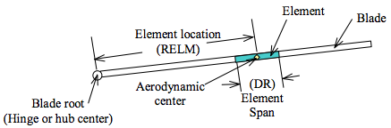
Figure 1: Blade segment nomenclature. Taken from Laino02 .

AeroDyn requires three input files to perform the aerodynamic calculations. These are, the primary data file, the airfoil data file and the wind file. Latter two are called through paths provided in primary data file. The primary data file consists of different options of models for calculation of flow influence. Additionally, it carries the information on wind reference height (hub height), convergence tolerance for induction factors, air density, kinematic air viscosity, time interval for aerodynamic calculations, and the number of blade elements per blade. For each blade element it is provided with the location, twist, span and chord length. For more clarity of the element related parameters; see blade segment terminology given in Figure 1.

The airfoil data file contains two dimensional static airfoil characteristics. It carries lift, drag and pitching moment (optional) coefficients for range of AOAs. Besides, it comprises some additional parameters pertaining to dynamic stall model. The airfoil characteristics for intermediate AOAs are obtained by linear interpolation.

The wind files in AeroDyn are used in two formats, one the hub-height wind and other the full field turbulence, which are created by either measurements or simulations. The hub-height wind files are the simple ones containing either steady or time varying wind data. The full field turbulence is generated by TurbSim program Kelley07 ; Jonkman12 , which creates two files, one the binary wind data file and other the summary file. The created wind data corresponds to all three wind components changing in time and space. The wind is sampled at frequency of 20 Hz and the turbulence is generated by a square grid spread over the whole rotor area. The velocity components at each point of the square grid are provided as function of time. The components of velocity at each blade element are obtained with linear interpolation (in terms of averaging or smoothing) in time and space Moriarty05 . For more details; see Kelley07 ; Jonkman12 .

II.2 Elemental forces

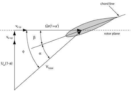
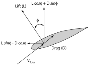
Figure 2: Scheme of force components on blade section. Angles are related to the plane of rotation. (a) Local velocities and flow angles on blade element and (b) local forces on blade element. Taken from Moriarty05 .

To determine the elemental forces on a rotating blade, the BEM method is applied on blade section as shown in Figure 2. The illustration shows the local velocities with flow angles and the acting forces on the element.

In Figure 2(a), $\phi$ represents the flow angle, $V_{\mathit{Total}}$ the relative speed, $\alpha$ the AOA and $\beta$ the combination of pitch and twist angles. The flow angle $\phi$ is the angle between the relative speed and the plane of rotation, whereas the AOA $\alpha$ is the angle between the relative speed and the chord of the blade element. The parameter $U_{\infty}$ denotes the free stream wind velocity, $\Omega$ the blade rotational speed and $r$ the local radius of the blade element. The variables $v_{\mathit{e-op}}$ and $v_{\mathit{e-ip}}$ are the out-of-plane and in-plane element velocities, respectively, originating from blade structural deflections under pronounced rotation. When the blade rotational speed is very small, the latter velocities are ignored.

The terms $U_{\infty}(1-a)$ and $\Omega r(1+\acute{a})$ are the effective axial wind and tangential blade speeds, respectively. The parameters $a$ and $\acute{a}$ are the axial and tangential induction factors, where $a$ represents the amount of reduction in axial wind speed when approaching the blade and $\acute{a}$ the amount of rotational acceleration to the blade caused by induced wake rotation opposite to the rotor rotation Mendez06 .

The induction factors are estimated using an iterative process described in the flow chart Figure 3. After initialization, the algorithm iteratively finds values fulfilling the condition expressed for $\mathit{Tol}$. The parameter $\mathit{Tol}$ is an acceptable tolerance allowed around the true values of axial and tangential induction factors. The process repeats for each element. Once the induction factors, inflow angles and AOAs converged to their final values, the acting forces are estimated for the element.

Figure 3: Flow chart to iterate for induction factors.

In flow chart Figure 3, the function $F$ represents the tip and root loss correction factors in combination, $C_{T}$ the thrust loading on the element, $\sigma$ the local solidity of the rotor, $C_{n}$ the normal force coefficient and $C_{t}$ the tangential force coefficient. The parameter $a_{\mathit{skew}}$ is the local element induction factor for skewed wake, $R$ the blade radius, $\chi$ the wake angle and $\psi$ the blade azimuth angle. For more details and derivations of the relations given in flow chart Figure 3; see Manwell09 ; Mendez06 ; Glauert35 ; Buhl05 ; Glauert26A ; Moriarty05 ; Glauert26B ; Pitt81 ; Coleman45 ; Burton11 .

III Stochastic lift and drag model

A stochastic model of the lift and drag dynamics has been developed for an advanced characterization of forces on wind turbine airfoils under unsteady wind inflow. The model parameters are derived from dynamic measurements of lift and drag forces performed for FX 79-W-151A airfoil in a wind tunnel. The turbulent inflow with intensity of 4.6% was generated using a fractal square grid, which produces the flow with typical intermittent velocity fluctuations commonly known for free field wind situations; see Luhur14 . The model extracts most of the information available in the system dynamics in terms of a dynamic response. The model reads Luhur14

$$X_{model}(k)=\\ X_{langevin}(k)+A\sin\left(\frac{2\pi k}{T}\right)\exp\left[\left(\frac{-k^{\prime}}{k_{o}}\right)^{S}\right],$$ (1)

where the first part of the equation represents the basic model and the second the extension which accounts for the oscillation effects with amplitude modulation (breathing) contained in the lift and drag time series. The parameter $X$ represents the lift and drag coefficients, $A$ the constant to fix the oscillation amplitude for lift and drag coefficients, $k$ the discrete time variable and $T$ the most dominant oscillation period of lift and drag coefficients. The exponential function in equation (1) controls the breathing of oscillation along the lift and drag time series, where $k_{o}$ is half the average breathing length, $k^{\prime}=(k~{}\mbox{mod}~{}k_{o})$ and $S$ is described as

$$S=\left\{\begin{array}[]{lr}+1,~{}\mbox{for }(2n)k_{o}<k\leq(2n+1)k_{o}\\ \\ -1,~{}\mbox{for }(2n+1)k_{o}<k\leq 2(n+1)k_{o}\;,\end{array}\right.$$ (2)

where $n=0,1,2,\ldots$.

The basic model $X_{langevin}(k)$ in equation (1) corresponds to a first order stochastic differential equation termed as Langevin equation, cf.Risken96 , expressed in discrete form as

$$X(k+1)=\\ X(k)+\tau D^{(1)}(X,\alpha)+\sqrt{\tau\tilde{F}D^{(2)}(X,\alpha)}~{}\Gamma(k),$$ (3)

where $D^{(1)}(X,\alpha)$ and $D^{(2)}(X,\alpha)$ are the drift and diffusion functions, also known as first and second Kramers-Moyal coefficients. Here $\tau$ is the integration time step and $\alpha$ the mean AOA that varies slowly compared to the fluctuations caused by turbulent inflow conditions. The parameter $\tilde{F}$ is the correction factor for diffusion function to incorporate the model extension and $\Gamma(k)$ the Gaussian white noise termed as Langevin force Risken96 with mean value $\langle\Gamma(k)\rangle=0$ and variance $\langle\Gamma^{2}(k)\rangle=2$.

The $D^{(1)}(X,\alpha)$ reflects the deterministic part of the system, whereas $D^{(2)}(X,\alpha)$ quantifies the amplitude of the stochastic fluctuations. These functions for lift and drag coefficients are parameterized as Luhur14

$$D^{(1)}(X,\alpha)=m(X-X_{o}),$$ (4)

$$D^{(2)}(X,\alpha)=\beta.$$ (5)

Here $m$ is the slope of drift function, $X$ the lift or drag coefficient, $X_{o}$ the stable fix point in $X$ where drift function is zero and $\beta$ the constant diffusion function. The optimized values for these parameters as function of mean AOAs are given in Tables 1 and 2. The intermediate values can be obtained by linear interpolation. For more details and validation of the model; see Luhur14 .

Table 1: $C_{L}$ model parameters for AOAs $0^{\circ}$ to $30^{\circ}$. The parameter $m$ is the slope of drift function, $C_{Lo}$ the stable fix point, $\beta$ the optimized diffusion function, $\tilde{F}$ the correction factor for diffusion function to incorporate the model extension, $A$ the constant to fix the oscillation amplitude, $T$ the most dominant oscillation period and $k_{o}$ half the average breathing length.

AOA	$m$	$C_{Lo}$	$\beta$	$F$	$A$	$T$	$k_{o}$	AOA	$m$	$C_{Lo}$	$\beta$	$F$	$A$	$T$	$k_{o}$
$0^{\circ}$	$-0.160$	$0.228$	$2.50e-04$	$0.329$	$0.092$	$30$	$300$	$16^{\circ}$	$-0.115$	$1.286$	$6.58e-04$	$0.500$	$0.154$	$30.25$	$300$
$1^{\circ}$	$-0.160$	$0.355$	$3.17e-04$	$0.329$	$0.105$	$30$	$300$	$17^{\circ}$	$-0.118$	$1.278$	$9.21e-04$	$0.500$	$0.175$	$30.5$	$305$
$2^{\circ}$	$-0.157$	$0.450$	$3.32e-04$	$0.330$	$0.109$	$30$	$300$	$18^{\circ}$	$-0.121$	$1.270$	$1.26e-03$	$0.500$	$0.199$	$30.75$	$300$
$3^{\circ}$	$-0.156$	$0.547$	$3.23e-04$	$0.329$	$0.107$	$30$	$300$	$19^{\circ}$	$-0.120$	$1.249$	$1.81e-03$	$0.330$	$0.290$	$31.25$	$300$
$4^{\circ}$	$-0.150$	$0.641$	$2.90e-04$	$0.329$	$0.101$	$30$	$300$	$20^{\circ}$	$-0.125$	$1.238$	$2.25e-03$	$0.330$	$0.318$	$31.33$	$300$
$5^{\circ}$	$-0.155$	$0.735$	$3.31e-04$	$0.329$	$0.107$	$30$	$300$	$21^{\circ}$	$-0.130$	$1.218$	$3.03e-03$	$0.330$	$0.348$	$32.5$	$300$
$6^{\circ}$	$-0.154$	$0.827$	$3.59e-04$	$0.330$	$0.113$	$30$	$300$	$22^{\circ}$	$-0.129$	$1.199$	$3.51e-03$	$0.330$	$0.378$	$32.5$	$300$
$7^{\circ}$	$-0.147$	$0.912$	$3.51e-04$	$0.330$	$0.113$	$30$	$300$	$23^{\circ}$	$-0.133$	$1.184$	$4.41e-03$	$0.330$	$0.415$	$32.5$	$300$
$8^{\circ}$	$-0.142$	$0.996$	$3.50e-04$	$0.330$	$0.115$	$30$	$300$	$24^{\circ}$	$-0.136$	$1.164$	$5.26e-03$	$0.329$	$0.450$	$32.33$	$300$
$9^{\circ}$	$-0.143$	$1.069$	$3.37e-04$	$0.330$	$0.114$	$30$	$300$	$25^{\circ}$	$-0.136$	$1.146$	$5.39e-03$	$0.330$	$0.460$	$32.35$	$300$
$10^{\circ}$	$-0.140$	$1.141$	$3.05e-04$	$0.329$	$0.108$	$30$	$300$	$26^{\circ}$	$-0.142$	$1.122$	$5.53e-03$	$0.329$	$0.452$	$32.5$	$300$
$11^{\circ}$	$-0.138$	$1.194$	$3.14e-04$	$0.330$	$0.113$	$30$	$300$	$27^{\circ}$	$-0.143$	$1.092$	$4.35e-03$	$0.329$	$0.410$	$32.15$	$300$
$12^{\circ}$	$-0.126$	$1.236$	$3.06e-04$	$0.329$	$0.114$	$29.9$	$300$	$28^{\circ}$	$-0.144$	$1.053$	$3.76e-03$	$0.329$	$0.376$	$32$	$290$
$13^{\circ}$	$-0.117$	$1.272$	$3.12e-04$	$0.498$	$0.104$	$29.75$	$300$	$29^{\circ}$	$-0.144$	$1.015$	$2.49e-03$	$0.329$	$0.302$	$31.8$	$285$
$14^{\circ}$	$-0.114$	$1.286$	$3.72e-04$	$0.500$	$0.113$	$29.9$	$305$	$30^{\circ}$	$-0.148$	$0.983$	$2.17e-03$	$0.329$	$0.282$	$31.45$	$325$
$15^{\circ}$	$-0.107$	$1.289$	$4.84e-04$	$0.500$	$0.136$	$30$	$300$

Table 2: $C_{D}$ model parameters for AOAs $0^{\circ}$ to $30^{\circ}$. The parameter $m$ is the slope of drift function, $C_{Do}$ the stable fix point, $\beta$ the optimized diffusion function, $\tilde{F}$ the correction factor for diffusion function to incorporate the model extension, $A$ the constant to fix the oscillation amplitude, $T$ the most dominant oscillation period and $k_{o}$ half the average breathing length.

AOA	$m$	$C_{Do}$	$\beta$	$F$	$A$	$T$	$k_{o}$	AOA	$m$	$C_{Do}$	$\beta$	$F$	$A$	$T$	$k_{o}$
$0^{\circ}$	$-0.171$	$0.052$	$1.79e-05$	$0.33$	$0.024$	$16$	$50$	$16^{\circ}$	$-0.162$	$0.162$	$9.22e-05$	$0.23$	$0.061$	$24.25$	$210$
$1^{\circ}$	$-0.190$	$0.054$	$1.67e-05$	$0.33$	$0.022$	$16$	$48$	$17^{\circ}$	$-0.163$	$0.185$	$1.37e-04$	$0.23$	$0.074$	$24.5$	$210$
$2^{\circ}$	$-0.196$	$0.055$	$1.79e-05$	$0.329$	$0.022$	$17$	$50$	$18^{\circ}$	$-0.172$	$0.210$	$2.22e-04$	$0.23$	$0.091$	$24.75$	$210$
$3^{\circ}$	$-0.190$	$0.056$	$1.90e-05$	$0.33$	$0.023$	$17$	$50$	$19^{\circ}$	$-0.169$	$0.240$	$3.45e-04$	$0.23$	$0.114$	$25.25$	$210$
$4^{\circ}$	$-0.192$	$0.058$	$2.12e-05$	$0.33$	$0.024$	$17.5$	$100$	$20^{\circ}$	$-0.176$	$0.270$	$5.17e-04$	$0.23$	$0.137$	$25.25$	$300$
$5^{\circ}$	$-0.192$	$0.060$	$2.24e-05$	$0.33$	$0.025$	$18$	$105$	$21^{\circ}$	$-0.169$	$0.300$	$7.03e-04$	$0.23$	$0.157$	$26$	$210$
$6^{\circ}$	$-0.197$	$0.060$	$2.55e-05$	$0.33$	$0.026$	$18.5$	$90$	$22^{\circ}$	$-0.185$	$0.336$	$1.08e-03$	$0.23$	$0.191$	$25.5$	$210$
$7^{\circ}$	$-0.203$	$0.065$	$2.86e-05$	$0.23$	$0.030$	$23.8$	$95$	$23^{\circ}$	$-0.185$	$0.369$	$1.45e-03$	$0.23$	$0.217$	$25.66$	$210$
$8^{\circ}$	$-0.200$	$0.068$	$3.20e-05$	$0.23$	$0.031$	$23.85$	$120$	$24^{\circ}$	$-0.191$	$0.402$	$2.01e-03$	$0.23$	$0.245$	$25.65$	$300$
$9^{\circ}$	$-0.206$	$0.072$	$3.56e-05$	$0.23$	$0.032$	$23.85$	$120$	$25^{\circ}$	$-0.193$	$0.431$	$2.38e-03$	$0.23$	$0.278$	$25.65$	$300$
$10^{\circ}$	$-0.206$	$0.077$	$3.89e-05$	$0.23$	$0.034$	$23.85$	$95$	$26^{\circ}$	$-0.188$	$0.467$	$2.65e-03$	$0.23$	$0.302$	$25.8$	$300$
$11^{\circ}$	$-0.200$	$0.083$	$4.19e-05$	$0.23$	$0.036$	$23.9$	$210$	$27^{\circ}$	$-0.194$	$0.503$	$2.81e-03$	$0.23$	$0.301$	$25.5$	$300$
$12^{\circ}$	$-0.198$	$0.092$	$4.50e-05$	$0.23$	$0.038$	$23.9$	$210$	$28^{\circ}$	$-0.195$	$0.552$	$2.63e-03$	$0.23$	$0.291$	$25.5$	$305$
$13^{\circ}$	$-0.192$	$0.108$	$4.89e-05$	$0.23$	$0.039$	$23.9$	$210$	$29^{\circ}$	$-0.195$	$0.590$	$2.33e-03$	$0.23$	$0.271$	$25.3$	$250$
$14^{\circ}$	$-0.184$	$0.123$	$5.92e-05$	$0.23$	$0.045$	$24$	$210$	$30^{\circ}$	$-0.198$	$0.623$	$2.04e-03$	$0.23$	$0.255$	$25.1$	$325$
$15^{\circ}$	$-0.175$	$0.140$	$6.89e-05$	$0.23$	$0.050$	$24.15$	$210$

IV Model integration into AeroDyn

The stochastic lift and drag model described in Section III is integrated into AeroDyn to obtain aerodynamic forces with local dynamics on the rotating blade. The model is added in form of a routine based on model equation (1) as an alternate to static airfoil data files used by the classical BEM model in AeroDyn. The characteristics of model related parameters given in Tables 1 and 2 are imported as input files to the model routine. The axial and tangential induction factors are estimated (using mean lift and drag coefficients) through an iterative procedure described in Figure 3.

Figure 4: Flow chart for aerodynamic calculations.

IV.1 Numerical setup

Before starting the aerodynamic computations, the AeroDyn input files described in Section II.1 are set up for intended options of computations. In primary file the wind reference height, air density and air kinematic viscosity are taken as 42.7 m, 1.225 kg/m³ and 1.464e^-5 m²/s, respectively.

The aerodynamic calculations are performed for a three-bladed rotor having radius of 13.76 m. The blade is divided into 10 equal segments along the radius. The local design specifications for each element are given in Table 3 containing the element nodal radius (from blade hub centre to the centre of element), twist angle, span and chord length. All three blades have the same distribution yielding identical aerodynamics for same pitch angle -1^∘. The elemental pitch can be obtained by adding the blade pitch angle to the element’s local twist angle. The computations are carried out for all 10 elements; however, the results here are presented for element number 5 only to avoid the repetition of similar statistics.

Table 3: Blade local design parameters along the span. Taken from FAST archive (Test03_AD.ipt).

No. of	Nodal	Twist	Element	Chord
element	radius [m]	angle [∘]	span [m]	length [m]
$1$	$1.81$	$5.80$	$1.26$	$0.86$
$2$	$3.07$	$5.20$	$1.26$	$1.05$
$3$	$4.33$	$4.66$	$1.26$	$1.15$
$4$	$5.58$	$3.73$	$1.26$	$1.12$
$5$	$6.84$	$2.64$	$1.26$	$1.05$
$6$	$8.10$	$1.59$	$1.26$	$0.98$
$7$	$9.36$	$0.73$	$1.26$	$0.89$
$8$	$10.61$	$0.23$	$1.26$	$0.78$
$9$	$11.87$	$0.08$	$1.26$	$0.65$
$10$	$13.13$	$0.03$	$1.26$	$0.49$

Since the model is based on aerodynamic characteristics of an FX 79-W-151A, for comparison purpose the airfoil data file of AeroDyn is replaced with measured aerodynamic characteristics of this airfoil (for measurement details see Luhur14 ).

For wind input, the full field turbulence simulated binary wind data file is used. The file represents all three components of the wind vector created with TurbSim program. The components are variable in time and space obtained at each element each moment by subroutine interpolations. A summary of the meteorological parameters of the wind data file is given in Table 4.

Table 4: Meteorological boundary conditions of the wind data file. Taken from FAST archive.

Turbulence model used	:	IEC von Karman
IEC standard	:	IEC 61400-1 Ed. 2: 1999
Turbulence characteristic	:	A
IEC turbulence type	:	Normal turbulence model
Reference height (hub-height)	:	42.7 m
Reference wind speed (mean speed at hub-height)	:	12 m/s
Power law exponent	:	0.2
Surface roughness length	:	0.03
Interpolated hub-height turbulence intensity	:	15%

It has to be stressed that the model parameters have been derived from wind tunnel measurements in fractal square grid generated stationary turbulence, while the simulation uses synthetic turbulent inflow according to Table 4. To compensate at least partially for the different flow situations, the diffusion function of the basic model equation (3) is multiplied with a correction factor obtained by dividing synthetic wind input interpolated hub-height turbulence intensity with fractal square grid generated turbulence intensity. Due to the high complexity of turbulence, this can nevertheless not ensure completely comparable flow situations.

As described in Section II, AeroDyn can not be operated independently, but has to be initiated by a dynamic analysis code. Here it is invoked by FAST, which uses a combined modal and multi-body dynamics representation. In FAST, the wind turbine blades and tower are modeled by applying the linear representation considering small deflections with mode shapes (degrees of freedom (DOF)) listed in Table 5 Jonkman05 ; Cordle10 . FAST collects the basic information from its primary input file containing the details of wind turbine operating conditions and the basic geometry. For additional information such as blade properties, tower properties, furling properties, wind time histories and the aerodynamic characteristics, FAST reads some supplementary files Jonkman05 .

Table 5: Wind turbine mode shapes and configuration. Taken from FAST archive (Test03.fst).

Number of blades used	:	3
First and second flap-wise blade mode DOF	:	Yes
First edge-wise blade mode DOF	:	Yes
Drivetrain rotational-flexibility DOF	:	Yes
Generator DOF	:	Yes
Yaw DOF	:	Yes
First and second fore-aft tower bending-mode DOF	:	Yes
First and second side-to-side tower bending-mode DOF	:	Yes
Initial or fixed rotor speed	:	53.33 rpm
Blade tip radius from rotor apex	:	13.76 m
Hub radius from rotor apex to blade root	:	1.18 m
Tower height from ground level to rotor-shaft (hub-height)	:	42.7 m

Once FAST calls AeroDyn and exchanges the information on the model status including elemental pitch and velocities, AeroDyn starts to compute the elemental aerodynamic forces. The velocity components are expressed normal and tangential to the plane of rotation.

IV.2 Results

Results are achieved for a blade element following the numerical setup described in Section IV.1. The force calculations are performed using the classical BEM, dynamic stall and stochastic models according to procedure given in flow chart Figure 4. The TurbSim generated synthetic wind is used as an input to AeroDyn. Simulations are performed for 10 realizations of 10 minutes of wind input. The synthetic wind, containing irregular speed and irregular turbulence level, led to strong fluctuations in local wind components and AOA as expected; see Figure 2. The figure portrays the complex fluctuations of the axial velocity component experienced by the blade element and its effect on AOA dynamics; compare Stoevesandt09 . The variations in velocity component are proportional to the AOA, i.e., the higher the wind fluctuations, the higher the AOA variation. A pronounced oscillation at $T=1.13$ s is visible in Figure 2, which possibly stems from boundary layer shear effects, as the tower-blade interaction was not included in the simulations .

The blade aerodynamics is function of the AOA, therefore, a change in AOA means a change in aerodynamic forces; compare Figure 2(b) with Figure 6. Figure 6 shows the resulting aerodynamic forces behavior for the selected element, where the force coefficient signals obtained with classical BEM represent the mean force dynamics as expected, being dependent on mean aerodynamic characteristics of the airfoil. The force coefficient signals achieved with the dynamic stall model represent the force dynamics with small fluctuations around the mean, while the force coefficient signals contributed by the stochastic model represent the force dynamics with extended local dynamics around the mean compared to the dynamic stall model. The means of the dynamic stall and stochastic models’ local force dynamics along the signals match almost perfectly with the classical BEM model force signals.

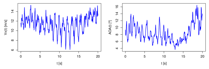
Figure 5: Excerpt of local axial wind velocity component and AOA time series for a blade element. (a) Local axial wind component experienced by the blade element and (b) local AOA. Note the rotor oscillation at $T=1.13$ s in (a) and (b), which possibly stems from ground boundary layer shear effects. The oscillation in (b) is less visible because of short excerpt; however, it is present at the same period.

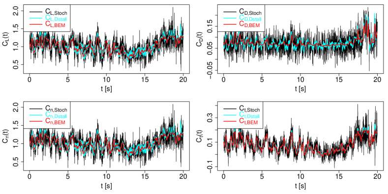
Figure 6: Excerpt of the stochastic model, the dynamic stall model and the classical BEM model aerodynamic forces time series for a blade element. Black represents the stochastic model forces, cyan the dynamic stall model forces and red the classical BEM model forces (color online). (a) $C_{L,Stoch}(t)$, $C_{L,Dstall}(t)$ and $C_{L,BEM}(t)$, (b) $C_{D,Stoch}(t)$, $C_{D,Dstall}(t)$ and $C_{D,BEM}(t)$, (c) $C_{n,Stoch}(t)$, $C_{n,Dstall}(t)$ and $C_{n,BEM}(t)$, and (d) $C_{t,Stoch}(t)$, $C_{t,Dstall}(t)$ and $C_{t,BEM}(t)$.

In order to investigate the quality of the stochastic model results, their statistical properties are compared with the classical BEM and dynamic stall models’ results in terms of increment probability density functions (PDFs). The increments in our case are the differences of an aerodynamic force over a specific time lag described as Morales12

$$\delta{x}(t,\tau)=x(t+\tau)-x(t).$$ (6)

The increment statistics are basically two-point statistics, which determine the nature of a parameter variation against a selected time lag. Using equation (6), the increment signals of the aerodynamic forces are derived for different time lags. Increment PDFs of the stochastic, dynamic stall and classical BEM models’ results for different time lags are shown in Figures 7, 8 and 9, respectively.

For quantitative comparison, further kurtosis and standard deviations of the increment signals have been estimated. The kurtosis is calculated using the expression

$$\gamma_{{}_{2}}=\frac{\langle(x-\bar{x})^{4}\rangle}{\sigma_{x}^{4}}-3,$$ (7)

where $\gamma_{{}_{2}}$ is the excess kurtosis, $\langle(x-\bar{x})^{4}\rangle$ the fourth moment around the mean and $\sigma_{x}^{4}$ the square of the variance of the probability distribution. The $\gamma_{{}_{2}}=0$ resemble a normal distribution, $\gamma_{{}_{2}}>0$ a distribution with sharp peak and long heavy tails, and $\gamma_{{}_{2}}<0$ a distribution with round peak and short light tails. The excess kurtosis is a measure of the deviation of PDF shape from the normal distribution.

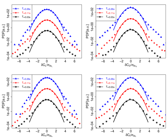
Figure 7: Increment PDFs of the stochastic model force coefficients for a blade element at time lags $\tau=(0.03,0.11,0.26)$ s in ascending order from bottom to top. The PDFs are added with a Gaussian fit having identical standard deviation (solid line) and shifted vertically for clarity of the display. The force coefficients are normalized with their standard deviations. (a) Lift coefficient increment $\delta{C_{L}}(t,\tau)$ PDFs, (b) Drag coefficient increment $\delta{C_{D}}(t,\tau)$ PDFs, (c) Normal force coefficient increment $\delta{C_{n}}(t,\tau)$ PDFs, and (d) Tangential force coefficient increment $\delta{C_{t}}(t,\tau)$ PDFs.

Table 6: Kurtosis and standard deviation of the increment signals of the stochastic model force coefficients at different time lags.

Inrement	Kurtosis				Standard deviation
$\tau$[s]	$\delta{C_{L}}$	$\delta{C_{D}}$	$\delta{C_{n}}$	$\delta{C_{t}}$	$\delta{C_{L}}$	$\delta{C_{D}}$	$\delta{C_{n}}$	$\delta{C_{t}}$
$0.03$	$1.80$	$1.37$	$1.66$	$3.04$	$0.26$	$0.06$	$0.26$	$0.08$
$0.11$	$0.98$	$1.01$	$0.90$	$1.59$	$0.29$	$0.06$	$0.28$	$0.09$
$0.26$	$0.44$	$1.42$	$0.40$	$0.96$	$0.31$	$0.06$	$0.30$	$0.09$

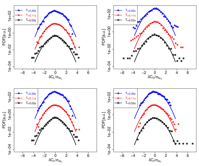
Figure 8: Increment PDFs of the dynamic stall model force coefficients for a blade element at time lags $\tau=(0.03,0.11,0.26)$ s in ascending order from bottom to top. The PDFs are added with a Gaussian fit having identical standard deviation (solid line) and shifted vertically for clarity of the display. The force coefficients are normalized with their standard deviations. (a) Lift coefficient increment $\delta{C_{L}}(t,\tau)$ PDFs, (b) Drag coefficient increment $\delta{C_{D}}(t,\tau)$ PDFs, (c) Normal force coefficient increment $\delta{C_{n}}(t,\tau)$ PDFs, and (d) Tangential force coefficient increment $\delta{C_{t}}(t,\tau)$ PDFs.

Table 7: Kurtosis and standard deviation of the increment signals of the dynamic stall model force coefficients at different time lags.

Inrement	Kurtosis				Standard deviation
$\tau$[s]	$\delta{C_{L}}$	$\delta{C_{D}}$	$\delta{C_{n}}$	$\delta{C_{t}}$	$\delta{C_{L}}$	$\delta{C_{D}}$	$\delta{C_{n}}$	$\delta{C_{t}}$
$0.03$	$1.38$	$2.23$	$1.40$	$1.01$	$0.06$	$0.01$	$0.06$	$0.01$
$0.11$	$0.06$	$1.84$	$0.07$	$0.33$	$0.11$	$0.03$	$0.11$	$0.03$
$0.26$	$-0.09$	$1.34$	$-0.09$	$-0.05$	$0.17$	$0.04$	$0.17$	$0.05$

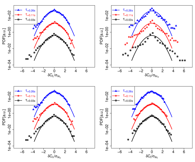
Figure 9: Increment PDFs of the classical BEM model force coefficients for a blade element at time lags $\tau=(0.03,0.11,0.26)$ s in ascending order from bottom to top. The PDFs are added with a Gaussian fit having identical standard deviation (solid line) and shifted vertically for clarity of the display. The force coefficients are normalized with their standard deviations. (a) Lift coefficient increment $\delta{C_{L}}(t,\tau)$ PDFs, (b) Drag coefficient increment $\delta{C_{D}}(t,\tau)$ PDFs, (c) Normal force coefficient increment $\delta{C_{n}}(t,\tau)$ PDFs, and (d) Tangential force coefficient increment $\delta{C_{t}}(t,\tau)$ PDFs.

Table 8: Kurtosis and standard deviation of the increment signals of the classical BEM model force coefficients at different time lags.

Inrement	Kurtosis				Standard deviation
$\tau$[s]	$\delta{C_{L}}$	$\delta{C_{D}}$	$\delta{C_{n}}$	$\delta{C_{t}}$	$\delta{C_{L}}$	$\delta{C_{D}}$	$\delta{C_{n}}$	$\delta{C_{t}}$
$0.03$	$1.37$	$6.62$	$1.42$	$0.72$	$0.03$	$0.01$	$0.03$	$0.01$
$0.11$	$0.78$	$4.43$	$0.81$	$0.28$	$0.08$	$0.02$	$0.08$	$0.03$
$0.26$	$0.49$	$3.31$	$0.51$	$-0.02$	$0.14$	$0.03$	$0.14$	$0.05$

Figure 7 presents the increment PDFs for stochastic model results, where all four aerodynamic force coefficients look similar at all three time lags except some differences at the tails. All PDFs almost resemble the normal distribution shape up to $\pm 3\sigma$; compare with added Gaussian fit. At the tails, the PDFs deviate from the Gaussian distribution and show intermittent behavior. To quantify for these shapes, the kurtosis and standard deviations of the increment signals have been estimated as given in Table 6. The estimations show slight to pronounced higher positive kurtosis for all four aerodynamic force coefficient signals at the selected time lags, meaning that the increment PDFs have slight to pronounced heavier tails. The main reason for this effect seem to be the non-linear lift and drag characteristics of the airfoil over AOA. The standard deviations of the increment signals in each force coefficient case at all three time lags are close to each other in magnitude; see Table 6.

Figure 8 presents the increment PDFs for dynamic stall model results. In this case, the increment PDFs except those of the drag coefficient, resemble similar shape with minor differences at the tails. The drag increment PDFs present heavier tails compared to other three force coefficients. However, the increment PDFs of all forces correspond fairly to the normal distribution up to $\pm 3\sigma$ (compare with added Gaussian fit) at all three time lags. The estimated kurtosis values given in Table 7 indicate very slight to pronounced heavier tails for all force coefficient signals except almost no deviations in case of the lift, normal force and tangential force coefficients at higher time lags. The contribution of pronounced intermittency in the force signals is believed to stem from the same phenomenon as described in stochastic model case. The standard deviations of the all three increment signals in each force case depict increase with an increase in time lag; see Table 7.

Similarly, Figure 9 shows the increment PDFs for classical BEM model results. Here, except drag coefficient, the increment PDFs of other three force coefficients portray similar shape for same time lags. The increment PDFs of the lift, normal force and tangential force coefficients, resemble fairly the normal distribution shape up to $\pm 3\sigma$ (compare with added Gaussian fit), whereas the drag coefficient correspond to the intermittent shape. The evaluated kurtosis given in Table 8 indicate strong heavier tails for drag coefficient increment PDFs at all three time lags. The other three force coefficients show slight to pronounced heavier tails for all three time lags except negligible lighter tails for higher time lag in case of the tangential force coefficient. The contribution of strong intermittency in the drag coefficient as well as slight to pronounced intermittency in other force coefficients can probably be addressed to the same phenomenon as in the stochastic model case. The standard deviations of the force coefficient signals follow the same behavior as in the dynamic stall model case above; compare Tables 7 and 8.

V Discussion and outlook

The stochastic model of the lift and drag dynamics for an airfoil FX 79-W-151A described in Section III has been integrated to AeroDyn in the context of BEM wake model. The forces are obtained through the classical BEM, dynamic stall and stochastic models used by AeroDyn. For wind input, the full field turbulence simulated binary wind data is used. The forces are estimated for 10 blade elements; however, the results are analyzed here for one element only to avoid the repetition of similar statistics. With this ansatz it could be shown that local, short-time fluctuations of aerodynamic forces can be integrated as a stochastic model into a current WEC simulation tool.

The comparison of force time series given in Figure 6 show that the classical BEM model force coefficient signals represent the mean dynamics as expected, being dependent on mean aerodynamic characteristics of the airfoil. The dynamic stall model forces reflect small fluctuations around the mean, whereas the stochastic model introduces additional extended local force dynamics around the mean. The means of the local force dynamics achieved with dynamic stall and stochastic models seem to coincide with the classical BEM model force coefficient signals. Nevertheless, the stochastic model contributes additional extended dynamic response in terms of local force fluctuations, which is neglected by the classical BEM model fully and partially by the dynamic stall model.

The statistics of the stochastic and dynamic stall models presented in Figures 7 and 8 show good consistency. The increment PDFs of stochastic model force coefficients resemble normal distributions up to $\pm 3\sigma$. Similarly, the increment PDFs of dynamic stall model force coefficients also resemble fairly a normal distribution up to $\pm 3\sigma$. Both the stochastic and dynamic stall models’ force increment PDFs yield slight to pronounced intermittency due to the non-linear lift and drag characteristics of the airfoil over AOA. The magnitude of the standard deviations of the stochastic model force increment signals is significantly higher that of the dynamic stall model; compare Tables 6 and 7. That is because the dynamic stall model forces possess smaller magnitudes of local fluctuations compared to the stochastic model. Moreover, the behavior of the standard deviations of the increment signals is different in both the stochastic and dynamic stall model cases. The standard deviations in the stochastic model case seem nearly stable for all time lags, whereas for the dynamic stall model case they are proportional to time lags.

Similarly, the comparison of statistics between stochastic and classical BEM models given in Figures 7 and 9 also reflect good consistency except for the drag coefficient. The increment PDFs of the stochastic and classical BEM models’ force coefficients resemble normal distributions up to $\pm 3\sigma$ besides the BEM model drag coefficient. The intermittency in this range in the stochastic model drag coefficient is mostly covered by Gaussian fluctuations. The strong intermittency in the BEM model drag coefficient as well as slight to pronounced intermittency in other force coefficients in both the stochastic and classical BEM model cases can probably be addressed to the same reason described above. The magnitude of the stochastic model force standard deviations is larger than the classical BEM model forces; compare Tables 6 and 8. The reason is the extended local force dynamics in case of stochastic model. The behavior of the standard deviations of the increment signals between stochastic and classical BEM models is very similar as observed between stochastic and dynamic stall models.

As described in Section IV.1 the stochastic model parameters have necessarily been obtained under different conditions than the simulations carried out here. As a first compensation, the diffusion function has been scaled according to the interpolated hub-height turbulence intensity of wind input taken for the present computations. This can; however, not guarantee completely comparable flow situations. Therefore, the comparability of results between the stochastic model and the dynamic stall and BEM models is limited at the current state. For better quantitative comparison of stochastic versus dynamic stall and BEM models, in the future the stochastic model parameters have to be derived from measurements in more realistic flow situations at wind turbine airfoils. Also a comparison to load measurements at a real WEC should be performed.

Additionally, at the present state, the stochastic model could not generate the expected intermittency in the resulting forces, which is probably washed-out by the Gaussian noise term of the model. To improve this point, multiplicative noise may be introduced to achieve intermittency in the forces corresponding to intermittent properties of atmospheric flows, which is currently work in progress.

The stochastic model is being developed to extract and provide more complete local loading information on wind turbine blades, which could lead to an optimized rotor design under turbulent wind inflow. Here we have shown that the local force dynamics can be provided by a stochastic model integrated into existing BEM codes used by aerodynamic models such as AeroDyn. Further work will have to include more realistic model parameterization and corresponding experiments to allow for quantitative evaluation of the results.

- (1) GWEC, 2013. Global Wind Report-Annual Market Update 2012. Technical report, Global Wind Energy Council, Brussels, Belgium, April.
- (2) Vermeer, L. J., Sørensen, J. N., and Crespo, A., 2003. “Wind turbine wake aerodynamics”. Progress in Aerospace Sciences, 39(6–7), August–October, pp. 467–510. doi: 10.1016/S0376–0421(03)00078–2.
- (3) Liu, S., and Janajreh, I., 2012. “Development and application of an improved blade element momentum method model on horizontal axis wind turbines”. International Journal of Energy and Environmental Engineering, 3, October, pp. 30 (10 pages). doi: 10.1186/2251–6832–3–30.
- (4) Åhlund, K., 2004. Investigation of the NREL NASA/Ames Wind Turbine Aerodynamics Database. Scientific report FOI-R–1243–SE, Swedish Defence Research Agency, Stockholm, Sweden, June.
- (5) Hansen, M. O. L., and Madsen, H. A., 2011. “Review paper on wind turbine aerodynamics”. Journal of Fluids Engineering, 133(11), October, p. 114001 (12 pages). doi: 10.1115/1.4005031.
- (6) Jonkman, J. M., and Buhl Jr., M. L., 2005. FAST User’s Guide. Technical report NREL/EL-500-38230, National Renewable Energy Laboratory, Golden, Colorado, USA, August.
- (7) Laino, D. J., and Hansen, A. C., 2003. User’s Guide to the Wind Turbine Dynamics Computer Program YawDyn. Technical report prepared for NREL under subcontract No. TCX-9-29209-01, University of Utah, Salt Lake City, USA, January.
- (8) Laino, D. J., and Hansen, A. C., 2001. User’s Guide to the Computer Software Routines AeroDyn Interface for ADAMS. Technical report prepared for NREL under subcontract No. TCX-9-29209-01, University of Utah, Salt Lake City, USA, September.
- (9) Mulski, S., 2012. “Simpack multi-body simulation”. In Proceedings of the Wind and Drivetrain Conference, Hamburg, Germany, SIMPACK AG.
- (10) Buhl Jr., M. L., and Manjock, A., 2006. A Comparison of Wind Turbine Aeroelastic Codes Used for Certification. Conference paper NREL/CP-500-39113, National Renewable Energy Laboratory, Golden, Colorado, USA, January.
- (11) Øye, S., 1999. FLEX5 User Manual. Technical report, Danske Techniske Hogskole.
- (12) Moriarty, P. J., and Hansen, A. C., 2005. AeroDyn Theory Manual. Technical report NREL/EL-500-36881, National Renewable Energy Laboratory, Golden, Colorado, USA, January.
- (13) Weinzierl, G., 2011. “A BEM Based Simulation-Tool for Wind Turbine Blades with Active Flow Control Elements.”. Diploma Thesis, Technical University of Berlin, Berlin, Germany, April.
- (14) Luhur, M. R., Peinke, J., Schneemann, J., and Wächter, M., 2014. “Stochastic modeling of lift and drag dynamics under turbulent wind inflow conditions”. Wind Energy, doi: 10.1002/we.1699, published online.
- (15) Laino, D. J., and Hansen, A. C., 2002. User’s Guide to the Wind Turbine Aerodynamics Computer Software AeroDyn. Technical report prepared for NREL under subcontract No. TCX-9-29209-01, University of Utah, Salt Lake City, USA, December.
- (16) Kelley, N. D., and Jonkman, B. J., 2007. Overview of the TurbSim Stochastic Inflow Turbulence Simulator. Technical report NREL/TP-500-41137, National Renewable Energy Laboratory, Golden, Colorado, USA, April.
- (17) Jonkman, B. J., and Kilcher, L., 2012. TurbSim User’s Guide: Version 1.06.00. Technical report draft version, National Renewable Energy Laboratory, Golden, Colorado, USA, September.
- (18) Méndez, J., and Greiner, D., 2006. “Wind blade chord and twist angle optimization by using genetic algorithms”. In Proceedings of the Fifth International Conference on Engineering Computational Technology, B. Topping, G. Montero, and R. Montenegro, eds., Las Palmas de Gran Canaria, Spain, Civil-Comp Press.
- (19) Note1. The azimuth angle describes the blade angular position in one cycle measured in clockwise direction such that it is zero when the blade is pointing vertically downwards.
- (20) Manwell, J. F., McGowan, J. G., and Rogers, A. L., 2009. Wind Energy Explained: Theory, Design and Application, ed. John Wiley & Sons, Chichester, UK.
- (21) Glauert, H., 1935. Airplane Propellers, aerodynamic theory w.f. durand ed. Springer, Berlin, Germany.
- (22) Buhl Jr., M. L., 2005. A new empirical relationship between thrust coefficient and induction factor for the turbulent windmill state. Technical report NREL/TP-500-36834, National Renewable Energy Laboratory, Golden, Colorado, USA, August.
- (23) Glauert, H., 1926. A General Theory of the Autogyro, volume 1111 of reports and memoranda ed. British ARC, UK.
- (24) Glauert, H., 1926. The Analysis of Experimental Results in the Windmill Brake and Vortex Ring States of an Airscrew, volume 1026 of reports and memoranda ed. HMSO, London, UK.
- (25) Pitt, D. M., and Peters, D. A., 1981. “Theoretical prediction of dynamic-inflow derivatives”. Vertica, 5(1), March, pp. 21–34.
- (26) Coleman, R. P., Feingold, A. M., and Stempin, C. W., 1945. Evaluation of the Induced-Velocity Field of an Idealized Helicopter Rotor. Wartime report NACA ARR L5E10, National Advisory Committee for Aeronautics, Washington, USA, June.
- (27) Burton, T., Sharpe, D., Jenkins, N., and Bossanyi, E., 2011. Wind Energy Handbook, ed. John Wiley & Sons, Chichester, UK.
- (28) Risken, H., 1996. The Fokker-Planck Equation, ed. Springer, Berlin, Germany.
- (29) Cordle, A., 2010. State-of-the-art in design tools for floating offshore wind turbines. Deliverable report under contract No. 019945 (SES6), UpWind project, Bristol, UK, March.
- (30) Stoevesandt, B., and Peinke, J., 2009. “Changes in angle of attack on blades in the turbulent wind field”. In Proceedings of EWEC 2009, Parc Chanot, Marseille, France.
- (31) Note2. The appearance of harmonics of the 1P period seems to be typical for the rotating frame of reference of the rotor Jonkman2014 .
- (32) Morales, A., Wächter, M., and Peinke, J., 2012. “Characterization of wind turbulence by higher order statistics”. Wind Energy, 15(3), April, pp. 391–406. doi: 10.1002/we.478.
- (33) Jonkman, J., 2014. Personal communication, National Renewable Energy Laboratory, USA.