A coordinated wavefunction for the ground state of liquid ⁴He

Abstract

We present a variational ansatz for the ground state of a strongly correlated Bose system. This ansatz goes beyond the Jastrow-Feenberg functional form and explicitly enforces coordination shells in the structure of the wavefunction. We apply this ansatz to liquid helium-4 with a simple three-variable parametrization of the pair functions. The optimized wavefunction is found to give an excellent description of the mid-range correlations in the fluid. We also demonstrate the possibility to use this ansatz to study inhomogeneous systems. The phase separation and free surface emerge naturally in this wavefunction, even though it is constructed of short-range two-body functions and does not contain one-body terms. Because no explicit description of the surface is necessary, this provides a powerful description tool for cluster states.

I Introduction

The interest in the microscopic nature of the ground state of liquid ⁴He has drawn attention for over half a century and has shaped the development of many aspects of the quantum many-body theory Bishop et al. (2000). The question continues to be on interest, especially as new correlated bosonic systems are becoming the subject of an experiment, including the cold atomic gases Vassen et al. (2012); Ketterle (2002); Greywall (1993); Nakashima et al. (2011). An explicit and numerically efficient expression for the many-body wavefunction also has a practical use in computer calculations. A good approximation to the ground state reduces the numerical costs and improves the statistical accuracy of the true ground state results obtained with the diffusion Monte Carlo Anderson (1980); Ceperley and Alder (1980) as well as the path-integral ground state Monte Carlo Sarsa et al. (2000); Galli and Reatto (2003); Cuervo et al. (2005); Rota et al. (2010) methods.

The variational ansatz for liquid ⁴He has followed the path of improving the Jastrow-Feenberg form of the wavefunction Feenberg (1974); Chang and Campbell (1977),

$$\psi(\bm{r}_{1},\dots,\bm{r}_{N})=\prod_{i<j}e^{\frac{1}{2}u_{2}(\bm{r}_{i}-\bm{r}_{j})}\prod_{i<j<k}e^{\frac{1}{2}u_{3}(\bm{r}_{i}-\bm{r}_{j},\bm{r}_{j}-\bm{r}_{k},\bm{r}_{k}-\bm{r}_{i})}\dots,$$ (1)

where $N$ is the number of atoms, and the $k$-body correlation factors $u_{k}$ must have proper symmetry under the exchange of particles. Because each successive term in Eq. (1) increases the the numerical complexity by an additional factor of $N$, one is in practice limited to two- and three-body terms. Limiting Eq. (1) to two-body factors results in the Jastrow function Bijl (1940); Jastrow (1955). In an early work, McMillan McMillan (1965) and Schiff and Verlet Schiff and Verlet (1967) used a Jastrow function with the two-body function $u_{2}=-{\left({b}/{r}\right)}^{5}$. Parameter $b$ was determined variationally. The McMillan function captures the most significant features of the system caused by the core of the interparticle potential and it continues to be used successfully as a guiding function for projector Monte CarloRota et al. (2010); Vranješ et al. (2005); Cazorla et al. (2012). Successive improvements in the ground state of helium refined the two- and, later, three- body factors in the form (1). Published progress on this topic is too numerous to cover in any detail here. Relevant to this work, we note the addition of the mid-range correlation Michelis and Reatto (1974); Reatto (1979) which among other things allowed to replicate the first correlation peak of the pair distribution function $g(r)$; the addition of long-range terms in the two-body function $u_{2}$ that allows to account for the long-wavelength zero-point phonons Reatto and Chester (1967); Francis et al. (1970); the computation of $u_{2}$ based on the maximum overlap with the true ground-state Masserini and Reatto (1984, 1987); and finally, a detailed optimization of the pair factors expanded in terms of the pair scattering eigenstates Vitiello and Schmidt (1992, 1999) which along with the inclusion of the three-body factors allowed to account for nearly all the correlation energy. The success of the above works came at the expense of the increased complexity and and the number of variational parameters that are needed to accurately describe the functions $u_{k}$. The general functional form of Eq. (1), though, remained unchanged.

The development of the shadow wavefunction (SWF) methods Vitiello et al. (1988); Reatto and Masserini (1988) has to a large degree overtaken the development of the wavefunction for liquid helium. The SWF allows to account for the correlations missed by the Jastrow function, and results in an excellent description in terms of both energy and structure MacFarland et al. (1992, 1994) of ⁴He. Relevant to this work, we notice that SWF can support self-bound states of liquid ⁴He Zhang et al. (1994). Shadow wavefunction accounts for correlations via integrals on auxiliary (shadow) variables. The inclusion of the shadow variables may be seen as going beyond the Jastrow-Feenberg form of Eq. (1). However, the integrals on the shadow variables must be taken numerically by a Monte Carlo scheme, and in this sense shadow wavefunction is not explicit, partially limiting its adoption in quantum Monte Carlo.

We will present a variational ansatz for the ground state of liquid ⁴He which is build upon the Jastrow wavefunction but goes beyond the general functional form of Eq. (1). This ansatz allows to explicitly control the mid-range structure of the liquid and results in a stark improvement of the atomic pair distribution already with a three-parameter wavefunction. The wavefunction is presented in Section II and the computational results are shown in Section III. Section IV presents results for inhomogeneous systems, followed by a discussion.

II The coordinated wavefunction

II.1 Variational ansatz

Our proposed wavefunction consists of a product of the Jastrow function (limiting Eq. (1) to two-body terms) and of the additional term to which we refer as the “coordination term”. The wavefunction has the following form,

$$\psi_{JC}(\bm{r}_{1},\dots,\bm{r}_{N})=\prod_{i<j}e^{\frac{1}{2}u_{2}(|\bm{r}_{i}-\bm{r}_{j}|)}\prod_{i}\sum_{j\neq i}y_{2}(|\bm{r}_{i}-\bm{r}_{j}|).$$ (2)

The factors $y_{2}(r)$ must vanish at large distances. At short distances, $y_{2}$ is expected to raise to a constant.

The effect of the coordination term in (2) can be seen by inspection. Suppose the function $y_{2}(r)$ vanishes for distances $r$ beyond the mean interparticle distance. In this case, $y_{2}(r_{ij})$ will have significant value only for the pairs of immediate neighbors $\langle i,j\rangle$. On the other hand, the number of neighbors for each atom is limited by the presence of the repulsive core and by the Jastrow part of the wavefunction. Thus the overall number of non-vanishing terms $y_{2}(r_{ij})$ in the system is, roughly speaking, fixed. Under such a restraint, the product of sums in the coordination part of Eq. (2) is maximized when all sums are equal to each other. That is, the non-vanishing values of $y_{2}(r_{ij})$ are distributed equally between the products. The wavefunction $\psi_{JC}$, while constructed only of pairwise functions, has a “global” property in that it explicitly demands that each atom in the system has an equal expected number of immediate neighbors. As we will see, this allows to improve the mid-range properties of the system independently of the Jastrow factor.

II.2 Inspiration and origin

The inspiration for the coordinated wavefunction $\psi_{JC}$ comes from the symmetrized Bose-solid wavefunction proposed by Cazorla et al. Cazorla et al. (2009). This symmetrical solid wavefunction does an excellent work describing quantum Bose solid, both variationally Lutsyshyn et al. (2014) and as a guiding function for importance sampling in quantum Monte Carlo simulations of Bose solids Lutsyshyn et al. (2010a, 2011, b); Cazorla et al. (2013). In fact, one will recognize that Eq. (2) is the wavefunction of Cazorla et al., except that the site locations of a crystalline structure are here replaced by the positions of atoms themselves.

The solid wavefunction of Ref. Cazorla et al., 2009 forces atoms to be located in the vicinity of one of the externally specified lattice sites, while at the same time imposing the global restraint by favoring single site occupancy. In the liquid, the translational symmetry is not broken and there are no preferred positions; instead, the atoms in (2) are “localized” around their neighbors. As the overlap of atomic cores is prohibited by the Jastrow term, this creates the coordination shells.

An important distinction between $\psi_{JC}$ of Eq. (2) and the symmetrized Nosanow-Jastrow wavefunction of Ref. Cazorla et al., 2009 is in the nature of the sum-factors. As discussed in Ref. Lutsyshyn et al., 2014, factors that bind atoms to the lattice sites in the solid wavefunction of Ref. Cazorla et al., 2009 can be seen as a generalized symmetrical form of the one-body factor; the coordination part of Eq. (2), however, is by the same criterion a full $N$-body term.

II.3 Separability

If the particles of the system are divided into subgroups separated by a large distance, the wavefunction ought to reduce to the product of the wavefunctions for the individual subgroups Fabrocini et al. (2002). While such cluster property is obviously satisfied by the Jastrow function, it is less transparent for the coordination term. Suppose all particles are divided into two groups, or clusters, $A$ and $B$. Let the corresponding number of particles be $N_{A}$ and $N_{B}$, $N_{A}+N_{B}=N$. The distance between these clusters is sufficiently large such that the function $y_{2}$ vanishes for any pair of particles from across the two groups,

$$\forall i\in A,j\in B:y_{2}(|\bm{r}_{i}-\bm{r}_{j}|)=0.$$

In this case, the coordination sum for any particle in a subgroup reduces to the sum on that subgroup only, and the coordination term separates,

$$\psi_{C}(\bm{r}_{1},\dots,\bm{r}_{N})=\prod_{i}\sum_{j\neq i}y_{2}(|\bm{r}_{i}-\bm{r}_{j}|)\\ =\left(\prod_{i\in A}\sum_{j\neq i}y_{2}(|\bm{r}_{i}-\bm{r}_{j}|)\right)\times\left(\prod_{i\in B}\sum_{j\neq i}y_{2}(|\bm{r}_{i}-\bm{r}_{j}|)\right)\\ =\left(\prod_{i\in A}\sum_{\begin{subarray}{c}j\neq i\\ j\in A\end{subarray}}y_{2}(|\bm{r}_{i}-\bm{r}_{j}|)\right)\times\left(\prod_{i\in B}\sum_{\begin{subarray}{c}j\neq i\\ j\in B\end{subarray}}y_{2}(|\bm{r}_{i}-\bm{r}_{j}|)\right)\\ =\psi_{C}(\underbrace{\bm{r}_{i^{\prime}_{1}},\dots,\bm{r}_{i^{\prime}_{N_{A}}}}_{i^{\prime}\in A})\times\psi_{C}(\underbrace{\bm{r}_{i^{\prime\prime}_{1}},\dots,\bm{r}_{i^{\prime\prime}_{N_{B}}}}_{i^{\prime\prime}\in B})\\ =\psi_{C}(A)\psi_{C}(B).$$

Thus a wavefunction for the two clusters reduces to the product of the wavefunctions for the individual clusters.

II.4 Computational complexity

The evaluation of the coordinated wavefunction of Eq. (2) requires the computation of ${O}(N^{2})$ interparticle distances, and the overall computational cost also scales as the second order in the number of particles. The scaling holds for the application of the Hamiltonian and other relevant operators. To see this, we write Eq. (2) as

$$\psi_{JC}(\bm{r}_{1},\dots,\bm{r}_{N})=\prod_{i<j}e^{\frac{1}{2}u_{2}(|\bm{r}_{i}-\bm{r}_{j}|)}\prod_{i}S_{i}(\bm{r}_{1},\dots,\bm{r}_{N}),$$

with

$$S_{i}(\bm{r}_{1},\dots,\bm{r}_{N})=\sum_{j\neq i}y_{2}(|\bm{r}_{i}-\bm{r}_{j}|).$$

In order to compute all $N$ sums $S_{i}$, one needs to compute $N(N-1)/2$ values of $y_{2}(|\bm{r}_{i}-\bm{r}_{j}|)$, so long as the sums are stored in memory. This is not a taxing requirement, given one must in any case store $3N$ atomic coordinates. Once the sums are computed, the computation of the product $\prod_{i}S_{i}$ only requires $N$ operations.

Similar considerations apply to the computation of the Hamiltonian and other relevant expressions. For quantum Monte Carlo, one generally needs to compute the contribution to the local kinetic energy $\sum_{i}\frac{\nabla_{i}^{2}\psi}{\psi}$ and the “quantum velocity” vector $\frac{2\bm{\nabla}_{i}\psi}{\psi}$. The relation

$$\frac{\nabla^{2}\psi}{\psi}=\nabla^{2}\log\psi+(\bm{\nabla}\log\psi)^{2},$$ (3)

allows us to separate the contributions from the Jastrow and the coordination terms. The later is labeled below as $\psi_{c}$. We also use a label $(\cdot)_{s,t}$ for the $t$-th spatial dimension corresponding to particle $s$; that is, $1\leq t\leq D$ and $s$ spans from $1$ to $N$. It is convenient to define vectors $\bm{v}$ and $\bm{u}$,

$$v_{s,t} =\frac{1}{S_{s}}\sum_{i\neq s}y_{2}^{\prime}(r_{si})\frac{x_{s,t}-x_{i,t}}{r_{si}},$$ (4)

$$u_{s,t} =\sum_{i\neq s}y_{2}^{\prime}(r_{si})\frac{1}{S_{i}}\frac{x_{s,t}-x_{i,t}}{r_{si}}.$$ (5)

The quantum velocity is obtained by

$$\nabla_{s,t}\log\psi_{c}=(\bm{u}+\bm{v})_{s,t}.$$ (6)

The second derivative, summed on the spatial dimension, can be written as

$$\sum_{t=1}^{D}\nabla_{s,t}^{2}\log\psi_{c}=\sum_{i\neq s}\left\{\left[y_{2}^{\prime\prime}(r_{si})+\frac{D-1}{r_{si}}y_{2}^{\prime}(r_{si})\right]\times\right.\\ \times\left(\frac{1}{S_{s}}+\frac{1}{S_{i}}\right)\left.-\left[\frac{y_{2}^{\prime}(r_{si})}{S_{i}}\right]^{2}\right\}-\sum_{t}v^{2}_{s,t}.$$ (7)

Notice the cancellation between $v^{2}$ terms from (7) and (6) suggested by Eq. (3).

Written in the above form, it is clear that the relevant calculations involve the order of $N^{2}$ operations with storage requirement of only the first order in $N$. The calculation may proceed as follows. First, one loops through $N(N-1)/2$ pairs of particles and computes the sums $S$. Then the loop is repeated, this time summing the contributions to the vectors $\bm{v}$ and $\bm{u}$ given by Eqs. (4–5) and the contribution to the second derivative given by the first sum on the r.h.s.  of Eq. (7). To complete the calculation of the kinetic energy, one needs to perform $N$ additional operations to compute the second sum in the r.h.s. of Eq. (7) and to sum the square of the gradient vector according to Eq. (3). Thus the computations with the coordinated wavefunction of Eq. (2) scales only as the second order in the number of particles, although the usual loop over the particle pairs needs to be repeated twice.

II.5 The form of the pair and coordination factors

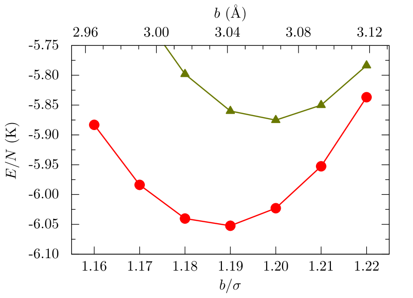
Figure 1: Variational energy (per particle) for the coordinated wavefunction given by Eqs. (2), (8)-(10) (bullets) and the Jastrow function with the McMillan pair factor given by Eq. (8) (triangles). Both energies are shown as a function of parameter $b$ which enters the two-body correlation factors. For each value of $b$, the coordinated function was optimized with respect to its parameters $m$ and $\delta$. For the unit of distance, we use $\sigma=2.556\,$Å. The energies were computed for 512-particle systems interacting with Aziz-IIAziz et al. (1987) pairwise potential. Statistical errors are smaller than the symbol size.

To test the coordinated wavefunction of Eq. (2), we have decided to limit the Jastrow term to the simple McMillan formMcMillan (1965) with $u_{2}=-(b/r)^{5}$. As this term aims to capture the short-range correlations in the fluid, the mid-range correlations are left to be treated with the coordination term. Having only one variational parameter in the Jastrow product simplifies the parametrization of the wavefunction. However, the simple form of the McMillan factor misses over 1 K of the correlation energy, most of it due to its imperfection at short distances. One should not hope to recover this energy with any improvement to the mid-range correlations.

For calculations, we used the following form of the pairwise functions,

$$u_{2}(r) =-\frac{1}{2}\left(\frac{b}{r}\right)^{5}-\frac{1}{2}\left(\frac{b}{2L_{c}-r}\right)^{5}+\left(\frac{b}{L_{c}}\right)^{5}$$ (8)

$$y_{2}(r) =1-\exp\left[-\left(\frac{\delta}{R(r)}\right)^{m}\right]$$ (9)

$$R(r) =\frac{r}{1-(r/L_{c})^{4}},$$ (10)

where $b$, $m$, and $\delta$ are the three variational parameters, and $L_{c}$ is the cutoff distance of the calculation given by half the dimension of the simulation box.

Table 1: Optimized parameters of the coordinated and non-coordinated Jastrow wavefunctions with the McMillan factor. Distances are specified in units of $\sigma=2.556$Å. Lowest line shows the thermodynamic limit extrapolation of the per-particle energy, with up to 1920 particles used for the calculation. The interaction was modeled with the Aziz pair potential from Ref. Aziz et al., 1987.

		Coordinated		Non-coord.
$b/\sigma$		$1.19$		$1.20$
$\delta/\sigma$		$1.60$		—
$m$		$6.55$		—
$E/N$ (K)		$-6.05(1)$		$-5.88(1)$

The coordination function $y_{2}$ was chosen to provide a reasonably sharp cutoff beyond a certain distance $\delta$. At the same time, we found it quite important to have a “flat” $y_{2}$ at small distances, as otherwise the derivative of $y_{2}$ interferes with the energy terms produced by the derivatives of the pair factors $u_{2}$. Because of this effect , using $y_{2}$ of a Gaussian or exponential form results in wide flat energy plateaus in the space of variational parameters. Instead, the form given by Eq. (9) assures that $y_{2}$ reaches a constant at small distances. The relevant small distances are given by the parameter $b$, and the condition can be formulated as

$$\exp[-(\delta/b)^{m}]\ll 1.$$

Satisfying the above condition effectively decouples the optimization of $u_{2}$ and $y_{2}$, allowing for a clear interpretation of both terms and for a straight-forward variational optimization. Indeed, we found that variationally optimized parameters $b,\delta$ and $m$ fulfill the above condition to about $10^{-3}$.

As is beneficial for a variational calculation, both Jastrow and the coordination terms are symmetrized to result in zero gradient of the wavefunction at the computational cutoff $L_{c}$. The pair term in Eq. (8) is symmetrized in the traditional manner, while the coordination factor $y_{2}$ employs a scaling function $R(r)$ to assure that $y_{2}$ vanishes smoothly at the cutoff distance $r=L_{c}$. The use of the scaling function allows for a robust implementation of the cutoffat $L_{c}$, yet introduces minimal disturbance to $y_{2}$ at the relevant distances $r\approx\delta$, as in our case $(\delta/L_{c})^{4}<10^{-2}$. We found that using scaling function provides a convenient way for symmetrizing the wavefunction.

III Results

III.1 Variational optimization

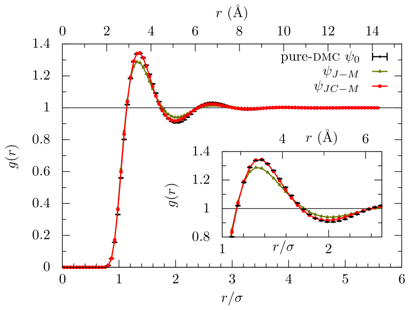
Figure 2: Pair distribution function $g(r)$ as a function of the interparticle distance, obtained for a 512-atom system. For the unit of distance, we use $\sigma=2.556\,$Å. Unconnected black errors bars: unbiased (pure) estimator obtained with DMC, as described in the text. Connected green triangles: Jastrow function with the McMillan pair factor as specified in Eq. (8). Connected red bullets: energy-optimized three-parameter coordinated wavefunction $\psi_{JC}$ with the McMillan factor, given by Eqs. (2),(8)-(10). Errors bars for both VMC calculations are smaller than their corresponding symbol sizes. The inset shows the details of the first correlation peak.

We carried the variational optimization with three-dimensional 512-atom ⁴He system at the equilibrium densityOuboter and Yang (1987) of liquid ⁴He, $\rho_{0}=0.365\sigma^{-3}=21.8~{}\text{nm}^{-3}$. Here and below, we use the reduced unit of length equal to $\sigma=2.556\,\text{\AA}$. All observables where computed on Markov chains generated by the Metropolis method Metropolis and Ulam (1949) with single-particle updates. We used a GPU cluster to speed up the calculations using a modification of the QL quantum Monte Carlo package Lutsyshyn (2015). The coordinated wavefunction of Eq. (2) was taken in three-parameters form given by Eqs. (8–10). The system Hamiltonian

$$\hat{H}=-\frac{\hbar^{2}}{2m}\sum_{i}\nabla^{2}_{i}+\sum_{i<j}V(r_{ij})$$

was used with the pair potential by AzizAziz et al. (1987).

The three variational parameters $b$, $m$, and $\delta$ were optimized on a grid. Figure 1 shows variational energy as a function of parameter $b$, given optimal $m$ and $\delta$ for each value of $b$. The results are compared to the (non-coordinated) Jastrow function with the McMillan factor given by Eq. (8). Optimal value of the parameter $b$ for for the coordinated function was found to be $b=1.19\sigma$, slightly below the optimal value of the non-coordinated function, $b=1.20\sigma$. As expected, we found little variation in optimal value of $\delta$ with respect to changing the value of parameter $b$. In the range shown in Figure 1, optimal $\delta$ varies less than two percent. We also notice relatively weak correlation between parameters $\delta$ and $m$ near the variational minimum.

The optimized values of variational parameters are shown in Table 1. The table also shows the value of optimized energy extrapolated to the thermodynamic limit. For comparison, Table 1 also lists the energy for the Jastrow function with the McMillan factor. This energy differs slightly from the one obtained by McMillanMcMillan (1965), which can be prescribed to the difference in the interaction potential. As expected, one will notice that the gain in the correlation energy is mild, and amounts to just under 200 mK. This is in part due to the fact that the missing mid-range correlations are not responsible for a large amount of energy, but also because the presence of the coordination term ever so slightly offsets the correlation hole which in turn carries an energy penalty.

III.2 Structural properties of the coordinated function

Table 2: The degree to which the computed pair distribution functions $g(r)$ capture the unbiased estimate $g^{*}(r)$. The values are computed as $|g(r_{m})-g^{*}(r_{m})|/|1-g^{*}(r_{m})|$, where $r_{m}$ are the locations of extrema of $g^{*}(r)$. The simulation conditions are described in Figure 2.

		$1^{\text{st}}\max$	$1^{\text{st}}\min$	$2^{\text{nd}}\max$	$2^{\text{nd}}\min$	$3^{\text{rd}}\max$	$3^{\text{rd}}\min$
Coordinated		$1.0$	$0.9$	$0.7$	$0.6$	$0.4$	$0.4$
Non-coor.		$0.8$	$0.6$	$0.5$	$0.3$	$0.2$	$0.2$

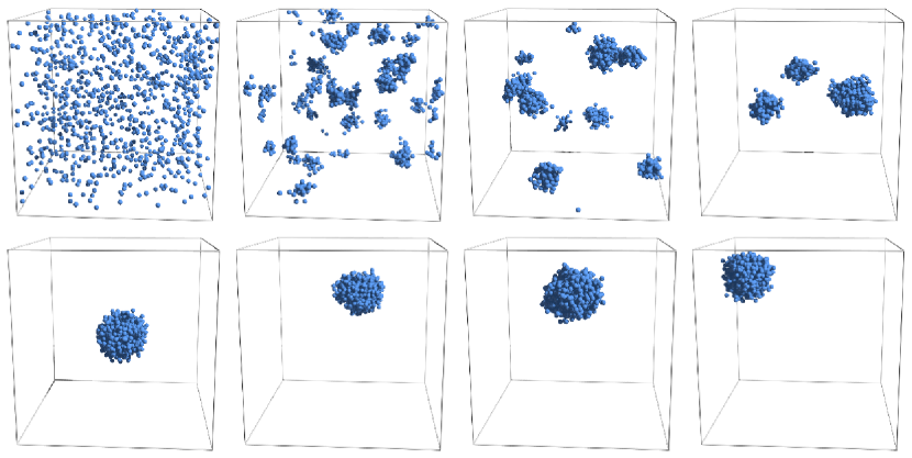
Figure 3: Progression of Markov chain during Metropolis sampling of a system with $N=1000$ atoms with the coordinated wavefunction. The size of the cubic box is equal to $L=100\,\sigma=256\,\text{\AA}$, which would correspond to a very dilute homogeneous system. Top row, left to right, shows the initial state of the system (with atoms distributed randomly and uniformly), and the system correspondingly after $10^{3}$, $10^{4}$, and $10^{5}$ macroupdates. After $10^{5}$ updates, the Markov chain reaches droplet configuration which is then sampled throughout the (periodic) simulation cell. The bottom row, left to right, shows configurations after $2\cdot 10^{5}$, $3\cdot 10^{5}$, $10^{6}$, and $2\cdot 10^{6}$ macroupdates. Wavefunction parameters $b=1.19\,\sigma$, $\delta=4.60\,\sigma$, $m=6.55$. Metropolis sampling was carried via single-particle updates, with a fixed Gaussian-distribution of displacements which resulted in the acceptance ratio of above 20% in the homogeneous phase to below 35% in the condensed phase. Each “macroupdate” equals $N$ single-particle Metropolis attempts.

As both the potential energy and the wavefunction are built from the pairwise functions, the properties of the system are captured by the pair distribution function. The computed pair distribution function $g(r)$ is shown in Figure 2, along with the results for the McMillan function and an unbiased (pure) estimate for the $g(r)$ obtained with the diffusion Monte Carlo (DMC). The unbiased DMC estimator for $g(r)$ was obtained with the ancestry tracking algorithm of Casulleras and Boronat Casulleras and Boronat (1995). Such an unbiased estimator is computed from the projected ground state and can be expected to reflect accurately on the experimental values Barnett et al. (1991); Casulleras and Boronat (1995); Marin et al. (2005). In properly converged calculations, pure DMC results do not depend on the DMC guiding function. However, it is worth pointing out that the guiding function for the DMC calculation was in fact the Jastrow function with the McMillan factor and it did not contain the coordination factor. In all three cases shown in Figure 2, the calculations were performed with 512-particle systems at the equilibrium density of ⁴He, $\rho=0.365\sigma=21.8\text{ nm}^{-3}$. The variational parameters were chosen by energy optimization, as specified above, and are given in Table 1.

It is notable that the coordinated wavefunction reproduces accurately the first correlation peak in the pair distribution function. The inset in Figure 2 shows the detail of the first maximum. The first correlation minimum is reproduced slightly less accurately. The following oscillations in the pair distribution function are also reproduced better by the coordinated wavefunction, albeit with decreasing accuracy. The position of the maxima and minima in the pair distribution was also considerably improved by the coordination term. The details are given in Table 2. However, the absolute value of these successive oscillations is minute, and they are at distances where the pair potential is vanishing rapidly. Thus their influence to the overall energy is nonsignificant.

IV Inhomogeneous systems

Jastrow wavefunctions based on a short-range pair factors cannot support the formation of a self-bound state. That is, a simulation in a sufficiently large box will result in a low-density uniform gas with near-zero potential and kinetic energy. Helium liquid, however, is self-bound. To describe inhomogeneous systems, one generally adds one-body factors which bind the liquid phase to a desired shape Valles and Schmidt (1988); Liu et al. (1975); Marin et al. (2005); Epstein and Krotscheck (1988). This has obvious disadvantages if the surface shape is complex, and may pose additional challenges when one needs to maintain the translational symmetry in the system Lutsyshyn and Halley (2011). Parametrization of the surface adds to the required number of the variational variables. Self-binding may also be enforced through the use of long-range terms in the two-body factors, such as introduced in Ref. Navarro et al., 2012, with additional term in two-body function $u_{2}(r)$ proportional to the distance between the particles $r$. Such a wavefunction serves well as a trial wavefunction for a projector Monte Carlo calculation, yet variationally, kinetic per-particle energy of a system with $u_{2}\sim-\alpha r$ for large $r$ is divergent with the increasing number of particles $N$ as $\sim(\hbar^{2}/m)\rho_{0}^{1/3}N^{2/3}\alpha$, where $\rho_{0}$ is the bulk density. This presents a number of challenges, as at the very least $\alpha$ must be $N$-dependent.

The coordinated wavefunction has an unexpected feature in that by design it supports a self-bound state of the atoms. Upon inspection, one will notice that the coordination sum-factors in Eq. (2) in fact vanish in the limit of low-density, uniformly distributed gas. Thus the coordination term requires that atoms form clusters, so far as function $y_{2}(r)$ falls off sufficiently rapidly with distance. The size and number of the clusters is determined by the variational parameters and particle density. For instance, a gas of dimers already has non-zero coordination term. Increasing the range of $y_{2}$ (which in our case translates to increasing $\delta$ or decreasing $m$) increases the size of the clusters. The parameters also provide control over the structure of the surface.

We have carried variational calculation with the coordinated wavefunction with 1000 atoms in a simulation box that resulted in particle density $10^{-3}\,\sigma^{-3}\approx 0.06\,\text{~{}nm}^{-3}$. The Jastrow wavefunction results in a ground state of dilute gas with close to zero energy. However, the coordinated wavefunction resulted in a bound state for a wide range of parameters $m$ and $\delta$. Only small $\delta$ resulted in the unbound states albeit with positive energy. We also find that the extent of function $y_{2}$ controls the average cluster size and thus the energy. Variational optimization of $m$ and $\delta$ results in a state with a single liquid droplet.

To demonstrate the robustness of the inhomogeneous simulation, we carried Monte Carlo sampling of the coordinated wavefunction with parameters $m=6.55$ and $\delta=4.50\,\sigma$ (i.e., with $y_{2}$ having larger extent than for the bulk). The initial coordinates of the 1000 particles were randomly distributed in the simulation box. The sampling sequence is presented in Figure 3. Soon after the start, the Markov chain arrives at configurations with multiple small clusters. As the clusters merge, a single droplet is eventually formed. The center of mass of the system is not fixed, and the droplet continues to sample the entire simulation cell.

The inner structure of the droplets and clusters depend strongly on the two-body function $u_{2}$. However, Jastrow function with the McMillan factor underestimates the equilibrium density of the bulk ⁴He. Without the fixed density constraint, it is to be expected that the inhomogeneous simulation should result in lower densities of the condensed phase. This was indeed observed. For example, the droplet shown in Figure 3 has inner density that is less than 70% of the bulk equilibrium helium density. Thus the droplet calculation presented here should be seen as a demonstration of principle. The details of their structure, which require a more detailed Jastrow term, will be the subject of further investigation.

V Conclusion

We have considered a wavefunction ansatz for strongly correlated Bose system that goes beyond the Jastrow-Feenberg expansion. Originating from a symmetrical solid wavefunction proposed by Cazorla et al. Cazorla et al. (2009), it is a Bose-liquid wavefunction which explicitly promotes the creation of the coordination shells around atoms. The function is translationally and exchange symmetric. It is fully explicit and is computationally hard as $O(N^{2})$, making it well suitable for treatment with quantum Monte Carlo.

To demonstrate the coordination effect, we have studied the wavefunction with the one-parameter McMillan factor for the Jastrow term, and a two-parameter coordination function. The resulting three-parameter wavefunction was straight-forward to optimize variationally. The short-range nature of the McMillan factor allowed to directly observe the effects of the coordination terms on the mid-range structure of the liquid. Indeed, the optimized wavefunction results in superior description of mid-range correlations in the system. Comparing with unbiased estimate for the pair distribution function obtained with the diffusion Monte Carlo, we find that the first correlation peak is reproduced almost exactly. Moreover, the structure of the pair distribution function is improved consistently throughout larger distances as well.

As was first demonstrated in Ref. Michelis and Reatto, 1974, the first correlation peak can be reproduced rather exactly with the Jastrow function. However, this required eight variational parameters, and already the description of the first minimum was significantly lacking. Other approaches to accurately describe the mid-range structure with the Jastrow factors alone have also been reported Chin (1996). In our case, the addition of the coordination term allows to separate the short- and middle-range correlations, which can be accounted for correspondingly by the Jastrow and the coordination terms.

By construction, the coordinated wavefunction supports a self-bound state. Consequently, the simulation of inhomogeneous systems does not require the addition of one-body terms. Moreover, inhomogenuity and surface formation at low densities result directly from the variational optimization of the bulk wavefunction. Since the variational ansatz does not require knowledge of the surface geometry, this also provides a powerful tool for cluster states of matter. However, we find that a satisfactory description of the inhomogeneous phase of helium requires improvements in the Jastrow pair term, which was here limited to the McMillan form for simplicity.

The separation of the mid-range correlations into the coordination term which was demonstrated here means that the Jastrow pair term in the coordinated wavefunction only needs to account for the short-range correlations and possibly for the well-understood long-range correlations arising from zero-point phonons. This makes it promising that an accurate short-range pair term can be designed in future with a simple parametrization.

References

- Bishop et al. (2000) R. F. Bishop, K. A. Gernoth, and N. R. Walet, eds., 150 Years of Quantum Many-Body Theory (World Scientific Publishing Co., Singapore, 2000).
- Vassen et al. (2012) W. Vassen, C. Cohen-Tannoudji, M. Leduc, D. Boiron, C. I. Westbrook, A. Truscott, K. Baldwin, G. Birkl, P. Cancio, and M. Trippenbach, Rev. Mod. Phys. 84, 175 (2012).
- Ketterle (2002) W. Ketterle, Rev. Mod. Phys. 74, 1131 (2002).
- Greywall (1993) D. S. Greywall, Phys. Rev. B 47, 309 (1993).
- Nakashima et al. (2011) Y. Nakashima, T. Matsushita, M. Hieda, N. Wada, H. Nishihara, and T. Kyotani, J. Low Temp. Phys. 162, 565 (2011).
- Anderson (1980) J. B. Anderson, J. Chem. Phys. 73, 3897 (1980).
- Ceperley and Alder (1980) D. M. Ceperley and B. J. Alder, Phys. Rev. Lett. 45, 566 (1980).
- Sarsa et al. (2000) A. Sarsa, K. E. Schmidt, and W. R. Magro, J. Chem. Phys. 113, 1366 (2000).
- Galli and Reatto (2003) D. Galli and L. Reatto, Mol. Phys. 101, 1697 (2003).
- Cuervo et al. (2005) J. Cuervo, P. Roy, and M. Boninsegni, J. Chem. Phys. 122, 114504 (2005).
- Rota et al. (2010) R. Rota, J. Casulleras, F. Mazzanti, and J. Boronat, Phys. Rev. E 81 (2010).
- Feenberg (1974) E. Feenberg, Ann. Phys. 84, 128 (1974).
- Chang and Campbell (1977) C. C. Chang and C. E. Campbell, Phys. Rev. B 15, 4238 (1977).
- Bijl (1940) A. Bijl, Physica, 7, 869 (1940).
- Jastrow (1955) R. Jastrow, Phys. Rev. 98, 1479 (1955).
- McMillan (1965) W. L. McMillan, Phys. Rev. 138, A442 (1965).
- Schiff and Verlet (1967) D. Schiff and L. Verlet, Phys. Rev. 160, 208 (1967).
- Vranješ et al. (2005) L. Vranješ, J. Boronat, J. Casulleras, and C. Cazorla, Phys. Rev. Lett. 95, 145302 (2005).
- Cazorla et al. (2012) C. Cazorla, Y. Lutsyshyn, and J. Boronat, Phys. Rev. B 85, 024101 (2012).
- Michelis and Reatto (1974) C. D. Michelis and L. Reatto, Phys. Lett. A 50, 275 (1974).
- Reatto (1979) L. Reatto, Nucl. Phys. A 328, 253 (1979).
- Reatto and Chester (1967) L. Reatto and G. V. Chester, Phys. Rev. 155, 88 (1967).
- Francis et al. (1970) W. P. Francis, G. V. Chester, and L. Reatto, Phys. Rev. A 1, 86 (1970).
- Masserini and Reatto (1984) G. L. Masserini and L. Reatto, Phys. Rev. B 30, 5367 (1984).
- Masserini and Reatto (1987) G. L. Masserini and L. Reatto, Phys. Rev. B 35, 6756 (1987).
- Vitiello and Schmidt (1992) S. A. Vitiello and K. E. Schmidt, Phys. Rev. B 46, 5442 (1992).
- Vitiello and Schmidt (1999) S. A. Vitiello and K. E. Schmidt, Phys. Rev. B 60, 12342 (1999).
- Note (1) A prominent exception, the Feynman-Cohen backflow wavefunction Feynman and Cohen (1956), is in fact not designed for a ground state of bosonic many-body system, but is instead commonly used for the excited states of 4He Feynman and Cohen (1956); Galli et al. (2014); Vranješ et al. (2005) and for the fermionic systems Panoff and Carlson (1989); Kwon et al. (1993); Arias de Saavedra et al. (2012); Drummond and Needs (2013); Motta et al. (2015).
- Vitiello et al. (1988) S. Vitiello, K. Runge, and M. H. Kalos, Phys. Rev. Lett. 60, 1970 (1988).
- Reatto and Masserini (1988) L. Reatto and G. L. Masserini, Phys. Rev. B 38, 4516 (1988).
- MacFarland et al. (1992) T. MacFarland, S. Vitiello, and L. Reatto, J. Low Temp. Phys. 89, 433 (1992).
- MacFarland et al. (1994) T. MacFarland, S. A. Vitiello, L. Reatto, G. V. Chester, and M. H. Kalos, Phys. Rev. B 50, 13577 (1994).
- Zhang et al. (1994) S. Zhang, M. Kalos, G. Chester, S. Vitiello, and L. Reatto, Phys. B: Cond. Mat. 194–196, 523 (1994).
- Cazorla et al. (2009) C. Cazorla, G. E. Astrakharchik, J. Casulleras, and J. Boronat, New J. Phys. 11, 013047 (2009).
- Lutsyshyn et al. (2014) Y. Lutsyshyn, G. E. Astrakharchik, C. Cazorla, and J. Boronat, Phys. Rev. B 90, 214512 (2014).
- Lutsyshyn et al. (2010a) Y. Lutsyshyn, C. Cazorla, and J. Boronat, J. Low Temp. Phys. 158, 608 (2010a).
- Lutsyshyn et al. (2011) Y. Lutsyshyn, R. Rota, and J. Boronat, J. Low Temp. Phys. 162, 455 (2011).
- Lutsyshyn et al. (2010b) Y. Lutsyshyn, C. Cazorla, G. E. Astrakharchik, and J. Boronat, Phys. Rev. B 82, 180506 (2010b).
- Cazorla et al. (2013) C. Cazorla, Y. Lutsyshyn, and J. Boronat, Phys. Rev. B 87, 214522 (2013).
- Fabrocini et al. (2002) A. Fabrocini, S. Fantoni, and E. Krotscheck, eds., Introduction to Modern Methods of Quantum Many-body Theory and Their Applications (2002).
- Note (2) Notice that the term in non-linear; contributions from the Jastrow term have to be added before squaring the vector.
- Aziz et al. (1987) R. A. Aziz, F. R. W. McCourt, and C. C. K. Wong, Mol. Phys. 61, 1487 (1987).
- Ouboter and Yang (1987) R. D. B. Ouboter and C. N. Yang, Physica 144, 127 (1987).
- Metropolis and Ulam (1949) N. Metropolis and S. Ulam, J. Am. Statist. Assoc. 44, 335, (1949).
- Lutsyshyn (2015) Y. Lutsyshyn, Comp. Phys. Comm. 187, 162 (2015).
- Casulleras and Boronat (1995) J. Casulleras and J. Boronat, Phys. Rev. B 52, 3654 (1995).
- Barnett et al. (1991) R. N. Barnett, P. J. Reynolds, and W. A. Lester Jr, J. Comp. Phys. 96, 258 (1991).
- Marin et al. (2005) J. M. Marin, J. Boronat, and J. Casulleras, Phys. Rev. B 71, 144518 (2005).
- Valles and Schmidt (1988) J. L. Valles and K. E. Schmidt, Phys. Rev. B 38, 2879 (1988).
- Liu et al. (1975) K. S. Liu, M. H. Kalos, and G. V. Chester, Phys. Rev. B 12, 1715 (1975).
- Epstein and Krotscheck (1988) J. L. Epstein and E. Krotscheck, Phys. Rev. B 37, 1666 (1988).
- Lutsyshyn and Halley (2011) Y. Lutsyshyn and J. W. Halley, Phys. Rev. B 83, 014504 (2011).
- Navarro et al. (2012) J. Navarro, D. Mateo, M. Barranco, and A. Sarsa, J. Chem. Phys. 136, 054301 (2012).
- Chin (1996) S. A. Chin, “A new Jastrow wavefunction for simulating liquid helium,” (1996), unpublished.
- Feynman and Cohen (1956) R. P. Feynman and M. Cohen, Phys. Rev. 102, 1189 (1956).
- Galli et al. (2014) D. E. Galli, L. Reatto, and M. Rossi, Phys. Rev. B 89, 224516 (2014).
- Panoff and Carlson (1989) R. M. Panoff and J. Carlson, Phys. Rev. Lett. 62, 1130 (1989).
- Kwon et al. (1993) Y. Kwon, D. M. Ceperley, and R. M. Martin, Phys. Rev. B 48, 12037 (1993).
- Arias de Saavedra et al. (2012) F. Arias de Saavedra, F. Mazzanti, J. Boronat, and A. Polls, Phys. Rev. A 85, 033615 (2012).
- Drummond and Needs (2013) N. D. Drummond and R. J. Needs, Phys. Rev. B 88, 035133 (2013).
- Motta et al. (2015) M. Motta, G. Bertaina, D. Galli, and E. Vitali, Comp. Phys. Comm. 190, 62 (2015).