Stability of resonant configurations during the migration of planets and constraints on disk-planet interactions

We study the stability of mean-motion resonances (MMR) between two planets during their migration in a protoplanetary disk. We use an analytical model of resonances, and describe the effect of the disk by a migration timescale ($T_{m,i}$) and an eccentricity damping timescale ($T_{e,i}$) for each planet ($i=1,2$ respectively for the inner and outer planet). We show that the resonant configuration is stable if $T_{e,1}/T_{e,2}>(e_{1}/e_{2})^{2}$. This general result can be used to put constraints on specific models of disk-planet interactions. For instance, using classical prescriptions for type I migration, we show that when the angular momentum deficit (AMD) of the inner orbit is larger than the outer’s orbit AMD, resonant systems must have a locally inverted disk density profile to stay locked in resonance during the migration. This inversion is very untypical of type I migration and our criterion can thus provide an evidence against classical type I migration. That is indeed the case for the Jupiter-mass resonant systems HD~60532b, c (3:1 MMR), GJ~876b, c (2:1 MMR), and HD~45364b, c (3:2 MMR). This result may be an evidence for type II migration (gap opening planets), which is compatible with the large masses of these planets.

1 Introduction

In Delisle et al. (2014), we showed that tidal dissipation raised by the star on two resonant planets can produce three kinds of distinct evolutions depending on the relative strength of the dissipation in both planets. The three different outcomes of this tidal process are systems that stay in resonance, systems that leave the resonance with an increasing period ratio ($P_{out}/P_{in}$) and systems that leave the resonance with a decreasing period ratio. For known near resonant systems, the comparison of the period ratio of the planets with respect to the nominal resonant value helps to put constraints on the tidal dissipation undergone by each planet and thus on the nature of the planets (see Delisle et al., 2014). In this article, we generalize our reasoning to other forms of dissipation, in particular to disk-planet interactions.

Disk-planet interactions can induce migration of the planets (e.g. Goldreich & Tremaine, 1979). In the case of convergent migration (i.e. decreasing period ratio), the planets can be locked in resonance (e.g. Weidenschilling & Davis, 1985). Two planets that are locked in resonance have their eccentricities excited on the migration timescale (e.g. Weidenschilling & Davis, 1985). However, disk-planet interactions also induce exponential eccentricity damping. Depending on the respective timescales of the migration and eccentricity damping, the system can reach a stationary state in which eccentricities stay constant (Lee & Peale, 2002). The semi-major axes continue to evolve but the semi-major axis ratio (or period ratio) stays locked at the resonant value. Recently, Goldreich & Schlichting (2014) showed that this equilibrium is unstable in the case of the circular restricted three body problem where the inner planet has negligible mass. This means that after the resonance locking, the eccentricity of the inner planet reach an equilibrium value but then undergoes larger and larger oscillations around this equilibrium value until the system reaches the resonance separatrix and leaves the resonance. Then, the period ratio is no more locked at the resonant value and the convergent migration continues (decreasing period ratio) until the system reaches another resonance. The timescale of the resonance escape is given by the eccentricity damping timescale and is thus short compared to the migration timescale (see Goldreich & Schlichting, 2014). Therefore, Goldreich & Schlichting (2014) concluded that when the disk disappears and the migration stops, only a few systems should be observed in resonance. However, this conclusion is mainly based on a particular case in which the mass of the inner planet is much smaller than the mass of the outer planet whose eccentricity is negligible and the migration and damping forces are only undergone by the inner planet. As shown in Delisle et al. (2014), the evolution of a resonant system under dissipation highly depends on which planet is affected by the dissipation. In this paper we study a more general case in which both planets have masses, eccentricities, and undergo dissipative forces.

In Sect. 2 we introduce the notations and the model of the resonant motion in the conservative case that we developed in Delisle et al. (2014). In Sect. 3 we study the dissipative evolution of resonant planets in a very general framework (Sect. 3.1), and we apply this modeling to disk-planet interactions (Sect. 3.2). In Sect. 4 we show how our model can be used to put constraints on disks properties for observed resonant systems. In Sect. 5 we apply these analytical constraints to selected examples, and compare them with numerical simulations. We specifically study HD~60532b, c (3:1 resonance, Sect. 5.1) GJ~876b, c (2:1 resonance, Sect. 5.2), and HD~45364b, c (3:2 resonance, Sect. 5.3).

2 Resonant motion in the conservative case

In the following, we refer to the star as body 0, to the inner planet as body 1, and to the outer planet as body 2. We note $m_{i}$ the masses of the three bodies, and introduce $\mu_{i}=\mathcal{G}(m_{0}+m_{i})$ and $\beta_{i}=m_{0}m_{i}/(m_{0}+m_{i})$, where $\mathcal{G}$ is the gravitational constant. We only consider the planar case in this study.

In Delisle et al. (2014) we constructed a simplified, and integrable model of the resonant motion in the conservative and planar case. The main simplification of this model is to assume that the eccentricity ratio ($e_{1}/e_{2}$) stays close to the forced eccentricities ratio ($e_{1,ell}/e_{2,ell}$). These forced eccentricities correspond to the eccentricities at the elliptical fixed point at the resonance libration center. With this assumption, and assuming moderate eccentricities , the Hamiltonian of the system can be simplified (see Delisle et al., 2014) to the following simple pendulum Hamiltonian

$$\mathcal{H}=-\epsilon^{2}+2R\delta^{q/2}\cos(q\theta),$$ (1)

where $q$ is the degree of the resonance ($q=k_{2}-k_{1}$ for a $k_{2}$:$k_{1}$ resonance), $\epsilon$ is the action coordinate and provides a measure of the distance to the exact commensurability. $\theta$ is the unique resonant angle in this simplified model. It is a combination of both usual resonant angles ($\sigma_{i}=\frac{k_{2}}{q}\lambda_{2}-\frac{k_{1}}{q}\lambda_{1}-\varpi_{i}$, see Appendix B, Eqs. (97) and (99) and Delisle et al., 2014). $R$ is a constant that depends on the masses of the bodies and on the considered resonance (see Delisle et al., 2014). $\delta$ is a constant of motion (parameter of the model). We have

$$\epsilon = \Lambda_{1}-\Lambda_{1,0}+\Lambda_{2}-\Lambda_{2,0},$$ (2)

$$\delta = \Lambda_{1,0}-G_{1}+\Lambda_{2,0}-G_{2},$$ (3)

where $\Lambda_{i}$ is the renormalized circular angular momentum of planet $i$, $G_{i}$ its renormalized angular momentum (see Appendix A and Delisle et al., 2014). The subscript 0 denotes the values at the exact commensurability. The quantities $\Lambda_{i}$ only depend on the semi-major axis ratio $\alpha=a_{1}/a_{2}$

$$\Lambda_{1}(\alpha) = \frac{1}{(k_{2}/k_{1})+(\beta_{2}/\beta_{1})\sqrt{\mu_{2}/(\mu_{1}\alpha})}$$

$$\approx \frac{1}{(k_{2}/k_{1})+(m_{2}/m_{1})/\sqrt{\alpha}},$$

$$\Lambda_{2}(\alpha) = \frac{1}{1+(k_{2}/k_{1})(\beta_{1}/\beta_{2})\sqrt{\mu_{1}\alpha/\mu_{2}}}$$

$$\approx \frac{1}{1+(k_{2}/k_{1})(m_{1}/m_{2})\sqrt{\alpha}},$$

At the exact commensurability, we have

$$\alpha_{0}=\left(\frac{\mu_{2}}{\mu_{1}}\right)^{1/3}\left(\frac{k_{1}}{k_{2}}\right)^{2/3}\approx\left(\frac{k_{1}}{k_{2}}\right)^{2/3}$$ (6)

The quantities $G_{i}$ depend on $\alpha$ and on the planet eccentricities

$$G_{i}(\alpha,e_{i})=\Lambda_{i}(\alpha)\sqrt{1-e_{i}^{2}}.$$ (7)

Let us note $I_{i}$ the renormalized angular momentum deficit (AMD) of planet $i$ (Laskar, 1997, 2000)

$$I_{i}=\Lambda_{i}-G_{i}=\frac{1}{2}\Lambda_{i}\xi_{i}^{2}\propto e_{i}^{2},$$ (8)

with

$$\xi_{i}=\sqrt{2\left(1-\sqrt{1-e_{i}^{2}}\right)}\approx e_{i}.$$ (9)

The simplifying assumption introduced in Delisle et al. (2014) implies (see also Appendix B)

$$\frac{I_{2}}{I_{1}}=\frac{I_{2,ell}}{I_{1,ell}}\equiv\tan^{2}\phi,$$ (10)

where $\phi$ is a constant angle and $I_{i,ell}$ are values of the renormalized AMD at the center of the resonance (elliptical fixed point, see Delisle et al., 2014). We also note $\mathcal{D}$ the renormalized total AMD

$$\mathcal{D}=I_{1}+I_{2}=\delta+\epsilon.$$ (11)

The parameter $\delta$ corresponds to the renormalized total AMD at the exact commensurability ($\delta=\mathcal{D}_{0}$). Thus, for a resonant system, $\delta$ provides a measure of the planet eccentricities ($\delta\propto e^{2}$, see Eq. (8)). Figure 1 shows the phase space corresponding to Hamiltonian (1). The width of the resonant area is proportional to $\delta^{q/4}\propto e^{q/2}$ for a resonance of order $q$ (see Fig. 1). For a resonant system, in the regime of moderate eccentricities, a measure (between 0 and 1) of the relative amplitude of libration (amplitude of libration versus resonance width) is given by (see Delisle et al., 2014)

$$A=\sin^{2}\left(\frac{q\theta_{max}}{2}\right),$$ (12)

where $\theta_{max}$ is the maximum value reached by the resonant angle $\theta$ during a libration period (see Fig. 1).

Figure 1: Phase space of a resonance of order $q$ in the simplified pendulum-like approximation (Hamiltonian (1)). $\theta$ is the unique resonant angle and $\epsilon$ its conjugated action. The separatrix is highlighted in red. The amplitude $A$ (defined with $\theta_{max}$ see Eq. (12)) is 0 at the center of the resonance (elliptical fixed point) and 1 at the separatrix.

Note that our simplifying assumption (eccentricity ratio close to the forced eccentricities ratio) is well verified when the amplitude of libration is small ($A\ll 1$) and the system stays close to the elliptical fixed point. For high amplitude of libration ($A\sim 1$), the eccentricity ratio undergoes oscillations around the forced value and our model only provide a first approximation of the motion (see Delisle et al., 2014).

3 Resonant motion in the dissipative case

In this section we describe the evolution of a resonant system undergoing dissipation. The main parameters that have to be tracked during this evolution are the parameter $\delta$ which describes the evolution of the phase space (and of the eccentricities for resonant systems) and the relative amplitude $A$ which describes the spiraling of the trajectory with respect to the separatrix of the resonance.

3.1 General case

Let us consider a dissipative force acting on the semi-major axes and the eccentricities of both planets. We first consider a very general case and do not assume a particular form for this dissipation, except that it acts on a long timescale. The evolution of the system can be described by the three following timescales (which may depend on the eccentricities and semi-major axes of the planets): $(\xi_{1}/\dot{\xi}_{1})_{d}$, $(\xi_{2}/\dot{\xi}_{2})_{d}$, $(\alpha/\dot{\alpha})_{d}$. Note that, for sufficiently small eccentricities, we have $\xi_{i}\approx e_{i}$, and

$$\left.\frac{\dot{\xi}_{i}}{\xi_{i}}\right|_{d}\approx\left.\frac{\dot{e}_{i}}{e_{i}}\right|_{d}.$$ (13)

The evolution of the parameter $\delta$ that drives the evolution of the phase space (and of the eccentricities for resonant systems) is given by (see Appendix C)

$$\dot{\delta}|_{d} = 2\left(\cos^{2}\phi\left.\frac{\dot{\xi}_{1}}{\xi_{1}}\right|_{d}+\sin^{2}\phi\left.\frac{\dot{\xi}_{2}}{\xi_{2}}\right|_{d}\right)\mathcal{D}$$

$$+\frac{\Lambda_{2}-\sin^{2}\phi}{2}\left.\frac{\dot{\alpha}}{\alpha}\right|_{d}\mathcal{D}$$

$$+\frac{q}{k_{1}}\frac{\Lambda_{1}\Lambda_{2}}{2}\left.\frac{\dot{\alpha}}{\alpha}\right|_{d}.$$

For a resonant system, the evolution of the relative amplitude of libration reads (see Delisle et al., 2014, Appendix A)

$$<\dot{A}>=\frac{1}{2R\delta^{q/2}}\left(<\epsilon\dot{\epsilon}|_{d}>-\frac{q}{4\delta}<\epsilon^{2}\dot{\delta}|_{d}>\right),$$ (15)

with

$$\dot{\epsilon}|_{d}=-\frac{q}{k_{1}}\frac{\Lambda_{1}\Lambda_{2}}{2}\left.\frac{\dot{\alpha}}{\alpha}\right|_{d}.$$ (16)

3.2 Disk-planet interactions

Let us now apply Eqs. (3.1), (15) to the specific case of disk-planet interactions. Because of these interactions the planets undergo a torque that induces a modification in their orbital elements and subsequent migration in the disk (e.g. Goldreich & Tremaine, 1979, 1980). In particular, the angular momentum of each planet evolves on an exponential timescale $T_{m,i}$ due to this migration, while eccentricities evolve on an exponential timescale $T_{e,i}$ (e.g. Papaloizou & Larwood, 2000; Terquem & Papaloizou, 2007; Goldreich & Schlichting, 2014):

$$\left.\frac{\dot{\hat{G}}_{i}}{\hat{G}_{i}}\right|_{d} = -\frac{1}{T_{m,i}},$$ (17)

$$\left.\frac{\dot{e}_{i}}{e_{i}}\right|_{d} = -\frac{1}{T_{e,i}},$$ (18)

where $\hat{G}_{i}$ is the angular momentum of planet $i$. From these simple decay laws we can deduce the evolution of the parameters of interest for resonant systems ($\dot{\delta}$ and $\dot{A}$, see Sect. 3.1). We have

$$\left.\frac{\dot{\xi}_{i}}{\xi_{i}}\right|_{d}\approx\left.\frac{\dot{e}_{i}}{e_{i}}\right|_{d}=-\frac{1}{T_{e,i}},$$ (19)

$$\left.\frac{\dot{a}_{i}}{a_{i}}\right|_{d}=-\frac{2}{T_{m,i}}+2\frac{\xi_{i}^{2}}{1-\xi_{i}^{2}}\left.\frac{\dot{\xi}_{i}}{\xi_{i}}\right|_{d}\approx-\frac{2}{T_{m,i}}-2\frac{\xi_{i}^{2}}{T_{e,i}}.$$ (20)

The evolution of the semi-major axis ratio is thus governed by

$$\left.\frac{\dot{\alpha}}{\alpha}\right|_{d}=\frac{2}{T_{m}}+\frac{4}{\Lambda_{1}\Lambda_{2}}\left(\frac{\Lambda_{1}\sin^{2}\phi}{T_{e,2}}-\frac{\Lambda_{2}\cos^{2}\phi}{T_{e,1}}\right)\mathcal{D},$$ (21)

with

$$\frac{1}{T_{m}}=\frac{1}{T_{m,2}}-\frac{1}{T_{m,1}}.$$ (22)

From Eq. (3.1) we obtain

$$\dot{\delta}|_{d} = \frac{q}{k_{1}}\frac{\Lambda_{1}\Lambda_{2}}{T_{m}}$$

$$+\frac{\Lambda_{2}-\sin^{2}\phi}{T_{m}}\mathcal{D}$$

$$-2\left(\frac{\cos^{2}\phi}{T_{e,1}}+\frac{\sin^{2}\phi}{T_{e,2}}\right)\mathcal{D}$$

$$+2\frac{q}{k_{1}}\left(\frac{\Lambda_{1}\sin^{2}\phi}{T_{e,2}}-\frac{\Lambda_{1}\cos^{2}\phi}{T_{e,1}}\right)\mathcal{D}$$

$$= \frac{q}{k_{1}}\frac{\Lambda_{1}\Lambda_{2}}{T_{m}}$$

$$-\mathcal{D}\left[2(\Lambda_{1}+\Lambda_{2})\left(\frac{k_{2}}{k_{1}}\frac{\cos^{2}\phi}{T_{e,1}}+\frac{\sin^{2}\phi}{T_{e,2}}\right)\right.$$

$$\qquad\left.-\frac{\Lambda_{2}-\sin^{2}\phi}{T_{m}}\right],$$

where we neglect second order terms in $\mathcal{D}$ ($\mathcal{D}^{2}\propto e^{4}$). Let us note

$$\frac{1}{T_{M}} = \frac{q}{k_{1}}\frac{\Lambda_{1}\Lambda_{2}}{T_{m}},$$ (24)

$$\frac{1}{T_{E}} = 2(\Lambda_{1}+\Lambda_{2})\left(\frac{k_{2}}{k_{1}}\frac{\cos^{2}\phi}{T_{e,1}}+\frac{\sin^{2}\phi}{T_{e,2}}\right)-\frac{\Lambda_{2}-\sin^{2}\phi}{T_{m}}.$$ (25)

We thus have

$$\dot{\delta}|_{d} = \frac{1}{T_{M}}-\frac{\mathcal{D}}{T_{E}},$$ (26)

$$<\dot{\delta}|_{d}> = \frac{1}{T_{M}}-\frac{\delta}{T_{E}}.$$ (27)

Note that the damping timescale is often much shorter than the migration timescale ($T_{e,i}\ll T_{m,i}$, e.g. Goldreich & Tremaine, 1980), thus

$$\frac{1}{T_{E}}\approx 2(\Lambda_{1}+\Lambda_{2})\left(\frac{k_{2}}{k_{1}}\frac{\cos^{2}\phi}{T_{e,1}}+\frac{\sin^{2}\phi}{T_{e,2}}\right).$$ (28)

The timescales $T_{E}$, $T_{M}$ can be expressed using more usual notations

$$\frac{1}{T_{M}} \approx \frac{q}{k_{1}}\left(2\frac{k_{2}}{k_{1}}+\frac{m_{2}}{m_{1}}\frac{1}{\sqrt{\alpha_{0}}}+\left(\frac{k_{1}}{k_{2}}\right)^{2}\frac{m_{1}}{m_{2}}\sqrt{\alpha_{0}}\right)^{-1}\times$$

$$\left(\frac{1}{T_{m,2}}-\frac{1}{T_{m,1}}\right),$$

$$\frac{1}{T_{E}} \approx 2\left(1+\frac{m_{1}}{m_{2}}\sqrt{\alpha_{0}}\right)\left(1+\frac{k_{2}}{k_{1}}\frac{m_{1}}{m_{2}}\sqrt{\alpha_{0}}\right)^{-1}\times$$

$$\left(\frac{1}{T_{e,2}}+\frac{k_{2}}{k_{1}}\frac{m_{1}}{m_{2}}\left(\frac{e_{1}}{e_{2}}\right)_{ell}^{2}\sqrt{\alpha_{0}}\frac{1}{T_{e,1}}\right)\left(1+\frac{m_{1}}{m_{2}}\left(\frac{e_{1}}{e_{2}}\right)_{ell}^{2}\sqrt{\alpha_{0}}\right)^{-1}.$$

Depending on the values of $T_{M}$ and $T_{E}$, different evolution scenarios for $\delta$ are possible. Note that all these equations remain valid for $T_{M}$ and $T_{E}$ negative. In most cases the disk induces a damping of eccentricities ($T_{e,i}>0$, thus $T_{E}>0$), but some studies (e.g. Goldreich & Sari, 2003) suggest that an excitation of the eccentricities by the disk is possible ($T_{e,i}<0$, thus $T_{E}<0$). $T_{M}$ is positive if the period ratio between the planets ($P_{2}/P_{1}$) decreases (convergent migration). But if the planets undergo divergent migration ($P_{2}/P_{1}$ increases), $T_{M}$ is negative. This does not depends on the absolute direction (inward or outward) of the migration of the planets in the disk but only on the evolution of their period ratio.

In the case of divergent migration, the planets cannot get trapped in resonance (e.g. Henrard & Lemaitre, 1983). The system always ends-up with a period ratio higher than the resonant value and this does not depend on the damping/excitation of eccentricities.

The case of convergent migration is more interesting. If the initial period ratio is higher than the resonant value, the planets can be locked in resonance. This induces an excitation of the eccentricities of the planets ($\dot{\delta}|_{M}=1/T_{M}>0$). If $T_{E}<0$ (excitation of eccentricities by the disk) or $T_{E}\gg T_{M}$ (inefficient damping), $\delta$ (as well as the eccentricities) does not stop increasing. When eccentricities reach too high values, the system becomes unstable and the resonant configuration is broken.

The most common scenario is the case of efficient damping of eccentricities ($0<T_{E}\lesssim T_{M}$). In this case, $\delta$ reaches an equilibrium value ($<\dot{\delta}|_{d}>=0$, see Eq. (27))

$$\delta_{eq} = \frac{T_{E}}{T_{M}}$$

$$= \frac{q}{2k_{1}}\frac{\Lambda_{1}\Lambda_{2}}{\Lambda_{1}+\Lambda_{2}}\left(\frac{1}{T_{m,2}}-\frac{1}{T_{m,1}}\right)\left(\frac{k_{2}}{k_{1}}\frac{\cos^{2}\phi}{T_{e,1}}+\frac{\sin^{2}\phi}{T_{e,2}}\right)^{-1}$$

$$\approx \frac{q}{2}\left(1+\frac{m_{1}}{m_{2}}\left(\frac{e_{1}}{e_{2}}\right)_{ell}^{2}\sqrt{\alpha_{0}}\right)\times$$

$$\left(k_{1}+k_{2}+k_{2}\frac{m_{1}}{m_{2}}\sqrt{\alpha_{0}}+k_{1}\frac{m_{2}}{m_{1}}\frac{1}{\sqrt{\alpha_{0}}}\right)^{-1}\times$$

$$\left(\frac{1}{T_{m,2}}-\frac{1}{T_{m,1}}\right)\left(\frac{1}{T_{e,2}}+\frac{k_{2}}{k_{1}}\frac{m_{1}}{m_{2}}\left(\frac{e_{1}}{e_{2}}\right)_{ell}^{2}\sqrt{\alpha_{0}}\frac{1}{T_{e,1}}\right)^{-1}.$$

However, as shown by Goldreich & Schlichting (2014) for the restricted three body problem, this equilibrium can be unstable. Even if the parameter $\delta$ reaches the equilibrium $\delta_{eq}$ and the phase space of the system stops evolving, the amplitude of libration can increase until the system crosses the separatrix and escapes from resonance.

Let us now compute the evolution of this amplitude of libration. According to Eq. (15), we need to compute $<\epsilon\dot{\epsilon}|_{d}>$ and $<\epsilon^{2}\dot{\delta}|_{d}>$. We have

$$<\epsilon\dot{\epsilon}|_{d}> = 2\frac{q}{k_{1}}\left(\frac{\Lambda_{2}\cos^{2}\phi}{T_{e,1}}-\frac{\Lambda_{1}\sin^{2}\phi}{T_{e,2}}\right)<\epsilon^{2}>,$$ (32)

$$<\epsilon^{2}\dot{\delta}|_{d}> = \left(\frac{1}{T_{M}}-\frac{\delta}{T_{E}}\right)<\epsilon^{2}>=<\dot{\delta}|_{d}><\epsilon^{2}>,$$ (33)

where $<\epsilon^{2}>$ can be computed using elliptic integrals (see Delisle et al., 2014)

$$<\epsilon^{2}>\approx 2R\delta^{q/2}A.$$ (34)

Note that the first term ($<\epsilon\dot{\epsilon}|_{d}>$) does not depend on the migration timescale but only on the damping timescale. The second term ($<\epsilon^{2}\dot{\delta}|_{d}>$) vanishes when the system reaches the equilibrium $\delta=\delta_{eq}$, since $\dot{\delta}|_{d}=0$. This is not surprising because the first term describes the evolution of the absolute amplitude of libration $\epsilon^{2}$, while the second one describes the evolution of the resonance width which does not evolve if the phase space does not evolve (constant $\delta$). Finally, we obtain (see Eq. (15))

$$\left.\frac{\dot{A}}{A}\right|_{d}=2\frac{q}{k_{1}}\left(\frac{\Lambda_{2}\cos^{2}\phi}{T_{e,1}}-\frac{\Lambda_{1}\sin^{2}\phi}{T_{e,2}}\right).$$ (35)

The amplitude of libration increases if

$$\frac{\Lambda_{2}\cos^{2}\phi}{T_{e,1}}>\frac{\Lambda_{1}\sin^{2}\phi}{T_{e,2}},$$ (36)

which is equivalent to

$$\frac{T_{e,1}}{T_{e,2}}<\frac{}{}\left(\frac{\xi_{1}}{\xi_{2}}\right)_{ell}^{2}.$$ (37)

Using $\xi_{i}\approx e_{i}$, this gives

$$A\nearrow\qquad\Longleftrightarrow\qquad\frac{T_{e,1}}{T_{e,2}}<\left(\frac{e_{1}}{e_{2}}\right)_{ell}^{2},$$ (38)

where the eccentricity ratio is evaluated at the elliptical fixed point ($ell$ subscript) at the center of the resonance. In the circular restricted case studied by Goldreich & Schlichting (2014), $e_{2}=0$ and $T_{e,2}=+\infty$, thus the amplitude always increases (Eq. (38)) and the equilibrium is unstable. However, in the opposite restricted case ($e_{1}=0$ and $T_{e,1}=+\infty$), that was not addressed in Goldreich & Schlichting (2014), the amplitude always decreases (Eq. (38)) leading to a stable equilibrium.

Note that this result is based on our approximation that the eccentricity ratio remains close to the forced value (value at the elliptical fixed point). This is well verified for a small amplitude of libration but when the amplitude increases, the eccentricity ratio oscillates and may differ significantly from the forced value. Our model thus only provides a first approximation of the mean value of this ratio in the case of high amplitude of libration.

To sum up, the evolution of a resonant pair of planets undergoing disk-planet interactions depends mainly on two parameters: $T_{E}/T_{M}$ (damping vs migration timescale) and $T_{e,1}/T_{e,2}$ (damping in inner planet vs outer planet). The ratio $T_{E}/T_{M}$ governs the equilibrium eccentricities of the planets (see Eqs. (27), (3.2)). The ratio $T_{e,1}/T_{e,2}$ governs the stability of this equilibrium (see Eqs. (35), (38)).

4 Constraints on disk properties

In this section, we show how the classification of the outcome of disk-planet interactions can be used to put constraints on the dissipative forces undergone by the planets and thus on some disk properties. More precisely, if a system is currently observed to harbour two planets locked in a MMR, it is probable that this resonant configuration was stable (or unstable but with a very long timescale) when the disk was present. We could imagine that the configuration was highly unstable but the protoplanetary disk disappeared before the system had time to escape from resonance, however this would require a fine tuning of the disk disappearing timing. Thus the amplitude of libration was probably either decreasing, or increasing on a very long timescale. This induces that

$$\frac{T_{e,1}}{T_{e,2}}\gtrsim\left(\frac{e_{1}}{e_{2}}\right)_{ell}^{2}.$$ (39)

Moreover, a small amplitude of libration is probably the sign of a damping of the amplitude on a short timescale

$$\frac{T_{e,1}}{T_{e,2}}\gg\left(\frac{e_{1}}{e_{2}}\right)_{ell}^{2}.$$ (40)

On the opposite, a large amplitude of libration could be the sign of a long timescale of amplitude damping or a long timescale of amplitude excitation. Indeed, if the amplitude was increasing fast, the system should not be observed in resonance. If it was decreasing fast, the observed amplitude should be very small. However, another mechanism may be responsible for the excitation of the amplitude of libration, possibly after the disk disappearing (e.g. presence of a third planet in the system). Thus we cannot exclude the case of a fast damping of the amplitude of libration, even in the case of an observed large amplitude,

$$\frac{T_{e,1}}{T_{e,2}}\gtrsim\left(\frac{e_{1}}{e_{2}}\right)_{ell}^{2}.$$ (41)

In addition to the constraints obtained from the observed amplitude of libration, the observed values of both eccentricities is also an important information. If the planets did not undergo other source of dissipation since the disk has disappeared, the present eccentricities should still correspond to the equilibrium ones. For close-in planets, the tides raised by the star on the planets induce a significant dissipative evolution of the system after the disk disappearing (e.g. Delisle & Laskar, 2014). Therefore, this reasoning only applies for systems farther from the star for which tidal interactions have a negligible effect on the orbits over the age of the system. Let us recall that the equilibrium eccentricities are given by (Eq. (3.2))

$$\delta=\delta_{eq}=\frac{T_{E}}{T_{M}},$$ (42)

with

$$\delta \approx \frac{1}{2}(\Lambda_{1}\xi_{1}^{2}+\Lambda_{2}\xi_{2}^{2})$$ (43)

$$\approx \left(\frac{k_{2}}{k_{1}}+\frac{m_{2}}{m_{1}}\frac{1}{\sqrt{\alpha}}\right)^{-1}\frac{e_{1}^{2}}{2}+\left(1+\frac{k_{2}}{k_{1}}\frac{m_{1}}{m_{2}}\sqrt{\alpha}\right)^{-1}\frac{e_{2}^{2}}{2}.$$

$\delta$ can be computed from the known (observed) orbital elements of the planets. Thus, the ratio $T_{E}/T_{M}$ of the damping and migration timescales is constrained by the observations. This ratio depends on the four timescales ($T_{e,1}$, $T_{e,2}$, $T_{m,1}$, and $T_{m,2}$) of the model (see Eq. (3.2)) which themselves depend on the properties of the disk and the planets. There exists a wide diversity of disk models in the literature, which would result in significantly different migration and damping timescales for each planet. Our analytical model is very general and can handle these different models as long as expressions for $T_{e,1}$, $T_{e,2}$, $T_{m,1}$, and $T_{m,2}$ are available.

We consider here the case of type I migration to illustrate the possibility of constraining the disk properties for observed systems. Following the prescriptions of Kley & Nelson (2012), we have

$$\frac{T_{m,1}}{T_{m,2}} \approx \frac{m_{2}}{m_{1}}\sqrt{\frac{a_{2}}{a_{1}}}\left(\frac{H(a_{1})/a_{1}}{H(a_{2})/a_{2}}\right)^{2}\frac{\Sigma(a_{2})}{\Sigma(a_{1})},$$ (44)

$$\frac{T_{e,i}}{T_{m,i}} \approx \left(\frac{H(a_{i})}{a_{i}}\right)^{2},$$ (45)

where $H(a)$ is the local disk scale height and $\Sigma(a)\propto a^{-\beta_{\Sigma}}$ its local surface density. The standard MMSN (Minimum Mass Solar Nebula) model assumes $\Sigma\propto a^{-3/2}$ ($\beta_{\Sigma}=3/2$). $H/a$ is called the disk aspect ratio and is often assumed to be roughly constant and of the order of 0.05 (e.g. Kley & Nelson, 2012). Using these assumptions we obtain

$$\frac{T_{m,1}}{T_{m,2}} \approx \frac{m_{2}}{m_{1}}\alpha^{\beta_{\Sigma}-1/2},$$ (46)

$$\frac{T_{m,1}}{T_{e,1}} \approx \frac{T_{m,2}}{T_{e,2}}\approx\left(\frac{H}{a}\right)^{-2}.$$ (47)

For the sake of brevity, we note in the following

$$\tau = \frac{m_{2}}{m_{1}}\alpha^{\beta_{\Sigma}-1/2}\approx\frac{T_{m,1}}{T_{m,2}}\approx\frac{T_{e,1}}{T_{e,2}},$$ (48)

$$K = \left(\frac{H}{a}\right)^{-2}\approx\frac{T_{m,1}}{T_{e,1}}\approx\frac{T_{m,2}}{T_{e,2}}.$$ (49)

If the system is observed with a small amplitude of libration in the resonance, we have (Eq. (40))

$$\tau\gg\left(\frac{e_{1}}{e_{2}}\right)_{ell}^{2},$$ (50)

and if the amplitude is large we have (Eq. (41))

$$\tau\gtrsim\left(\frac{e_{1}}{e_{2}}\right)_{ell}^{2}.$$ (51)

The lower limit we obtain for $\tau$ corresponds to an upper limit for the density profile exponent $\beta_{\Sigma}$ (see Eq. (48)). In particular, if

$$\frac{m_{2}}{m_{1}}\alpha^{-1/2}<\left(\frac{e_{1}}{e_{2}}\right)_{ell}^{2},$$ (52)

the density profile of the disk must be inverted ($\beta_{\Sigma}<0$, i.e. the surface density increases with the distance to the star) for the system to be stable in resonance. The condition of Eq. (52) is roughly equivalent to

$$I_{1}>I_{2},$$ (53)

where $I_{1}$, $I_{2}$ are the angular momentum deficits (AMD) of both planets.

Let us recall that in order to be captured in resonance the planets must undergo convergent migration (e.g. Henrard & Lemaitre, 1983). This put another constraint on the parameter $\tau$ (see Eq. (48))

$$\tau>1.$$ (54)

Again, this corresponds to an upper limit for $\beta_{\Sigma}$, and if

$$\frac{m_{2}}{m_{1}}\alpha^{-1/2}<1,$$ (55)

the density profile of the disk must be inverted ($\beta_{\Sigma}<0$) for the planets to undergo convergent migration. The condition of Eq. (55) is roughly equivalent to

$$\Lambda_{1}>\Lambda_{2},$$ (56)

where $\Lambda_{1}$, $\Lambda_{2}$ are the circular angular momenta of both planets.

The constraint provided by the observation of the equilibrium eccentricities reads (see Eq. (3.2))

$$\delta_{eq}=\frac{C_{1}}{K}\frac{\tau-1}{\tau+C_{2}},$$ (57)

with

$$C_{1} = \frac{1}{2}\left(1+\frac{m_{1}}{m_{2}}\left(\frac{e_{1}}{e_{2}}\right)_{ell}^{2}\sqrt{\alpha_{0}}\right)\times$$

$$\left(1+\frac{k_{2}}{q}\frac{m_{1}}{m_{2}}\sqrt{\alpha_{0}}+\frac{k_{1}}{q}\frac{m_{2}}{m_{1}}\frac{1}{\sqrt{\alpha_{0}}}\right)^{-1},$$

$$C_{2} = \frac{k_{2}}{k_{1}}\frac{m_{1}}{m_{2}}\left(\frac{e_{1}}{e_{2}}\right)_{ell}^{2}\sqrt{\alpha_{0}},$$ (59)

and $\delta_{eq}$ is given by Eq. (43). We thus have

$$K=\frac{C_{1}}{\delta}\frac{\tau-1}{\tau+C_{2}},$$ (60)

where $C_{1}$, $C_{2}$ and $\delta$ can all be derived from the observations. Note that $K$ is an increasing function of $\tau$ (Eq. (60)). Thus, our analytical criterion for stability provides a lower bound for both $\tau$ and $K$.

5 Application to observed resonant systems

In the following we apply our analytical criteria to systems that are observed in resonance. We also performed N-body simulations with the additional migration and damping forces exerted by the disk on the planets. We used the ODEX integrator (e.g Hairer et al., 2010) and the dissipative timescales $T_{m,i}$ (angular momentum evolution), $T_{e,i}$ (eccentricity evolution) are fixed for each planet and each simulation.

Many multi-planetary systems are observed close to different MMR (period ratio close to a resonant value). However only a few of them have a precise enough determination of the planets orbital parameters in order to distinguish between resonant motion and near-resonant motion. To our knowledge, all known resonant planet pairs are giant planets (better precision of orbital parameters). We thus selected three of these resonant giant planet pairs to illustrate our model.

Note that giant planets are believed to undergo type II migration. Our analytical model is very general and can take into account any prescription for the evolution of the angular momentum and the eccentricity of each planet. We did not find a simple analytical prescription for type II migration in the literature. Indeed type II migration is a more complex (non-linear) mechanism than type I migration, and it is not yet well understood. In particular, the timescale of type II migration is still discussed (e.g. Duffell et al., 2014; Dürmann & Kley, 2015). However, the effect of type II migration is expected to be similar to type I migration (i.e. inward migration and damping of eccentricities, e.g. Bitsch & Kley, 2010). The main difference is that the disk profile is affected by the presence of the planets (gap around the planets) and the timescales of migration and damping are thus slowed down. We thus chose to apply type I migration prescriptions for our study of these giant planets resonant systems as a first approximation.

5.1 HD 60532b, c: 3:1 MMR, large amplitude of libration

Table 1: Orbital parameters of HD~60532b,c used in this study (taken from Laskar & Correia, 2009). The stellar mass is $1.44M_{\odot}$.

Parameter	[unit]	b	c
$m$	[$M_{J}$]	$3.1548$	$7.4634$
$P$	[day]	$201.83$	$607.06$
$a$	[AU]	$0.7606$	$1.5854$
$e$		$0.278$	$0.038$

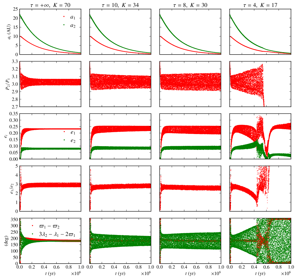
Figure 2: Semi-major axes, period ratio, eccentricities, eccentricity ratio, and angles evolution for simulations of HD~60532b, c with different dissipation timescale ratios $\tau=T_{e,1}/T_{e,2}=T_{m,1}/T_{m,2}$. The ratio $K=T_{m,i}/T_{e,i}$ is set according to Eq. (60) to reproduce the observed equilibrium eccentricities. We used $\tau=+\infty$, 10, 8, 4 with K = 70, 34, 30, 17 respectively for the four shown simulations (four columns). The amplitude of libration decreases for the first two simulations ($\tau=+\infty$, 10) and increases for the last two ($\tau=8$, 4). The value given by our analytical criterion for the transition between decreasing and increasing amplitude is $\tau\sim 9$.

The star HD~60532 hosts two planets (see Desort et al., 2008) that exhibit a 3:1 period ratio. Laskar & Correia (2009) performed a dynamical study of the system and confirmed the 3:1 MMR between the planets with a large amplitude of libration ($\sim 40^{\circ}$). We reproduced the orbital elements of the planets (taken from Laskar & Correia, 2009) in Table 1. For this system, the forced eccentricity ratio (ratio of eccentricity at the center of the resonance) is

$$\left(\frac{e_{1}}{e_{2}}\right)_{ell}\approx 3.$$ (61)

Since the system is observed with a large amplitude of libration, the stability constraint gives (Eq. (51))

$$\tau\gtrsim\left(\frac{e_{1}}{e_{2}}\right)_{ell}^{2}\approx 9.$$ (62)

Note that this value is much larger than one, thus the condition of convergent migration is fulfilled (see Eq. (54)). This value of $\tau$ corresponds to a surface density profile exponent of (see Eq. (48))

$$\beta_{\Sigma}\lesssim-1.3.$$ (63)

Let us recall that for the MMSN model $\beta_{\Sigma}=3/2$. The negative value we obtain corresponds to an inverted density profile. This inverted density profile is very untypical of type I migration. This result is thus an evidence that the planets did not undergo a classical type I migration. This is not surprising since giant planets are expected to open a gap and undergo type II migration. Our results also constrain a type II migration scenario. Indeed, independently of the migration prescriptions, for the resonance to be stable the damping of the outer eccentricity must be much more efficient than the inner eccentricity damping ($T_{e,1}/T_{e,2}\gtrsim 9$). One would need prescriptions for type II migration to relate this result with some disk and/or planets properties.

From the observed orbital elements we obtain (see Eqs. (43), (4), and (59))

$$\delta = 6.5\times 10^{-3},$$ (64)

$$C_{1} = 0.44,$$ (65)

$$C_{2} = 7.9.$$ (66)

Using $\tau\gtrsim 9$, the current eccentricities should be reproduced with (see Eq. (60))

$$K\gtrsim 30,$$ (67)

which corresponds to an aspect ratio of (see Eq. (49))

$$\frac{H}{a}\lesssim 0.18.$$ (68)

We performed numerical simulations with different values of $\tau$. For each simulation, the value of $K$ is computed using Eq. (60), in order to reproduce the equilibrium eccentricities. We fixed $T_{m,2}=5\times 10^{5}$ yr for all simulations, and integrated the system for $10^{6}$ yr. We thus have $T_{m,1}=5\times 10^{5}\tau$ yr, $T_{e,2}=5\times 10^{5}/K$ yr, $T_{e,1}=5\times 10^{5}\tau/K$ yr. The semi-major axes are initially 10 and 22 AU, such that the system is initially outside of the 3:1 resonance with a period ratio of about 3.3. Both eccentricities are initially set to 0.001 with anti-aligned periastrons and coplanar orbits. The planets are initially at periastrons (zero anomalies). The evolution of the semi-major axes, the period ratio, the eccentricities, the eccentricity ratio, and the angles are shown in Fig. 2. These simulations confirm our analytical results: for $\tau<9$, the amplitude of libration decreases, and for $\tau>9$ the amplitude increases (see Fig. 2).

5.2 GJ 876b, c: 2:1 MMR, small amplitude of libration

Table 2: Orbital parameters of GJ~876b,c used in this study (taken from Correia et al., 2010). The stellar mass is $0.334M_{\odot}$.

Parameter	[unit]	c	b
$m$	[$M_{J}$]	$0.86$	$2.64$
$P$	[day]	$30.259$	$61.065$
$a$	[AU]	$0.132$	$0.211$
$e$		$0.265$	$0.031$

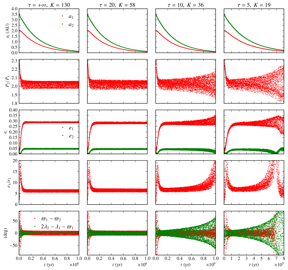
Figure 3: Same as Fig. 2 but for GJ~876b, c. We used $\tau=+\infty$, 20, 10, 5 with K = 130, 58, 36, 19 respectively for the four shown simulations (four columns). Note that the last simulation ($\tau=5$, $K=19$) ended before $10^{6}$ yr (around $8\times 10^{5}$ yr) because of orbital instability when the system escaped from resonance. The amplitude of libration decreases for the first two simulations ($\tau=+\infty$, 20) and increases for the last two ($\tau=10$, 5). The value given by our analytical criterion for the transition between decreasing and increasing amplitude is $\tau\sim 42$.

GJ~876 is a M-dwarf hosting four planets (Delfosse et al., 1998; Marcy et al., 1998, 2001; Rivera et al., 2010). The planet b and c, in which we are interested here, are Jupiter-mass planets embedded in a 2:1 MMR, while d and e are much less massive. A small amplitude of libration is observed ($\sim 5\degr$, see Correia et al., 2010) for the 2:1 resonance between GJ~876b, c. The forced eccentricity ratio is

$$\left(\frac{e_{1}}{e_{2}}\right)_{ell}\approx 6.5.$$ (69)

Since the system is observed with a small amplitude of libration, the stability constraint gives (Eq. (50))

$$\tau\gg\left(\frac{e_{1}}{e_{2}}\right)_{ell}^{2}\approx 42.$$ (70)

As for HD~60532b, c, the condition of convergent migration is fulfilled (see Eq. (54)). The surface density profile exponent is (see Eq. (48))

$$\beta_{\Sigma}\ll-5.2.$$ (71)

We obtain again a negative value that correspond to an inverted profile. We have (see Eqs. (43), (4), and (59))

$$\delta = 6.4\times 10^{-3},$$ (72)

$$C_{1} = 0.81,$$ (73)

$$C_{2} = 22.$$ (74)

Using these values and $\tau\gg 42$, we obtain (see Eq. (60))

$$K\gg 80,$$ (75)

which corresponds to an aspect ratio of (see Eq. (49))

$$\frac{H}{a}\ll 0.11.$$ (76)

As for HD~60532b, c we performed numerical simulations with different values of $\tau$ (and adjusted values of $K$ given by Eq. (60)). The semi-major axes are initially 2 and 3.5 AU (period ratio of about 2.3), the eccentricities are 0.001 with anti-aligned periastrons and coplanar orbits. The planets are initially at periastrons (zero anomalies). The evolution of the semi-major axes, the period ratio, the eccentricities, the eccentricity ratio, and the angles are shown in Fig. 3. The transition between decreasing and increasing amplitude of libration happens around $\tau\approx 20$ (see Fig. 3), while our analytical criterion gives a value of 42. Taking this refined value for $\tau$, the condition for reproducing the observed system with type I migration reads

$$\beta_{\Sigma} \ll -3.5,$$ (77)

$$K \gg 58,$$ (78)

$$\frac{H}{a} \ll 0.13.$$ (79)

The density profile still needs to be inverted ($\beta_{\Sigma}<0$) and the overall conclusions are the same.

Note that Lee & Peale (2002) studied capture scenarios for this system using a slightly different model for the migration and damping and did not observe any evolution of the libration amplitude in their simulations. The authors used constant semi-major axis ($T_{a,i}$) and eccentricity ($T_{e,i}$) damping timescales for each planet. In our study we followed the prescriptions of Papaloizou & Larwood (2000) (see also Goldreich & Schlichting, 2014) and considered constant angular momentum ($T_{m,i}$) and eccentricity ($T_{e,i}$) damping timescales. We replaced these prescriptions with Lee & Peale (2002) prescriptions for the disk-planet interactions in our analytical model (following the same scheme as described in Sect. 3.2). We found that the amplitude of libration does not evolve in this case (in agreement with Lee & Peale 2002 simulations). This difference between both prescriptions has important consequences since in the case of Lee & Peale (2002) prescriptions two initially resonant planets will stay locked in resonance forever while with the prescriptions we used the amplitude of libration can increase and the system can escape from resonance. The main difference between both prescriptions comes from the fact that with Lee & Peale (2002) prescriptions, the eccentricity damping does not affect the semi-major axes, while in our model the eccentricity damping terms contribute to the semi-major axes evolution (see Eq. (20)). Disk-planet interaction models suggest that the semi-major axes evolution are indeed influenced by the eccentricity damping effect of the disk (see Goldreich & Schlichting, 2014). We thus follow these prescriptions in our study.

5.3 HD 45364b, c: 3:2 MMR, large amplitude of libration

Table 3: Orbital parameters of HD45364b,c used in this study (taken from Correia et al., 2009). The stellar mass is $0.82M_{\odot}$.

Parameter	[unit]	c	b
$m$	[$M_{J}$]	$0.1872$	$0.6579$
$P$	[day]	$226.93$	$342.85$
$a$	[AU]	$0.6813$	$0.8972$
$e$		$0.1684$	$0.0974$

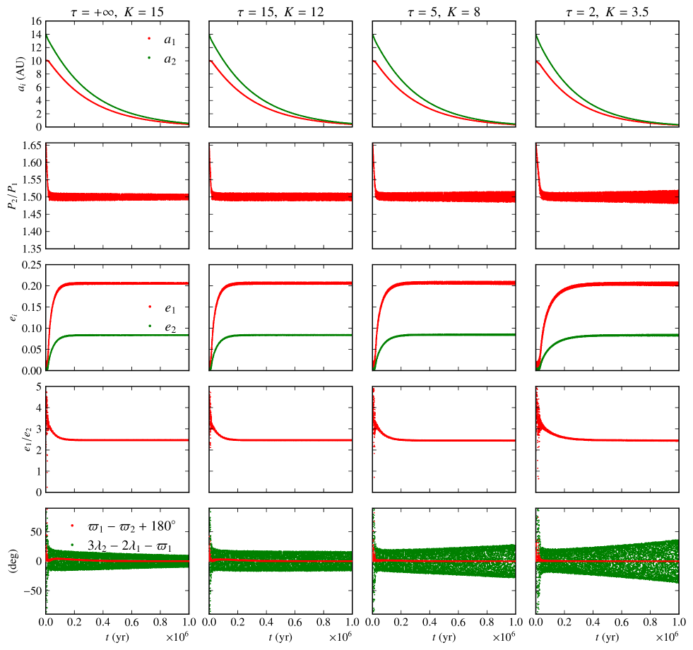
Figure 4: Same as Fig. 2 but for HD~45364b, c. We used $\tau=+\infty$, 15, 5, 2 with K = 15, 12, 8, 3.5 respectively for the four shown simulations (four columns). The amplitude of libration decreases for the first two simulations ($\tau=+\infty$, 15) and increases for the last two ($\tau=5$, 2). The value given by our analytical criterion for the transition between decreasing and increasing amplitude is $\tau\sim 6.3$.

The star HD~45364 hosts two planets (Correia et al., 2009) embedded in a 3:2 MMR. The forced eccentricity ratio is

$$\left(\frac{e_{1}}{e_{2}}\right)_{ell}\approx 2.5.$$ (80)

A large amplitude of libration is observed ($\sim 70\degr$, see Correia et al., 2009), thus, the stability constraint gives (Eq. (51))

$$\tau\gtrsim\left(\frac{e_{1}}{e_{2}}\right)_{ell}^{2}\approx 6.3.$$ (81)

The condition of convergent migration is fulfilled (see Eq. (54)). The surface density profile exponent is (see Eq. (48))

$$\beta_{\Sigma}\lesssim-1.6.$$ (82)

We obtain again a negative value that corresponds to an inverted profile. We have (see Eqs. (43), (4), and (59))

$$\delta = 6.0\times 10^{-3},$$ (83)

$$C_{1} = 0.93,$$ (84)

$$C_{2} = 2.3.$$ (85)

Using these values and $\tau\gtrsim 6.3$, we obtain (see Eq. (60))

$$K\gtrsim 9.4,$$ (86)

which corresponds to an aspect ratio of (see Eq. (49))

$$\frac{H}{a}\lesssim 0.33.$$ (87)

We performed numerical simulations with different values of $\tau$ and $K$ (given by Eq. (60)). The semi-major axes are initially 10 and 14 AU (period ratio of about 1.65), the eccentricities are 0.001 with anti-aligned periastrons and coplanar orbits. The planets are initially at periastrons (zero anomalies). The evolution of the semi-major axes, the period ratio, the eccentricities, the eccentricity ratio, and the angles are shown in Fig. 4. According to our simulations, the amplitude of libration increases for $\tau\lesssim 10$ (transition between 5-15, see Fig. 4) which is comparable with our analytical result ($\tau\lesssim 6.3$).

It may seem surprising that the amplitude of libration does not increase much more rapidly for $\tau=2$ than for $\tau=5$ (see Fig. 4). Indeed, our study shows that the smaller $\tau$ is, the more unstable the resonant configuration is (Eq. (35)). However, the evolution of the amplitude of libration does not only depend on the ratio $\tau=T_{e,1}/T_{e,2}$ but also on the absolute values of these damping timescales (see Eq. (35)). In our simulations, we fixed the migration timescale for the outer planet ($T_{m,2}$) and varied the three other timescales: $T_{m,1}=\tau T_{m,2}$, $T_{e,2}=T_{m,2}/K$, $T_{e,1}=\tau T_{m,2}/K$. The damping timescales are thus much longer for the simulation with $\tau=2$ ($K=3.5$) than for $\tau=5$ ($K=8$), in order to reproduce the same equilibrium eccentricities. This tends to slow down the increasing of the amplitude of libration and compensates the acceleration provided by decreasing $\tau$.

6 Conclusion

We obtained a simple analytical criterion for the stability of the resonant configuration between two planets during their migration in a protoplanetary disk. We used the simplified integrable model of mean-motion resonances that we developed in Delisle et al. (2014), and modeled the dissipative effect of the disk on the planets by four distinct timescales: $T_{m,1}$, $T_{m,2}$ (migration of both planets), and $T_{e,1}$, $T_{e,2}$ (damping of both eccentricities). As shown by Lee & Peale (2002), migrating planets that are captured in resonance have their eccentricities excited by the migration forces of the disk. The eccentricities reach equilibrium values between the migration and damping forces. However, this equilibrium can be unstable, in which case the amplitude of libration in the resonance increases until the system crosses the separatrix and escapes from resonance (Goldreich & Schlichting, 2014). We showed here that the equilibrium is stable on the condition that $T_{e,1}/T_{e,2}>(e_{1}/e_{2})^{2}_{ell}$ (ratio of equilibrium eccentricities). For observed resonant systems, it is probable that the equilibrium was stable during the migration phase. Otherwise, the planets would have escaped from resonance. This result allows to put constraints on the damping forces undergone by the planets. For instance, using prescriptions for type I migration, we show that a locally inverted profile is needed for resonant systems for which the inner planet angular momentum deficit (AMD) is larger than the outer planet AMD. We applied our analytical criterion to HD~60532b, c (3:1 MMR), GJ~876b, c (2:1 MMR), and HD~45364b, c (3:2 MMR). We showed for all studied systems that if the planets had undergone type I migration, an inverted density profile would be required for the resonant configuration to be stable. All these planets are Jupiter-mass planets and are thus believed to open a gap in the disk and undergo type II migration. Our results confirm that classical type I migration cannot reproduce the observed systems.

Our model is very general and is not restricted to type I migration. Considering a scenario of type II migration which is much more realistic for the studied systems, our model still gives constraints on the migration process and especially on the eccentricity damping undergone by each planet. However, we could not find a simple analytical prescription for type II migration in the literature and thus could not derive constraints on the disk properties in this case. Having analytical prescriptions for type II migration would allow a more detailed analysis of these systems.

It would also be very interesting in the future to study small planets in resonance (with precise enough determination of orbital parameters to be sure of the resonant motion). Indeed, for small planets, a type I migration scenario is more realistic. In this case, a local inversion of the density profile (as needed for the three systems of this study) would be more surprising.

Appendix A Renormalization of coordinates

The renormalized variables are constructed by dividing all actions by the following constant of motion (see Delisle et al. 2012, 2014)

$$\Gamma=\frac{k_{2}}{k_{1}}\hat{\Lambda}_{1}+\hat{\Lambda}_{2},$$ (88)

where $\hat{\Lambda}_{i}=\beta_{i}\sqrt{\mu_{i}a_{i}}$ is the circular angular momentum of the planet $i$. Noting with a hat the initial actions, the renormalized ones are defined by

$$\Lambda_{i} = \frac{\hat{\Lambda}_{i}}{\Gamma},$$ (89)

$$G_{i} = \frac{\hat{G}_{i}}{\Gamma},$$ (90)

$$I_{i} = \frac{\hat{I}_{i}}{\Gamma},$$ (91)

$$\mathcal{D} = \frac{\hat{\mathcal{D}}}{\Gamma},$$ (92)

$$\delta = \frac{\hat{\delta}}{\Gamma}.$$ (93)

Expressions (2) and (2) are straightforwardly derived from these definitions.

Note that the Hamiltonian and the time also have to be renormalized (see Delisle et al. 2012, 2014) in order to preserve Hamiltonian properties. However, in this study, we consider dissipative forces that act on the system on very long timescales. As long as the conservative timescale remains short compared to the dissipation timescale, the long term evolution of the system is well described by the mean effect of the dissipation over the conservative timescale. Therefore, the rescaling of this conservative timescale will not influence the long term evolution of the system.

Appendix B Reducing to an integrable problem

In the general case, the motion of two planets in a $k_{2}$:$k_{1}$ resonance is described by two degrees of freedom, i.e. both resonant angles

$$\sigma_{1} = \frac{k_{2}}{q}\lambda_{2}-\frac{k_{1}}{q}\lambda_{1}-\varpi_{1},$$ (94)

$$\sigma_{2} = \frac{k_{2}}{q}\lambda_{2}-\frac{k_{1}}{q}\lambda_{1}-\varpi_{2},$$ (95)

and both actions $I_{1}$, $I_{2}$. Let us note $x_{i}$ the complex cartesian coordinates associated to these action-angle coordinates

$$x_{i}=\sqrt{I_{i}}\mathbf{e}^{\mathbf{i}\sigma_{i}}.$$ (96)

The simplifying assumption introduced in Delisle et al. (2014) allows to reduce this generally non-integrable problem to a single degree of freedom one (thus integrable). The only remaining resonant angle is $\theta$ and the associated action is $\mathcal{D}$. Noting $u$ the related complex cartesian coordinate

$$u=\sqrt{\mathcal{D}}\mathbf{e}^{\mathbf{i}\theta},$$ (97)

the simplifying assumption reads

$$0 = \cos\phi\mathbf{e}^{-\mathbf{i}\sigma_{2,ell}}x_{2}-\sin\phi\mathbf{e}^{-\mathbf{i}\sigma_{1,ell}}x_{1},$$ (98)

$$u = \cos\phi\mathbf{e}^{-\mathbf{i}\sigma_{1,ell}}x_{1}+\sin\phi\mathbf{e}^{-\mathbf{i}\sigma_{2,ell}}x_{2},$$ (99)

where $\phi$, $\sigma_{1,ell}$, $\sigma_{2,ell}$ are constant angles defined such that the libration center is directed toward $u$ (see Delisle et al. 2014). Equation (99) shows how the simplified one degree of freedom model mixes both initial degrees of freedom, and especially, how the resonant angle $\theta$ mixes both initial resonant angles $\sigma_{1}$, $\sigma_{2}$. Equation (10) directly results from Eq. (98).

Appendix C Evolution of the parameter $\delta$ under dissipation

In this section we show how to compute the evolution of the parameter $\delta$ (Eq. (3.1)) under a dissipation affecting the semi-major axes and eccentricities of the planets. The evolution of the renormalized circular angular momenta only depends on $(\alpha/\dot{\alpha})_{d}$. These renormalized quantities are constructed such that (see Appendix A and Delisle et al. 2014)

$$\frac{\Lambda_{1}}{\Lambda_{2}}=\frac{\beta_{1}\sqrt{\mu_{1}}}{\beta_{2}\sqrt{\mu_{2}}}\sqrt{\alpha}\approx\frac{m_{1}}{m_{2}}\sqrt{\alpha},$$ (100)

and

$$\frac{k_{2}}{k_{1}}\Lambda_{1}+\Lambda_{2}=1.$$ (101)

We deduce

$$\dot{\Lambda}_{1}|_{d} = \frac{\Lambda_{1}\Lambda_{2}}{2}\left.\frac{\dot{\alpha}}{\alpha}\right|_{d},$$ (102)

$$\dot{\Lambda}_{2}|_{d} = -\frac{k_{2}}{k_{1}}\frac{\Lambda_{1}\Lambda_{2}}{2}\left.\frac{\dot{\alpha}}{\alpha}\right|_{d}.$$ (103)

The evolution of $\epsilon$ is then straightforward (see Eq. (2))

$$\dot{\epsilon}|_{d}=\dot{\Lambda}_{1}|_{d}+\dot{\Lambda}_{2}|_{d}=-\frac{q}{k_{1}}\frac{\Lambda_{1}\Lambda_{2}}{2}\left.\frac{\dot{\alpha}}{\alpha}\right|_{d}.$$ (104)

The evolution of the renormalized deficit of angular momentum $I_{i}$ is given by

$$\left.\frac{\dot{I}_{i}}{I_{i}}\right|_{d}=2\left.\frac{\dot{\xi}_{i}}{\xi_{i}}\right|_{d}+\left.\frac{\dot{\Lambda}_{i}}{\Lambda_{i}}\right|_{d},$$ (105)

$$\left.\frac{\dot{I}_{1}}{I_{1}}\right|_{d}=2\left.\frac{\dot{\xi}_{1}}{\xi_{1}}\right|_{d}+\frac{\Lambda_{2}}{2}\left.\frac{\dot{\alpha}}{\alpha}\right|_{d},$$ (106)

$$\left.\frac{\dot{I}_{2}}{I_{2}}\right|_{d}=2\left.\frac{\dot{\xi}_{2}}{\xi_{2}}\right|_{d}-\frac{k_{2}}{k_{1}}\frac{\Lambda_{1}}{2}\left.\frac{\dot{\alpha}}{\alpha}\right|_{d}=2\left.\frac{\dot{\xi}_{2}}{\xi_{2}}\right|_{d}+\frac{\Lambda_{2}-1}{2}\left.\frac{\dot{\alpha}}{\alpha}\right|_{d}.$$ (107)

We thus deduce

$$\left.\frac{\dot{\mathcal{D}}}{\mathcal{D}}\right|_{d} = \cos^{2}\phi\left.\frac{\dot{I}_{1}}{I_{1}}\right|_{d}+\sin^{2}\phi\left.\frac{\dot{I}_{2}}{I_{2}}\right|_{d}$$

$$= 2\left(\cos^{2}\phi\left.\frac{\dot{\xi}_{1}}{\xi_{1}}\right|_{d}+\sin^{2}\phi\left.\frac{\dot{\xi}_{2}}{\xi_{2}}\right|_{d}\right)$$

$$+\frac{\Lambda_{2}-\sin^{2}\phi}{2}\left.\frac{\dot{\alpha}}{\alpha}\right|_{d}.$$

Finally, we have

$$\dot{\delta}|_{d} = \dot{\mathcal{D}}|_{d}-\dot{\epsilon}|_{d}$$

$$= 2\left(\cos^{2}\phi\left.\frac{\dot{\xi}_{1}}{\xi_{1}}\right|_{d}+\sin^{2}\phi\left.\frac{\dot{\xi}_{2}}{\xi_{2}}\right|_{d}\right)\mathcal{D}$$

$$+\frac{\Lambda_{2}-\sin^{2}\phi}{2}\left.\frac{\dot{\alpha}}{\alpha}\right|_{d}\mathcal{D}$$

$$+\frac{q}{k_{1}}\frac{\Lambda_{1}\Lambda_{2}}{2}\left.\frac{\dot{\alpha}}{\alpha}\right|_{d}.$$