HAT-P-55b: A Hot Jupiter Transiting a Sun-Like Star

Abstract

We report the discovery of a new transiting extrasolar planet, HAT-P-55b. The planet orbits a V = $13.207\pm 0.039$ sun-like star with a mass of $1.013\pm 0.037$ $M_{\sun}$, a radius of $1.011\pm 0.036$ $R_{\sun}$ and a metallicity of $-0.03$ $\pm$ $0.08$. The planet itself is a typical hot Jupiter with a period of $3.5852467\pm 0.0000064$ days, a mass of $0.582\pm 0.056$ $M_{\rm J}$ and a radius of $1.182\pm 0.055$ $R_{\rm J}$. This discovery adds to the increasing sample of transiting planets with measured bulk densities, which is needed to put constraints on models of planetary structure and formation theories.

1. Introduction

Today we know of almost 1800 validated exoplanets and more than 4000 exoplanet candidates. Among these, the transiting exoplanets (TEPs) are essential in our exploration and understanding of the physical properties of exoplanets. While radial velocity observations alone only allow us to estimate the minimum mass of a planet, we can combine them with transit observations for a more comprehensive study of the physical properties of the planet. When a planet transits, we can determine the inclination of the orbit and the radius of the planet, allowing us to break the mass degeneracy and, along with the mass, determine the mean density of the planet. The mean density of a planet offers us insight into its interior composition, and although there is an inherent degeneracy arising from the fact that planets of different compositions can have identical masses and radii, this information allows us to map the diversity and distribution of exoplanets and even put constraints on models of planetary structure and formation theories.

The occurrence rate of hot Jupiters in the Solar neighbourhood is around 1% (Udry & Santos 2007; Wright et al. 2012). With a transit probability of about $\sim$10$\%$, roughly one thousand stars need to be monitored in photometry to find just a single hot Jupiter. Therefore, the majority of the known transiting hot Jupiters have been discovered by photometric wide field surveys targeting tens of thousands of stars per night.

In this paper we present the discovery of HAT-P-55b by the Hungarian-made Automated Telescope Network (HATNet; see Bakos et al. 2004), a network of six small fully automated wide field telescopes of which four are located at the Fred Lawrence Whipple Observatory in Arizona, and two are located at the Mauna Kea Observatory in Hawaii. Since HATNet saw first light in 2003, it has searched for TEPs around bright stars (V $\lesssim$ 13) covering about 37% of the Northern sky, and discovered approximately 25% of the known transiting hot Jupiters.

The layout of the paper is as follows. In Section 2 we present the different photometric and spectroscopic observations that lead to the detection and characterisation of HAT-P-55b. In Section 3 we derive the stellar and planetary parameters. Finally, we discuss the characteristics of HAT-P-55b in Section 4.

2. Observations

The general observational procedure used by HATNet to discover TEPs has been described in detail in previous papers (e.g. Bakos et al. 2010; Latham et al. 2009). In this section we present the specific details for the discovery and follow-up observations of HAT-P-55b.

2.1. Photometry

2.1.1 Photometric detection

HAT-P-55b was initially identified as a candidate transiting exoplanet based on photometric observations made by the HATNet survey (Bakos et al., 2004) in 2011. The observations of HAT-P-55 were made on nights between February and August with the HAT-5 telescope at the Fred Lawrence Whipple Observatory (FLWO) in Arizona, and on nights between May and August with the HAT-8 telescope at Mauna Kea Observatory in Hawaii. Both telescopes used a Sloan $r$ band filter. HAT-5 provided a total of 10574 images with a median cadence of 218s, and HAT-8 provided a total of 6428 images with a median cadence of 216s.

The results were processed and reduced to trend-filtered light curves using the External Parameter Decorrelation method (EPD; see Bakos et al. 2010) and the Trend Filtering Algorithm (TFA; see Kovács et al. 2005). The light curves were searched for periodic transit signals using the Box Least-Squares method (BLS; see Kovács et al. 2002). The individual photometric measurements for HAT-P-55 are listed in Table 2.1.2, and the folded light curves together with the best-fit transit light curve model are presented in Figure 1.

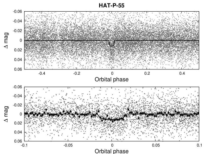
Figure 1.— HATNet light curve of HAT-P-55 phase folded with the transit period. The top panel shows the unbinned light curve, while the bottom panel shows the region zoomed-in on the transit, with dark filled circles for the light curve binned in phase with a binsize of 0.002. The solid line represents the best-fit light curve model.

2.1.2 Photometric follow-up

We performed photometric follow-up observations of HAT-P-55 using the KeplerCam CCD camera on the 1.2 m telescope at the FLWO, observing a transit ingress on the night of 23 May 2013, and a full transit on the night of 7 April 2014. Both transits were observed using a Sloan $i$-band filter. For the first event we obtained 230 images with a median cadence of 64s, and for the second event we obtained 258 images with a median cadence of 67s.

The results were reduced to light curves following the procedure of Bakos et al. (2010), and EPD and TFA were performed to remove trends simultaneously with the light curve modelling. The individual photometric follow-up measurements for HAT-P-55 are listed in Table 2.1.2, and the folded light curves together with our best-fit transit light curve model are presented in Figure 2.

Subtracting the transit signal from the HATNet light curve, we used the BLS method to search for additional transit signals and found none. A Discrete Fourier Transform also revealed no other periodic signals in the data.

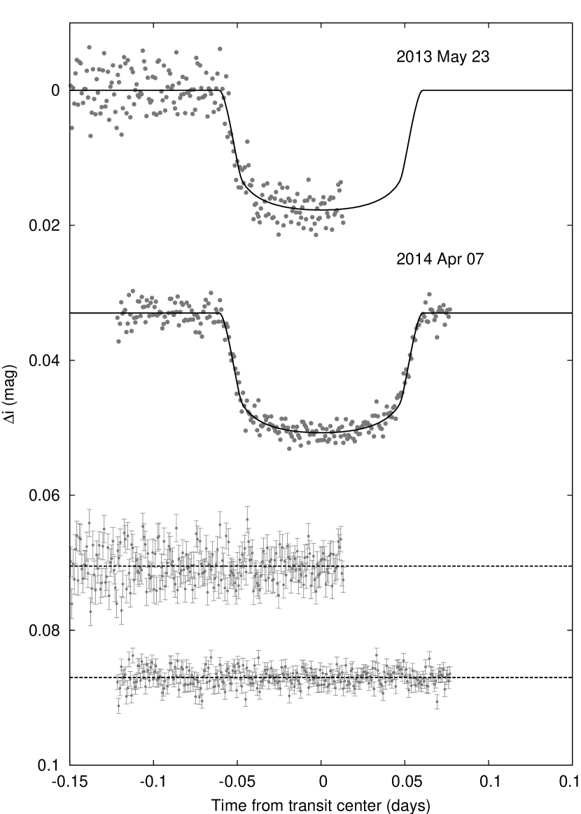
Figure 2.— Unbinned transit light curves for HAT-P-55, acquired with KeplerCam at the FLWO 1.2 m telescope. The light curves have been EPD- and TFA-processed, as described in Bakos et al. (2010). The solid lines represents the best fit from the global modeling described in Section 3. Residuals from the fit are displayed below at the bottom of the figure. The error bars represent the photon and background shot noise, plus the readout noise.

Table 1 Differential photometry of HAT-P-55.

BJD	Mag	$\sigma_{\rm Mag}$	Mag(orig)	Filter	Instrument
(2,400,000$+$)
$55667.80829$	$-0.01089$	$0.02455$	$\cdots$	$r$	HATNet
$55649.88231$	$0.00947$	$0.01537$	$\cdots$	$r$	HATNet
$55778.95165$	$0.02246$	$0.01538$	$\cdots$	$r$	HATNet
$55692.90580$	$-0.00422$	$0.01713$	$\cdots$	$r$	HATNet
$55735.92912$	$0.00602$	$0.02207$	$\cdots$	$r$	HATNet
$55771.78174$	$-0.01054$	$0.01241$	$\cdots$	$r$	HATNet
$55710.83270$	$-0.01741$	$0.01609$	$\cdots$	$r$	HATNet
$55674.98046$	$0.01418$	$0.01771$	$\cdots$	$r$	HATNet
$55728.75933$	$0.04136$	$0.03816$	$\cdots$	$r$	HATNet
$55710.83315$	$0.00822$	$0.01348$	$\cdots$	$r$	HATNet

Note. — This table is available in a machine-readable form in the online journal. A portion is shown here for guidance regarding its form and content.

Table 2 Relative radial velocities, and bisector span measurements of HAT-P-55.

2.2. Spectroscopy

We performed spectroscopic follow-up observations of HAT-P-55 to rule out false positives and to determine the RV variations and stellar parameters. Initial reconnaissance observations were carried out with the Tillinghast Reflector Echelle Spectrograph (TRES; Fűrész 2008) at the FLWO. We obtained 2 spectra near opposite quadratures on the nights of 4 and 31 October 2012. Using the Stellar Parameters Classification method (SPC; see Buchhave et al. 2012), we determined the initial RV measurements and stellar parameters. We found a mean absolute RV of $-9.42$ km s^-1 with an rms of 48 m s^-1, which is consistent with no detectable RV variation. The stellar parameters, including the effective temperature $T_{\rm eff\star}$= 5800 $\pm$ 50 K, surface gravity $\log{g_{\star}}$= 4.5 $\pm$ 0.1 (log cgs) and projected rotational velocity $v\sin{i}$= 5.0 $\pm$ 0.4 km s^-1, correspond to those of a G2 dwarf.

High-resolution spectroscopic observations were then carried out with the SOPHIE spectrograph mounted on the 1.93 m telescope at Observatoire de Haute-Provence (OHP) (Perruchot et al., 2011; Bouchy et al., 2013), and with the FIES spectrograph mounted on the 2.6 m Nordic Optical Telescope (Djupvik & Andersen, 2010). We obtained 6 SOPHIE spectra on nights between 3 June and 12 June 2013, and 10 FIES spectra on nights between 15 May and 26 August 2013.

We reduced and extracted the spectra and derived radial velocities and spectral line bisector span (BS) measurements following the method of Boisse et al. (2013) for the SOPHIE data and the method of Buchhave et al. (2010) for the FIES data. The final RV data and their errors are listed for both instruments in Table 2.1.2, and

the folded RV data together with our best-fit orbit and corresponding residuals and bisectors are presented in Figure 3. To avoid underestimating the BS uncertainties we base them directly on the RV uncertainties, setting them equal to twice the RV uncertainties. At a first glance there do seem to be a slight hint of variation of the BSs in phase with the RVs suggesting there might be a blend. This is not the case, however, as will we show in our detailed blend analysis in Section 3.

We applied the SPC method to the FIES spectra to determine the final spectroscopic parameters of HAT-P-55. The values were calculated using a weighted mean, taking into account the cross correlation function (CCF) peak height. The results are shown in Table 3.

Figure 3.— Top panel: RV measurements from NOT 2.6 m/FIES (filled circles) and OHP 1.93 m/SOPHIE (open triangles) for HAT-P-55 shown as a function of orbital phase, along with our best-fit circular model (solid line; see Table 4). Zero phase corresponds to the time of mid-transit. The center-of-mass velocity has been subtracted. Second panel: RV residuals from our best-fit circular model. The error bars include a “jitter” component ($0.0\pm 3.1$ $\rm m\,s^{-1}$, and $26\pm 13$ $\rm m\,s^{-1}$ for FIES and SOPHIE respectively) added in quadrature to the formal errors (see Section 2.2). The symbols are as in the upper panel. Third panel: Bisector spans (BS), adjusted to have a median of 0. Bottom panel: RV residuals from our best-fit circular model vs. BS. There is no sign of correlation. Note the different vertical scales of the panels.

3. Analysis

In order to rule out the possibility that HAT-P-55 is a blended stellar eclipsing binary system, and not a transiting planet system, we carried out a blend analysis following Hartman et al. (2012). We find that a single star with a transiting planet fits the light curves and catalog photometry better than models involving a stellar eclipsing binary blended with light from a third star. While it is possible to marginally fit the photometry using a G star eclipsed by a late M dwarf that is blended with another bright G star, simulated spectra for this scenario are obviously composite and show large (multiple $\rm km\,s^{-1}$) bisector span and RV variations that are inconsistent with the observations. Based on this analysis we conclude that HAT-P-55 is not a blended stellar eclipsing binary system, and is instead best explained as a transiting planet system. We also consider the possibility that HAT-P-55 is a planetary system with a low-mass stellar companion that has not been spatially resolved. The constraint on this scenario comes from the catalog photometric measurements, based on which we can exclude a physical companion star with a mass greater than $0.7$ $M_{\sun}$. Any companion would dilute both the photometric transit and radial velocity orbit. The maximum dilution allowed by the photometry would increase the planetary radius by $\sim$15%.

We analyzed the system following the procedure of Bakos et al. (2010) with modifications described in Hartman et al. (2012). In short, we (1) determined the stellar atmospheric parameters of the host star HAT-P-55 by applying the SPC method to the FIES spectra; (2) used a Differential Evolution Markov-Chain Monte Carlo procedure to simultaneously model the RVs and the light curves, keeping the limb darkening coefficients fixed to those of the Claret (2004) tabulations; (3) used the spectroscopically inferred effective temperatures and metallicities of the star, the stellar densities determined from the light curve modeling, and the Yonsei-Yale theoretical stellar evolution models (Yi et al., 2001) to determine the stellar mass, radius and age, as well as the planetary parameters (e.g. mass and radius) which depend on the stellar values (Figure 4).

Figure 4.— Comparison between the measured values of $T_{\rm eff\star}$ and $\rho_{\star}$ (from SPC applied to the FIES spectra, and from our modeling of the light curves and RV data, respectively), and the Y² model isochrones from Yi et al. (2001). The best-fit values, and approximate 1$\sigma$ and 2$\sigma$ confidence ellipsoids are shown. The Y² isochrones are shown for ages of 0.2 Gyr, and 1.0 to 14.0 Gyr in 1 Gyr increments.

Table 3 Stellar Parameters for HAT-P-55

Parameter	Value	Source
Identifying Information
R.A. (h:m:s)	$17^{\mathrm{h}}37^{\mathrm{m}}05.52{\mathrm{s}}$	2MASS
Dec. (d:m:s)	$+25{\arcdeg}43{\arcmin}52.3{\arcsec}$	2MASS
GSC ID	GSC 2080-00517	GSC
2MASS ID	2MASS 17370562+2543522	2MASS
HTR ID	HTR 287-004	HATNet
Spectroscopic properties
$T_{\rm eff\star}$ (K)	$5808\pm 50$	SPC
$\rm[Fe/H]$	$-0.030\pm 0.080$	SPC
$v\sin{i}$ ($\rm km\,s^{-1}$)	$1.80\pm 0.50$	SPC
$\gamma_{\rm RV}$ ($\rm km\,s^{-1}$)	$-9.42\pm 0.05$	TRES
Photometric properties
$B$ (mag)	$13.871\pm 0.039$	APASS
$V$ (mag)	$13.207\pm 0.039$	APASS
$I$ (mag)	$12.67\pm 0.14$	TASS
$g$ (mag)	$13.50\pm 0.04$	APASS
$r$ (mag)	$13.06\pm 0.02$	APASS
$i$ (mag)	$12.88\pm 0.04$	APASS
$J$ (mag)	$12.020\pm 0.022$	2MASS
$H$ (mag)	$11.714\pm 0.026$	2MASS
$K_{s}$ (mag)	$11.627\pm 0.025$	2MASS
Derived properties
$M_{\star}$ ($M_{\sun}$)	$1.013\pm 0.037$	Isochrones+$\rho_{\star}$+SPC
$R_{\star}$ ($R_{\sun}$)	$1.011\pm 0.036$	Isochrones+$\rho_{\star}$+SPC
$\log{g_{\star}}$ (cgs)	$4.434\pm 0.032$	Isochrones+$\rho_{\star}$+SPC
$L_{\star}$ ($L_{\sun}$)	$1.042\pm 0.089$	Isochrones+$\rho_{\star}$+SPC
$M_{V}$ (mag)	$4.785\pm 0.097$	Isochrones+$\rho_{\star}$+SPC
$M_{K}$ (mag,ESO)	$3.266\pm 0.081$	Isochrones+$\rho_{\star}$+SPC
Age (Gyr)	$4.2\pm 1.7$	Isochrones+$\rho_{\star}$+SPC
$A_{V}$ (mag)	$0.020_{-0.020}^{+0.060}$	Isochrones+$\rho_{\star}$+SPC
Distance (pc)	$480\pm 19$	Isochrones+$\rho_{\star}$+SPC
$\log{R^{\prime}_{\textrm{HK}}}$	$-5.0\pm 0.1$	Boisse et al 2010

Table 4Parameters for the transiting planet HAT-P-55b.

Parameter	Value
Light curve parameters
$P$ (days)	$3.5852467\pm 0.0000064{}$
$T_{c}$ (${\rm BJD}$)	$2456730.83468\pm 0.00027{}$
$T_{14}$ (days)	$0.1223\pm 0.0013{}$
$T_{12}=T_{34}$ (days)	$0.0152\pm 0.0013{}$
$a/R_{\star}$	$9.79\pm 0.34{}$
$\zeta/R_{\star}$	$18.64\pm 0.10{}$0
$R_{p}/R_{\star}$	$0.1202\pm 0.0019{}$
$b^{2}$	$0.153_{-0.060}^{+0.062}{}$
$b\equiv a\cos i/R_{\star}$	$0.392_{-0.086}^{+0.073}{}$
$i$ (deg)	$87.70\pm 0.56{}$0
Limb-darkening coefficients
$c_{1},i$ (linear term)	$0.2619{}$
$c_{2},i$ (quadratic term)	$0.3313{}$
$c_{1},r$	$0.3466{}$
$c_{2},r$	$0.3306{}$
RV parameters
$K$ ($\rm m\,s^{-1}$)	$76.7\pm 7.1{}$00
$e$	$<0.139{}$
RV jitter NOT 2.6 m/FIES ($\rm m\,s^{-1}$)	$0.0\pm 3.1$
RV jitter OHP 1.93 m/SOPHIE ($\rm m\,s^{-1}$)	$26\pm 13$
Planetary parameters
$M_{p}$ ($M_{\rm J}$)	$0.582\pm 0.056{}$
$R_{p}$ ($R_{\rm J}$)	$1.182\pm 0.055{}$
$C(M_{p},R_{p})$	$-0.01{}$
$\rho_{p}$ ($\rm g\,cm^{-3}$)	$0.435\pm 0.077{}$
$\log g_{p}$ (cgs)	$3.012\pm 0.060{}$
$a$ (AU)	$0.04604\pm 0.00056{}$
$T_{\rm eq}$ (K)	$1313\pm 26{}$
$\Theta$	$0.0446\pm 0.0048{}$
$\langle F\rangle$ ($10^{9}$$\rm erg\,s^{-1}\,cm^{-2}$)	$6.71\pm 0.53{}$

We conducted the analysis inflating the SOPHIE and FIES RV uncertainties by adding a ”jitter” term in quadrature to the formal uncertainties. This was done to accommodate the larger than expected scattering of the RV observations around the best-fit model. Independent jitters were used for each instrument, as it is not clear whether the jitter is instrumental or astrophysical in origin. The jitter term was allowed to vary in the fit, yielding a $\chi^{2}$ per degree of freedom of unity for the RVs in the best-fit model. The median values for the jitter are $26\pm 13$ $\rm m\,s^{-1}$ for the SOPHIE observations and $0.0\pm 3.1$ $\rm m\,s^{-1}$ for the FIES observations. This suggests that either the formal uncertainties of the FIES instrument were overestimated, or that the jitter from the SOPHIE instrument is not from the star but from the instrument itself.

The analysis was done twice: fixing the eccentricity to zero, and allowing it to vary. Computing the Bayesian evidence for each model, we found that the fixed circular model is preferred by a factor of $\sim$500. Therefore the circular orbit model was adopted. The $95\%$ confidence upper limit on the eccentricity is $e<0.139{}$.

The best-fit models are presented in Figures 1, 2 and 3, and the resulting derived stellar and planetary parameters are listed in Tables 3 and 4, respectively. We find that the star HAT-P-55 has a mass of $1.013\pm 0.037{}$ $M_{\sun}$ and a radius of $1.011\pm 0.036{}$ $R_{\sun}$, and that its planet HAT-P-55b has a period of $3.5852467\pm 0.0000064$ days, a mass of $0.582\pm 0.056{}$ $M_{\rm J}$ and a radius of $1.182\pm 0.055{}$ $R_{\rm J}$.

4. Discussion

We have presented the discovery of a new transiting planet, HAT-P-55b, and provided a precise characterisation of its properties. HAT-P-55b is a moderately inflated $\sim$0.5 $M_{\rm J}$ planet, similar in mass, radius and equilibrium temperature to HAT-P-1b (Bakos et al., 2007), WASP-34 (Smalley et al., 2011), and HAT-P-25b (Quinn et al., 2012).

With a visual magnitude of V = 13.21, HAT-P-55b is among the faintest transiting planet host stars discovered by a wide field ground-based transit survey (today, a total of 11 transiting planet host stars with V $>$ 13 have been discovered by wide-field ground based transit surveys, the faintest one is HATS-6 with V = 15.2 (Hartman et al., 2014)). Of course, V $>$ 13 is only faint by the standards of surveys like HATNet and WASP; most of the hundreds of transiting planets found by space-based surveys such as OGLE, CoRoT and Kepler have host stars fainter than HAT-P-55. It is worth noticing that despite the relative faintness of HAT-P-55, the mass and radius of HAT-P-55b has been measured to better than 10% precision (relative to the precision of the stellar parameters) using modest-aperture facilities. This achievement was possible because the relatively large size of the planet to its host star provided for a strong and therefore easy to measure signal. In comparison, only about 140 of all the 1175 known TEP’s have masses and radii measured to better than 10% precision.

Acknowledgements

HATNet operations have been funded by NASA grants NNG04GN74G and NNX13AJ15G. Follow-up of HATNet targets has been partially supported through NSF grant AST-1108686. G.Á.B., Z.C. and K.P. acknowledge partial support from NASA grant NNX09AB29G. K.P. acknowledges support from NASA grant NNX13AQ62G. G.T. acknowledges partial support from NASA grant NNX14AB83G. D.W.L. acknowledges partial support from NASA’s Kepler mission under Cooperative Agreement NNX11AB99A with the Smithsonian Astrophysical Observatory. D.J. acknowledges the Danish National Research Foundation (grant number DNRF97) for partial support.

Data presented in this paper are based on observations obtained at the HAT station at the Submillimeter Array of SAO, and the HAT station at the Fred Lawrence Whipple Observatory of SAO. Data are also based on observations with the Fred Lawrence Whipple Observatory 1.5m and 1.2m telescopes of SAO. This paper presents observations made with the Nordic Optical Telescope, operated on the island of La Palma jointly by Denmark, Finland, Iceland, Norway, and Sweden, in the Spanish Observatorio del Roque de los Muchachos of the Instituto de Astrofísica de Canarias. The authors thank all the staff of Haute-Provence Observatory for their contribution to the success of the ELODIE and SOPHIE projects and their support at the 1.93-m telescope. The research leading to these results has received funding from the European Community’s Seventh Framework Programme (FP7/2007-2013) under grant agreement number RG226604 (OPTICON). The authors wish to recognize and acknowledge the very significant cultural role and reverence that the summit of Mauna Kea has always had within the indigenous Hawaiian community. We are most fortunate to have the opportunity to conduct observations from this mountain.

References

- Bakos et al. (2004) Bakos, G., Noyes, R. W., Kovács, G., et al. 2004, PASP, 116, 266
- Bakos et al. (2007) Bakos, G. Á., Noyes, R. W., Kovács, G., et al. 2007, ApJ, 656, 552
- Bakos et al. (2010) Bakos, G. Á., Torres, G., Pál, A., et al. 2010, ApJ, 710, 1724
- Boisse et al. (2013) Boisse, I., Hartman, J. D., Bakos, G. Á., et al. 2013, A&A, 558, A86
- Bouchy et al. (2013) Bouchy, F., Díaz, R. F., Hébrard, G., et al. 2013, A&A, 549, A49
- Buchhave et al. (2010) Buchhave, L. A., Bakos, G. Á., Hartman, J. D., et al. 2010, ApJ, 720, 1118
- Buchhave et al. (2012) Buchhave, L. A., Latham, D. W., Johansen, A., et al. 2012, Nature, 486, 375
- Cardelli et al. (1989) Cardelli, J. A., Clayton, G. C., & Mathis, J. S. 1989, ApJ, 345, 245
- Claret (2004) Claret, A. 2004, A&A, 428, 1001
- Djupvik & Andersen (2010) Djupvik, A. A., & Andersen, J. 2010, in Highlights of Spanish Astrophysics V, ed. J. M. Diego, L. J. Goicoechea, J. I. González-Serrano, & J. Gorgas, 211
- Fűrész (2008) Fűrész, G. 2008, PhD thesis, Univ. of Szeged, Hungary
- Hansen & Barman (2007) Hansen, B. M. S., & Barman, T. 2007, ApJ, 671, 861
- Hartman et al. (2012) Hartman, J. D., Bakos, G. Á., Béky, B., et al. 2012, AJ, 144, 139
- Hartman et al. (2014) Hartman, J. D., Bayliss, D., Brahm, R., et al. 2014, ArXiv e-prints, 1408.1758
- Kovács et al. (2005) Kovács, G., Bakos, G., & Noyes, R. W. 2005, MNRAS, 356, 557
- Kovács et al. (2002) Kovács, G., Zucker, S., & Mazeh, T. 2002, A&A, 391, 369
- Latham et al. (2009) Latham, D. W., Bakos, G. Á., Torres, G., et al. 2009, ApJ, 704, 1107
- Perruchot et al. (2011) Perruchot, S., Bouchy, F., Chazelas, B., et al. 2011, in Society of Photo-Optical Instrumentation Engineers (SPIE) Conference Series, Vol. 8151, Society of Photo-Optical Instrumentation Engineers (SPIE) Conference Series
- Quinn et al. (2012) Quinn, S. N., Bakos, G. Á., Hartman, J., et al. 2012, ApJ, 745, 80
- Smalley et al. (2011) Smalley, B., Anderson, D. R., Collier Cameron, A., et al. 2011, A&A, 526, A130
- Udry & Santos (2007) Udry, S., & Santos, N. C. 2007, ARA&A, 45, 397
- Wright et al. (2012) Wright, J. T., Marcy, G. W., Howard, A. W., et al. 2012, ApJ, 753, 160
- Yi et al. (2001) Yi, S., Demarque, P., Kim, Y.-C., et al. 2001, ApJS, 136, 417