Induced-Gravity Inflation in Supergravity Confronted with Planck 2015 & Bicep2/Keck Array

Abstract:

Supersymmetric versions of induced-gravity inflation are formulated within Supergravity (SUGRA) employing two gauge singlet chiral superfields. The proposed superpotential is uniquely determined by applying a continuous $R$ and a discrete $\mathbb{Z}_{2}$ symmetry. We also employ a logarithmic Kähler potential respecting the symmetries above and including all the allowed terms up to fourth order in powers of the various fields. When the Kähler manifold exhibits a no-scale-type symmetry, the model predicts spectral index $n_{\rm s}\simeq 0.963$ and tensor-to-scalar $r\simeq 0.004$. Beyond no-scale SUGRA, $n_{\rm s}$ and $r$ depend crucially on the coefficient $k_{S\Phi}$ involved in the fourth order term, which mixes the inflaton $\Phi$ with the accompanying non-inflaton superfield $S$ in the Kähler potential, and the prefactor encountered in it. Increasing slightly the latter above $(-3)$, an efficient enhancement of the resulting $r$ can be achieved putting it in the observable range favored by the Planck and Bicep2/Keck Array results. In all cases, imposing a lower bound on the parameter $c_{R}$, involved in the coupling between the inflaton and the Ricci scalar curvature, inflation can be attained for subplanckian values of the inflaton while the corresponding effective theory respects the perturbative unitarity.

Published in  PoS CORFU 2014, 156 (2015).

1 Introduction

Induced-gravity inflation (IGI) [1] is a subclass of non-minimal inflationary models in which inflation is driven in the presence of a non-minimal coupling function between the inflaton field and the Ricci scalar curvature and the Planck mass is determined by the vacuum expectation value (v.e.v) of the inflaton at the end of the slow roll. As a consequence, IGI not only is attained even for subplanckian values of the inflaton – thanks to the strong enough aforementioned coupling – but also the corresponding effective theory remains valid up to the Planck scale [2, 3]. In this talk we focus on the implementation of IGI within Supergravity (SUGRA) [4, 5] revising and updating the findings of Ref. [4] in the light of the recent joint analysis [6, 7] of Planck and Bicep2/Keck Array results.

Below, in Sec. 2, we describe the generic formulation of IGI in SUGRA. The established in Sec. 3 inflationary models are investigated in Sec. 4. The ultraviolet (UV) behavior of these models is analyzed in Sec. 5. Our conclusions are summarized in Sec. 6. Throughout the text, the subscript $,\chi$ denotes derivation with respect to (w.r.t) the field $\chi$; charge conjugation is denoted by a star, and we use units where the reduced Planck scale $m_{\rm P}=2.435\cdot 10^{18}~{}{\mbox{\rm GeV}}$ is set equal to unity.

2 Embedding IGI in SUGRA

According to the scheme proposed in Ref. [4], the implementation of IGI in SUGRA requires at least two singlet superfields, i.e., $z^{\alpha}=\Phi,S$, with $\Phi$ (${\alpha}=1$) and $S$ (${\alpha}=2)$ being the inflaton and a stabilized field respectively. The superpotential $W$ of the model has the form

$$W={\lambda\over c_{R}}S\left(\Omega_{\rm H}-1/2\right)~{}~{}~{}\mbox{with}~{}~{}~{}\Omega_{\rm H}(\Phi)=c_{R}{\Phi^{2}}+\sum_{k=1}^{\infty}\lambda_{k}{\Phi^{4k}}\,,$$ (1)

which is (i) invariant under the action of a global $\mathbb{Z}_{2}$ discrete symmetry, i.e.,

$$W\rightarrow\ \,W~{}~{}~{}\mbox{for}~{}~{}~{}\Phi\ \rightarrow\ -\Phi~{}~{}~{}\mbox{and}~{}~{}~{}S\rightarrow S$$ (2)

and (ii) consistent with a continuous $R$ symmetry under which

$$W\rightarrow\ e^{i\varphi}\,W~{}~{}~{}\mbox{for}~{}~{}~{}S\ \rightarrow\ e^{i\varphi}\,S~{}~{}~{}\mbox{and}~{}~{}~{}\Omega_{\rm H}\ \rightarrow\ \Omega_{\rm H}\,.$$ (3)

Confining ourselves to $\Phi<1$ and assuming relatively low $\lambda_{k}$’s we hereafter neglect the second term in the definition of $\Omega_{\rm H}$ in Eq. (1). The Supersummetric (SUSY) F-term scalar potential obtained from $W$ in Eq. (1) is

$$V_{\rm F}=\lambda^{2}\left|\Omega_{\rm H}-1/2\right|^{2}/c_{R}^{2}+\lambda^{2}|S\Omega_{{\rm H},\Phi}|^{2}/c_{R}^{2},$$ (4)

where the complex scalar components of $\Phi$ and $S$ are denoted by the same symbol. From Eq. (4), we find that the SUSY vacuum lies at the direction

$$\langle{S}\rangle=0~{}~{}~{}\mbox{and}~{}~{}~{}\langle{\Omega_{\rm H}}\rangle=1/2,$$ (5)

where we take into account that the phase of $\Phi$, $\arg\Phi$, is stabilized to zero during and after IGI. If $\Omega_{\rm H}$ is the holomorphic part of the frame function $\Omega$ and dominates it, Eq. (5) assures a transition to the conventional Einstein gravity realizing, thereby, the idea of induced gravity [1].

To combine this idea with an inflationary setting we have to define a suitable relation between $\Omega$ and the Kähler potential $K$ so as the scalar potential far away from the SUSY vacuum to admit inflationary solutions. To this end, we focus on Einstein frame (EF) action for $z^{\alpha}$’s within SUGRA [8] which is written as

$${\sf S}=\int d^{4}x\sqrt{-\widehat{\mathfrak{g}}}\left(-\frac{1}{2}\widehat{R}+K_{{\alpha}{\bar{\beta}}}\widehat{g}^{\mu\nu}\partial_{\mu}z^{\alpha}\partial_{\nu}z^{*{\bar{\beta}}}-\widehat{V}\right),$$ (6)

where $\widehat{V}$ is the F–term SUGRA scalar potential given below, summation is taken over the scalar fields $z^{\alpha}$, $K_{{\alpha}{\bar{\beta}}}={K_{,z^{\alpha}z^{*{\bar{\beta}}}}}$ with $K^{{\bar{\beta}}{\alpha}}K_{{\alpha}\bar{\gamma}}=\delta^{\bar{\beta}}_{\bar{\gamma}}$, $\widehat{\mathfrak{g}}$ is the determinant of the EF metric $\widehat{g}_{\mu\nu}$. If we perform a conformal transformation defining the Jordan frame (JF) metric $g_{\mu\nu}$ through the relation

$$\widehat{g}_{\mu\nu}=-\frac{\Omega}{3(1+n)}g_{\mu\nu}~{}~{}\Rightarrow~{}~{}\left\{\begin{matrix}\sqrt{-\widehat{\mathfrak{g}}}={\Omega^{2}\over 9(1+n)^{2}}\sqrt{-\mathfrak{g}}~{}~{}~{}\mbox{and}~{}~{}~{}\widehat{g}^{\mu\nu}=-{3(1+n)\over\Omega}g^{\mu\nu},\hfill\cr\widehat{R}=-{3(1+n)\over\Omega}\left(R-\Box\ln\Omega+3g^{\mu\nu}\partial_{\mu}\Omega\partial_{\nu}\Omega/2\Omega^{2}\right)\hfill\cr\end{matrix}\right.$$ (7)

where $n$ is a dimensionless (small in our approach) parameter which quantifies the deviation from the standard set-up [8], ${\sf S}$ is written in the JF as follows

$${\sf S}=\int d^{4}x\sqrt{-\mathfrak{g}}\left(\frac{\Omega R}{6(1+n)}+\frac{\Omega\partial_{\mu}\Omega\partial^{\mu}\Omega}{4(1+n)}-\frac{1}{(1+n)}\Omega K_{{\alpha}{{\bar{\beta}}}}\partial_{\mu}z^{\alpha}\partial^{\mu}z^{*{\bar{\beta}}}-V\right)$$ (8)

with $V={\Omega^{2}\widehat{V}/9(1+n)^{2}}$ being the JF potential in Eq. (4). If we specify the following relation between $\Omega$ and $K$,

$$-\Omega/3(1+n)=e^{-K/3(1+n)}\>\Rightarrow\>K=-3(1+n)\ln\left(-\Omega/3(1+n)\right),$$ (9)

and employ the definition [8] of the purely bosonic part of the on-shell value of the auxiliary field

$${\cal A}_{\mu}=i\left(K_{\alpha}\partial_{\mu}z^{\alpha}-K_{\bar{\alpha}}\partial_{\mu}z^{*{\bar{\alpha}}}\right)/6,$$ (10)

we arrive at the following action

$${\sf S}=\int d^{4}x\sqrt{-\mathfrak{g}}\left(\frac{\Omega R}{6(1+n)}+\left(\Omega_{{\alpha}{{\bar{\beta}}}}-\frac{n\Omega_{{\alpha}}\Omega_{{\bar{\beta}}}}{(1+n)\Omega}\right)\partial_{\mu}z^{\alpha}\partial^{\mu}z^{*{\bar{\beta}}}-\frac{\Omega{\cal A}_{\mu}{\cal A}^{\mu}}{(1+n)^{3}}-V\right),$$ (11)

where ${\cal A}_{\mu}$ in Eq. (10) takes the form

$${\cal A}_{\mu}=-i(1+n)\left(\Omega_{\alpha}\partial_{\mu}z^{\alpha}-\Omega_{\bar{\alpha}}\partial_{\mu}z^{*{\bar{\alpha}}}\right)/2\Omega\,.$$ (12)

It is clear from Eq. (11) that ${\sf S}$ exhibits non-minimal couplings of the $z^{\alpha}$’s to $R$. However, $\Omega$ also enters the kinetic terms of the $z^{\alpha}$’s. To separate the two contributions we split $\Omega$ into two parts

$$-\Omega/3(1+n)=\Omega_{\rm H}(\Phi)+{\Omega_{\rm H}}^{*}(\Phi^{*})-\Omega_{\rm K}\left(|\Phi|^{2},|S|^{2}\right)/3(1+n),$$ (13a)

where $$\Omega_{\rm K} z^{\alpha}$$ is a dimensionless real function including the kinetic terms for the ’s and takes the form

$$\Omega_{\rm K}\left(|\Phi|^{2},|S|^{2}\right)={k_{\sf NS}|\Phi|^{2}+|S|^{2}}\,-\,2\left(k_{S}|S|^{4}+k_{\Phi}|\Phi|^{4}+k_{S\Phi}|S|^{2}|\Phi|^{2}\right)\,$$ (13b)

with coefficients $k_{\sf NS},k_{S},k_{\Phi}$ and $k_{S\Phi}$ of order unity. The fourth order term for $S$ is included to cure the problem of a tachyonic instability occurring along this direction [8], and the remaining terms of the same order are considered for consistency – the factors of $2$ are added just for convenience. On the other hand, $\Omega_{\rm H}$ in Eq. (13a) is a dimensionless holomorphic function which, for $\Omega_{\rm H}>\Omega_{\rm K}$, represents the non-minimal coupling to gravity – note that $\Omega_{{\alpha}{{\bar{\beta}}}}$ is independent of $\Omega_{\rm H}$ since $\Omega_{{\rm H},z^{\alpha}z^{*{\bar{\beta}}}}=0$. If $\arg\Phi$ is stabilized to zero, then $\Omega_{\rm H}=\Omega_{\rm H}^{*}$ and from Eqs. (11) and (13a) we deduce that Eq. (5) recovers the conventional term of the Einstein gravity at the SUSY vacuum implementing thereby the idea of induced gravity. The choice $n\neq 0$, although not standard, is perfectly consistent with the set-up of non-minimal inflation [8] since the only difference occurring for $n\neq 0$ is that the $z^{\alpha}$’s do not have canonical kinetic terms in the JF due to the term proportional to $\Omega_{\alpha}\Omega_{\bar{\beta}}\neq\delta_{{\alpha}{\bar{\beta}}}$ in Eq. (11). This fact does not cause any problem since the canonical normalization of $\Phi$ keeps its strong dependence on $c_{R}$, whereas $S$ becomes heavy enough during IGI and so it does not affect the dynamics – see Sec. 3.1.

In conclusion, through Eq. (9) the resulting Kähler potential is

$$K=-3(1+n)\ln\left({c_{R}}\left(\Phi^{2}+\Phi^{*2}\right)-{|S|^{2}+k_{\sf NS}|\Phi|^{2}\over 3(1+n)}+2{k_{S}|S|^{4}+k_{\Phi}|\Phi|^{4}+k_{S\Phi}|S|^{2}|\Phi|^{2}\over 3(1+n)}\right).$$ (14)

We set $k_{\sf NS}=1$ throughout, except for the case of no-scale SUGRA which is defined as follows:

$$n=0,~{}~{}~{}k_{\sf NS}=0~{}~{}~{}\mbox{and}~{}~{}~{}k_{S\Phi}=k_{\Phi}=0\,.$$ (15)

This arrangement, inspired by the early models of soft SUSY breaking [9, 2], corresponds to the Kähler manifold $SU(2,1)/SU(2)\times U_{R}(1)\times\mathbb{Z}_{2}$ with constant curvature equal to $-2/3$. In practice, these choices highly simplify the realization of IGI, rendering it more predictive thanks to a lower number of the remaining free parameters.

3 Inflationary Set-up

In this section we describe – in Sec. 3.1 – the derivation of the inflationary potential of our model and then – in Sec. 3.2 – we exhibit a number of observational and theoretical constraints imposed.

3.1 Inflationary Potential

The EF F–term (tree level) SUGRA scalar potential $\widehat{V}$, encountered in Eq. (6), is obtained from $W$ and $K$ in Eqs. (1) and (14) respectively by applying (for $z^{\alpha}=\Phi,S$) the well-known formula

$$\widehat{V}=e^{K}\left(K^{{\alpha}{\bar{\beta}}}D_{\alpha}WD^{*}_{\bar{\beta}}W^{*}-3{|W|^{2}}\right)~{}~{}~{}\mbox{with}~{}~{}~{}D_{\alpha}W=W_{,z^{\alpha}}+K_{,z^{\alpha}}W.$$ (16)

Along the inflationary track determined by the constraints

$$S=\Phi-\Phi^{*}=0,~{}\mbox{or}~{}~{}s=\bar{s}={\theta}=0$$ (17)

if we express $\Phi$ and $S$ according to the standard parametrization

$$\Phi=\>{\phi\,e^{i{\theta}}}/{\sqrt{2}}~{}~{}~{}\mbox{and}~{}~{}~{}S=\>(s+i\bar{s})/\sqrt{2}\,,$$ (18)

the only surviving term in Eq. (16) is

$$\widehat{V}_{\rm IG0}=\widehat{V}({\theta}=s=\bar{s}=0)=e^{K}K^{SS^{*}}\,|W_{,S}|^{2}=\frac{\lambda^{2}|2\Omega_{\rm H}-1|^{2}}{4c_{R}^{2}f_{S\Phi}f_{R}^{2+3n}}\,\cdot$$ (19)

Here we take into account that

$$e^{K}=f_{R}^{-3(1+n)}~{}~{}~{}\mbox{and}~{}~{}~{}K^{SS^{*}}={f_{R}/f_{S\Phi}},$$ (20a)

where the functions $$f_{R} f_{S\Phi}$$ and are defined along the direction in Eq. (17) as follows:

$$f_{R}=-\frac{\Omega}{3(1+n)}=c_{R}{\phi^{2}}-{k_{\sf NS}\phi^{2}-k_{\Phi}\phi^{4}\over 6(1+n)}~{}~{}~{}\mbox{and}~{}~{}~{}f_{S\Phi}=\Omega_{,SS^{*}}=1-k_{S\Phi}\phi\,.$$ (20b)

Given that $f_{S\Phi}\ll f_{R}\simeq 2\Omega_{\rm H}$ with $c_{R}\gg 1$, $\widehat{V}_{\rm IG0}$ in Eq. (19) is roughly proportional to $\phi^{-6n}$. Therefore, an inflationary plateau emerges for $n=0$ and a chaotic-type potential (bounded from below) is generated for $n<0$. More specifically, $\widehat{V}_{\rm IG0}$ and the corresponding EF Hubble parameter, ${\widehat{H}}_{\rm IG}$, can be cast in the following form:

$$\widehat{V}_{\rm IG0}=\frac{\lambda^{2}f_{W}^{2}\phi^{-6n}}{4c_{R}^{2}\phi^{4}f_{S\Phi}}\left(c_{R}-\frac{f_{\phi\phi}}{6(1+n)}\right)^{-(2+3n)}\simeq\frac{\lambda^{2}m_{\rm P}^{4}\phi^{-6n}}{4f_{S\Phi}c_{R}^{2+3n}}\,~{}~{}~{}\mbox{and}~{}~{}~{}{\widehat{H}}_{\rm IG}={\widehat{V}_{\rm IG0}^{1/2}\over\sqrt{3}}\simeq{\lambda\phi^{-3n}\over 2\sqrt{3f_{S\Phi}}c_{R}^{1+3n/2}}\,,$$ (21)

where we introduce the functions $f_{\phi\phi}=1-k_{\Phi}\phi^{2}$ and $f_{W}=1-c_{R}\phi^{2}$.

The stability of the configuration in Eq. (17) can be checked verifying the validity of the conditions

$${\partial\widehat{V}/\partial\widehat{\chi}^{\alpha}}=0~{}~{}~{}\mbox{and}~{}~{}~{}\widehat{m}^{2}_{\chi^{\alpha}}>0~{}~{}~{}\mbox{with}~{}~{}~{}\chi^{\alpha}={\theta},s,\bar{s},$$ (22)

where $\widehat{m}^{2}_{\chi^{\alpha}}$ are the eigenvalues of the mass matrix with elements $\widehat{M}^{2}_{{\alpha}{\beta}}={\partial^{2}\widehat{V}/\partial\widehat{\chi}^{\alpha}\partial\widehat{\chi}^{\beta}}$ and hat denotes the EF canonically normalized fields defined by the kinetic terms in Eq. (6) as follows

$$K_{{\alpha}{\bar{\beta}}}\dot{z}^{\alpha}\dot{z}^{*{\bar{\beta}}}=\frac{1}{2}\left(\dot{\widehat{\phi}}^{2}+\dot{\widehat{\theta}}^{2}\right)+\frac{1}{2}\left(\dot{\widehat{s}}^{2}+\dot{\widehat{\overline{s}}}^{2}\right),$$ (23a)

where the dot denotes derivation w.r.t the JF cosmic time and the hatted fields read

$${d\widehat{}\phi/d\phi}=\sqrt{K_{\Phi\Phi^{*}}}=J\simeq{\sqrt{6(1+n)}/\phi},~{}~{}~{}\widehat{{\theta}}=J\,{\theta}\phi~{}~{}~{}\mbox{and}~{}~{}~{}(\widehat{s},\widehat{\bar{s}})=\sqrt{K_{SS^{*}}}{(s,\bar{s})}\,,$$ (23b)

where $K_{SS^{*}}\simeq 1/c_{R}\phi^{2}$ – cf. Eqs. (20a) and (20b). The spinors $\psi_{\Phi}$ and $\psi_{S}$ associated with $S$ and $\Phi$ are normalized similarly, i.e., $\widehat{\psi}_{S}=\sqrt{K_{SS^{*}}}\psi_{S}$ and $\widehat{\psi}_{\Phi}=\sqrt{K_{\Phi\Phi^{*}}}\psi_{\Phi}$. Integrating the first equation in Eq. (23b) we can identify the EF field as

$$\widehat{\phi}=\widehat{\phi}_{\rm c}+\sqrt{6(1+n)}\ln\left({\phi}/{\langle{\phi}\rangle}\right)~{}~{}~{}\mbox{with}~{}~{}~{}\langle{\phi}\rangle=1/{\sqrt{c_{R}}},$$ (24)

where $\widehat{\phi}_{\rm c}$ is a constant of integration and we make use of Eqs. (1) and (5).

Upon diagonalization of $\widehat{M}^{2}_{{\alpha}{\beta}}$, we construct the mass spectrum of the theory along the path of Eq. (17). Taking advantage of the fact that $c_{R}\gg 1$ and the limits $k_{\Phi}\rightarrow 0$ and $k_{S\Phi}\rightarrow 0$ we find the expressions of the relevant masses squared, arranged in Table 1, which approach rather well the quite lengthy, exact expressions taken into account in our numerical computation. We have numerically verified that the various masses remain greater than $\widehat{H}_{\rm IG}$ during the last $50$ e-foldings of inflation, and so any inflationary perturbations of the fields other than the inflaton are safely eliminated. They enter a phase of oscillations about zero with reducing amplitude and so the $\phi$ dependence in their normalization – see Eq. (23b) – does not affect their dynamics. As usually – cf. Ref. [10, 2] –, the lighter eignestate of $\widehat{M}^{2}_{{\alpha}{\beta}}$ is $\widehat{m}^{2}_{{s}}$ which here can become positive and heavy enough for $k_{S}\gtrsim 0.05$ – see Sec. 4.2.

Fields	Eingestates	Masses Squared
$1$ real scalar	$\widehat{{\theta}}$	$\widehat{m}^{2}_{{\theta}}\simeq\lambda^{2}\left(2-2c_{R}\phi^{2}f_{W}+3nf_{W}^{2}\right)$
		$/6(1+n)c_{R}^{4+3n}\phi^{2(2+3n)}\simeq 4{\widehat{H}}_{\rm IG}^{2}$
$2$ real scalars	$\widehat{s},~{}\widehat{\bar{s}}$	$\widehat{m}^{2}_{s}=\lambda^{2}\left(2-6n-c_{R}\phi^{2}+12k_{S}(1+n)f_{W}^{2}\right)$
		$/6(1+n)c_{R}^{3(1+n)}\phi^{2(1+3n)}$
$2$ Weyl spinors	$\widehat{\psi}_{\pm}={\widehat{\psi}_{\Phi}\pm\widehat{\psi}_{S}\over\sqrt{2}}$	$\widehat{m}^{2}_{\psi\pm}\simeq\lambda^{2}(2+3nf_{W})^{2}/12(1+n)c_{R}^{4+3n}\phi^{2(2+3n)}$

Table 1: Mass spectrum along the inflationary trajectory in Eg. (4.2).

Inserting, finally, the mass spectrum of the model in the well-known Coleman-Weinberg formula, we calculate the one-loop corrected inflationary potential

$$\widehat{V}_{\rm IG}=\widehat{V}_{\rm IG0}+{1\over 64\pi^{2}}\left(\widehat{m}_{{\theta}}^{4}\ln{\widehat{m}_{{\theta}}^{2}\over\Lambda^{2}}+2\widehat{m}_{s}^{4}\ln{\widehat{m}_{s}^{2}\over\Lambda^{2}}-4\widehat{m}_{\psi_{\pm}}^{4}\ln{m_{\widehat{\psi}_{\pm}}^{2}\over\Lambda^{2}}\right),$$ (25)

where $\Lambda$ is a renormalization-group mass scale. We determine it by requiring [10] $\Delta V(\phi_{\star})=0$ with $\Delta V=\widehat{V}_{\rm IG}-\widehat{V}_{\rm IG0}$ the radiative corrections (RCs) to $\widehat{V}_{\rm IG0}$. To reduce the possible dependence of our results on the choice of $\Lambda$, we confine ourselves to $\lambda$’s and $k_{S}$’s which do not enhance the RCs. Under these circumstances, our results can be exclusively reproduced by using $\widehat{V}_{\rm IG0}$.

3.2 Inflationary Requirements

Based on $\widehat{V}_{\rm IG}$ in Eq. (25) we can proceed to the analysis of IGI in the EF [1], employing the standard slow-roll approximation. We have just to convert the derivations and integrations w.r.t $\widehat{\phi}$ to the corresponding ones w.r.t $\phi$ keeping in mind the dependence of $\widehat{\phi}$ on $\phi$, Eq. (23b). In our analysis we take into account the following observational and theoretical requirements:

3.2.1

The number of e-foldings, $\widehat{N}_{\star}$, that the scale $k_{\star}=0.05/{\rm Mpc}$ suffers during IGI has to be adequate to resolve the horizon and flatness problems of standard big bang, i.e., [6, 2]

$$\widehat{N}_{\star}=\int_{\widehat{\phi}_{\rm f}}^{\widehat{\phi}_{\star}}\,{d\widehat{\phi}}\>\frac{\widehat{V}_{\rm IG}}{\widehat{V}_{\rm IG,\widehat{\phi}}}\simeq 61.7+\ln{\widehat{V}_{\rm IG}(\phi_{\star})^{1/2}\over\widehat{V}_{\rm IG}(\phi_{\rm f})^{1/3}}+{1\over 3}\ln T_{\rm rh}+{1\over 2}\ln{f_{R}(\phi_{\star})\over f_{R}(\phi_{\rm f})^{1/3}}\,,$$ (26)

where $\phi_{\star}~{}[\widehat{\phi}_{\star}]$ is the value of $\phi~{}[\widehat{\phi}]$ when $k_{\star}$ crosses outside the inflationary horizon and $\phi_{\rm f}~{}[\widehat{\phi}_{\rm f}]$ is the value of $\phi~{}[\widehat{\phi}]$ at the end of IGI, which can be found from the condition

$${\sf max}\{\widehat{\epsilon}(\phi_{\rm f}),|\widehat{\eta}(\phi_{\rm f})|\}=1,~{}~{}~{}\mbox{where}~{}~{}~{}\widehat{\epsilon}={1\over 2}\left(\frac{\widehat{V}_{\rm IG,\widehat{\phi}}}{\widehat{V}_{\rm IG}}\right)^{2}~{}~{}~{}\mbox{and}~{}~{}~{}\widehat{\eta}=\frac{\widehat{V}_{\rm IG,\widehat{\phi}\widehat{\phi}}}{\widehat{V}_{\rm IG}}$$ (27)

are the well-known slow-roll parameters and $T_{\rm rh}$ is the reheat temperature after IGI, which is taken $T_{\rm rh}=4.1\cdot 10^{-10}$ throughout. We also assume canonical reheating [11] with an effective equation-of-state parameter $w_{\rm re}=0$ and the effective number of relativistic degrees of freedom at temperature $T_{\rm rh}$ is taken $g_{\rm rh}=228.75$ corresponding to the MSSM spectrum.

3.2.2

The amplitude $A_{\rm s}$ of the power spectrum of the curvature perturbation generated by $\phi$ at $k_{\star}$ has to be consistent with data [6]

$$\sqrt{A_{\rm s}}=\>\frac{1}{2\sqrt{3}\,\pi}\;\frac{\widehat{V}_{\rm IG}(\widehat{\phi}_{\star})^{3/2}}{|\widehat{V}_{\rm IG,\widehat{\phi}}(\widehat{\phi}_{\star})|}={1\over 2\pi}\,\sqrt{\frac{\widehat{V}_{\rm IG}(\phi_{\star})}{6\widehat{\epsilon}_{\star}}}\simeq 4.627\cdot 10^{-5},$$ (28)

where the variables with subscript $\star$ are evaluated at $\phi=\phi_{\star}$.

3.2.3

The remaining inflationary observables (the spectral index $n_{\rm s}$, its running $a_{\rm s}$, and the tensor-to-scalar ratio $r$) – estimated through the relations:

$$\mbox{\footnotesize\sf(a)}\>\>n_{\rm s}=\>1-6\widehat{\epsilon}_{\star}\ +\ 2\widehat{\eta}_{\star},~{}~{}~{}\mbox{\footnotesize\sf(b)}\>\>a_{\rm s}=\>2\left(4\widehat{\eta}_{\star}^{2}-(n_{\rm s}-1)^{2}\right)/3-2\widehat{\xi}_{\star}~{}~{}~{}\mbox{and}~{}~{}~{}\mbox{\footnotesize\sf(c)}\>\>r=16\widehat{\epsilon}_{\star}\,$$ (29)

with $\widehat{\xi}={\widehat{V}_{\rm IG,\widehat{}\phi}\widehat{V}_{\rm IG,\widehat{}\phi\widehat{}\phi\widehat{}\phi}/\widehat{V}_{\rm IG}^{2}}$ – have to be consistent with the data [6], i.e.,

$$\mbox{\footnotesize\sf(a)}\>\>n_{\rm s}=0.968\pm 0.009~{}~{}~{}\mbox{and}~{}~{}~{}\mbox{\footnotesize\sf(b)}\>\>r\leq 0.12,$$ (30)

at 95$\%$ confidence level (c.l.) – pertaining to the $\Lambda$CDM$+r$ framework with $|a_{\rm s}|\ll 0.01$. Although compatible with Eq. (30b) the present combined Planck and Bicep2/Keck Array results [7] seem to favor $r$’s of order $0.01$ since $r=0.048^{+0.035}_{-0.032}$ at 68$\%$ c.l. has been reported.

3.2.4

Since SUGRA is an effective theory below $m_{\rm P}=1$ the existence of higher-order terms in $W$ and $K$, Eqs. (1) and (14), appears to be unavoidable. Therefore, the stability of our inflationary solutions can be assured if we entail

$$\mbox{\footnotesize\sf(a)}\>\>\widehat{V}_{\rm IG}(\phi_{\star})^{1/4}\leq 1~{}~{}~{}\mbox{and}~{}~{}~{}\mbox{\footnotesize\sf(b)}\>\>\phi_{\star}\leq 1,$$ (31)

where the UV cutoff scale of the effective theory for the present models is $m_{\rm P}=1$, as shown in Sec. 5.

The structure of $\widehat{V}_{\rm IG0}$ as a function of $\phi$ for various $n$’s is displayed in Fig. 1, where we depict $\widehat{V}_{\rm IG}$ versus $\phi$ imposing $\phi_{\star}=1$. The selected values of $\lambda,k_{S\Phi}$ and $n$, shown in Fig. 1, yield $n_{\rm s}=0.968$ and $r=0.0048,0.061,0.11$ for increasing $|n|$’s – gray, light gray and black line. The corresponding $c_{R}$ values are $(0.078,1.8,5.6)\cdot 10^{3}$. We remark that a gap of about one order of magnitude emerges between $\widehat{V}_{\rm IG0}(\phi_{\star})$ – and $\langle{\phi}\rangle$ – for $|n|$ of order $0.01$ and $n=0$ due to the larger $\lambda$ and $c_{R}$ values employed for $n<0$; actually, in the former case, $\widehat{V}_{\rm IG0}^{1/4}(\phi_{\star})$ – and $\langle{\phi}\rangle$ – approaches the SUSY grand-unification scale, $8.2\cdot 10^{-3}$ – cf. Ref. [12]. This fact together with the steeper slope that $\widehat{V}_{\rm IG0}$ acquires close to $\phi=\phi_{\star}$ for $n<0$ is expected to have an imprint in elevating $\widehat{\epsilon}$ in Eq. (27) and, via Eq. (29c), on $r$.

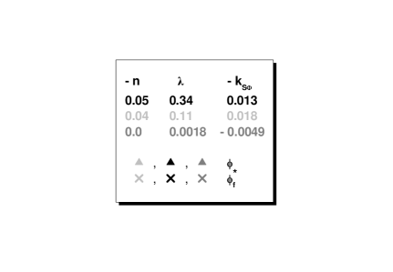
Figure 1: The inflationary potential $\widehat{V}_{\rm IG0}$ (gray, light gray and black line) as a function of $\phi$ for $n=0,-1/25,-1/20$, $\lambda=0.0013,0.11,0.34$ and $k_{S\Phi}\simeq 0.0045,-0.018,-0.013$. Values corresponding to $\phi_{\star}$ and $\phi_{\rm f}$ are also depicted.

4 Results

Confronting our inflationary scenario with the requirements above we can find its allowed parameter space. We here present our results for the two radically different cases: taking $n=0$ in Sec. 4.1 and $n<0$ in Sec. 4.2.

4.1 $n=0$ Case

We focus first on the form of Kähler potential induced by Eq. (14) with $n=0$. Our analysis in Sec. 4.1.1 presents some approximate expressions which assist us to interpret the numerical results exhibited in Sec. 4.1.2.

4.1.1 Analytic Results

Upon substitution of Eqs. (21) and (23b) into Eq. (27), we can extract the slow-roll parameters which determine the strength of the inflationary stage. Performing expansions about $\phi\simeq 0$, we can achieve approximate expressions which assist us to interpret the numerical results presented below. Namely, we find

$$\widehat{\epsilon}=\frac{(2+k_{S\Phi}c_{R}\phi^{4})^{2}}{3f_{W}^{2}}~{}~{}~{}\mbox{and}~{}~{}~{}\widehat{\eta}={1\over 3f_{W}^{2}}{\left(4+k_{S\Phi}c_{R}^{2}\phi^{6}+2c_{R}k_{S\Phi}\phi^{4}-1\right)}.$$ (32)

As it may be numerically verified, the termination of IGI is triggered by the violation of the $\epsilon$ criterion at $\phi=\phi_{\rm f}$, which does not decline a lot from its value for $k_{S\Phi}=0$. Namely we get

$$\widehat{\epsilon}\left(\phi_{\rm f}\right)=1\>\Rightarrow\>\phi_{\rm f}=\sqrt{1+2/\sqrt{3}/c_{R}}.$$ (33)

In the same approximation and given that $\phi_{\rm f}\ll\phi_{\star}$, $\widehat{N}_{\star}$ can be calculated via Eq. (26) with result

$$\widehat{N}_{\star}\simeq 3c_{R}\left({\phi_{\star}^{2}-\phi_{\rm f}^{2}}\right)/4\>\Rightarrow\>\phi_{\star}\simeq 2\sqrt{\widehat{N}_{\star}/3c_{R}}.$$ (34a)

Obviously, IGI with subplanckian $$\phi$$’s can be achieved if

$$\phi_{\star}\leq 1~{}~{}\Rightarrow~{}~{}c_{R}\geq 4\widehat{N}_{\star}/3\simeq 76$$ (34b)

for ${\widehat{N}}_{\star}\simeq 52$. Therefore we need relatively large $c_{R}$’s.

Replacing $\widehat{V}_{\rm IG0}$ from Eq. (21) in Eq. (28) we obtain

$$A_{\rm s}^{1/2}=\frac{2\lambda f_{W}^{2}(\phi_{\star})}{8\sqrt{2}\pi c_{R}^{2}\phi_{\star}^{2}(2+k_{S\Phi}c_{R}\phi_{\star}^{4})}\>\>\Rightarrow\>\>\lambda\simeq 2\pi\sqrt{2A_{\rm s}}c_{R}\left({3\over\widehat{N}_{\star}}+{8k_{S\Phi}\widehat{N}_{\star}\over 3c_{R}}\right)\cdot$$ (35)

Inserting finally Eq. (34a) into Eq. (29a) and (c) we can provide expressions for $n_{\rm s}$ and $r$. These are

$$n_{\rm s}\simeq 1-{2\over\widehat{N}_{\star}}\ +\ \frac{2{\widehat{N}}_{\star}}{3c_{R}}\frac{32k_{S\Phi}+27/{\widehat{N}}_{\star}^{3}}{12}~{}~{}~{}\mbox{and}~{}~{}~{}r\simeq{12\over\widehat{N}_{\star}^{2}}\ +\ 64\,{4k_{S\Phi}^{2}\widehat{N}_{\star}^{2}\over 9c_{R}^{2}}\cdot$$ (36)

Therefore, a clear dependence of $n_{\rm s}$ and $r$ on $k_{S\Phi}$ arises, with the first one being much more efficient. This depedence does not exist within no-scale SUGRA since $k_{S\Phi}$ vanishes by definition – see Eq. (15).

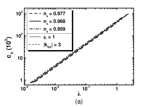
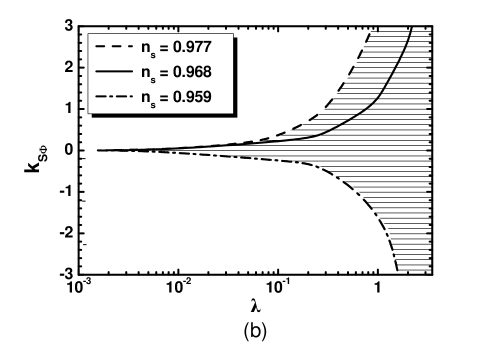
Figure 2: Allowed (hatched) regions in the $\lambda-c_{R}$ plane (${\sf\footnotesize a}$) and $\lambda-k_{S\Phi}$ plane (${\sf\footnotesize b}$) for $k_{S}=k_{\Phi}=0.5$. The conventions adopted for the various lines are also shown.

4.1.2 Numerical Results

With fixed $k_{\sf NS}$ and $T_{\rm rh}$ – see Secs 2 and 3.2 – this inflationary scenario depends on the parameters:

$$\lambda,\>c_{R},\>k_{S},\>k_{S\Phi},\>\>\mbox{and}~{}~{}~{}k_{\Phi}.$$ (37)

Our results are independent of $k_{S}$, provided that $\widehat{m}_{s}^{2}>0$ – see in Table 1. The same is also valid for $k_{\Phi}\simeq 1\ll c_{R}$ – see Eq. (20b). We therefore set $k_{S}=k_{\Phi}=0.5$. Besides these values, in our numerical code, we use as input parameters $c_{R},~{}k_{S\Phi}$ and $\phi_{\star}$. For every chosen $c_{R}\geq 1$, we restrict $\lambda$ and $\phi_{\star}$ so that the conditions Eqs. (26), (28) and (31) are satisfied. By adjusting $k_{S\Phi}$ we can achieve $n_{\rm s}$’s in the range of Eq. (30). Our results are displayed in Fig. 2-(a) and (b) where we delineate the hatched regions allowed by the restrictions of Sec. 3.2 in the $\lambda-c_{R}$ [$\lambda-k_{S\Phi}$] plane. The conventions adopted for the various lines are also shown. In particular, the dashed [dot-dashed] lines correspond to $n_{\rm s}=0.977$ [$n_{\rm s}=0.959$], whereas the solid (thick) lines are obtained by fixing $n_{\rm s}=0.968$ – see Eq. (30). Along the thin line, which provides the lower bound for the regions presented in Fig. 2, the constraint of Eq. (31b) is saturated. At the other end, the allowed regions terminate along the dotted line where $|k_{S\Phi}|=3$, since we expect $k_{S\Phi}$ values of order unity to be natural. From Fig. 2-(a) we see that $c_{R}$ remains almost proportional to $\lambda$ and for constant $\lambda$, $c_{R}$ increases as $n_{\rm s}$ decreases. From Fig. 2-(b) we remark that $k_{S\Phi}$ is confined close to zero for $n_{\rm s}=0.968$ and $\lambda<0.16$ or $\phi_{\star}>0.1$ – see Eq. (34a). Therefore, a degree of tuning (of the order of $10^{-2}$) is needed in order to reproduce the experimental data of Eq. (30a). On the other hand, for $\lambda>0.16$ (or $\phi_{\star}<0.1$), $k_{S\Phi}$ takes quite natural (of order one) negative values – consistently with Eq. (36).

More explicitly, for $n_{\rm s}=0.968$ and $\widehat{N}_{\star}\simeq 52$ we find:

$$78\lesssim c_{R}\lesssim 10^{5}~{}~{}~{}\mbox{with}~{}~{}~{}1.9\cdot 10^{-3}\lesssim\lambda\lesssim 2.35~{}~{}~{}\mbox{and}~{}~{}~{}0.005\lesssim k_{S\Phi}\lesssim 3\,.$$ (38)

Note that the former data dictated $k_{S\Phi}<0$ since the central $n_{\rm s}$ was lower [4]. Also we obtain $-7.8\lesssim{a_{\rm s}/10^{-4}}\lesssim-7.4$ and $r\simeq 4.4\cdot 10^{-3}$ which lie within the allowed ranges of Eq. (30). On the other hand, the results within no-scale SUGRA are much more robust since the $k_{S\Phi}$ (and $k_{\Phi}$) dependence collapses – see Eq. (15). Indeed, no-scale SUGRA predicts identically $n_{\rm s}\simeq 0.963,~{}a_{\rm s}=-6.5\cdot 10^{-4}$ and $r=4\cdot 10^{-3}$ which are perfectly compatible with the data [6, 7] although with low enough $r$.

4.2 $n<0$ Case

Following the strategy of the previous section, we present below first some analytic results in Sec. 4.2.1, which provides a taste of the numerical findings exhibited in Sec. 4.2.2.

4.2.1 Analytic Results

Plugging Eqs. (21) and (23b) into Eq. (27) and taking $k_{\Phi}\simeq 0$, we obtain the following approximate expressions for the slow-roll parameters

$$\widehat{\epsilon} =\frac{(2+3n-3nc_{R}\phi^{2}+(1+3n)k_{S\Phi}c_{R}\phi^{4})^{2}}{3(1+n)f_{S\Phi}^{2}f_{W}^{2}}~{}~{}~{}\mbox{and}~{}~{}~{}\widehat{\eta}=\frac{1}{3(1+n)f_{S\Phi}^{2}f_{W}^{2}}\times$$ (39)

$$\times 2\Big{[}\phi^{2}\Big{(}k_{S\Phi}\left(\phi^{2}\left(6c_{R}+c_{R}^{2}\phi^{2}+k_{S\Phi}c_{R}^{2}\phi^{4}\right)-11\right)-2c_{R}\Big{)}+9n^{2}f_{S\Phi}^{2}f_{W}^{2}$$

$$+ 4+6nf_{S\Phi}f_{W}\left(2+k_{S\Phi}\phi^{2}(c_{R}\phi^{2}-3)\right)\Big{]}\,.$$

Taking the limit of the expressions above for $k_{S\Phi}\simeq 0$ we can analytically solve the condition in Eq. (27) w.r.t $\phi$. The results are

$${\phi_{1\rm f}}=\sqrt{\frac{3(1-n)+2\sqrt{3(1+n)}}{3(1+n)c_{R}}}~{}~{}~{}\mbox{and}~{}~{}~{}{\phi_{2\rm f}}=\sqrt{\frac{1-9n+\sqrt{16+21n(3n-1)}}{3(1+n)c_{R}}}\,\cdot$$ (40)

The end of IGI mostly occurs at $\phi_{\rm f}=\phi_{1\rm f}$ because this is mainly the maximal value of the two solutions above. Since $\phi_{\rm f}\ll\phi_{\star}$, we can estimate $\widehat{N}_{\star}$ through Eq. (26) neglecting $\phi_{\rm f}$. Our result is

$$\widehat{N}_{\star}\simeq(1+n)\frac{3n\ln\phi_{\star}+\ln\left(2+3n-3c_{R}n\phi_{\star}^{2}\right)}{|n|(2+3n)}\cdot$$ (41a)

Ignoring the first term in the last equality and solving w.r.t $$\phi_{\star} \phi_{\star}$$ we extract as follows – cf. Ref. [4, 10]:

$$\phi_{\star}\simeq\sqrt{(2-e_{n})/3nc_{R}}~{}~{}~{}\mbox{with}~{}~{}~{}e_{n}=e^{-n(2+3n)\widehat{N}_{\star}/(1+n)}\,.$$ (41b)

Although a radically different dependence of $$\phi_{\star} \widehat{N}_{\star} \phi_{\star} c_{R}$$ on arises compared to the model of Sec. 4.1 – cf. Eq. (34a) – can again remain subplanckian for large ’s. Indeed,

$$\phi_{\star}\leq 1~{}~{}~{}\Rightarrow~{}~{}~{}c_{R}\geq(2-e_{n})/3n\,.$$ (41c)

On the other hand, $\widehat{\phi}_{\star}$ remains transplanckian, since plugging Eq. (41b) into Eq. (24) we find

$$\widehat{\phi}_{\star}\simeq-\sqrt{3(1+n)/2}\left({4(2+3n)\widehat{N}_{\star}/(1+n)}+\ln 3|n|\right),$$ (42)

which gives $\widehat{\phi}_{\star}=7-10$ for $\widehat{\phi}_{\rm c}=0$ and $n=-(0.03-0.05)$ – independently of $c_{R}$. Despite this fact, our construction remains stable under possible corrections from non-renormalizable terms in $\Omega_{\rm H}$ since these are expressed in terms of initial field $\Phi$, and can be harmless for $|\Phi|\leq 1$.

Upon substitution of Eq. (41b) into Eq. (28) we end up with

$$\lambda\simeq\frac{4\pi\sqrt{2c_{R}A_{\rm s}}e_{n}^{3n/2}(e_{n}-2)(k_{S\Phi}(1+3n)(e_{n}-2)^{2}+9n^{2}c_{R}e_{n})}{3|n|^{(3n+1)/2}\sqrt{(1+n)(k_{S\Phi}(e_{n}-2)-3nc_{R}}}\cdot$$ (43)

We remark that $\lambda$ depends not only on $c_{R}$ and $k_{S\Phi}$ as in Eq. (35) but also on $n$. Inserting Eq. (41b) into Eq. (39), employing then Eq. (29a) and expanding for $c_{R}\gg 1$ we find

$$n_{\rm s}=\frac{(e_{n}-2)^{2}+n(e_{n}-2)(e_{n}+12)-6n^{2}e_{n}^{2}}{(1+n)(e_{n}+3n-2)^{2}}\ +\ 4k_{S\Phi}\,e_{n}\,\frac{e_{n}(4-(1+3m)e_{n})-4}{9n(1+n)(e_{n}+3n-2)^{2}c_{R}}\cdot$$ (44a)

Following the same steps, from Eq. (29c) we find

$$r=16\left(\frac{3n^{2}e_{n}^{2}}{(1+n)(e_{n}+3n-2)^{2}}\ +\ 2k_{S\Phi}e_{n}\frac{4+(e_{n}-3ne_{n}-4)e_{n}}{3(1+n)(e_{n}+3n-2)^{2}c_{R}}\right)\cdot$$ (44b)

From the above expressions we see that primarily $|n|\neq 0$ and secondarily $n<0$ help to sizably increase $r$. Given that $e_{n}\gg 1$, $n_{\rm s}$ is close to unity as can be infered by the first ratio in the right-hand side of Eq. (44a). Any increase of $n_{\rm s}$ due to the existence $|n|\neq 0$ can be balanced by a choise of $k_{S\Phi}<0$. Note that the second term in Eq. (44a) is less suppressed w.r.t the second term in Eq. (44b) since $c_{R}\gg 1$ is multiplied by $n\ll 1$.

4.2.2 Numerical Results

Besides the free parameters shown in Eq. (37) we have also here $n$, which is constrained to negative values. Using the reasoning explained in Sec. 4.1.2 we set $k_{\Phi}=0.5$. On the other hand, $\widehat{m}_{s}^{2}$ can become positive with $k_{S}$ lower than the value used in Sec. 4.1.2 since positive contributions from $n<0$ arises here – see Table 1. Moreover, if $k_{S}$ takes a value of order unity $\widehat{m}_{s}^{2}$ grows more efficiently than in the case with $n=0$, rendering thereby the RCs in Eq. (25) sizeable for very large $c_{R}$ values ($\sim 10^{5}$). To avoid such dependence of the model predictions on the RCs, we use $k_{S}$ values lower than those used in Sec. 4.1.2. Thus, we set $k_{S}=0.05$ throughout. As in the previous case, Eqs. (26), (28) and (31) assist us to restrict $\lambda$ (or $c_{R}\geq 1$) and $\phi_{\star}$. By adjusting $n$ and $k_{S\Phi}$ we can achieve not only $n_{\rm s},a_{\rm s}$ and $r$ values in the range of Eq. (30) but also $r$’s close to the central value reported in Ref. [7].

Confronting the parameters with Eqs. (26), (28), (30a, b) and (31) we depict the allowed (hatched) regions in the $\lambda-c_{R}$, $\lambda-k_{S\Phi}$, $\lambda-r$ and $\lambda-a_{\rm s}$ planes for $n=-1/30$ (gray lines and hatched regions), $n=-1/25$ (light gray lines and hatched regions), $n=-1/20$ (black lines and hatched regions) in Fig. 3-(a), (b), (c) and (d) respectively. Note that the conventions adopted for the various lines are identical with those used in Fig. 2 – i.e., the dashed, solid (thick) and dot-dashed lines correspond to $n_{\rm s}=0.977,0.968$ and $0.959$ respectively, whereas along the thin (solid) lines the constraint of Eq. (31b) is saturated. The perturbative bound on $\lambda$ limits the various regions at the other end.

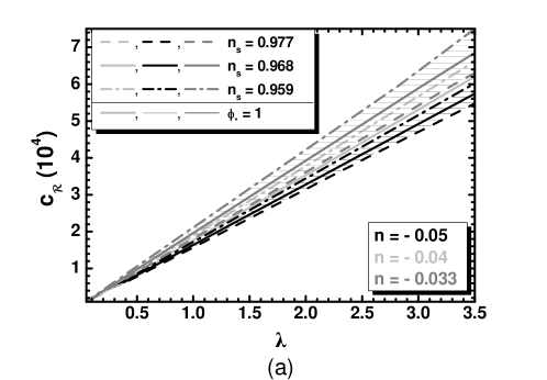
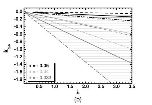
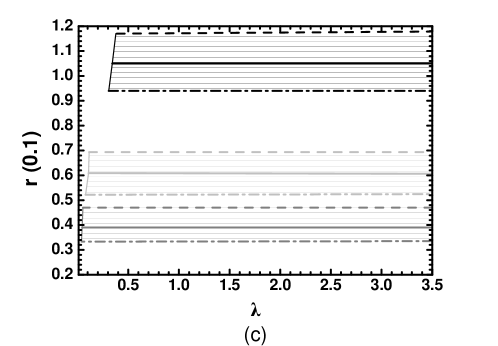
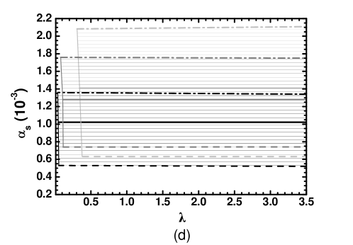
Figure 3: Allowed (hatched) regions in the $\lambda-c_{R}$ (a), $\lambda-k_{S\Phi}$ (b), $\lambda-r$ (c), $\lambda-a_{\rm s}$ (d) plane for $k_{S}=0.1$, $k_{\Phi}=0.5$ and $n=-0.033$ (gray lines and hatched regions), $n=-0.04$ (light gray lines and hatched regions), $n=-0.05$ (black lines and hatched regions). The conventions adopted for the type and color of the various lines are also shown in the label of panel (a).

From Fig. 3-(a) we remark that $c_{R}$ remains almost proportional to $\lambda$ but the dependence on $k_{S\Phi}$ is stronger than that shown in Fig. 2-(a). Also, as $|n|$ increases, the allowed areas are displaced to larger $\lambda$ and $c_{R}$ values in agreement with Eq. (41c) – cf. Fig. 2. Similarly, the allowed $k_{S\Phi}$’s move to larger values as $|n|$ and/or $n_{\rm s}$ increases. For fixed $n_{\rm s}$, increasing $c_{R}$ entails a decrease of $k_{S\Phi}$ in accordance with Eq. (44a). Finally, from Fig. 3-(c) and (d) we conclude that employing $|n|\gtrsim 0.01$, $r$ and $a_{\rm s}$ increase w.r.t their values for $n=0$ – see results below Eq. (38). As a consequence, for $n\simeq-(0.03-0.05)$, $r$ enters the observable region. On the other hand, $a_{\rm s}$ although one order larger than its value for $n=0$ remains sufficiently low; it is thus consistent with the fitting of data with the standard $\Lambda$CDM$+r$ model – see Eq. (30). As anticipated below Eq. (44b), the resulting $r$’s depend only on the input $n$ and $k_{S\Phi}$ (or $n_{\rm s}$), and are independent of $\lambda$ (or $c_{R}$). The same behavior is also true for $a_{\rm s}$. It is worth noticing that the existence of $k_{S\Phi}\neq 0$ is imperative for the viability of our scheme. More explicitly, for $n_{\rm s}=0.968$ and ${\widehat{N}}_{\star}\simeq 55-57$ we find:

$$0.09\lesssim{c_{R}\over 10^{4}}\lesssim 6.9~{}~{}~{}\mbox{with}~{}~{}~{}0.045\lesssim\lambda\lesssim 3.5~{}~{}~{}\mbox{and}~{}~{}~{}0.18\lesssim-{k_{S\Phi}\over 0.1}\lesssim 10.4\,~{}~{}~{}(n=-0.033);~{}~{}~{}~{}~{}~{}$$ (45a)

$$0.19\lesssim{c_{R}\over 10^{4}}\lesssim 6.7~{}~{}~{}\mbox{with}~{}~{}~{}0.11\lesssim\lambda\lesssim 3.5~{}~{}~{}\mbox{and}~{}~{}~{}0.18\lesssim-{k_{S\Phi}\over 0.1}\lesssim 6.3\,~{}~{}~{}(n=-0.04);~{}~{}~{}~{}~{}~{}$$ (45b)

$$0.56\lesssim{c_{R}\over 10^{4}}\lesssim 6.1~{}~{}~{}\mbox{with}~{}~{}~{}0.34\lesssim\lambda\lesssim 3.5~{}~{}~{}\mbox{and}~{}~{}~{}0.13\lesssim-{k_{S\Phi}\over 0.1}\lesssim 1.45\,~{}~{}~{}(n=-0.05).~{}~{}~{}~{}~{}~{}~{}~{}~{}~{}~{}~{}\>$$ (45c)

In these regions we obtain

$${r\over 0.1}=0.4,0.6,1.05~{}~{}~{}\mbox{and}~{}~{}~{}{a_{\rm s}\over 0.001}=1,1.3,1.4~{}~{}~{}\mbox{for}~{}~{}~{}-{n\over 0.01}=3.3,4,5$$ (46)

respectively. It is impressive that the observable $r$’s above are achieved with subplanckian $\phi$’s. However, this fact does not contradict to the Lyth bound [13], since this is applied to the (totally auxiliary) EF inflaton $\widehat{\phi}$ which remains transplanckian– see Eq. (42).

5 Effective Cut-off Scale

An outstanding trademark of IGI is that it is unitarity-safe [4, 2, 3], despite the fact that its implementation with subplanckian $\phi$’s – see Eqs. (34b) and (41c) – requires relatively large $c_{R}$’s. To show this, we below extract the UV cut-off scale, $\Lambda_{\rm UV}$, of the effective theory first in the JF – see Sec. 5.1 – and then in the EF – see Sec. 5.2.

5.1 Jordan Frame Computation

If we expand $g_{\mu\nu}$ about the flat spacetime metric $\eta_{\mu\nu}$ and $\phi$ about its v.e.v as follows

$$g_{\mu\nu}\simeq\eta_{\mu\nu}+{h_{\mu\nu}}~{}~{}~{}\mbox{and}~{}~{}~{}\phi=\langle{\phi}\rangle+\delta\phi~{}~{}~{}\mbox{with}~{}~{}~{}\langle{\phi}\rangle=1/\sqrt{c_{R}}$$ (47)

– where $h^{\mu\nu}$ is the graviton –, the lagrangian corresponding to the two first terms in the right-hand side of ${\sf S}$ in Eq. (11) for ${\alpha}=\Phi$ takes the form – cf. Ref. [14]:

$$\delta{\cal L} = -{\langle{f_{R}}\rangle\over 4}{F}_{\rm EH}\left(h^{\mu\nu}\right)+\frac{\langle{F_{\rm K}}\rangle}{2}\partial_{\mu}\delta\phi\partial^{\mu}\delta\phi+\left(\langle{f_{R,\phi}}\rangle\delta\phi+\frac{1}{2}\langle{f_{R,\phi\phi}}\rangle\delta\phi^{2}+\cdots\right)F_{R}$$ (48)

$$= -{1\over 8}F_{\rm EH}\left(\bar{h}^{\mu\nu}\right)+\frac{1}{2}\partial_{\mu}\overline{}\delta\phi\partial^{\mu}\overline{}\delta\phi+\Lambda_{\rm UV}^{-1}\overline{}\delta\phi^{2}\,\Box\bar{h}\,,$$

where the functions $F_{\rm EH}$ and $F_{R}$ related to the the linearized Einstein-Hilbert part of the lagrangian, read

$${F}_{\rm EH}\left(h^{\mu\nu}\right)=h^{\mu\nu}\Box h_{\mu\nu}-h\Box h+2\partial_{\rho}h^{\mu\rho}\partial^{\nu}h_{\mu\nu}-2\partial_{\nu}h^{\mu\nu}\partial_{\mu}h~{}~{}~{}\mbox{and}~{}~{}~{}F_{R}\left(h^{\mu\nu}\right)=\Box h-\partial_{\mu}\partial_{\nu}h^{\mu\nu}\,$$ (49)

with $h=h^{\mu}_{\mu}$. Also $F_{\rm K}$ along the trajectory in Eq. (17) is calculated to be

$$F_{\rm K}=\Omega_{\Phi{\Phi^{*}}}-\frac{n\Omega_{\Phi}\Omega_{\Phi^{*}}}{(1+n)\Omega}=\frac{k_{\sf NS}}{1+n}+6nc_{R}\,\cdot$$ (50)

Moreover, $\bar{h}_{\mu\nu}$ and $\overline{}\delta\phi$ are the JF canonically normalized fields defined by the relations

$$\overline{}\delta\phi=\sqrt{\frac{\langle{f_{R}}\rangle}{\langle{\bar{f}_{R}}\rangle}}\delta\phi~{}~{}~{}\mbox{and}~{}~{}~{}\bar{h}_{\mu\nu}=\sqrt{\langle{f_{R}}\rangle}\,h_{\mu\nu}+\frac{\langle{f_{R,\phi}}\rangle}{\sqrt{\langle{f_{R}}\rangle}}\eta_{\mu\nu}\delta\phi~{}~{}~{}\mbox{with}~{}~{}~{}\bar{f}_{R}=F_{\rm K}f_{R}+\frac{3}{2}f_{R,\phi}^{2}\,.$$ (51)

Finally, $\Lambda_{\rm UV}$ in Eq. (48) is the JF UV cut-off scale since it controls the strength of the $\delta\phi-\delta\phi$ scattering process via $s$-channel $h^{\mu\nu}$ exchange. It is determined via the relation

$$\Lambda_{\rm UV}=\frac{2\langle{\bar{f}_{R}}\rangle}{\sqrt{\langle{f_{R}}\rangle}\langle{f_{R,\phi\phi}}\rangle}\simeq\frac{6(1+n)}{\sqrt{1-{k_{\sf NS}\over 6(1+n)c_{R}}}}\,\cdot$$ (52)

For the estimations above we make use of Eqs. (47) and (50). Since the dangerous factor $c_{R}^{-1}$ included in $\langle{f_{R,\phi\phi}}\rangle$ is eliminated in Eq. (52), the theory can be characterized as unitarity-safe.

5.2 Einstein Frame Computation

Alternatively, $\Lambda_{\rm UV}$ can be determined in EF, following the systematic approach of Ref. [15]. At the SUSY vacuum in Eq. (5), the EF (canonically normalized) inflaton is found via Eq. (24) to be

$$\widehat{\delta\phi}=\langle{J}\rangle\delta\phi~{}~{}~{}\mbox{with}~{}~{}~{}\langle{J}\rangle\simeq\sqrt{6(1+n)c_{R}}\,.$$ (53)

The fact that $\widehat{\delta\phi}$ does not coincide with $\delta\phi$ at the vacuum of the theory – contrary to the standard Higgs non-minimal inflation [16] – ensures that our models are valid up to $m_{\rm P}=1$. To show it, we write ${\sf S}$ in Eq. (6) along the path of Eq. (17) as follows

$${\sf S}=\int d^{4}x\sqrt{-\widehat{\mathfrak{g}}}\left(-\frac{1}{2}\widehat{R}+\frac{1}{2}\,J^{2}\dot{\phi}^{2}-\widehat{V}_{\rm IG0}+\cdots\right),$$ (54)

where the ellipsis represents terms irrelevant for our analysis; $J$ and $\widehat{V}_{\rm IG0}$ are given by Eqs. (23b) and (21) respectively. We first expand $J^{2}\dot{\phi}^{2}$ about $\langle{\phi}\rangle$ in terms of $\widehat{\delta\phi}$ in Eq. (53) and we arrive at the following result

$$J^{2}\dot{\phi}^{2}=\left(1-\sqrt{\frac{2}{3(1+n)}}{\widehat{\delta\phi}}+\frac{\widehat{\delta\phi}^{2}}{2(1+n)}-\sqrt{\frac{2}{3(1+n)^{3}}}\frac{\widehat{\delta\phi}^{3}}{3}+\cdots\right)\dot{}\widehat{\delta\phi}^{2}.$$ (55a)

The expansion corresponding to $$\widehat{V}_{\rm IG0} k_{S\Phi}\simeq 0 k_{\Phi}\simeq 0$$ in Eq. (21) with and includes the terms:

$$\widehat{V}_{\rm IG0}=\frac{\lambda^{2}\widehat{\delta\phi}^{2}}{6c_{R}^{4}(1+n)}\left(1+\frac{\widehat{\delta\phi}}{\sqrt{6(1+n)^{3}}}+\frac{\widehat{\delta\phi}^{2}}{24(1+n)^{2}}-\cdots\right)\cdot~{}~{}~{}$$ (55b)

From Eqs. (55a) and (55b) we conclude that $\Lambda_{\rm UV}=1$, in agreement with our analysis in Sec. 5.1.

6 Conclusions

We updated the analysis of IGI introduced in Ref. [4], in the view of the combined recent analysis of the Planck and Bicep2/Keck Array results [6, 7]. These inflationary models are tied to a superpotential, which realizes easily the idea of induced gravity, and a logarithmic Kähler potential, which includes all the allowed terms up to the fourth order in powers of the various fields – see Eq. (14). We also allowed for deviations from the prefactor $(-3)$ multiplying the logarithm of the Kähler potential, parameterizing it by a factor $(1+n)$. The models are totally defined imposing two global symmetries – a continuous $R$ and a discrete $\mathbb{Z}_{2}$ symmetry – in conjunction with the requirement that the original inflaton takes subplanckian values.

In the case of no-scale SUGRA, thanks to the underlying symmetries, the inflaton is not mixed with the accompanying non-inflaton field in the Kähler potential. As a consequence, the model predicts $n_{\rm s}\simeq 0.963$, $a_{\rm s}\simeq-0.00065$ and $r\simeq 0.004$, in excellent agreement with the current Planck data. Beyond no-scale SUGRA, for $n=0$, we showed that $n_{\rm s}$ spans the entire allowed range in Eq. (30a) by conveniently adjusting the coefficient $k_{S\Phi}$. In addition, for $n\simeq-(0.03-0.05)$, $r$ becomes compatible with the 1-$\sigma$ domain of the joint analysis of Planck and Bicep2/Keck Array data and accessible to the ongoing measurements with negligibly small $a_{\rm s}$. In this last case a mild tuning of $k_{S}$ to values of order $0.05$ is adequate so that the one-loop RCs remain subdominant. Moreover, in all cases, the corresponding effective theory is valid up to the Planck scale.