STRUCTURE FUNCTIONS OF MANY-BOSON
SYSTEM WITH REGARD FOR DIRECT THREE-
AND FOUR-PARTICLE CORRELATIONS

Abstract

On the basis of the expression for the density matrix of interacting Bose particles in the coordinate representation with regard for the direct three- and four-particle correlations [I.O.  Vakarchuk and O.I.  Hryhorchak, J.  Phys.  Stud.  3, 3005 (2009)], the two-, three-, and four-particle structure factors of liquid ⁴He in a wide temperature interval were calculated in the approximation ‘‘one sum over the wave vector’’.  In the low-temperature limit, the expression obtained for the two-particle structure factor transforms into the well-known one.  In the high-temperature limit, the expressions for the two-, three-, and four-particle structure factors are reduced to those for the ideal Bose gas.  The results obtained can be applied to calculations of the thermodynamic functions of liquid ⁴He and to the determination of the temperature dependence of the first-sound velocity in a many-boson system.

1 Introduction

The researches of structure functions play an important role in studying the Bose and Fermi systems, because the results obtained theoretically can be compared directly with experimental data.  The central role in the structural researches of those systems belongs to the total scattering cross-section, which is called the dynamic structure factor.  This parameter makes it possible to determine both the spatial structure of the substance and the structure of its energy spectrum [1,​ 2].  With its help, as well as with the help of its derivatives, a lot of different systems are studied today, e.g., the Bose gas in a trap [3], liquid ⁴He [4] and ³He [5] in two dimensions, solid ³He [6], thin films [7], Lennard-Jones rarefied gas [8], superfluid helium [9], parahydrogen [10], models with turbulence [11], and so forth.

Besides the dynamic structure factor, not less important is its zeroth moment or the static structure factor, which has been measured a lot of times in a wide temperature interval.  The researches were carried out at the saturated vapor pressure within the neutron [12] and X-ray [13] diffraction methods.  Experimental works on the structure factor measurement were analyzed, e.g., in work [14], where corrections were also proposed in order to coordinate results of various authors.  The Monte-Carlo method was applied to study the region around the structure factor peak in a Bose condensate, and the peak was shown to locate higher than the theoretical value obtained in the framework of the low-density approximation [15].  The contribution of three-particle correlations to the structure factor of liquid ⁴He was found in work [16], and a procedure of calculation of the effective pair potential on the basis of experimental data obtained for the structure factor and with the help of the Monte-Carlo simulation scheme was proposed in work [17].  Among structure functions, we also mention the pair correlation function, which is one of the key quantities characterizing the coherent properties of a Bose condensate [18].

In this work, we aimed at finding not only the pair structure factor, but also expressions for the three- and four-particle structure factors in the approximation ‘‘one sum over the wave vector’’.  This result should help us, in turn, to simplify calculations of the thermodynamic functions of a Bose system in the approximation “two sums over the wave vector” and to facilitate the solution of the still unsolved task to describe such a system as liquid ⁴He in a wide temperature interval and, especially, in a vicinity of the $\lambda$-transition.

The structural properties of liquid ⁴He at low temperatures have been discussed for a long time in the framework of the collective variable approach [19,​ 20,​ 21,​ 22,​ 23].  However, a theoretical calculation of the pair structure factor in a wide temperature interval has been carried out only recently in work [24], by taking advantage of the averaging with the density matrix of interacting Bose particles.  Later on, the structure functions in a wide temperature interval were also described in other works [25].  However, the authors of the cited works calculated the average values in the framework of the density matrix approach and in the pair correlation approximation, so that the pair structure factor was obtained in the same approximation.  The agreement with experimental data for the pair structure factor [12,​ 13,​ 26] is good in this case, but incomplete, because, as is known, the contribution of many-particle correlations to the observed quantities of a many-boson system can turn out rather substantial [27,​ 28,​ 22].

In works [25], the irreducible two-, three-, and four-particle structure factors, as well as the pair distribution function, were calculated in a wide temperature interval making allowance for only the indirect three- and four-particle correlations.  The obtained theoretical results can be improved by taking direct correlations into account as well.  However, in this case, the indicated quantities have to be calculated with the density matrix containing not only the pair, but also three- and four-particle direct correlations.  This task is a purpose of this work.  In our calculations, we will base on the approaches proposed in our earlier works [29,​ 30] and the results obtained there; in particular, these are the expressions for the density matrix and the partition function for a many-boson system in a wide temperature interval and the methods of their calculation in the approximation ‘‘two sums over the wave vector’’.

An important feature of this work is a graphic presentation of the results obtained.  As a rule, numerical calculations are carried out for this purpose.  The input data at such calculations include experimental results for the structure factor extrapolated to the absolute zero temperature.  The general scheme of speculations on this topic and the corresponding results can be found in work [31].  Continuing the issue of numerical calculations, it is worth paying attention to work [32], where the interatomic interaction potentials were restored on the basis of experimental data (as was done in work [31]), and the thermodynamic and structural properties of ⁴He were studied.

The numerical calculation of the pair structure factor was carried out taking the effective mass into account.  The expression for the latter was given in work [33].  A necessity of its introduction was substantiated in work [25].

The expression obtained for the two-particle structure factor transforms into an already found one for the low-temperature limit [21].  In the high-temperature limit, the expression for the two-, three-, and four-particle structure factors are reduced to the corresponding structure factors of the ideal Bose gas.  The two-particle structure factor obtained in the approximation “one sum over the wave vector” also opens a way to finding the temperature dependence of the first-sound velocity in liquid ⁴He and to comparing it with experimental data.

2 $n$-Particle Structure
Factors for a Many-Boson System

According to the definition, the $n$-particle structure factor equals

$$S^{(n)}(\rho_{{\mathbf{q}}_{1}},...,\rho_{{\mathbf{q}}_{n}})=N^{n/2-1}\langle\rho_{{\mathbf{q}}_{1}}...\rho_{{\mathbf{q}}_{n}}\rangle,$$

where $N$ is the number of particles, $\rho_{q}=$$=\frac{1}{\sqrt{N}}\sum_{j=1}^{N}e^{-i\mathbf{{qr_{j}}}}$ are collective variables, and the notation $\langle...\rangle$ means the averaging with the density matrix of interacting Bose particles.  In the calculations to follow, the density matrix in the approximation “two sums over the wave vector” with the factorized density matrix of the ideal Bose gas will be used.  This approximation involves the direct three- and four-particle correlations, and the matrix itself looks like

$$R(\rho|\rho^{\prime})=R_{N}^{0}(r|r^{\prime})P_{pr}(\rho|\rho^{\prime})P(\rho|\rho^{\prime}),$$

where $R_{N}^{0}(r|r^{\prime})$ is the density matrix for noninteracting Bose particles, $P_{pr}(\rho|\rho^{\prime})$ a factor taking into account pair correlations, and $P(\rho|\rho^{\prime})$ a factor taking the direct three- and four-particle correlations into account.  In particular,

$$R_{N}^{0}(r^{\prime}|r)=\frac{1}{N!}\left(\!\frac{m}{2\pi\beta\hbar^{2}}\!\right)^{\!\!3N/2}\times$$

$$\times\sum\limits_{Q}\exp\left[-\frac{m}{2\beta\hbar^{2}}\sum\limits_{j=1}^{N}(r_{j}^{\prime}-r_{Q_{j}})^{2}\right]\!\!,$$

where the summation over $Q$ means the summation over all permutations of particle coordinates.  The factor which makes allowance for pair correlations looks like [34]

$$P_{pr}(\rho|\rho^{\prime})=\exp\biggl{[}b_{0}+\sum_{\mathbf{q}\neq 0}b_{1}(q){\rho_{\mathbf{q}}}^{\prime}\rho_{-\mathbf{q}}\,-$$

$$-\,\frac{1}{2}\sum_{\mathbf{q}\neq 0}b_{2}(q)\rho_{\mathbf{q}}\rho_{-\mathbf{q}}\biggr{]}\!,$$

where

$$b_{0}=-\beta E_{0}+\frac{1}{2}\sum_{{\mathbf{q}}\neq 0}\ln\left[\frac{\alpha_{q}\tanh\left(\!\frac{\beta E_{q}}{2}\!\right)}{\tanh\left(\!\frac{\beta\varepsilon_{q}}{2}\!\right)}\right]+$$

$$+\sum_{{\mathbf{q}}\neq 0}\ln\left(\!\frac{1-e^{-\beta\varepsilon_{q}}}{1-e^{-\beta E_{q}}}\!\right)\!\!,$$

$$b_{1}(q)=\frac{1}{2}\left(\!\frac{\alpha_{q}}{\sinh(\beta E_{q})}-\frac{1}{\sinh(\beta\varepsilon_{q})}\!\right)\!\!,$$

$$b_{2}(q)=\frac{1}{2}\left(\alpha_{q}\coth(\beta E_{q})-\coth(\beta\varepsilon_{q})\right)\!,$$

$$\alpha_{q}=\sqrt{1+{\frac{2N}{V}\nu_{q}}\left/\frac{\hbar^{2}q^{2}}{2m}\right.},$$

$$E_{q}=\varepsilon_{q}\alpha_{q}=\frac{\hbar^{2}q^{2}}{2m}\alpha_{q},$$

$$\nu_{q}=\int e^{-i\mathbf{qr}}\Phi(r)d\mathbf{r}$$

is the Fourier coefficient of the pair interaction energy between particles, and $\beta=1/T$ is the inverse temperature.  An expression for $P(\rho|\rho^{\prime})$ was presented in work [29].  Its simplified version can be found in Appendix 1.  As a result, we obtain

$$\langle\rho_{{\mathbf{q}}_{1}}...\rho_{{\mathbf{q}}_{n}}\rangle=\frac{1}{Z}\int d{\mathbf{r}}_{1}...\int d{\mathbf{r}}_{N}\,\times$$

$$\times\,R_{N}^{0}(r|r)P_{pr}(\rho|\rho)P(\rho|\rho)\rho_{{\mathbf{q}}_{1}}...\rho_{{\mathbf{q}}_{n}}=$$

$$=\frac{1}{Z}\int d{\mathbf{r}}_{1}...\int d{\mathbf{r}}_{N}R_{N}^{0}(r|r)\rho_{{\mathbf{q}}_{1}}...\rho_{{\mathbf{q}}_{n}}\,\times$$

$$\times\,\exp\Bigg{[}b_{0}-\frac{1}{2}\sum_{\mathbf{q}\neq 0}\lambda_{q}\rho_{\mathbf{q}}\rho_{-\mathbf{q}}+C_{0}+2\sum_{\mathbf{q}\neq 0}C_{2}({\mathbf{q}})\rho_{\mathbf{q}}\rho_{-{\mathbf{q}}}\,+$$

$$+\frac{2}{\sqrt{N}}\mathop{\sum_{\mathbf{q}_{1}\neq 0}\sum_{\mathbf{q}_{2}\neq 0}\sum_{\mathbf{q}_{3}\neq 0}}\limits_{{\mathbf{q}}_{1}+{\mathbf{q}}_{2}+{\mathbf{q}}_{3}=0}C_{3}({\mathbf{q}}_{1},{\mathbf{q}}_{2},{\mathbf{q}}_{3})\rho_{\mathbf{q}_{1}}\rho_{\mathbf{q}_{2}}\rho_{\mathbf{q}_{3}}\,+$$

$$+\,\frac{2}{N}\sum\limits_{\mathbf{q}_{1}\neq 0}\sum\limits_{\mathbf{q}_{2}\neq 0}C_{4}(\mathbf{q}_{1},\mathbf{q}_{2})\rho_{\mathbf{q}_{1}}\rho_{-\mathbf{q}_{1}}\rho_{\mathbf{q}_{2}}\rho_{-\mathbf{q}_{2}}\Bigg{]}\!,$$ (1)

where

$$\lambda_{q}=2b_{2}(q)-b_{1}(q)=$$

$$=\alpha_{q}\tanh\left(\!\frac{\beta}{2}E_{q}\!\right)-\tanh\left(\!\frac{\beta}{2}\varepsilon_{q}\!\right)\!\!.$$

Explicit expressions for the quantities $C_{0}$, $C_{2}({\mathbf{q}}_{1})$, $C_{3}({\mathbf{q}}_{1},{\mathbf{q}}_{2},{\mathbf{q}}_{3})$, and $C_{4}({\mathbf{q}}_{1},{\mathbf{q}}_{2})$ are given in Appendix 2.  They can be obtained using the data quoted in Appendix 1.

3 Pair Structure Factor

In the case of pair structure factor ($n=2$), expression (1) can be rewritten in the form of a derivative with respect to the parameter $\lambda_{q}$:

$$\langle\rho_{{\mathbf{q}}}\rho_{-{\mathbf{q}}}\rangle=\frac{d}{d\lambda_{q}}\ln\Biggl{\{}\!\int d{\mathbf{r}}_{1}...\int d{\mathbf{r}}_{N}R_{N}^{0}(r|r)\,\times$$

$$\times\,\exp\Bigg{[}b_{0}-\frac{1}{2}\sum_{\mathbf{q}\neq 0}\lambda_{q}\rho_{\mathbf{q}}\rho_{-\mathbf{q}}\Bigg{]}P(\rho|\rho)\!\Biggr{\}}\!.$$

In the adopted approximation “two sums over the wave vector”  this expression can be written as follows:

$$\langle\rho_{{\mathbf{q}}}\rho_{-{\mathbf{q}}}\rangle=\frac{d}{d\lambda_{q}}\ln\Biggl{\{}\!\int d{\mathbf{r}}_{1}...\int d{\mathbf{r}}_{N}R_{N}^{0}(r|r)\,\times$$

$$\times\,\exp\Bigg{[}b_{0}-\frac{1}{2}\sum_{\mathbf{q}\neq 0}\lambda_{q}\rho_{\mathbf{q}}\rho_{-\mathbf{q}}\Bigg{]}\!\Biggr{\}}+\frac{d}{d\lambda_{q}}\ln\left\{\!\left\langle P(\rho|\rho)\right\rangle\!\right\}\!.$$

The expression for the first term was given in works [25].  The average $\left\langle P(\rho|\rho)\right\rangle$ looks like

$$\left\langle P(\rho|\rho)\right\rangle=$$

$$=\!\frac{\int\!\!d{\bf r}_{1}...\int\!\!d{\bf r}_{N}R_{N}^{0}({\bf r}_{1},...,{\bf r}_{N}|{\bf r}_{1},...,{\bf r}_{N})P_{pr}(\rho|\rho)P(\rho|\rho)}{\int\!d{\bf r}_{1}...\int d{\bf r}_{N}R_{N}^{0}({\bf r}_{1},...,{\bf r}_{N}|{\bf r}_{1},...,{\bf r}_{N})P_{pr}(\rho|\rho)}.$$

It can be obtained on the basis of work [30] as follows:

$$\left\langle P(\rho|\rho)\right\rangle=\exp\biggl{\{}\!C_{0}+2\sum_{\mathbf{q}_{1}\neq 0}C_{2}({\mathbf{q}}_{1})\frac{S_{0}(q_{1})}{1+\lambda_{q_{1}}S_{0}(q_{1})}\,+$$

$$+\,\frac{2}{N}\!\!\sum_{\mathbf{q}_{1}\neq 0}\sum_{\mathbf{q}_{2}\neq 0}\!\!C_{4}({\mathbf{q}}_{1},{\mathbf{q}}_{2})\frac{S_{0}(q_{1})}{1\!+\!\lambda_{q_{1}}S_{0}(q_{1})}\frac{S_{0}(q_{2})}{1\!+\!\lambda_{q_{2}}S_{0}(q_{2})}\,+$$

$$+\,\frac{2}{N}\mathop{\sum_{\mathbf{q}_{1}\neq 0}\sum_{\mathbf{q}_{2}\neq 0}\sum_{\mathbf{q}_{3}\neq 0}}\limits_{\mathbf{q}_{1}+\mathbf{q}_{2}+\mathbf{q}_{3}=0}\frac{C_{3}({\mathbf{q}}_{1},{\mathbf{q}}_{2},{\mathbf{q}}_{3})S_{0}^{(3)}({\mathbf{q}}_{1},{\mathbf{q}}_{2},{\mathbf{q}}_{3})}{\prod\limits_{i=1}^{3}[1+\lambda_{q_{i}}S_{0}(q_{i})]}\,+$$

$$+\,\frac{12}{N}\!\!\mathop{\sum_{\mathbf{q}_{1}\neq 0}\sum_{\mathbf{q}_{2}\neq 0}\sum_{\mathbf{q}_{3}\neq 0}}\limits_{\mathbf{q}_{1}+\mathbf{q}_{2}+\mathbf{q}_{3}=0}\!\!C_{3}^{2}({\mathbf{q}}_{1},{\mathbf{q}}_{2},{\mathbf{q}}_{3})\!\prod\limits_{i=1}^{3}\!\frac{S_{0}(q_{i})}{[1\!+\!\lambda_{q_{i}}S_{0}(q_{i})]}\!\biggr{\}}\!.$$

Therefore, using the explicit form for $\left\langle P(\rho|\rho)\right\rangle$ and the results of works [25], we obtain

$$S(q_{1})=\left\langle\rho_{\mathbf{q}_{1}}\rho_{-\mathbf{q}_{1}}\right\rangle=$$

$$=\frac{S_{0}(q_{1})}{1+\lambda_{q_{1}}S_{0}(q_{1})}-\frac{1}{[1+\lambda_{q_{1}}S_{0}(q_{1})]^{2}}\,\times$$

$$\times\,\biggl{(}\!\frac{1}{2N}\sum_{\mathbf{k}_{2}\neq 0}\frac{\lambda_{k_{2}}S_{0}^{(4)}({\bf q}_{1},-{\bf q}_{1},{\bf k}_{2},-{\bf k}_{2})}{1+\lambda_{k_{2}}S_{0}(k_{2})}\,+$$

$$+\,\frac{1}{2N}\mathop{\sum_{\mathbf{k}_{2}\neq 0}\!\sum_{\mathbf{k}_{3}\neq 0}}\limits_{{\mathbf{q}}_{1}+{\mathbf{k}}_{2}+{\mathbf{k}}_{3}=0}\frac{\lambda_{k_{2}}}{1+\lambda_{k_{2}}S_{0}(k_{2})}\frac{\lambda_{k_{3}}}{1+\lambda_{k_{3}}S_{0}(q_{3})}\,\times$$

$$\times\left[S_{0}^{(3)}({\bf q}_{1},{\bf k}_{2},{\bf k}_{3})\right]^{2}+4C_{2}({\mathbf{q}_{1}})S_{0}^{2}(q_{1})\,+$$

$$+\,\mathop{\sum_{\mathbf{k}_{2}\neq 0}\sum_{\mathbf{k}_{3}\neq 0}}\limits_{{\mathbf{q}}_{1}+{\mathbf{k}}_{2}+{\mathbf{k}}_{3}=0}\frac{C_{3}({\mathbf{q}}_{1},{\mathbf{k}}_{2},{\mathbf{k}}_{3})S_{0}^{(3)}({\bf q}_{1},{\bf k}_{2},{\bf k}_{3})}{[1+\lambda_{k_{2}}S_{0}(k_{2})][1+\lambda_{k_{3}}S_{0}(k_{3})]}\,+$$

$$+\,\frac{8}{N}S_{0}^{2}(q_{1})\!\sum_{\mathbf{k}_{2}\neq 0}C_{4}({\mathbf{q}}_{1},{\mathbf{k}}_{2})\frac{S_{0}(k_{2})}{1+\lambda_{k_{2}}S_{0}(k_{2})}\,+$$

$$+\,\frac{72}{N}S_{0}^{2}(q_{1})\!\!\!\mathop{\sum_{\mathbf{k}_{2}\neq 0}\sum_{\mathbf{k}_{3}\neq 0}}\limits_{{\mathbf{q}}_{1}+{\mathbf{k}}_{2}+{\mathbf{k}}_{3}=0}\frac{C_{3}^{2}({\mathbf{q}}_{1},{\mathbf{k}}_{2},{\mathbf{k}}_{3})S_{0}(k_{2})S_{0}(k_{3})}{[1\!+\!\lambda_{k_{2}}S_{0}(k_{2})][1\!+\!\lambda_{k_{3}}S_{0}(k_{3})]}\!\biggr{)}\!.$$ (2)

Supposing the terms with a single sum to be small in comparison with the quantity corresponding to the pair correlation approximation, the two-particle structure factor can be written in the form

$$S(q_{1})=\frac{S_{0}(q_{1})}{1+(\lambda_{q_{1}}+\Pi_{q_{1}})S_{0}(q_{1})},\quad\Pi_{q_{1}}=\Pi_{q_{1}}^{np}+\Pi_{q_{1}}^{p}\!,$$

where

$$\Pi_{q_{1}}^{np}=\frac{1}{2NS_{0}^{2}(q_{1})}\sum_{\mathbf{k}_{2}\neq 0}\frac{\lambda_{k_{2}}S_{0}^{(4)}({\bf q}_{1},-{\bf q}_{1},{\bf k}_{2},-{\bf k}_{2})}{1+\lambda_{k_{2}}S_{0}(k_{2})}\,-$$

$$-\,\frac{1}{2NS_{0}^{2}(q_{1})}\!\!\!\mathop{\sum_{\mathbf{k}_{2}\neq 0}\sum_{\mathbf{k}_{3}\neq 0}}\limits_{{\mathbf{q}}_{1}+{\mathbf{k}}_{2}+{\mathbf{k}}_{3}=0}\!\!\!\frac{\lambda_{k_{2}}\lambda_{k_{3}}\left[S_{0}^{(3)}({\bf q}_{1},{\bf k}_{2},{\bf k}_{3})\right]^{2}}{[1\!+\!\lambda_{k_{2}}S_{0}(k_{2})][1\!+\!\lambda_{k_{3}}S_{0}(q_{3})]}$$

is the contribution of indirect three- and four-particle correlations, and

$$\Pi_{q_{1}}^{p}=-4C_{2}({\mathbf{q}_{1}})-\frac{8}{N}\sum_{\mathbf{k}_{2}\neq 0}\frac{C_{4}({\mathbf{q}}_{1},{\mathbf{k}}_{2})S_{0}(k_{2})}{1+\lambda_{k_{2}}S_{0}(k_{2})}\,-$$

$$-\,\frac{12}{NS_{0}(q_{1})}\!\!\!\mathop{\sum_{\mathbf{k}_{2}\neq 0}\sum_{\mathbf{k}_{3}\neq 0}}\limits_{{\mathbf{q}}_{1}+{\mathbf{k}}_{2}+{\mathbf{k}}_{3}=0}\!\!\!\frac{C_{3}({\mathbf{q}}_{1},{\mathbf{k}}_{2},{\mathbf{k}}_{3})S_{0}^{(3)}({\bf q}_{1},{\bf k}_{2},{\bf k}_{3})}{[1\!+\!\lambda_{k_{2}}S_{0}(k_{2})][1\!+\!\lambda_{k_{3}}S_{0}(k_{3})]}\,-$$

$$-\,\frac{72}{N}\mathop{\sum_{\mathbf{k}_{2}\neq 0}\sum_{\mathbf{k}_{3}\neq 0}}\limits_{{\mathbf{q}}_{1}+{\mathbf{k}}_{2}+{\mathbf{k}}_{3}=0}\frac{C_{3}^{2}({\mathbf{q}}_{1},{\mathbf{k}}_{2},{\mathbf{k}}_{3})S_{0}(k_{2})S_{0}(k_{3})}{[1+\lambda_{k_{2}}S_{0}(k_{2})][1+\lambda_{k_{3}}S_{0}(k_{3})]}$$

is the contribution of direct three- and four-particle correlations.

Expression (1) for the three-particle structure factor can be presented in the form

$$\left\langle\rho_{\mathbf{q}_{1}}\rho_{\mathbf{q}_{2}}\rho_{\mathbf{q}_{3}}\right\rangle=-\frac{\sqrt{N}}{2}\frac{\delta\ln\left\langle P(\rho|\rho)\right\rangle}{\delta C_{3}({\mathbf{q}}_{1},{\mathbf{q}}_{2},{\mathbf{q}}_{3})}.$$

A direct calculation on the basis of the previous formula gives the following result:

$$S^{(3)}({\bf q}_{1},{\bf q}_{2},{\bf q}_{3})=\sqrt{N}\left\langle\rho_{\mathbf{q}_{1}}\rho_{\mathbf{q}_{2}}\rho_{\mathbf{q}_{3}}\right\rangle=$$

$$=\biggl{\{}\!\frac{S_{0}^{(3)}({\bf q}_{1},{\bf q}_{2},{\bf q}_{3})}{[1+\lambda_{q_{1}}S_{0}(q_{1})][1+\lambda_{q_{2}}S_{0}(q_{2})][1+\lambda_{q_{3}}S_{0}(q_{3})]}\,+$$

$$+\,\frac{12C_{3}({\mathbf{q}}_{1},{\mathbf{q}}_{2},{\mathbf{q}}_{3})S_{0}(q_{1})S_{0}(q_{2})S_{0}(q_{3})}{[1+\lambda_{q_{1}}S_{0}(q_{1})][1+\lambda_{q_{2}}S_{0}(q_{2})][1+\lambda_{q_{3}}S_{0}(q_{3})]}\!\biggr{\}}\!.$$

The irreducible four-particle structure factor takes the form

$$S^{(4)}({\bf q}_{1},-{\bf q}_{1},{\bf q}_{2},-{\bf q}_{2})=$$

$$=N\left[\left\langle\rho_{\mathbf{q}_{1}}\rho_{-\mathbf{q}_{1}}\rho_{\mathbf{q}_{2}}\rho_{-\mathbf{q}_{2}}\right\rangle-\left\langle\rho_{\mathbf{q}_{1}}\rho_{-\mathbf{q}_{1}}\right\rangle\left\langle\rho_{\mathbf{q}_{2}}\rho_{-\mathbf{q}_{2}}\right\rangle\right]\!.$$

The average $\left\langle\rho_{\mathbf{q}_{1}}\rho_{-\mathbf{q}_{1}}\right\rangle$ was found earlier, and we have to calculate $\left\langle\rho_{\mathbf{q}_{1}}\rho_{-\mathbf{q}_{1}}\rho_{\mathbf{q}_{2}}\rho_{-\mathbf{q}_{2}}\right\rangle$.  Again, on the basis of formula (1), it can be shown that

$$\left\langle\rho_{\mathbf{q}_{1}}\rho_{-\mathbf{q}_{1}}\rho_{\mathbf{q}_{2}}\rho_{-\mathbf{q}_{2}}\right\rangle=\frac{1}{I_{\lambda}}\frac{d^{2}I_{\lambda}}{d\lambda_{q_{1}}d\lambda_{q_{2}}},$$

where

$$I_{\lambda}=\int d{\mathbf{r}}_{1}...\int d{\mathbf{r}}_{N}R_{N}^{0}(r|r)\,\times$$

$$\times\,\exp\left[b_{0}-\frac{1}{2}\sum\limits_{\mathbf{q}\neq 0}\lambda_{q}\rho_{\mathbf{q}}\rho_{-\mathbf{q}}\right]P(\rho|\rho).$$

Then,

$$\left\langle\rho_{\mathbf{q}_{1}}\rho_{-\mathbf{q}_{1}}\rho_{\mathbf{q}_{2}}\rho_{-\mathbf{q}_{2}}\right\rangle-\left\langle\rho_{\mathbf{q}_{1}}\rho_{-\mathbf{q}_{1}}\right\rangle\left\langle\rho_{\mathbf{q}_{2}}\rho_{-\mathbf{q}_{2}}\right\rangle=$$

$$=\frac{d^{2}}{d\lambda_{q_{1}}d\lambda_{q_{2}}}\ln\Biggl{\{}\!\int d{\mathbf{r}}_{1}...\int d{\mathbf{r}}_{N}R_{N}^{0}(r|r)\,\times$$

$$\times\,\exp\Bigg{[}b_{0}-\frac{1}{2}\sum_{\mathbf{q}\neq 0}\lambda_{q}\rho_{\mathbf{q}}\rho_{-\mathbf{q}}\Bigg{]}\!\Biggr{\}}+\frac{d^{2}\ln\left\langle P(\rho|\rho)\right\rangle}{d\lambda_{q_{1}}d\lambda_{q_{2}}}.$$

The first term in the expression above was also found earlier [25].  The second one is easy to calculate taking the explicit expression for $\left\langle P(\rho|\rho)\right\rangle$ into account.  As a result, we obtain

$$S^{(4)}({\bf q}_{1},-{\bf q}_{1},{\bf q}_{2},-{\bf q}_{2})=\frac{1}{[1+\lambda_{q_{1}}S_{0}(q_{1})]^{2}}\,\times$$

$$\times\,\frac{1}{[1+\lambda_{q_{2}}S_{0}(q_{2})]^{2}}\Bigg{\{}\!S_{0}^{(4)}({\bf q}_{1},-{\bf q}_{1},{\bf q}_{2},-{\bf q}_{2})\,-$$

$$-\,\frac{2\lambda_{|{\mathbf{q}}_{1}+{\mathbf{q}}_{2}|}\left[S_{0}^{(3)}({\bf q}_{1},{\bf q}_{2},-{\bf q}_{1}-{\bf q}_{2})\right]^{2}}{1+\lambda_{|{\mathbf{q}}_{1}+{\mathbf{q}}_{2}|}S_{0}(|{\mathbf{q}}_{1}+{\mathbf{q}}_{2}|)}\,+$$

$$+\,48S_{0}(q_{1})S_{0}(q_{2})S_{0}^{(3)}({\bf q}_{1},{\bf q}_{2},-{\bf q}_{1}-{\bf q}_{2})\,\times$$

$$\times\,\frac{C_{3}({\mathbf{q}}_{1},{\mathbf{q}}_{2},-{\mathbf{q}}_{1}-{\mathbf{q}}_{2})}{1+\lambda_{{|{\mathbf{q}}_{1}+{\mathbf{q}}_{2}|}}S_{0}(|{\mathbf{q}}_{1}+{\mathbf{q}}_{2}|)}\,+$$

$$+\,16S_{0}^{2}(q_{1})S_{0}^{2}(q_{2})\Bigg{[}C_{4}({\mathbf{q}}_{1},{\mathbf{q}}_{2})\,+$$

$$+\,18\frac{C_{3}^{2}({\mathbf{q}}_{1},{\mathbf{q}}_{2},-{\mathbf{q}}_{1}-{\mathbf{q}}_{2})S_{0}(|{\bf q}_{1}+{\bf q}_{2}|)}{1+\lambda_{|{\mathbf{q}}_{1}+{\mathbf{q}}_{2}|}S_{0}(|{\mathbf{q}}_{1}+{\mathbf{q}}_{2}|)}\Bigg{]}\!\Bigg{\}}\!.$$

4 Two-, Three-, and Four-Particle Structure Factors in the Low-Temperature Limit

In the low-temperature limit, the pair and three-particle structure factors equal unity, and the irreducible four-particle one equals zero.  Their derivatives with respect to the inverse temperature vanish in this limit.  One may verify it directly by analyzing the corresponding expressions.

$$S_{0}(q)=1,\quad\frac{\partial S_{0}(q)}{\partial\beta}=0,$$

$$S_{0}^{(3)}({\bf q}_{1},{\bf q}_{2},{\bf q}_{3})=1,\quad\frac{\partial S_{0}^{(3)}({\bf q}_{1},{\bf q}_{2},{\bf q}_{3})}{\partial\beta}=0,$$

$$S_{0}^{(4)}\!({\bf q}_{1},\!-{\bf q}_{1},{\bf q}_{2},\!-{\bf q}_{2})=0,\frac{\partial S_{0}^{(4)}\!({\bf q}_{1},\!-{\bf q}_{1},{\bf q}_{2},\!-{\bf q}_{2})}{\partial\beta}=0.$$

A straightforward verification also demonstrates that

$$\lim_{\beta\rightarrow\infty}C_{2}({\mathbf{q}}_{1})=\frac{1}{2}a_{2}({\mathbf{q}}_{1}),$$

$$\lim_{\beta\rightarrow\infty}C_{3}({\mathbf{q}}_{1},{\mathbf{q}}_{2},{\mathbf{q}}_{3})=\frac{1}{6}a_{3}({\mathbf{q}}_{1},{\mathbf{q}}_{2},{\mathbf{q}}_{3}),$$

$$\lim_{\beta\rightarrow\infty}C_{4}({\mathbf{q}}_{1},{\mathbf{q}}_{2})=\frac{1}{8}a_{4}({\mathbf{q}}_{1},-{\mathbf{q}}_{1},{\mathbf{q}}_{2},-{\mathbf{q}}_{2}),$$

where the quantities $a_{2}({\mathbf{q}}_{1})$, $a_{3}{({\mathbf{q}}_{1},{\mathbf{q}}_{2},{\mathbf{q}}_{3})}$, and $a_{4}{({\mathbf{q}}_{1},-{\mathbf{q}}_{1},{\mathbf{q}}_{2},-{\mathbf{q}}_{2})}$ are the known expressions [19] and look like

$$a_{2}({\mathbf{q}}_{1})=\frac{1}{N}\sum_{{\mathbf{q}}_{2}\neq 0}\biggl{[}\frac{q_{2}^{2}}{2q_{1}^{2}\alpha_{q_{1}}}a_{4}{({\mathbf{q}}_{1},-{\mathbf{q}}_{1},{\mathbf{q}}_{2},-{\mathbf{q}}_{2})}\,+$$

$$+\,\frac{({\mathbf{q}}_{2},{\mathbf{q}}_{1}+{\mathbf{q}}_{2})}{q_{1}^{2}\alpha_{q_{1}}}a_{3}{({\mathbf{q}}_{1},{\mathbf{q}}_{2},-{\mathbf{q}}_{1}-{\mathbf{q}}_{2})}\!\biggr{]}\!,$$

$$a_{3}{({\mathbf{q}}_{1},{\mathbf{q}}_{2},{\mathbf{q}}_{3})}=-\frac{\sum\limits_{1\leq i<j\leq 3}{({\mathbf{q}}_{i}{\mathbf{q}}_{j})}(\alpha_{q_{i}}-1)(\alpha_{q_{j}}-1)}{2\sum\limits_{j=1}^{3}{\mathbf{q}}_{j}^{2}\alpha_{q_{j}}},$$

$$a_{4}{({\mathbf{q}}_{1},-{\mathbf{q}}_{1},{\mathbf{q}}_{2},-{\mathbf{q}}_{2})}=\frac{1}{q_{1}^{2}\alpha_{q_{1}}+q_{2}^{2}\alpha_{q_{2}}}\,\times$$

$$\times\,\bigl{\{}\!({\mathbf{q}}_{1}+{\mathbf{q}}_{2})^{2}a_{3}^{2}({\mathbf{q}}_{1}+{\mathbf{q}}_{2},-{\mathbf{q}}_{1},-{\mathbf{q}}_{2})\,+$$

$$+\,({\mathbf{q}}_{1}-{\mathbf{q}}_{2})^{2}a_{3}^{2}({\mathbf{q}}_{1}-{\mathbf{q}}_{2},-{\mathbf{q}}_{1},{\mathbf{q}}_{2})\,-$$

$$-\,[{({\mathbf{q}}_{1},{\mathbf{q}}_{2}+{\mathbf{q}}_{1})}(\alpha_{q_{1}}-1)+{({\mathbf{q}}_{2},{\mathbf{q}}_{1}+{\mathbf{q}}_{2})}(\alpha_{q_{2}}-1)]\,\times$$

$$\times\,a_{3}{({\mathbf{q}}_{1}+{\mathbf{q}}_{2},-{\mathbf{q}}_{1},-{\mathbf{q}}_{2})}\,-$$

$$-\,[{({\mathbf{q}}_{1},{\mathbf{q}}_{1}-{\mathbf{q}}_{2})}(\alpha_{q_{1}}-1)+{({\mathbf{q}}_{2},{\mathbf{q}}_{2}-{\mathbf{q}}_{1})}(\alpha_{q_{2}}-1)]\,\times$$

$$\times\,a_{3}{({\mathbf{q}}_{1}-{\mathbf{q}}_{2},-{\mathbf{q}}_{1},{\mathbf{q}}_{2})}\!\bigr{\}}\!.$$

Taking the aforesaid into account, we obtain the following expression for the pair structure factor in the low-temperature limit:

$$S(q_{1})=\frac{1}{\alpha^{2}_{q_{1}}}\Biggl{[}\alpha_{q_{1}}+\frac{1}{2N}\!\!\!\mathop{\sum_{\mathbf{k}_{2}\neq 0}\sum_{\mathbf{k}_{3}\neq 0}}\limits_{{\mathbf{q}}_{1}+{\mathbf{k}}_{2}+{\mathbf{k}}_{3}=0}\frac{\alpha_{k_{2}}-1}{\alpha_{k_{2}}}\,\times$$

$$\times\,\frac{\alpha_{k_{3}}-1}{\alpha_{k_{3}}}+2a_{2}({\mathbf{q}_{1}})+\frac{2}{N}\mathop{\sum_{\mathbf{k}_{2}\neq 0}\sum_{\mathbf{k}_{3}\neq 0}}\limits_{{\mathbf{q}}_{1}+{\mathbf{k}}_{2}+{\mathbf{k}}_{3}=0}\frac{a_{3}({\mathbf{q}}_{1},{\mathbf{k}}_{2},{\mathbf{k}}_{3})}{\alpha_{k_{2}}\alpha_{k_{3}}}\,+$$

$$+\,\frac{1}{N}\!\!\sum_{\mathbf{k}_{2}\neq 0}\frac{a_{4}({\mathbf{q}}_{1},{\mathbf{k}}_{2})}{\alpha_{k_{2}}}\!+\!\frac{2}{N}\!\!\mathop{\sum_{\mathbf{k}_{2}\neq 0}\sum_{\mathbf{k}_{3}\neq 0}}\limits_{{\mathbf{q}}_{1}+{\mathbf{k}}_{2}+{\mathbf{k}}_{3}=0}\!\!\!\frac{a_{3}^{2}({\mathbf{q}}_{1},{\mathbf{k}}_{2},{\mathbf{k}}_{3})}{\alpha_{k_{2}}\alpha_{k_{3}}}\!\Biggr{]}\!,$$ (3)

where $a_{4}({\mathbf{q}}_{1},{\mathbf{k}}_{2})$ is an abbreviated notation for the quantity $a_{4}{({\mathbf{q}}_{1},-{\mathbf{q}}_{1},{\mathbf{k}}_{2},-{\mathbf{k}}_{2})}$.  In the adopted approximation “two sums over the wave vector”  the structure factor can be written in the form similar to that in work [21],

$$S(q)=1/[1-2a_{2}(q)-\Sigma(q)],$$

where

$$\Sigma(q)=\frac{1}{N}\sum_{\mathbf{k}\neq 0}\frac{a_{4}({\mathbf{k}},-{\mathbf{k}},{\mathbf{q}},-{\mathbf{q}})}{1-2\tilde{a}_{2}(k)}+\frac{2}{N}\times$$

$$\times\!\!\!\!\mathop{\sum_{\mathbf{k}_{1}\neq 0}\sum_{\mathbf{k}_{2}\neq 0}}\limits_{{\mathbf{q}}+{\mathbf{k}}_{1}+{\mathbf{k}}_{2}=0}\!\!\!\frac{\left\{\!\tilde{a}_{2}(k_{1}\!)\tilde{a}_{2}(k_{2}\!)\!+\!a_{3}({\mathbf{q}},{\mathbf{k}}_{1}\!,{\mathbf{k}}_{2})[1\!+\!a_{3}({\mathbf{q}},{\mathbf{k}}_{1}\!,{\mathbf{k}}_{2})]\!\right\}}{(1-2\tilde{a}_{2}(k_{1}))(1-2\tilde{a}_{2}(k_{2}))},$$

$$\tilde{a}_{2}({q}_{1})=-\frac{1}{2}(\alpha_{q_{1}}-1)\,+$$

$$+\,\frac{1}{N}\sum_{{\mathbf{q}}_{2}\neq 0}\biggl{[}\frac{q_{2}^{2}}{2q_{1}^{2}\alpha_{q_{1}}}a_{4}{({\mathbf{q}}_{1},-{\mathbf{q}}_{1},{\mathbf{q}}_{2},-{\mathbf{q}}_{2})}\,+$$

$$+\,\frac{({\mathbf{q}}_{2},{\mathbf{q}}_{1}+{\mathbf{q}}_{2})}{q_{1}^{2}\alpha_{q_{1}}}a_{3}{({\mathbf{q}}_{1},{\mathbf{q}}_{2},-{\mathbf{q}}_{1}-{\mathbf{q}}_{2})}\!\biggr{]}\!.$$

Analogously, we obtain the following expressions for the three- and four-particle structure factors in the low-temperature limit:

$$S^{(3)}({\bf q}_{1},{\bf q}_{2},{\bf q}_{3})=\frac{1}{\alpha_{q_{1}}\alpha_{q_{2}}\alpha_{q_{3}}}\left\{\!1+2a_{3}({\mathbf{q}}_{1},{\mathbf{q}}_{2},{\mathbf{q}}_{3})\!\right\}\!,$$

$$S^{(4)}({\bf q}_{1},-{\bf q}_{1},{\bf q}_{2},-{\bf q}_{2})=\frac{2}{\alpha^{2}_{q_{1}}\alpha^{2}_{q_{2}}}\biggl{[}-\frac{\alpha_{|{\mathbf{q}}_{1}+{\mathbf{q}}_{2}|}-1}{\alpha_{|{\mathbf{q}}_{1}+{\mathbf{q}}_{2}|}}\,+$$

$$+\,\frac{4}{\alpha_{|{\mathbf{q}}_{1}+{\mathbf{q}}_{2}|}}a_{3}({\mathbf{q}}_{1},{\mathbf{q}}_{2},-{\mathbf{q}}_{1}-{\mathbf{q}}_{2})\,+$$

$$+\,a_{4}({\mathbf{q}}_{1},{\mathbf{q}}_{2})+\frac{4}{\alpha_{|{\mathbf{q}}_{1}+{\mathbf{q}}_{2}|}}a_{3}^{2}({\mathbf{q}}_{1},{\mathbf{q}}_{2},-{\mathbf{q}}_{1}-{\mathbf{q}}_{2})\!\biggr{]}\!.$$

5 Two-, Three-, and Four-Particle Structure Factors in the High-Temperature Limit

Using the explicit expressions for the quantities $\overline{C}_{2}(\mathbf{q_{1}})$, $\overline{C}_{2}^{0}(\mathbf{q_{1}})$, $\overline{C}_{3}(\mathbf{q_{1}},\mathbf{q_{2}},\mathbf{q_{3}})$, $\overline{C}_{3}^{0}(\mathbf{q_{1}},\mathbf{q_{2}},\mathbf{q_{3}})$, $\overline{C}_{4}(\mathbf{q_{1}},\mathbf{q_{2}})$, and $\overline{C}_{4}^{0}(\mathbf{q_{1}},\mathbf{q_{2}})$ (see Appendix 2), we can easily obtain that, in the high-temperature limit ($T\rightarrow\infty$ or $\beta\rightarrow 0$),

$$\lim_{\beta\rightarrow 0}\overline{C}_{2}({\bf q_{1}})=\lim_{\beta\rightarrow 0}\overline{C}_{2}^{0}({\bf q_{1}})=\frac{1}{16N}\!\!\!\!\mathop{\sum_{\mathbf{q}_{2}\neq 0}\sum_{\mathbf{q}_{3}\neq 0}}\limits_{{\mathbf{q}}_{1}+{\mathbf{q}}_{2}+{\mathbf{q}}_{3}=0}\!\!\!\frac{q_{1}^{2}({\bf q}_{2}{\bf q}_{3})}{q_{2}^{2}q_{3}^{2}},$$

$$\lim_{\beta\rightarrow 0}\overline{C}_{3}({\bf q_{1}},{\bf q_{2}},{\bf q_{3}})=\lim_{\beta\rightarrow 0}\overline{C}_{3}^{0}({\bf q_{1}},{\bf q_{2}},{\bf q_{3}})=\frac{1}{12},$$

$$\lim_{\beta\rightarrow 0}\overline{C}_{4}({\bf q_{1}},{\bf q_{2}})=\lim_{\beta\rightarrow 0}\overline{C}_{4}^{0}({\bf q_{1}},{\bf q_{2}})=\frac{1}{8},$$

so that

$$\lim_{\beta\rightarrow 0}C_{2}({\bf q_{1}})\!=\!\lim_{\beta\rightarrow 0}C_{3}({\bf q_{1}},{\bf q_{2}},{\bf q_{3}})\!=\!\lim_{\beta\rightarrow 0}C_{4}({\bf q_{1}},{\bf q_{2}})=0.$$

Therefore, in the high-temperature limit, the two-, three-, and four-particle structure factors for a many-boson system transform into the corresponding expressions for the ideal Bose gas:

$$\lim_{\beta\rightarrow 0}S(q)=S_{0}(q),$$

$$\lim_{\beta\rightarrow 0}S^{(3)}({\bf q_{1}},{\bf q_{2}},{\bf q_{3}})=S_{0}^{(3)}({\bf q_{1}},{\bf q_{2}},{\bf q_{3}}),$$

$$\lim_{\beta\rightarrow 0}S^{(4)}({\bf q_{1}},-{\bf q_{1}},{\bf q_{2}},-{\bf q_{2}})=S_{0}^{(4)}({\bf q_{1}},-{\bf q_{1}},{\bf q_{2}},-{\bf q_{2}}).$$

6 Numerical Calculations

The numerical calculation of the two-particle structure factor (2) will be carried out taking the effective mass into account [33].  In order to not exceed the calculation accuracy, the effective mass will be used only in the terms that reproduce the pair correlation approximation.  At the same time, the expressions containing the sum over the wave vector will contain a “bare” mass.  Here, the following remark is worth making: in the structure factors of the ideal Bose gas which enter the expressions with a sum over the wave vector, the effective mass is used only to shift the critical point owing to the activity renormalization$\ z_{0}=\exp[\beta\mu]$, where $\mu$ is the chemical potential.  The introduction of effective mass makes it possible to avoid infra-red divergences in the non-renormalized four-particle structure factor of the ideal Bose gas.

To calculate the quantities with a single sum over the wave vector, we should change from summation to integration according to the well-known rule [35]

$$\sum_{\mathbf{k}}=\frac{V}{(2\pi)^{3}}\int d\mathbf{k}.$$

After the corresponding transformations and the required changes in variables, we obtain the following rule for the change from summation to integration in our case:

$$\frac{1}{N}\mathop{\sum_{\mathbf{k}_{2}\neq 0}\sum_{\mathbf{k}_{3}\neq 0}}\limits_{{\mathbf{q}}_{1}+{\mathbf{k}}_{2}+{\mathbf{k}}_{3}=0}=\frac{1}{4\pi^{2}\rho q_{1}}\int\limits_{0}^{\infty}k_{2}dk_{2}\int\limits_{|q_{1}-k_{2}|}^{|q_{1}+k_{2}|}k_{3}dk_{3},$$

where $\rho$ is the equilibrium density in the Bose system.  For such quantum liquid as ⁴He, the latter parameter equals $\rho=0.02185$ Å ^-3 [36].  The next step consists in calculating the quantities $\alpha_{q}$ with the use of a pair structure factor at the zero temperature extrapolated on the basis of experimental data.  The corresponding information is taken from work [31].

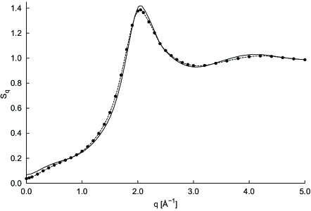
Fig. 1.: Structure factor of liquid ⁴He at the temperature $T=1.0$ K

Now, let us rewrite Eq. (3) in the form

$$\frac{1}{\alpha_{q_{1}}}=S^{\exp}(q_{1})\,-$$

$$-\,\frac{1}{\alpha^{2}_{q_{1}}}\biggl{[}\frac{1}{2N}\mathop{\sum_{\mathbf{k}_{2}\neq 0}\sum_{\mathbf{k}_{3}\neq 0}}\limits_{{\mathbf{q}}_{1}+{\mathbf{k}}_{2}+{\mathbf{k}}_{3}=0}\frac{\alpha_{k_{2}}-1}{\alpha_{k_{2}}}\frac{\alpha_{k_{3}}-1}{\alpha_{k_{3}}}\,+$$

$$+\,2a_{2}({\mathbf{q}_{1}})+\frac{2}{N}\mathop{\sum_{\mathbf{k}_{2}\neq 0}\sum_{\mathbf{k}_{3}\neq 0}}\limits_{{\mathbf{q}}_{1}+{\mathbf{k}}_{2}+{\mathbf{k}}_{3}=0}\frac{a_{3}({\mathbf{q}}_{1},{\mathbf{k}}_{2},{\mathbf{k}}_{3})}{\alpha_{k_{2}}\alpha_{k_{3}}}\,+$$

$$+\,\frac{1}{N}\!\!\sum_{\mathbf{k}_{2}\neq 0}\frac{a_{4}({\mathbf{q}}_{1},{\mathbf{k}}_{2})}{\alpha_{k_{2}}}+\frac{2}{N}\!\!\!\mathop{\sum_{\mathbf{k}_{2}\neq 0}\sum_{\mathbf{k}_{3}\neq 0}}\limits_{{\mathbf{q}}_{1}+{\mathbf{k}}_{2}+{\mathbf{k}}_{3}=0}\!\!\!\frac{a_{3}^{2}({\mathbf{q}}_{1},{\mathbf{k}}_{2},{\mathbf{k}}_{3})}{\alpha_{k_{2}}\alpha_{k_{3}}}\!\biggr{]}\!.$$ (4)

This is an iterative equation for $\alpha_{q}$.  In the zero-order approximation, we have $\alpha_{q}=1/S^{\exp}(q)$.  Substituting this $\alpha_{q}$-value into the right-hand side of equality (4), we obtain the $\alpha_{q}$-value in the first approximation, and so forth.  However, this iteration process does not converge, which is most likely connected with an insufficient number of terms in the series expansion for the structure factor (3).  Therefore, the consideration will be confined only to the zero-order approximation for $\alpha_{q}$.

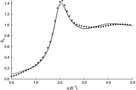
Fig. 2.: The same as in Fig. 1, but at $T=1.38$ K

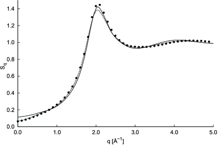
Fig. 3.: The same as in Fig. 1, but at $T=1.67$ K

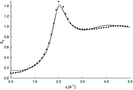
Fig. 4.: The same as in Fig. 1, but at $T=2.2$ K

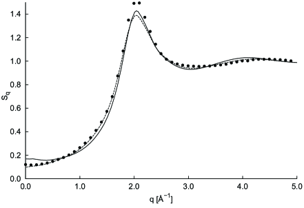
Fig. 5.: The same as in Fig. 1, but at $T=2.5$ K

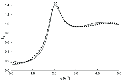
Fig. 6.: The same as in Fig. 1, but at $T=3.0$ K

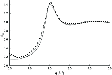
Fig. 7.: The same as in Fig. 1, but at $T=3.5$ K

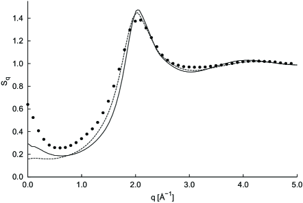
Fig. 8.: The same as in Fig. 1, but at $T=4.24$ K

The results of numerical calculations for temperatures of 1.0, 1.38, 1.67, 2.2, 2.5, 3.0, 3.5, and 4.24 K are exhibited in Figs. 1 to 8, respectively. Experimental data for the structure factor at those temperatures were taken from works [12,​ 13].  In the presented figures, the solid curves correspond to the structure factor calculated with regard for the direct three- and four-particle correlations, the dashed curves to the pair correlation approximation, and the circles to the experimental structure factor values.

7 Conclusions

In this work, expressions for the two-, three-, and four-particle structure factors in a wide temperature interval were found in the approximation “one sum over the wave vector” with regard for the direct three- and four-particle correlations.  In the low-temperature limit, the expression obtained for the two-particle structure factor transforms into the well-known one [21].  The same is valid for the high-temperature limit.

The derived expressions are rather cumbersome. They were analyzed, by using numerical methods, and graphic representations of the pair structure factor at various temperatures of liquid ⁴He were plotted.  The calculation of the internal energy and the determination of the temperature dependence of the first-sound velocity in the many-boson system will be a subject of our next papers.

APPENDIX 1

$$P(\rho|\rho^{\prime})=\exp\biggl{[}\frac{c_{0}}{N}+\sum_{\mathbf{q}_{1}\neq 0}\sum_{i_{1}=0}^{1}\sum_{j_{1}=0}^{1}c_{2}\left(1^{j1},-1^{i_{1}}\right)\times$$

$$\times\left(\rho_{\mathbf{q}_{1}}^{j_{1}}\rho_{-\mathbf{q}_{1}}^{i_{1}}+\rho_{\mathbf{q}_{1}}^{1-j_{1}}\rho_{-\mathbf{q}_{1}}^{1-i_{1}}\right)+$$

$$+\,\frac{1}{\sqrt{N}}\mathop{\sum_{\mathbf{q}_{1}\neq 0}\sum_{\mathbf{q}_{2}\neq 0}\sum_{\mathbf{q}_{3}\neq 0}}\limits_{\mathbf{q}_{1}+\mathbf{q}_{2}+\mathbf{q}_{3}\neq 0}\sum_{i_{1},i_{2},i_{3}=0}^{1}c_{3}(1^{i_{1}},2^{i_{2}},3^{i_{3}})\,\times$$

$$\times\left(\rho_{\mathbf{q}_{1}}^{i_{1}}\rho_{\mathbf{q}_{2}}^{i_{2}}\rho_{\mathbf{q}_{3}}^{i_{3}}+\rho_{\mathbf{q}_{1}}^{1-i_{1}}\rho_{\mathbf{q}_{2}}^{1-i_{2}}\rho_{\mathbf{q}_{3}}^{1-i_{3}}\!\right)+$$

$$+\,\frac{1}{N}\sum_{\mathbf{q}_{1}\neq 0}\sum_{\mathbf{q}_{2}\neq 0}\sum_{i_{1},i_{2}=0}^{1}\sum_{j_{1},j_{2}=0}^{1}c_{4}(1^{j_{1}},-1^{i_{1}},2^{j_{2}},-2^{i_{2}})\,\times$$

$$\times\,\left(\rho_{\mathbf{q}_{1}}^{j_{1}}\rho_{-\mathbf{q}_{1}}^{i_{1}}\rho_{\mathbf{q}_{2}}^{j_{2}}\rho_{-\mathbf{q}_{2}}^{i_{2}}+\rho_{\mathbf{q}_{1}}^{1-j_{1}}\rho_{-\mathbf{q}_{1}}^{1-i_{1}}\rho_{\mathbf{q}_{2}}^{1-j_{2}}\rho_{-\mathbf{q}_{2}}^{1-i_{2}}\!\right)\!\biggr{]}\!.$$

The superscripts $i_{1}$, $i_{2}$, $i_{3}$, $j_{1},$ and $j_{2}$ at the quantities $\rho_{\mathbf{q}}$ can acquire values of 0 or 1, namely, 0 means the absence of the prime, and 1 its presence.  The notation $c_{2}\left(1^{j1},-1^{i_{1}}\right)$ stands for $c_{2}\left(\rho_{q_{1}}^{j_{1}},\rho_{-q_{1}}^{i_{1}}\right)$, $c_{3}(1^{i_{1}},2^{i_{2}},3^{i_{3}})$ for $c_{3}(\rho_{q_{1}}^{i_{1}},\rho_{q_{2}}^{i_{2}},\rho_{q_{3}}^{i_{3}})$, and $c_{4}(1^{j_{1}},-1^{i_{1}},2^{j_{2}},-2^{i_{2}})$ for $c_{4}(\rho_{q_{1}}^{j_{1}},\rho_{-q_{1}}^{i_{1}},\rho_{q_{2}}^{j_{2}},\rho_{-q_{2}}^{i_{2}})$.  Accordingly,

$$c_{2}\left(1^{j1},-1^{i_{1}}\right)=\overline{c}_{2}\left(1^{j1},-1^{i_{1}}\right)-\overline{c}^{0}_{2}\left(1^{j1},-1^{i_{1}}\right)\!,$$

$$c_{3}(1^{i_{1}},2^{i_{2}},3^{i_{3}})=\overline{c}_{3}(1^{i_{1}},2^{i_{2}},3^{i_{3}})-\overline{c}^{0}_{3}(1^{i_{1}},2^{i_{2}},3^{i_{3}}),$$

$$c_{4}(1^{j_{1}},-1^{i_{1}},2^{j_{2}},-2^{i_{2}})=\overline{c}_{4}(1^{j_{1}},-1^{i_{1}},2^{j_{2}},-2^{i_{2}})\,-$$

$$-\,\overline{c}^{0}_{4}(1^{j_{1}},-1^{i_{1}},2^{j_{2}},-2^{i_{2}}).$$

Here, the quantities $\overline{c}_{0}^{0}$, $\overline{c}_{2}^{0}$, $\overline{c}_{3}^{0}$, and $\overline{c}_{4}^{0}$ mean $\overline{c}_{0}$, $\overline{c}_{2}$, $\overline{c}_{3}$, and $\overline{c}_{4}$, respectively, in which $\alpha_{q_{1}}=\alpha_{q_{2}}=\alpha_{q_{3}}=1$.  The quantity $\overline{c}_{4}(1^{j_{1}},-1^{i_{1}},2^{j_{2}},-2^{i_{2}})$ consists of two terms,

$$\overline{c}_{4}(1^{j_{1}},-1^{i_{1}},2^{j_{2}},-2^{i_{2}})=\overline{c}_{4}^{(1)}(1^{j_{1}},-1^{i_{1}},2^{j_{2}},-2^{i_{2}})\,+$$

$$+\,\overline{c}_{4}^{(2)}(1^{j_{1}},-1^{i_{1}},2^{j_{2}},-2^{i_{2}}),$$

where

$$\overline{c}_{4}^{(1)}(1^{j_{1}},-1^{i_{1}},2^{j_{2}},-2^{i_{2}})=$$

$$=-\frac{1}{64}\frac{\hbar^{2}}{2m}\frac{(-1)^{i_{1}+i_{2}+j_{1}+j_{2}}(q_{1}^{2}+q_{2}^{2})}{\operatorname{sh}^{2}(\beta E_{q_{1}})\operatorname{sh}^{2}(\beta E_{q_{2}})}\,\times$$

$$\times\!\sum_{\pm_{1}}\!\sum_{\pm_{2}}\!\sum_{\pm_{3}}\!\pm_{1}\!\pm_{2}\!\pm_{3}\!\frac{\operatorname{sh}\!\left[\frac{\beta}{2}(E_{q_{1}}\!\pm_{1}\!E_{q_{1}}\!\pm_{2}\!E_{q_{2}}\!\pm_{3}\!E_{q_{2}})\right]}{E_{q_{1}}\pm_{1}E_{q_{1}}\pm_{2}E_{q_{2}}\pm_{3}E_{q_{2}}}\,\times$$

$$\times\,\operatorname{ch}\biggl{[}\frac{\beta}{2}\biggl{(}\!(-1)^{i_{1}}E_{q_{1}}\pm_{1}(-1)^{j_{1}}E_{q_{1}}\pm_{2}$$

$$\pm_{2}(-1)^{i_{2}}E_{q_{2}}\pm_{3}(-1)^{j_{2}}E_{q_{2}}\!\biggr{)}\!\biggr{]}\!.$$

$$\overline{c}_{4}^{(2)}(1^{j_{1}},-1^{i_{1}},2^{j_{2}},-2^{i_{2}})=\frac{(-1)^{i_{1}+i_{2}+j_{1}+j_{2}}}{128\alpha_{q_{3}}}\left(\!\frac{\hbar^{2}}{2m}\!\right)^{\!\!2}\!\!\times$$

$$\times\,\frac{Q(\tilde{\alpha}_{q_{1}},\tilde{\alpha}_{q_{2}},\alpha_{q_{3}})}{\operatorname{sh}^{2}(\beta E_{q_{1}}\!)\operatorname{sh}^{2}(\beta E_{q_{2}}\!)\operatorname{sh}(\beta E_{q_{3}}\!)}\operatorname{sh}\!\left[\frac{\beta}{2}(\tilde{E}_{q_{1}}\!+\!\tilde{E}_{q_{2}}\!+\!E_{q_{3}})\right]\times$$

$$\times\biggl{\{}\!\frac{\beta}{\tilde{E}}\operatorname{sh}\left[\frac{\beta}{2}\left(\!(-1)^{i_{1}}\tilde{E}_{q_{1}}+(-1)^{i_{2}}\tilde{E}_{q_{2}}-E_{q_{3}}\!\right)\!\right]\times$$

$$\times\,Q(\tilde{\alpha}_{q_{1}},\tilde{\alpha}_{q_{2}},\alpha_{q_{3}})-\frac{2\operatorname{sh}\left[\frac{\beta}{2}\tilde{E}\right]}{\tilde{E}^{2}}Q(\tilde{\alpha}_{q_{1}},\tilde{\alpha}_{q_{2}},\alpha_{q_{3}})\,\times$$

$$\times\,\operatorname{ch}\left[\beta\left(\!(i_{1}-1)\tilde{E}_{q_{1}}+(i_{2}-1)\tilde{E}_{q_{2}}\!\right)\!\right]-$$

$$-\frac{2\operatorname{sh}\left[\frac{\beta}{2}\tilde{E}_{q_{2}}\right]}{\tilde{E}\tilde{E}_{q_{2}}}Q(\tilde{\alpha}_{q_{1}},-\tilde{\alpha}_{q_{2}},\alpha_{q_{3}})\,\times$$

$$\times\,\operatorname{ch}\left[\frac{\beta}{2}\left(\!(-1)^{i_{1}}\tilde{E}_{q_{1}}+2(i_{2}-1)\tilde{E}_{q_{2}}-E_{q_{3}}\!\right)\!\right]+$$

$$+\frac{2\operatorname{sh}\left[\frac{\beta}{2}(\tilde{E}_{q_{1}}+E_{q_{3}})\right]}{\tilde{E}(\tilde{E}_{q_{1}}+E_{q_{3}})}Q(\tilde{\alpha}_{q_{1}},-\tilde{\alpha}_{q_{2}},\alpha_{q_{3}})\,\times$$

$$\times\operatorname{ch}\left[\frac{\beta}{2}\left(\!2(i_{1}-1)\tilde{E}_{q_{1}}+(-1)^{i_{2}}\tilde{E}_{q_{2}}\!\right)\!\right]-$$

$$-\frac{2\operatorname{sh}\left[\frac{\beta}{2}\tilde{E}_{q_{1}}\right]}{\tilde{E}\tilde{E}_{q_{1}}}Q(-\tilde{\alpha}_{q_{1}},\tilde{\alpha}_{q_{2}},\alpha_{q_{3}})\times$$

$$\times\operatorname{ch}\left[\frac{\beta}{2}\left(\!(-1)^{i_{2}}\tilde{E}_{q_{2}}+2(i_{1}-1)\tilde{E}_{q_{1}}-E_{q_{3}}\!\right)\!\right]+$$

$$+\frac{2\operatorname{sh}\left[\frac{\beta}{2}(\tilde{E}_{q_{2}}+E_{q_{3}})\right]}{\tilde{E}(\tilde{E}_{q_{2}}+E_{q_{3}})}Q(-\tilde{\alpha}_{q_{1}},\tilde{\alpha}_{q_{2}},\alpha_{q_{3}})\times$$

$$\times\operatorname{ch}\left[\frac{\beta}{2}\left(\!2(i_{2}-1)\tilde{E}_{q_{2}}+(-1)^{i_{1}}\tilde{E}_{q_{1}}\!\right)\!\right]-$$

$$-\frac{2\operatorname{sh}\left[\frac{\beta}{2}E_{q_{3}}\right]}{\tilde{E}E_{q_{3}}}Q(-\tilde{\alpha}_{q_{1}},-\tilde{\alpha}_{q_{2}},\alpha_{q_{3}})\times$$

$$\times\operatorname{ch}\left[\frac{\beta}{2}\left(\!(-1)^{i_{2}}\tilde{E}_{q_{2}}+(-1)^{i_{1}}\tilde{E}_{q_{1}}\!\right)\!\right]+$$

$$+\frac{2\operatorname{sh}\left[\frac{\beta}{2}(\tilde{E}_{q_{1}}+E_{q_{2}})\right]}{\tilde{E}(\tilde{E}_{q_{1}}+E_{q_{2}})}Q(-\tilde{\alpha}_{q_{1}},-\tilde{\alpha}_{q_{2}},\alpha_{q_{3}})\times$$

$$\times\operatorname{ch}\left[\frac{\beta}{2}\left(\!2(i_{2}-1)\tilde{E}_{q_{2}}+2(i_{1}-1)\tilde{E}_{q_{1}}-E_{q_{3}}\!\right)\!\right]\!\biggr{\}}\!.$$

The coefficients $\overline{c}_{2}(1^{j_{1}},-1^{i_{1}})$ and $\overline{c}_{0}$ can be expressed in terms of $\overline{c}_{4}^{(1)}(1^{j_{1}},-1^{i_{1}},2^{j_{2}},-2^{i_{2}})$ and $\overline{c}_{4}^{(2)}(1^{j_{1}},-1^{i_{1}},2^{j_{2}},-2^{i_{2}})$ as follows:

$$\overline{c}_{2}(1^{j_{1}},-1^{i_{1}})=2\alpha_{q_{2}}\operatorname{sh}\left[\beta E_{q_{2}}\right]\times$$

$$\times\left(\!2\overline{c}_{4}^{(1)}(1^{j_{1}},-1^{i_{1}},2,-2^{\prime})+\overline{c}_{4}^{(2)}(1^{j_{1}},-1^{i_{1}},2,-2^{\prime})\!\right)\!,$$

$$\overline{c}_{0}=4\alpha_{q_{1}}\alpha_{q_{2}}\operatorname{sh}\left[\beta E_{q_{1}}\right]\operatorname{sh}\left[\beta E_{q_{2}}\right]\times$$

$$\times\left(\!2\overline{c}_{4}^{(1)}(1,-1^{\prime},2,-2^{\prime})+\frac{\overline{c}_{4}^{(2)}(1,-1^{\prime},2,-2^{\prime})}{3}\!\right)\!\!.$$

The quantity $\overline{c}_{3}(1^{i_{1}},2^{i_{2}},3^{i_{3}})$ looks like

$$\overline{c}_{3}(1^{i_{1}},2^{i_{2}},3^{i_{3}})\!=\!-\frac{1}{16}\frac{\hbar^{2}}{2m}\frac{(-1)^{i_{1}+i_{2}}(\bf{q}_{1}\bf{q}_{2})}{\operatorname{sh}[\beta E_{q_{1}}]\operatorname{sh}[\beta E_{q_{2}}]\operatorname{sh}[\beta E_{q_{3}}]}\,\times$$

$$\times\sum_{\pm_{1}}\sum_{\pm_{2}}\left(\alpha_{q_{1}}\alpha_{q_{2}}\pm_{1}\pm_{2}1\right)\frac{\operatorname{sh}\left[\frac{\beta}{2}\left(\tilde{E}_{q_{1}}+\tilde{E}_{q_{2}}+E_{q_{3}}\right)\right]}{\tilde{E}_{q_{1}}+\tilde{E}_{q_{2}}+E_{q_{3}}}\,\times$$

$$\times\,\operatorname{sh}\left[\frac{\beta}{2}\left(\!(-1)^{i_{1}}\tilde{E}_{q_{1}}+(-1)^{i_{2}}\tilde{E}_{q_{2}}+(-1)^{i_{3}}E_{q_{3}}\!\right)\!\right]\!.$$

In the expressions written above, the following notations were introduced:

$$\tilde{E}_{q_{1}}=\pm_{1}E_{q_{1}};\quad\tilde{E}_{q_{2}}=\pm_{2}E_{q_{1}};$$

$$\tilde{\alpha}_{q_{1}}=\pm_{1}\alpha_{q_{1}};\quad\tilde{\alpha}_{q_{2}}=\pm_{1}\alpha_{q_{2}};$$

$$\tilde{E}=\pm_{1}E_{q_{1}}\pm_{2}E_{q_{2}}+E_{q_{3}};$$

$$Q(\tilde{\alpha}_{q_{1}},\tilde{\alpha}_{q_{2}},\alpha_{q_{3}})=(\pm_{1}\pm_{2}\alpha_{q_{1}}\alpha_{q_{2}}+1)({\bf q}_{1}{\bf q}_{2})\,+$$

$$+\,(\pm_{1}\alpha_{q_{1}}\alpha_{q_{3}}+1)({\bf q}_{1}{\bf q}_{3})+(\pm_{2}\alpha_{q_{2}}\alpha_{q_{3}}+1)({\bf q}_{2}{\bf q}_{3}).$$

APPENDIX 2

$$C_{2}({\mathbf{q}_{1}})=\overline{C}_{2}({\mathbf{q}_{1}})-\overline{C}_{2}^{0}({\mathbf{q}_{1}}),$$

$$C_{3}({\mathbf{q}}_{1},{\mathbf{q}}_{2},{\mathbf{q}}_{3})=\overline{C}_{3}({\mathbf{q}}_{1},{\mathbf{q}}_{2},{\mathbf{q}}_{3})-\overline{C}_{3}^{0}({\mathbf{q}}_{1},{\mathbf{q}}_{2},{\mathbf{q}}_{3}),$$

$$C_{4}({\mathbf{q}}_{1},{\mathbf{q}}_{2})=\overline{C}_{4}({\mathbf{q}}_{1},{\mathbf{q}}_{2})-\overline{C}_{4}^{0}({\mathbf{q}}_{1},{\mathbf{q}}_{2}),$$

where

$$\overline{C}_{2}({\mathbf{q}_{1}})=\frac{1}{2}\!\!\!\sum_{i_{1}=0}^{1}\sum_{j_{1}=0}^{1}\!\!\overline{c}_{2}(1^{j1},-1^{i_{1}});$$

$$\overline{C}_{3}({\mathbf{q}}_{1},{\mathbf{q}}_{2},{\mathbf{q}}_{3})\!\!=\frac{1}{2}\!\!\sum_{i_{1},i_{2},i_{3}=0}^{1}\!\!\overline{c}_{3}(1^{i_{1}},2^{i_{2}},3^{i_{3}});$$

$$\overline{C}_{4}({\mathbf{q}}_{1},{\mathbf{q}}_{2})\!\!=\frac{1}{2}\!\!\sum_{i_{1},i_{2}=0}^{1}\sum_{j_{1},j_{2}=0}^{1}\!\!\!\overline{c}_{4}(1^{j_{1}},-1^{i_{1}},2^{j_{2}},-2^{i_{2}}).$$

The notations $\overline{C}_{2}^{0}({\mathbf{q}_{1}})$, $\overline{C}_{3}^{0}({\mathbf{q}}_{1},{\mathbf{q}}_{2},{\mathbf{q}}_{3})$, and $\overline{C}_{4}^{0}({\mathbf{q}}_{1},{\mathbf{q}}_{2})$ mean the quantities $\overline{C}_{2}({\mathbf{q}_{1}})$, $\overline{C}_{3}({\mathbf{q}}_{1},{\mathbf{q}}_{2},{\mathbf{q}}_{3})$, and $\overline{C}_{4}({\mathbf{q}}_{1},{\mathbf{q}}_{2})$, respectively, in which the Bogolyubov factor is equal to unity: $\alpha_{q_{1}}=\alpha_{q_{2}}=\alpha_{q_{3}}=1$.  The quantities $\overline{C}_{2}({\mathbf{q}_{1}})$, $\overline{C}_{3}({\mathbf{q}}_{1},{\mathbf{q}}_{2},{\mathbf{q}}_{3})$, and $\overline{C}_{4}({\mathbf{q}}_{1},{\mathbf{q}}_{2})$ themselves look like

$$\overline{C}_{2}({\bf q_{1}})=-\frac{1}{4}\sum_{{\bf q_{2}}\neq 0}\frac{\hbar^{2}}{2m}\frac{q_{1}^{2}+q_{2}^{2}}{\alpha_{q_{2}}\operatorname{ch}^{2}\left[\frac{\beta}{2}E_{q_{1}}\right]\operatorname{sh}[\beta E_{q_{2}}]}\,\times$$

$$\times\biggl{\{}\!\frac{\beta}{4}\operatorname{ch}[\beta E_{q_{2}}]-\frac{\operatorname{sh}[\beta E_{q_{2}}]}{4E_{q_{2}}}+\frac{\operatorname{sh}[\beta E_{q_{1}}]\operatorname{ch}[\beta E_{q_{2}}]}{4E_{q_{1}}}\,-$$

$$-\,\frac{\operatorname{sh}[\beta(E_{q_{1}}+E_{q_{2}})]}{8(E_{q_{1}}+E_{q_{2}})}-\frac{\operatorname{sh}[\beta(E_{q_{1}}-E_{q_{2}})]}{8(E_{q_{1}}-E_{q_{2}})}\biggr{\}}+\frac{1}{16}\left(\!\frac{\hbar^{2}}{2m}\!\right)^{\!\!2}\!\!\times$$

$$\times\!\!\!\mathop{\sum_{\mathbf{q}_{2}\neq 0}\sum_{\mathbf{q}_{3}\neq 0}}\limits_{\mathbf{q}_{1}+\mathbf{q}_{2}+\mathbf{q}_{3}=0}\frac{Q(\tilde{\alpha}_{q_{1}},\tilde{\alpha}_{q_{2}},\alpha_{q_{3}})\operatorname{ch}\left[\frac{\beta}{2}(\tilde{E}_{q_{2}}+E_{q_{3}})\right]}{\alpha_{q_{2}}\alpha_{q_{3}}\tilde{E}\operatorname{ch}^{2}\left[\frac{\beta}{2}E_{q_{1}}\right]\operatorname{sh}\left[\beta E_{q_{2}}\right]\operatorname{sh}\left[\beta E_{q_{3}}\right]}\times$$

$$\times\Bigg{\{}\!\frac{\beta}{4}\operatorname{sh}\left[\frac{\beta}{2}(\tilde{E}_{q_{2}}+E_{q_{3}})\right]Q(\tilde{\alpha}_{q_{1}},\tilde{\alpha}_{q_{2}},\alpha_{q_{3}})\,+$$

$$+\,\frac{1}{2}\operatorname{sh}\left[\frac{\beta}{2}\tilde{E}\right]\operatorname{sh}\left[\frac{\beta}{2}\tilde{E}_{q_{1}}\right]\times$$

$$\times\Bigg{(}\!\frac{Q(-\tilde{\alpha}_{q_{1}},\tilde{\alpha}_{q_{2}},\alpha_{q_{3}})}{\tilde{E}}+\frac{Q(\tilde{\alpha}_{q_{1}},\tilde{\alpha}_{q_{2}},\alpha_{q_{3}})}{\tilde{E}_{q_{1}}}\!\Bigg{)}-$$

$$-\,\frac{1}{2}\operatorname{sh}\left[\frac{\beta}{2}(\tilde{E}_{q_{1}}+\tilde{E}_{q_{2}})\right]\operatorname{sh}\left[\frac{\beta}{2}(\tilde{E}_{q_{1}}+E_{q_{3}})\right]\times$$

$$\times\Bigg{(}\!\frac{Q(-\tilde{\alpha}_{q_{1}},-\tilde{\alpha}_{q_{2}},\alpha_{q_{3}})}{\tilde{E}_{q_{1}}+\tilde{E}_{q_{2}}}+\frac{Q(\tilde{\alpha}_{q_{1}},\tilde{\alpha}_{q_{2}},\alpha_{q_{3}})}{\tilde{E}_{q_{1}}+E_{q_{3}}}\!\Bigg{)}-$$

$$-\,\frac{1}{2}\operatorname{sh}\left[\frac{\beta}{2}\tilde{E}_{q_{2}}\right]\operatorname{sh}\left[\frac{\beta}{2}E_{q_{3}}\right]\times$$

$$\times\Bigg{(}\!\frac{Q(\tilde{\alpha}_{q_{1}},-\tilde{\alpha}_{q_{2}},\alpha_{q_{3}})}{\tilde{E}_{q_{2}}}+\frac{Q(-\tilde{\alpha}_{q_{1}},-\tilde{\alpha}_{q_{2}},\alpha_{q_{3}})}{E_{q_{3}}}\!\Bigg{)}\!\!\Bigg{\}}\!.$$

$$\overline{C}_{3}({\bf q_{1}},{\bf q_{2}},{\bf q_{3}})=-\frac{1}{48}\frac{\hbar^{2}}{2m}\frac{\operatorname{sh}\left[\frac{\beta}{2}\tilde{E}\right]}{\tilde{E}\prod\limits_{j=1}^{3}\operatorname{ch}\left[\frac{\beta}{2}E_{q_{j}}\right]}\,\times$$

$$\times\,Q(\tilde{\alpha}_{q_{1}},\tilde{\alpha}_{q_{2}},\alpha_{q_{3}}).$$ (5)

$$\overline{C}_{4}({\bf q_{1}},{\bf q_{2}})=-\frac{1}{16}\sum_{{\bf q_{1}}\neq 0}\sum_{{\bf q_{2}}\neq 0}\frac{\hbar^{2}}{2m}\frac{(q_{1}^{2}+q_{2}^{2})}{\operatorname{ch}^{2}\left[\frac{\beta}{2}E_{q_{1}}\right]}\,\times$$

$$\times\,\frac{1}{\operatorname{ch}^{2}\left[\frac{\beta}{2}E_{q_{2}}\right]}\Bigg{\{}\!\frac{\beta}{4}+\frac{\operatorname{sh}[\beta E_{q_{2}}]}{4E_{q_{2}}}+\frac{\operatorname{sh}[\beta E_{q_{1}}]\operatorname{ch}[\beta E_{q_{2}}]}{4E_{q_{1}}}\,+$$

$$+\,\frac{\operatorname{sh}[\beta(E_{q_{1}}+E_{q_{2}})]}{8(E_{q_{1}}+E_{q_{2}})}\!+\!\frac{\operatorname{sh}[\beta(E_{q_{1}}-E_{q_{2}})]}{8(E_{q_{1}}-E_{q_{2}})}\biggr{\}}+\frac{1}{64}\left(\frac{\hbar^{2}}{2m}\right)^{\!\!2}\!\times$$

$$\times\mathop{\sum_{\mathbf{q}_{3}\neq 0}}\limits_{\mathbf{q}_{1}+\mathbf{q}_{2}+\mathbf{q}_{3}=0}\!\!\!\frac{Q(\tilde{\alpha}_{q_{1}},\tilde{\alpha}_{q_{2}},\alpha_{q_{3}})}{\alpha_{q_{3}}\tilde{E}\operatorname{ch}^{2}\left[\frac{\beta}{2}E_{q_{1}}\right]\operatorname{ch}^{2}\left[\frac{\beta}{2}E_{q_{2}}\right]\operatorname{ch}\left[\frac{\beta}{2}E_{q_{3}}\right]}\times$$

$$\times\Bigg{\{}\!\!\Bigg{(}\!\frac{\beta}{4}\!\operatorname{ch}\left[\frac{\beta}{2}E_{q_{3}}\right]\!-\!\frac{\operatorname{sh}\left[\frac{\beta}{2}\tilde{E}\right]}{2\tilde{E}}\operatorname{ch}\left[\frac{\beta}{2}(\tilde{E}_{q_{1}}\!+\!\tilde{E}_{q_{2}})\right]\!\!\Bigg{)}\times$$

$$\times\,Q(\!\tilde{\alpha}_{q_{1}}\!,\tilde{\alpha}_{q_{2}}\!,\alpha_{q_{3}}\!)\!+\!\Bigg{(}\!\frac{\operatorname{sh}\!\left[\frac{\beta}{2}\tilde{E}_{q_{2}}\right]}{2\tilde{E}_{q_{2}}}\operatorname{ch}\!\left[\frac{\beta}{2}(\tilde{E}_{q_{2}}\!+\!E_{q_{3}})\right]-$$

$$-\,\frac{\operatorname{sh}\!\left[\frac{\beta}{2}(\tilde{E}_{q_{1}}\!+\!E_{q_{3}})\right]}{2(\tilde{E}_{q_{1}}+E_{q_{3}})}\operatorname{ch}\!\left[\frac{\beta}{2}\tilde{E}_{q_{2}}\right]\!\!\Bigg{)}\!Q(\tilde{\alpha}_{q_{1}},-\tilde{\alpha}_{q_{2}},\alpha_{q_{3}})\,+$$

$$+\Bigg{(}\!\frac{\operatorname{sh}\left[\frac{\beta}{2}\tilde{E}_{q_{1}}\right]}{2\tilde{E}_{q_{1}}}\operatorname{ch}\left[\frac{\beta}{2}(\tilde{E}_{q_{1}}+E_{q_{3}})\right]-$$

$$-\frac{\operatorname{sh}\!\left[\frac{\beta}{2}(\tilde{E}_{q_{2}}\!+\!E_{q_{3}})\right]}{2(\tilde{E}_{q_{2}}+E_{q_{3}})}\operatorname{ch}\!\left[\frac{\beta}{2}\tilde{E}_{q_{1}}\right]\!\!\Bigg{)}\!Q(-\tilde{\alpha}_{q_{1}},\tilde{\alpha}_{q_{2}},\alpha_{q_{3}})\,+$$

$$+\Bigg{(}\!-\frac{\operatorname{sh}\!\left[\frac{\beta}{2}E_{q_{3}}\right]}{2E_{q_{3}}}\!+\!\frac{\operatorname{sh}\!\left[\frac{\beta}{2}(\tilde{E}_{q_{1}}\!+\!\tilde{E}_{q_{2}})\right]}{2(\tilde{E}_{q_{1}}+\tilde{E}_{q_{2}})}\operatorname{ch}\!\left[\frac{\beta}{2}\tilde{E}\right]\!\!\Bigg{)}\times$$

$$\times\,Q(-\tilde{\alpha}_{q_{1}},-\tilde{\alpha}_{q_{2}},\alpha_{q_{3}})\!\Bigg{\}}\!.$$

I.О. Вакарчук, О.I. Григорчак
СТРУКТУРНI ФУНКЦIЇ
БАГАТОБОЗОННОЇ СИСТЕМИ
IЗ ВРАХУВАННЯМ ПРЯМИХ ТРИ-
ТА ЧОТИРИЧАСТИНКОВИХ КОРЕЛЯЦIЙ
Р е з ю м е
На основi виразу для матрицi густини взаємодiючих бозе-частинок в координатному зображеннi iз врахуванням прямих три- i чотиричастинкових кореляцiй [I. О. Вакарчук, О. I. Григорчак, Журн. фiз. досл. 3, 3005 (2009)] були розрахованi дво-, три- i чотиричастинковi структурнi фактори рiдкого ⁴He в наближеннi ‘‘однiєї суми за хвильовим вектором’’ для широкого iнтервалу температур. В границi низьких температур отриманий вираз для двочастинкового структурного фактора переходить в уже вiдомий. В границi високих температур вирази для дво-, три- i чотиричастинкових структурних факторiв редукуються до структурних факторiв iдеального бозе-газу. Результати роботи можуть бути застосованi для розрахунку термодинамiчних функцiй рiдкого ⁴He i знаходження температурної залежностi швидкостi першого звуку в багатобозоннiй системi.

References

• [1] I.V. Bogoyavlenskii, A.V. Puchkov, and A. Skomorokhov, Physica B 284–288, 25 (2000).
• [2] Fereydoon Family, Physica B + C 107, 699 (1981).
• [3] F. Zambelli, L. Pitaevskii, D.M. Stamper-Kurn, and S. Stringari, Phys. Rev. A 61, 063608 (2000).
• [4] E. Krotscheck and T. Lichtenegger, J. Low Temp. Phys. 178, 61 (2015).
• [5] R. Hobbiger, R. Holler, E. Krotscheck, and M. Panholzer, J. Low Temp. Phys. 169, 350 (2012).
• [6] V. Sorkin, E. Polturak, and J. Adler, J. Low Temp. Phys. 143, 141 (2006).
• [7] E. Krotscheck and C.J. Tymczak, Phys. Rev. B 45, 217 (1992).
• [8] K, Miyazaki and I.M. de Schepper, Phys. Rev. E 63 060201 (2001).
• [9] V.B. Bobrov, S.A. Trigger, and Yu.P. Vlasov, Phys. B: Cond. Matt. 203, 95 (1994).
• [10] J. Dawidowski, F. J. Bermejo, M. L. Ristig, B. Fȧk, C. Cabrillo, R. Fernández-Perea, K. Kinugawa, and J. Campo, Phys. Rev. B 69, 014207 (2004).
• [11] F. Hayot and C. Jayaprakash, Phys. Rev. E 57, 4867(R) (1998).
• [12] E.C. Svensson, V.F. Sears, A.D.B. Woods, and P. Martel, Phys. Rev. B 21, 3638 (1980).
• [13] H.N. Robkoff and R.B. Hallock, Phys. Rev. B 24, 159 (1981).
• [14] F. Caupin, J. Boronat, and K.H. Andersen, J. Low Temp. Phys. 152, 108 (2008).
• [15] J. Steinhauer, R. Ozeri, N. Katz, and N. Davidson, Phys. Rev. A 72, 023608 (2005).
• [16] Chia-Wei Woo and R.L. Coldwell, Phys. Rev. Lett. 29, 1062 (1972).
• [17] N.G. Almarza, E. Lomba, and D. Molina, Phys. Rev. E 70, 021203 (2004).
• [18] P. Ziń, M. Trippenbach, and M. Gajda, Phys. Rev. A 69, 023614 (2004).
• [19] I.A. Vakarchuk and I.R. Yukhnovskii, Theor. Math. Phys. 40, 626 (1979); 42, 73 (1980).
• [20] I.A. Vakarchuk, A.L. Gonopolskii, and I.R. Yukhnovskii, Theor. Math. Phys. 41, 896 (1979).
• [21] I.A. Vakarchuk, Theor. Math. Phys. 65, 1164 (1985); 82, 308 (1990).
• [22] I.A. Vakarchuk and P.A. Glushak, Theor. Math. Phys. 75, 399 (1988).
• [23] P.A. Glushak, Research of Equilibrium Properties of Superfluid Helium-4 at Low Temperatures, Ph.D. thesis (Lviv, 1992) (in Russian).
• [24] I.O. Vakarchuk, R.O. Prytula, and A.A. Rovenchak, J. Phys. Stud. 11, 259 (2007).
• [25] I.O. Vakarchuk and R.O. Prytula, J. Phys. Stud. 12, 4001 (2008); 13, 2003 (2009).
• [26] F.K. Achter and L. Meyer, Phys. Rev. 188, 291 (1969).
• [27] Physics of Simple Liquids, edited by H.N.V. Temperley, J.S. Rowlinson, and G.S. Rushbrooke (North-Holland, Amsterdam, 1968).
• [28] C.A. Croxton, Liquid State Physics: A Statistical Mechanical Introduction (Cambridge Univ. Press, Cambridge, 2009).
• [29] I.O. Vakarchuk and O.I. Hryhorchak, J. Phys. Stud. 3, 3005 (2009).
• [30] I.O. Vakarchuk and O.I. Hryhorchak, Visn. L’viv. Univ. Ser. Fiz. 46, 3 (2011).
• [31] I.O. Vakarchuk, V.V. Babin, and A.A. Rovenchak, J. Phys. Stud. 4, 16 (2000).
• [32] A.A. Rovenchak, Self-Consistent Calculation of Interatomic Potentials and Thermodynamic Functions of Helium-4 in Superfluid and Normal Phases, Ph.D. thesis (Lviv, 2003) (in Ukrainian).
• [33] I.O. Vakarchuk, O.I. Hryhorchak, V.S. Pastukhov, and R.O. Prytula, arXiv:1506.03317 (2015).
• [34] I.O. Vakarchuk, J. Phys. Stud. 8, 223 (2004).
• [35] I.O. Vakarchuk, Introduction to Many-Body Problem (Lviv National Univ., Lviv, 1999) (in Russian).
• [36] R.J. Donnelly and C.F. Barenghi, J. Phys. Chem. Ref. Data 27, 1217 (1998).
Received 01.04.15.
Translated from Ukrainian by O.I. Voitenko