Relativistic quantum dynamics of neutral particle in external electric fields: An approach on effects of spin

Abstract

The planar quantum dynamics of spin-1/2 neutral particle interacting with electrical fields is considered. A set of first order differential equations are obtained directly from the planar Dirac equation with nonminimum coupling. New solutions of this system, in particular, for the Aharonov-Casher effect, are found and discussed in detail. Pauli equation is also obtained by studying the motion of the particle when it describes a circular path of constant radius. We also analyze the planar dynamics in the full space, including the $r=0$ region. The self-adjoint extension method is used to obtain the energy levels and wave functions of the particle for two particular values for the self-adjoint extension parameter. The energy levels obtained are analogous to the Landau levels and explicitly depend on the spin projection parameter.

1 Introduction

Topological effects in quantum mechanics has been one of the most studied problems of planar dynamics in recent years. These phenomena present no classical counterparts and are associated with physical systems defined on a multiply connected space-time PRL.1995.74.2847 . Many of the recent interest in this matter is a consequence of the pioneering work by Aharonov and Bohm (AB) PR.1959.115.485 , where they proposed the first example of generation of topological phase acquired by an electron when it travels through a magnetic field-free region. This phenomenon, known as Aharonov-Bohm effect, has been the usual framework for studying properties of other physical systems which lead to similar effects. The first subsequent effect was the work by Aharonov-Casher (AC) PRL.1984.53.319 , where they predicted that the wave function of a neutral particle with a magnetic dipole moment acquires a topological phase when traveling in a closed path which encircles an infinitely long filament carrying an uniform charge density. Subsequently, several other AB-like effects were discovered over the last three decades (see Refs. PRL.1987.58.1593 ; PRL.1990.65.1697 ; PRA.1993.47.3424 ; PRL.1995.75.2071 ; PRL.1994.72.5 ; PRL.2000.85.1354 ).

An important question that we address here are the effects of spin on the dynamics of topological effects. The first work in this context was proposed by Hagen to study the scattering of relativistic spin-1/2 particles in an AB potential PRL.1990.64.503 . He showed that, by reformulating the problem with a source of finite radius which is then allowed to go to zero, it is established that the delta function alone that causes solutions that are singular at the origin. He also concluded that the modifications in the amplitude which arise from the inclusion of spin are seen to modify the cross section for the case of polarized beams. Hagen has also shown that there is an exact equivalence between the AB effect for spin-1/2 particles and the AC effect PRL.1990.64.2347 . This fact establishes the dynamics of the AC problem. However, a peculiarity that Hagen has not addressed clearly in their work is how to find the bound states energy levels. By modeling the problem by boundary conditions at the origin, an expression for the bound state energy for the AC problem was derived in Ref. EPJC.2013.73.2402 . The method used to find these energies was established in Refs. PRD.2012.85.041701 ; AoP.2013.339.510 , and it is based on the self-adjoint extension method of operators in quantum mechanics.

In the AC problem, the electric field is the one generated by an infinitely long, infinitesimally thin line of charge along the $z$-axis with a charge density $\lambda_{1}$ distributed uniformly about it, namely

$$\mathbf{E}_{1}=2\lambda_{1}\frac{\mathbf{\hat{\rho}}}{\rho},~{}~{}~{}\mathbf{\nabla}\cdot\mathbf{E}_{1}=2\lambda_{1}\frac{\delta(\rho)}{\rho},$$ (1)

As pointed out in Ref. PRL.1990.64.2347 , to ensure the exact equivalence between the AB and AC effects, we can not neglect the $\boldsymbol{\nabla}\cdot\mathbf{E}_{1}$ term. The physical implications of this term on the dynamics of the particle has been quite studied in recent years EPL.2013.101.51005 ; EPJC.2014.74.2708 ; JPA.2010.43.354008 ; JPG.2013.40.075007 .

Another configuration field of interest is

$$\mathbf{E}_{2}=\frac{\lambda_{2}\rho}{2}\mathbf{\hat{\rho}},~{}~{}~{}\mathbf{\nabla}\cdot\mathbf{E}_{2}=\lambda_{2},~{}\frac{\partial\mathbf{E}_{2}}{\partial t}=0,~{}~{}~{}\mathbf{\nabla}\times\mathbf{E}_{2}=0.$$ (2)

This special configuration was proposed by Ericsson and Sjöqvist to study an atomic analog of the Landau quantization based on the AC effect PRA.2001.65.013607 . They demonstrated that the existence of a certain field-dipole configuration in which an atomic analog of the standard Landau effect occurs opens up the possibility for an atomic realization of the quantum Hall effect using electric fields. This same configuration was used to study the Landau levels in the nonrelativistic dynamics of a neutral particle which possesses a permanent magnetic dipole moment interacting with an external electric field in the curved spacetime background with either the presence or the absence of a torsion field PRD.2009.79.024008 (see also Ref. PRA.2009.80.032106 ).

In this article, we analyze the planar motion of a neutral particle of spin-1/2 interacting with both electric fields of Eqs. (1) and (2), i.e.,

$$\mathbf{E}=\mathbf{E}_{1}+\mathbf{E}_{2}.$$ (3)

Although the field configuration (1) has been studied in different contexts in the literature, in our approach, we solve the first order Dirac equation and derive their solutions giving a focus to the effects due to the spin. This analysis, in particular to the electric field of Eq. (1), which is responsible for the AC problem, it is presented and discussed in detail here for the first time. We also address the second-order Dirac equation, which results in the Pauli equation. We make use of the self-adjoint extension method Book.1975.Reed.II and model the Hamiltonian by boundary conditions CMP.1991.139.103 . We also determine an expression for the energy levels of the particle and compare it with the known results in the literature.

This paper is organized as follows. In Sec. 2, we consider the Dirac equation with nonminimal coupling and construct the set of first order differential equations. In Sec. 3, we solve the first order differential equations and obtain the bound state solutions of the particle. The existence of these solutions means that the system admits isolated solutions. In Sec. 4, we derive the second-order equation (Pauli equation) and solve it by assuming that the particle describes a circular path of constant radius. In Sec. 5, we analyze the dynamics of the system with the inclusion of the $r=0$ region. We use the self-adjoint extension method to fix the physics of the problem in the $r=0$ region. Expressions for the wave functions and energies are obtained, without any arbitrary parameter which arises from the self-adjoint extension approach. In Sec. 6, the results of Sec. 5 are examined in the nonrelativistic limit. In Sec. 7, we present our conclusions.

2 Equation of motion

We start with the Dirac equation with nonminimal coupling ($\hbar=c=1$)

$$\left[i\gamma^{\mu}\partial_{\mu}-\frac{\mu}{2}\sigma^{\mu\nu}F_{\mu\nu}-M\right]\psi=0,$$ (4)

where $\mu$ is the magnetic dipole moment of the particle, $F_{\mu\nu}$ is the electromagnetic tensor whose components are given by

$$F_{0i} = E^{i}=-E_{i},$$ (5)

$$F_{ij} = -\varepsilon_{ijk}B^{k}=\varepsilon_{ijk}B_{k},$$ (6)

and

$$\left(\sigma^{0j},\sigma^{ij}\right)=\left(i\alpha^{j},-\epsilon_{ijk}\Sigma^{k}\right),$$ (7)

where $\Sigma^{k}$ is the spin vector, are the components of the operator

$$\sigma^{\mu\nu}=\frac{i}{2}\left[\gamma^{\mu},\gamma^{\nu}\right].$$ (8)

As the particle interacts only with electric fields, we consider only (5). In the above representation, Eq. (4) can be written as

$$\left[\beta\gamma^{i}p_{i}+\beta m-i\mu\beta\gamma^{i}E_{i}\right]\psi=\mathcal{E}\psi.$$ (9)

Following Ref. PRL.1990.64.503 , we write $\gamma^{i}$ as

$$\gamma^{i}=is\epsilon_{ij}\beta\gamma^{j},$$ (10)

so that Eq. (9) becomes

$$\left[\beta\gamma^{i}p_{i}+\beta m-\mu s\beta\gamma^{i}\check{E}_{i}\right]\psi=\mathcal{E}\psi,$$

where $\check{E}_{i}=\epsilon_{ij}E_{j}$, $\epsilon_{ij}=-\epsilon_{ji}$. Equation (9) can be written as

$$\left[\beta\boldsymbol{\gamma}\cdot\left(\mathbf{p}-\mu s\boldsymbol{\check{E}}\right)+\beta m\right]\Psi=\mathcal{E}\psi.$$ (11)

The $\gamma$ matrices are conveniently defined in terms of the Pauli matrices  as PRL.1990.64.503

$$\beta\gamma_{1}=\sigma_{1},\qquad\beta\gamma_{2}=s\sigma_{2},\qquad\beta=\sigma_{3},$$ (12)

where $s$ is twice the spin value, with $s=+1$ for spin “up” and $s=-1$ for spin “down”. Thus, Eq. (11) can be written as

$$\left[\sigma_{1}\left(p_{1}-\mu s\check{E}_{1}\right)+s\sigma_{2}\left(p_{2}-\mu s\check{E}_{2}\right)+\sigma_{3}M\right]\psi=\mathcal{E}\psi.$$ (13)

By noting that $\check{E}_{1}=E_{2}$ e $\check{E}_{2}=-E_{1}$, as usual, we write Eq. (13) in polar coordinates $(\rho,\varphi)$

$$\left[-i\frac{\partial}{\partial\rho}-is\frac{1}{\rho}\frac{\partial}{i\partial\varphi}-i\left(\frac{\eta_{1}}{\rho}+\eta_{2}\rho\right)\right]\psi_{2}$$

$$=\mathrm{e}^{+is\phi}\left(\mathcal{E}-M\right)\psi_{1},$$ (14)

$$\left[-i\frac{\partial}{\partial\rho}+is\frac{1}{\rho}\frac{\partial}{i\partial\varphi}+i\left(\frac{\eta_{1}}{\rho}+\eta_{2}\rho\right)\right]\psi_{1}$$

$$=\mathrm{e}^{-is\phi}\left(\mathcal{E}+M\right)\psi_{2},$$ (15)

where $\eta_{1}=2\mu\lambda_{1},~{}\eta_{2}=\mu\lambda_{2}/2$. Using the decomposition

$$\psi=\left(\begin{array}[]{c}\psi_{1}\\ \psi_{2}\end{array}\right)=\left[\begin{array}[]{c}\sum_{m}f_{m}(\rho)e^{im\phi}\\ \sum_{m}ig_{m}(\rho)e^{i(m+s)\phi}\end{array}\right],$$ (16)

where $m=0,\pm 1,\pm 2,\pm 3,\ldots$ is the angular momentum quantum number, Eqs. (14)-(15) provide two coupled first-order radial equations

$$\left[\frac{d}{d\rho}+\frac{sm+\eta_{1}+1}{\rho}+\eta_{2}\rho\right]g_{m}(\rho)=\left(\mathcal{E}-M\right)f_{m}(\rho),$$ (17)

$$\left[-\frac{d}{d\rho}+\frac{sm+\eta_{1}}{\rho}+\eta_{2}\rho\right]f_{m}(\rho)=\left(\mathcal{E}+M\right)g_{m}(\rho).$$ (18)

The factor $i$ on the lower spinor component in Eq. (16) was inserted to ensure that the radial part of the spinors is manifestly real. An isolated solution for the problem can be obtained considering the particle at rest, i.e., $\mathcal{E}=\pm M$. Such solution for the Dirac equation in $(1+1)$ dimensions was investigated in Ref. AoP.2013.338.278 (see also Refs. JPA.2007.40.263 ; PLA.2006.351.379 ).

3 Isolated solutions and the Aharonov-Casher problem

In order to obtain isolated solutions, let us look for bound state solutions subjected to the normalization condition

$$\int_{0}^{\infty}\left(|f_{m}(\rho)|^{2}+|g_{m}(\rho)|^{2}\right)\rho d\rho=1,$$ (19)

and consider the conditions $\mathcal{E}=\pm M$ stated above.

3.1 Case $\mathcal{E}=M$

In this case, Eqs. (17)-(18) are written as

$$\left[\frac{d}{d\rho}+\frac{sm+\eta_{1}+1}{\rho}+\eta_{2}\rho\right]g_{m}(\rho)=0,$$ (20)

$$\left[-\frac{d}{d\rho}+\frac{sm+\eta_{1}}{\rho}+\eta_{2}\rho\right]f_{m}(\rho)=2Mg_{m}(\rho).$$ (21)

The solutions to $g_{m}(\rho)$ and $f_{m}(\rho)$ are

$$g_{m}(\rho)=c_{2}\,\rho^{-\left(ms+\eta_{1}+{1}\right)}\,e^{-\frac{\eta_{2}}{2}\rho^{2}}{,}$$ (22)

$$f_{m}(\rho)=\rho^{ms+\eta_{1}}~{}e^{\frac{\eta_{2}}{2}\rho^{2}}$$

$$\times\left[c_{1}+c_{2}M\left(\eta_{2}\right)^{ms+\eta_{1}}~{}\Gamma\left(-sm-\eta_{1},\eta_{2}\rho^{2}\right)\right],$$ (23)

where $c_{1}$ and $c_{2}$ are constants, and $\Gamma\left(-sm-\eta_{1},\eta_{2}\rho^{2}\right)$ is the upper incomplete Gamma function, obtained through the relation Book.1972.Abramowitz

$$\Gamma(a,x)=\int_{x}^{\infty}t^{a-1}e^{-t}dt,\qquad\Re(a)>0.$$ (24)

As $\eta_{1,2}\gtrless 0$, then $g_{m}(\rho)$ converges as $\rho\rightarrow 0$. Moreover, since $\Gamma\left(-sm-\eta_{1},\eta_{2}\rho^{2}\right)$ always diverges, then $f_{m}(\rho)$ will only converge if $c_{2}=0$ e $\eta_{2}<0$. As a result, we have

$$\left[\begin{array}[]{c}f_{m}(\rho)\\ g_{m}(\rho)\end{array}\right]=c_{1}\left(\begin{array}[]{c}1\\ 0\end{array}\right)\rho^{\eta_{1}+ms}e^{\frac{\eta_{2}}{2}\rho^{2}},~{}\left\{\begin{tabular}[]{l} $s=\pm 1,$\\ $\eta_{1}\gtrless 0,$\\ $\eta_{2}<0,$\\ $c_{2}=0,$\end{tabular}\ \right..$$ (25)

3.2 Case $\mathcal{E}=-M$

In this case, Eqs. (17)-(18) become

$$\left[\frac{d}{d\rho}+\frac{sm+\eta_{1}+1}{\rho}+\eta_{2}\rho\right]g_{m}(\rho) =-2Mf_{m}(\rho),$$ (26)

$$\left[-\frac{d}{d\rho}+\frac{sm+\eta_{1}}{\rho}+\eta_{2}\rho\right]f_{m}(\rho) =0.$$ (27)

The solutions of these equation are

$$f_{m}\left(\rho\right)=c_{1}\rho^{ms+\eta_{1}}~{}e^{\frac{\eta_{2}}{2}\rho^{2}},$$ (28)

$$g_{m}(\rho)=e^{-\frac{1}{2}\eta_{2}\rho^{2}}\rho^{-\left(sm+\eta_{1}+1\right)}$$

$$\times\left[c_{2}+c_{1}M\left(-\eta_{2}\right){}^{-\left(sm+\eta_{1}+1\right)}~{}\Gamma\left[ms+\eta_{1}+1,-\eta_{2}\rho^{2}\right]\right].$$ (29)

As for the case $\mathcal{E}=M$, looking for solutions ( 28) and (29), we can see that the only square integrable solutions are

$$\left[\begin{array}[]{c}f_{m}(\rho)\\ g_{m}(\rho)\end{array}\right]=c_{2}\left(\begin{array}[]{c}0\\ 1\end{array}\right)e^{-\frac{1}{2}\eta_{2}\rho^{2}}\rho^{-\left(sm+\eta_{1}+1\right)},~{}\left\{\begin{tabular}[]{l} $s=\pm 1,$\\ $\eta_{1}\gtrless 0,$\\ $\eta_{2}>0,$\\ $c_{1}=0,$\end{tabular}\right..$$ (30)

In summary, note that the above results, Eqs. (25) and (30) are bound-state solutions of square-integrable because the function $e^{\frac{\pm\eta_{2}}{2}\rho^{2}}$ with $\eta_{2}\lessgtr 0$ predominates over the polynomials $\rho^{\eta_{1}+ms}$ and $\rho^{-(sm+\eta_{1}+1)}$ for $\mathcal{E}=M$ and $\mathcal{E}=-M$, respectively. We can conclude that the presence of the $\lambda_{2}$ is necessary for the existence of bound states.

4 The quadratic equation

The equation of second order derivative of Eq. (11) is found to be

$$\left[\mathbf{p}+s(\mathbf{\mu}\times\mathbf{E})\right]^{2}\psi+\mu\sigma_{3}(\mathbf{\nabla}\cdot\mathbf{E})\psi=\left(\mathcal{E}^{2}-{}M^{2}\right)\psi.$$ (31)

Using (3), Eq. (31) can be written more explicitly as

$$\Bigg{[}-\frac{\partial^{2}}{\partial\rho^{2}}-\frac{1}{\rho}\frac{\partial}{\partial\rho}-\frac{1}{\rho^{2}}\frac{\partial^{2}}{\partial\varphi^{2}}+\,2s\left(\frac{\eta_{1}}{\rho}+\eta_{2}\rho\right)\frac{1}{\rho}\frac{\partial}{i\partial\varphi}$$ (32)

$$+\left(\frac{\eta_{1}}{\rho}+\eta_{2}\rho\right)^{2}\Bigg{]}\psi+\sigma_{z}\left[\eta_{1}\frac{\delta\left(\rho\right)}{\rho}+2\eta_{2}\right]\psi$$

$$= \left(\mathcal{E}^{2}-{}M^{2}\right)\psi,$$

In this stage, it is worthwhile to mention that Eq. (32) is the correct quadratic form of the Dirac equation with nonminimal coupling, because the singular term from $\mathbf{\nabla}\cdot\mathbf{E}_{1}$ is considered.

Using the decomposition (16), the equation for $f_{m}(\rho)$ can be obtained

$$hf_{m}(\rho)=Ef_{m}(\rho),$$ (33)

with $E=\mathcal{E}^{2}-M^{2}-2\eta_{2}\left(\eta_{1}+ms+1\right)$, where

$$h=h_{0}+\eta_{1}\frac{\delta\left(\rho\right)}{\rho},$$ (34)

is the Hamiltonian system with the magnetic moment of the particle pointing the positive direction of z axis, and

$$h_{0}=-\frac{d^{2}}{d\rho^{2}}-\frac{1}{\rho}\frac{d}{d\rho}+\frac{\nu^{2}}{\rho^{2}}+\eta_{2}^{2}\rho^{2}.$$ (35)

is Hamiltonian without the $\delta$ function, and

$$\nu=m+s\eta_{1}.$$ (36)

The equation for $g_{m}(\rho)$ is obtained in an immediate way. It is given by

$$\bar{h}g_{m}(\rho)=\bar{E}g_{m}(\rho),$$ (37)

with $\bar{E}=\left(\mathcal{E}^{2}-M^{2}\right)-2\eta_{2}\left[s\left(m+s\right)+\eta_{1}-1\right]$, where

$$\bar{h}=\bar{h}_{0}-\eta_{1}\frac{\delta\left(\rho\right)}{\rho},$$ (38)

$$\bar{h}_{0}=-\frac{d^{2}}{d\rho^{2}}-\frac{1}{\rho}\frac{d}{d\rho}+\frac{\bar{\nu}^{2}}{\rho^{2}}+\eta_{2}^{2}\rho^{2},$$ (39)

and

$$\bar{\nu}=m+s+s\eta_{1}.$$ (40)

Equation (32) governs the system dynamics. In this dynamic, we must consider regular and irregular solutions, since irregular solutions are also physical solutions for the system under consideration. In other words, since we consider the effects of the spin of the particle and because of the field configuration (1), the Hamiltonian will contain a singular potential. We will return to this problem in Section 5.

4.1 Particle in a ring of constant radius

Before solving Eq. (32), an interesting case which can be considered here is when we assume the particle describing a circular motion of radius $\rho=a=const.$. In this case, from (32) we get

$$\left[\frac{1}{a}\frac{\partial}{i\partial\varphi}+s\left(\frac{\eta_{1}}{a}+\eta_{1}a\right)\right]^{2}\psi=\left(\mathcal{E}^{2}-{}M^{2}\right)\psi.$$ (41)

According to Eq. (16), the wave function for a particle executing a circular motion of constant radius can be written as

$$\psi=\left[\begin{array}[]{c}a_{m}\\ ib_{m}e^{is\phi}\end{array}\right]e^{im\phi}.$$ (42)

If $\psi$ is an eigenvector of $\sigma_{z}$ with eigenvalue $\varsigma=\pm 1$, the energy levels are given by

$$\mathcal{E}^{2}-{}M^{2} =\left[\frac{m}{a}+s\left(\frac{\eta_{1}}{a}+\eta_{2}a\right)\right]^{2},~{}~{}\left(\varsigma=+1\right)$$ (43)

$$\mathcal{E}^{2}-{}M^{2} =\left[\frac{m+s}{a}+s\left(\frac{\eta_{1}}{a}+\eta_{2}a\right)\right]^{2},~{}~{}\left(\varsigma=-1\right)$$ (44)

The profiles of the energy is shown in Fig. 1 for $\varsigma=1$ and some values of $m$. Figure 1 clearly shows that both particle and antiparticle energy levels are members of the spectrum. Note that for positive (negative)-energy we find that the lowest quantum number corresponds to the lowest (highest) energies, so that it is plausible to identify them with particle (antiparticle) energy levels. Also, it is noticeable that the Dirac energies are symmetrical about $\mathcal{E}=0$ and since the positive and negative energies never intercept one can see that there is no channel for spontaneous particle-antiparticle creation.

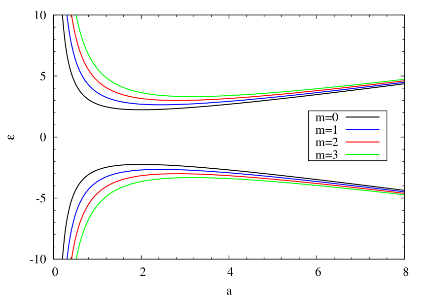
Figure 1: Plots of the energy as a function of radius for $\varsigma=1$ and different values of $m$.

If $\eta_{2}=0$, we obtain the energy levels of a neutral particle with magnetic moment $\mu$ in a circular path of constant radius,

$$\mathcal{E}^{2}-{}M^{2} = \frac{1}{a^{2}}\left(m+s\eta_{1}\right)^{2},$$ (45)

$$\mathcal{E}^{2}-{}M^{2} = \frac{1}{a^{2}}\left(m+s+s\eta_{1}\right)^{2}.$$ (46)

These energies correspond to spectrum for the usual Aharonov-Casher effect.

5 Self-adjoint extension analysis and the dynamic including the $r=0$ region

In this section, we solve Eqs. (33) and (37), including the term $\delta\left(\rho\right)/\rho$. In order to deal with this kind of point interaction potential, we consider the self-adjoint extension approach Book.2004.Albeverio ; JMP.1985.26.2520 . In quantum mechanics, observables correspond to self-adjoint operators. However, in some physical systems, we deal with differential operators for which the Hamiltonian is not necessarily symmetrical in some region of the space. In such cases, the Hamiltonian is not essentially self-adjoint and one attempts to find self-adjoint extensions of the Hamiltonian corresponding to different types of boundary conditions. Such self-adjoint extensions are based in boundary conditions at the origin and conditions at infinity crll.1987.380.87 ; JMP.1998.39.47 ; LMP.1998.43.43 . From the theory of symmetric operators, it is a well-known fact that the symmetric radial operator $h_{0}$ (as in Eq. (34)) is essentially self-adjoint for $\left|\nu\right|\geq 1$, while for $\left|\nu\right|<1$ it admits an one-parameter family of self-adjoint extensions Book.1975.Reed.II , $h_{0,\lambda_{m}}$, where $\lambda_{m}$ is the self-adjoint extension parameter. Here, we will use the approach of Ref. JMP.1985.26.2520 ; Book.2004.Albeverio , which is based in a boundary conditions at the origin. Thus, all the self-adjoint extensions $h_{0,\lambda_{m}}$ of $h_{0}$ are parametrized by the boundary condition at the origin

$$\varkappa_{0}=\lambda_{m}\varkappa_{1},$$ (47)

with

$$\varkappa_{0}={} \lim_{\rho\rightarrow 0^{+}}\rho^{|\nu|}f_{m}(\rho),$$ (48)

$$\varkappa_{1}= \lim_{\rho\rightarrow 0^{+}}\frac{1}{\rho^{|\nu|}}\left[f_{m}(\rho)-\varkappa_{0}\frac{1}{\rho^{|\nu|}}\right].$$ (49)

For $\lambda_{m}=0$, we have the free Hamiltonian, i.e., without the $\delta$ function, with regular wave functions at the origin; for $\lambda_{m}\neq 0$, the boundary condition in Eq. (47) permit an $\rho^{-|\nu|}$ singularity in the wave functions at the origin. Thus, by making a variable change, $\tilde{\rho}=\eta_{2}\rho^{2}$, Eq. (33) reads

$$\left[\tilde{\rho}\frac{d^{2}}{d\tilde{\rho}^{2}}+\frac{d}{d\tilde{\rho}}-\left(\frac{\nu^{2}}{4\tilde{\rho}}+\frac{\tilde{\rho}}{4}-\frac{E}{4\eta_{2}}\right)\right]f_{m}(\tilde{\rho})=0.$$ (50)

As mentioned above, the boundary condition (47) allows us to look for regular and irregular solutions for Eq. (50). By studying the asymptotic limits of Eq. (50), we find the solution

$$f_{m}(\tilde{\rho})=\tilde{\rho}^{\pm\frac{\left|\nu\right|}{2}}e^{-\frac{\tilde{\rho}}{2}}F(\tilde{\rho}),$$ (51)

where ($\pm$) refers to the regular (irregular) solution, respectively. Substituting Eq. (51) into Eq. (50), we find

$$\tilde{\rho}\frac{d^{2}F}{d{\tilde{\rho}}^{2}}+\left(1\pm\left|\nu\right|-\tilde{\rho}\right)\frac{dF(\tilde{\rho})}{d{\tilde{\rho}}}-\left(\frac{1\pm\left|\nu\right|}{2}-\frac{E}{4\eta_{2}}\right)F(\tilde{\rho})=0.$$ (52)

Equation (52) is of the confluent hypergeometric equation type

$$zF^{\prime\prime}(z)+(b-z)F^{\prime}(z)-aF(z)=0.$$ (53)

In this manner, the general solution for Eq. (50) is given by

$$f_{m}(\tilde{\rho}) = a_{m}\tilde{\rho}^{\frac{\left|\nu\right|}{2}}e^{-\frac{\tilde{\rho}}{2}}\;F\left(\frac{1+\left|\nu\right|}{2}-\frac{E}{4\eta_{2}},1+\left|\nu\right|,\tilde{\rho}\right)$$ (54)

$$+ b_{m}\tilde{\rho}^{-\frac{\left|\nu\right|}{2}}e^{-\frac{\tilde{\rho}}{2}}\;F\left(\frac{1-\left|\nu\right|}{2}-\frac{E}{4\eta_{2}},1-\left|\nu\right|,\tilde{\rho}\right).$$

In Eq. (54), $F(a,b,z)$ is the confluent hypergeometric function of the first kind Book.1972.Abramowitz and $a_{m}$ and $b_{m}$ are, respectively, the coefficients of the regular and irregular solutions.

Now, we remark that Eq. (52) is equivalent to Eq. (38) of Ref. EPJC.2014.74.3187 , in which the procedure for obtaining the energy levels for different values of the self-adjoint extension parameter is given in detail. In this procedure, we use the boundary condition (47) together with the normalizability condition to obtain a relation that allows us to eliminate $a_{m}$ and $b_{m}$ of Eq. (54). Then, following Ref. EPJC.2014.74.3187 , such condition is found to be

$$\frac{\Gamma(\frac{1+\left|\nu\right|}{2}-\frac{E}{4\eta_{2}})}{\Gamma(\frac{1-\left|\nu\right|}{2}-\frac{E}{4\eta_{2}})}=-\frac{1}{\lambda_{m}\left(\eta_{2}\right)^{\left|\nu\right|}}\frac{\Gamma(1+\left|\nu\right|)}{\Gamma(1-\left|\nu\right|)}.$$ (55)

Equation (55) gives a contribution of the irregular solution to the problem. This feature comes from the fact that the operator $H_{0}$ is not self-adjoint for $\left|\nu\right|<1$.

We now analyze the following points in Eq. (55):

(i) For $\lambda_{m}=0$, case in which the $\delta$ function is absent, only the regular solution contributes for the bound state wave function.

(ii) For $\lambda_{m}=\infty$, only the irregular solution contributes for the bound state wave function.

Thus, for all the other values of the self-adjoint extension parameter, both regular and irregular solutions contributes for the bound state wave function. Analyzing the poles of the Gamma function in Eq. (55) together with the criteria (i) and (ii), we get

$$\frac{1+\left|\nu\right|}{2}-\frac{E}{4\eta_{2}} = -n\text{,}~{}\text{for }\lambda_{m}=0\text{,}$$ (56)

$$\frac{1-\left|\nu\right|}{2}-\frac{E}{4\eta_{2}} = -n\text{, for }\lambda_{m}=\infty\text{,}$$ (57)

with $n$ a nonnegative integer, $n=0,1,2,\ldots$. By solving Eqs. (56) and (57) for $\mathcal{E}^{2}-M^{2}$, we obtain, respectively, for the regular and irregular solutions

$$\frac{\mathcal{E}^{2}-{}M^{2}}{2\eta_{2}} = \left(2n+1+\left|m+s\eta_{1}\right|\right)+\eta_{1}+ms+1,$$ (58)

$$\frac{\mathcal{E}^{2}-{}M^{2}}{2\eta_{2}} = \left(2n+1-\left|m+s\eta_{1}\right|\right)+\eta_{1}-ms+1.$$ (59)

As an illustration, the profiles of energy as a function of $\lambda_{1}$ and with spin projection parameter $s=1$ and $s=-1$ are shown in figures 2 and 3, respectively. Once again, we note that both particle and antiparticle energy levels are members of the spectrum. Also, it is noticeable that in both figures the Dirac energies are symmetrical about $\mathcal{E}=0$ and, since the positive and negative energies never intercept, we can see that there is no channel for spontaneous particle-antiparticle creation. In this case, from the requirement of real energies (from equation (58)) we obtain a constraint on the minimum value of $\lambda_{1}$. The parameter $\lambda_{1}$ has to satisfies the following inequation:

$$|m+2\mu s\lambda_{1}|+2\mu\lambda_{1}\geqslant-\left[\frac{M^{2}}{\mu\lambda_{2}}+2n+2+sm\right]\,.$$ (60)

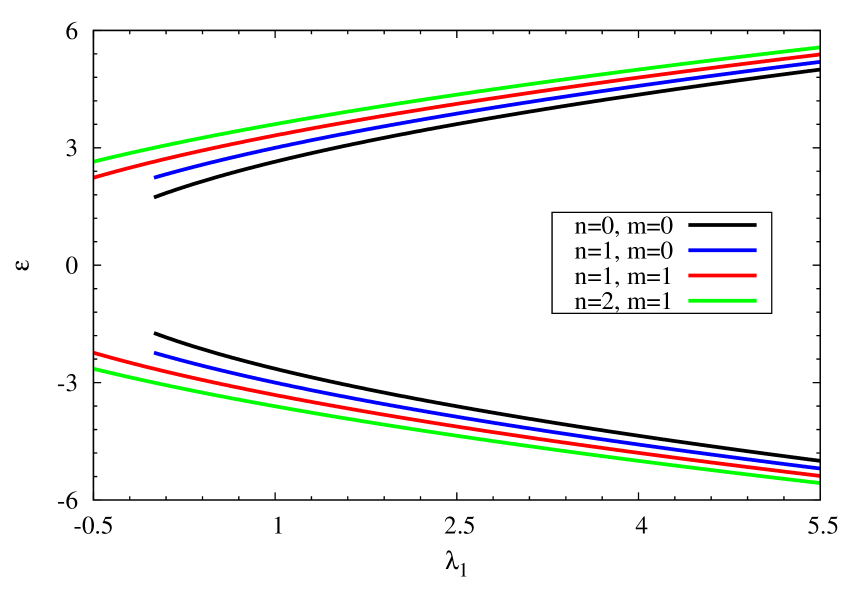
Figure 2: Plots of the energy as a function of $\lambda_{1}$ for $s=1$ and different values of $n$ and $m$.

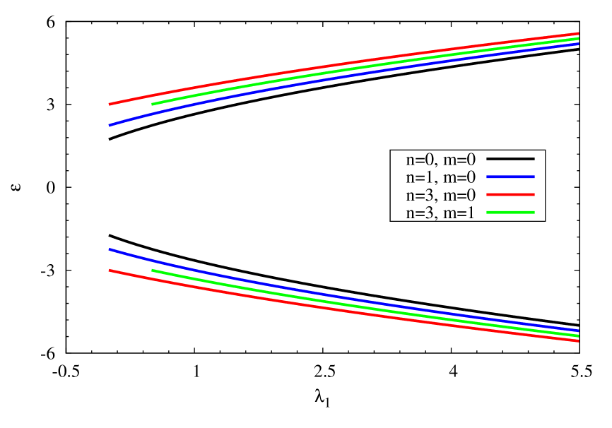
Figure 3: Plots of the energy as a function of $\lambda_{1}$ for $s=-1$ and different values of $n$ and $m$.

The unnormalized bound state wave functions are given by

$$f_{m}(\tilde{\rho}) = \tilde{\rho}^{\frac{\nu}{2}}e^{-\frac{\tilde{\rho}}{2}}F\left(-n,1+\nu,\tilde{\rho}\right)$$ (61)

$$+ \tilde{\rho}^{-\frac{\nu}{2}}e^{-\frac{\tilde{\rho}}{2}}F\left(-n,1-\nu,\tilde{\rho}\right).$$

Note that when $\left|\nu\right|\geq 1$ or equivalently when the $\delta$ interaction is absent, only the regular solution contributes for the bound state wave function ($b_{m}=0$), and the energy is given by Eq. (58).

Now, we consider the solution of Eq. (37). By performing the same steps to achieve Eqs. (58)-(59), we obtain

$$\frac{\mathcal{E}^{2}-{}M^{2}}{2\eta_{2}} =\left(2n+1+\left|m+s+s\eta_{1}\right|\right)+s\left(m+s\right)+\eta_{1}-1,$$ (62)

$$\frac{\mathcal{E}^{2}-{}M^{2}}{2\eta_{2}} =\left(2n+1-\left|m+s+s\eta_{1}\right|\right)+s\left(m+s\right)+\eta_{1}-1,$$ (63)

with unnormalized bound state wave functions given by

$$g_{m}(\tilde{\rho}) = \tilde{\rho}^{\frac{\left|\bar{\nu}\right|}{2}}e^{-\frac{\tilde{\rho}}{2}}F\left(-\bar{n},1+\left|\bar{\nu}\right|,\tilde{\rho}\right)$$ (64)

$$+ \tilde{\rho}^{-\frac{\left|\bar{\nu}\right|}{2}}e^{-\frac{\tilde{\rho}}{2}}F\left(-\bar{n},1-\left|\bar{\nu}\right|,\tilde{\rho}\right),$$

where

$$\bar{n}=\frac{1\pm\left|\bar{\nu}\right|}{2}-\frac{\bar{E}}{4\eta_{2}}.$$ (65)

If $\eta_{1}\rightarrow 0$ in Eqs. (58)-(59) and (62)-(63), we obtain

$$\frac{\mathcal{E}^{2}-M^{2}}{2\eta_{2}} = \left(2n+1+\left|m\right|\right)+ms+1,$$ (66)

$$\frac{\mathcal{E}^{2}-{}M^{2}}{2\eta_{2}} = \left(2n+1-\left|m\right|\right)+ms+1,$$ (67)

and

$$\frac{\mathcal{E}^{2}-{}M^{2}}{2\eta_{2}} =\left(2n+1+\left|m+s\right|\right)+sm-1,$$ (68)

$$\frac{\mathcal{E}^{2}-{}M^{2}}{2\eta_{2}} =\left(2n+1-\left|m+s\right|\right)+sm-1.$$ (69)

These energy levels correspond to the analogue Landau quantization for relativistic quantum dynamics of neutral fermions of spin-1/2 with magnetic moment $\mathbf{\mu}$ in the field configuration of Eq. (2).

6 Nonrelativisitic limit

Let us now examine the nonrelativistic limit of Eq. (31) by setting $\mathcal{E}={}M+\varepsilon$, with $\varepsilon\ll{}M$. The equation to be solved is

$$\frac{1}{2M}\left[\mathbf{p}+s(\mathbf{\mu}\times\mathbf{E})\right]^{2}\psi+\frac{1}{2M}\mu\sigma_{3}(\mathbf{\nabla}\cdot\mathbf{E})\psi=\varepsilon\psi.$$ (70)

Performing the same steps as for the relativistic case, we find the energy levels

$$\varepsilon=\left\{\begin{array}[]{l}\omega\left[\left(2n+1+\left|m+s\eta_{1}\right|\right)+\eta_{1}+ms+1\right],\\ \omega\left[\left(2n+1-\left|m+s\eta_{1}\right|\right)+\eta_{1}+ms+1\right].\end{array}\right.$$ (71)

where we have defined the frequency $\omega=\eta_{2}/M$. Similarly, we can also find the eigenvalues of Eq. (37). The result is given by

$$\bar{\varepsilon}=\left\{\begin{array}[]{l}\omega\left[\left(2n+1+\left|m+s+s\eta_{1}\right|\right)+s\left(m+s\right)+\eta_{1}-1\right],\\ \omega\left[\left(2n+1-\left|m+s+s\eta_{1}\right|\right)+s\left(m+s\right)+\eta_{1}-1\right].\end{array}\right.$$ (72)

If $\eta_{1}\rightarrow 0$, we obtain the energy levels corresponding to a neutral fermion of spin-1/2 with magnetic moment in the nonrelativistic regime

$$\varepsilon=\left\{\begin{array}[]{l}\omega\left[\left(2n+1+\left|m\right|\right)-ms+1\right],\\ \omega\left[\left(2n+1-\left|m\right|\right)-ms+1\right].\end{array}\right.$$ (73)

and

$$\bar{\varepsilon}=\left\{\begin{array}[]{l}\omega\left[\left(2n+1+\left|m+s\right|\right)+s\left(m+s\right)-1\right],\\ \omega\left[\left(2n+1-\left|m+s\right|\right)+s\left(m+s\right)-1\right].\end{array}\right.$$ (74)

Equations (73) and (74) can be compared, for example, with Eq. (25) of Ref. EPJC.2008.56.597 , in the absence of the spin element $s$.

7 Conclusions

We have solved the quantum dynamics of a neutral fermion with a magnetic moment $\mu$ in the presence of external electric fields. We shown that the set of first order differential equations admit isolated solutions ($E=M$, and $E=-M$). This result implies new solutions for the AC problem. We derive the second-order Dirac equation to study the motion of the particle in two situations. First, we assume that the particle describes a circular path of constant radius, and then analyze the dynamics in the full space, including the $r=0$ region. The inclusion of the $r=0$ region states that we must consider the term $\mathbf{\nabla}\cdot\mathbf{E}_{1}$ in Eq. (31), i.e., a singular term. We consider the self-adjoint extension method and show that the term $\mathbf{\nabla}\cdot\mathbf{E}_{1}$, which results in a $\delta$ function, has physical implications on the dynamics of the particle. In other words, we have verified that this term contributes for the bound state wave function and energy spectrum, and with an explicit dependence on the spin projection parameter $s$. For $\lambda_{m}=0$, case in which the $\delta$ function is absent, only the regular solution contributes for the bound state wave function. For two particular values for the self-adjoint extension parameter, $\lambda_{m}=0$ (regular solution) and $\lambda_{m}=\infty$ (irregular solution), the energies are given explicitly in Eqs. (58)-(59) and (62)-(63). In the limit $\eta_{1}\rightarrow 0$, the corresponding energy levels are analogous to Landau levels. In this limit, the dependence on s parameter is still maintained. We also have obtained these results in nonrelativistic limit.

References

- (1) M. Peshkin, H.J. Lipkin, Phys. Rev. Lett. 74(15), 2847 (1995). DOI 10.1103/PhysRevLett.74.2847
- (2) Y. Aharonov, D. Bohm, Phys. Rev. 115(3), 485 (1959). DOI 10.1103/PhysRev.115.485
- (3) Y. Aharonov, A. Casher, Phys. Rev. Lett. 53(4), 319 (1984). DOI 10.1103/PhysRevLett.53.319
- (4) Y. Aharonov, J. Anandan, Phys. Rev. Lett. 58, 1593 (1987). DOI 10.1103/PhysRevLett.58.1593
- (5) J. Anandan, Y. Aharonov, Phys. Rev. Lett. 65, 1697 (1990). DOI 10.1103/PhysRevLett.65.1697
- (6) X.G. He, B.H.J. McKellar, Phys. Rev. A 47, 3424 (1993). DOI 10.1103/PhysRevA.47.3424
- (7) H. Wei, R. Han, X. Wei, Phys. Rev. Lett. 75, 2071 (1995). DOI 10.1103/PhysRevLett.75.2071
- (8) M. Wilkens, Phys. Rev. Lett. 72, 5 (1994). DOI 10.1103/PhysRevLett.72.5
- (9) J. Anandan, Phys. Rev. Lett. 85, 1354 (2000). DOI 10.1103/PhysRevLett.85.1354
- (10) C.R. Hagen, Phys. Rev. Lett. 64(5), 503 (1990). DOI 10.1103/PhysRevLett.64.503
- (11) C.R. Hagen, Phys. Rev. Lett. 64(20), 2347 (1990). DOI 10.1103/PhysRevLett.64.2347
- (12) E.O. Silva, F.M. Andrade, C. Filgueiras, H. Belich, Eur. Phys. J. C 73(4), 2402 (2013). DOI 10.1140/epjc/s10052-013-2402-1
- (13) F.M. Andrade, E.O. Silva, M. Pereira, Phys. Rev. D 85(4), 041701(R) (2012). DOI 10.1103/PhysRevD.85.041701
- (14) F.M. Andrade, E.O. Silva, M. Pereira, Ann. Phys. (N.Y.) 339(0), 510 (2013). DOI 10.1016/j.aop.2013.10.001
- (15) E.O. Silva, F.M. Andrade, Europhys. Lett. 101(5), 51005 (2013). DOI 10.1209/0295-5075/101/51005
- (16) V. Khalilov, Eur. Phys. J. C 74(1), 1 (2014). DOI 10.1140/epjc/s10052-013-2708-z
- (17) M.S. Shikakhwa, E. Al-Qaq, J. Phys. A 43(35), 354008 (2010). DOI 10.1088/1751-8113/43/35/354008
- (18) F.M. Andrade, E.O. Silva, T. Prudêncio, C. Filgueiras, J. Phys. G 40(7), 075007 (2013). DOI 10.1088/0954-3899/40/7/075007
- (19) M. Ericsson, E. Sjöqvist, Phys. Rev. A 65, 013607 (2001). DOI 10.1103/PhysRevA.65.013607
- (20) K. Bakke, L.R. Ribeiro, C. Furtado, J.R. Nascimento, Phys. Rev. D 79(2), 024008 (2009). DOI 10.1103/PhysRevD.79.024008
- (21) K. Bakke, C. Furtado, Phys. Rev. A 80, 032106 (2009). DOI 10.1103/PhysRevA.80.032106
- (22) M. Reed, B. Simon, Methods of Modern Mathematical Physics. II. Fourier Analysis, Self-Adjointness. (Academic Press, New York - London, 1975)
- (23) B.S. Kay, U.M. Studer, Commun. Math. Phys. 139(1), 103 (1991). DOI 10.1007/BF02102731
- (24) L. Castro, A. de Castro, Ann. Phys. 338(0), 278 (2013). DOI 10.1016/j.aop.2013.09.008
- (25) L.B. Castro, A.S. de Castro, J. of Phys. A: Math. Theor. 40(2), 263 (2007). DOI 10.1088/1751-8113/40/2/005
- (26) A.S. de Castro, M. Hott, Phys. Lett. A 351(6), 379 (2006). DOI 10.1016/j.physleta.2005.11.033
- (27) M. Abramowitz, I.A. Stegun (eds.), Handbook of Mathematical Functions (New York: Dover Publications, 1972)
- (28) S. Albeverio, F. Gesztesy, R. Hoegh-Krohn, H. Holden, Solvable Models in Quantum Mechanics, 2nd edn. (AMS Chelsea Publishing, Providence, RI, 2004)
- (29) W. Bulla, F. Gesztesy, J. Math. Phys. 26(10), 2520 (1985). DOI 10.1063/1.526768
- (30) F. Gesztesy, S. Albeverio, R. Hoegh-Krohn, H. Holden, J. Reine Angew. Math. 380(380), 87 (1987). DOI 10.1515/crll.1987.380.87
- (31) L. Dabrowski, P. Stovicek, J. Math. Phys. 39(1), 47 (1998). DOI 10.1063/1.532307
- (32) R. Adami, A. Teta, Lett. Math. Phys. 43(1), 43 (1998). DOI 10.1023/A:1007330512611
- (33) F.M. Andrade, E.O. Silva, Eur. Phys. J. C 74(12), 3187 (2014). DOI 10.1140/epjc/s10052-014-3187-6
- (34) L. Ribeiro, E. Passos, C. Furtado, J. Nascimento, The European Physical Journal C 56(4), 597 (2008). DOI 10.1140/epjc/s10052-008-0681-8