Resolving Protoplanetary Disks at Millimeter Wavelengths by CARMA

Abstract

We present continuum observations at $\lambda=1.3$ mm and 2.7 mm using the Combined Array for Research in Millimeter-wave Astronomy (CARMA) toward six protoplanetary disks in the Taurus molecular cloud: CI Tau, DL Tau, DO Tau, FT Tau, Haro 6-13, and HL Tau. We constrain physical properties of the disks with Bayesian inference using two disk models; flared power-law disk model and flared accretion disk model. Comparing the physical properties, we find that the more extended disks are less flared and that the dust opacity spectral index ($\beta$) is smaller in the less massive disks. In addition, disks with a steeper mid-plane density gradient have a smaller $\beta$, which suggests that grains grow and radially move. Furthermore, we compare the two disk models quantitatively and find that the accretion disk model provides a better fit overall. We also discuss the possibilities of substructures on three extended protoplanetary disks.

1 Introduction

Circumstellar disks of young stellar objects (YSOs), particularly at the stages of Class II and III (the so-called T Tauri stars), are often called protoplanetary disks, since they are expected to form planets. These disk structures have been studied by spectral energy distribution (SED) over the past few decades (e.g., Beckwith et al., 1990; Andrews & Williams, 2005). However, in order to derive the detailed physical properties radio interferometry at (sub)millimeter wavelengths is required, since the disks are cold ($T\sim 30$ K) and small ($D\lesssim 1\arcsec$). To date about two dozen protoplanetary disks have been studied by interferometric observations with sub-arcsecond resolution (e.g, Andrews et al., 2009; Isella et al., 2009; Guilloteau et al., 2011). Recently the Atacama Large Millimeter/submillimeter Array (ALMA) started to present excellent results on transition disks, which are more evolved than protoplanetary disks, with the unprecedented sensitivity (e.g., van der Marel et al., 2013; Carpenter et al., 2014). Also, detailed studies of grain growth in protoplanetary disks beyond millimeter sizes has been carried out with the expanded Karl G. Jansky Very Large Array (JVLA) (e.g., Pérez et al., 2012). In addition, the long baseline science verification (SV) data of ALMA have recently shown unprecedented details of substructures toward HL Tau, which is one of our sample.

In the previous modeling studies of protoplanetary disks using SED or early interferometric data, a power-law disk model with sharp inner and outer edges was utilized (e.g., Beckwith et al., 1990; Mundy et al., 1996). Although the assumption is quite reasonable since the minimal-mass solar nebula shows a power-law density distribution (Weidenschilling, 1977) and numerical simulations of circumstellar disks also show a power-law density distribution (e.g., Ayliffe & Bate, 2009), it has no fundamental physics behind it. In addition, the model does not explain the difference between disk sizes detected in dust continuum (compact) and CO spectral line (extended).

The viscous accretion disk model provides a more physically motivated model, based on accretion with conservation of angular momentum (e.g., Pringle, 1981). The model has a density distribution with a form of a power-law tapered by an exponential function. One complication in this model is that the sources of viscosity in the disk are not well understood and may vary with radius and disk mass. Hughes et al. (2008) argued that the viscous accretion disk model explains both dust continuum and gas spectral line data better than the power-law disk model by qualitative comparison. In this study, we employ both flared power-law disk and flared viscous accretion disk models to investigate disk properties; we compare the two disk models in order to determine which model better fits our millimeter data. Although some studies have modeled the dust grain properties with radius in the disk using submillimeter to centimeter data (e.g., Pérez et al., 2012), we assume constant dust properties in the disk due to our relatively limited wavelength coverage.

Bayesian inference is used to determine the model parameter distributions that fit the observational data, instead of the commonly used $\chi^{2}$ method. The Bayesian approach provides a basis of probability theory to compare two models as well as to achieve parameter probability distributions, which are not given by the $\chi^{2}$ method. Although the $\chi^{2}$ method has been used widely, a couple of circumstellar disk studies have been carried out utilizing Bayesian inference (Lay et al., 1997; Isella et al., 2009; Kwon, 2009). No model comparison has been attempted for circumstellar disks so far in the Bayesian approach. Isella et al. (2010) obtained slightly smaller reduced $\chi^{2}$ values toward their $\lambda=1.3$ mm data of DG Tau and RY Tau for the accretion disk model than the power-law disk model. On the other hand, Guilloteau et al. (2011) and Kitamura et al. (2002) also utilized both models. However, their studies used thin disk models and a simple power-law temperature distribution. Our disk models are flared and our temperature distributions are obtained by a Monte Carlo radiative transfer code, which are more realistic.

In this paper, we present observational and modeling results of our protoplanetary disk survey, which has taken high angular resolution data at $\lambda=1.3$ mm and 2.7 mm using the Combined Array for Research in Millimeter-wave Astronomy (CARMA) providing high image fidelity. First, brief introductions of the targets are given in Section 2 and CARMA observations and data reduction are discussed in the following section. Afterward the two disk models of flared power-law disks and viscous accretion disks are explained, followed by observational and fitting results and discussion in Section 5. Finally, we summarize the results.

2 Targets

The circumstellar disk targets of this study (CI Tau, DL Tau, DO Tau, FT Tau, Haro 6-13, and HL Tau; Table 1) are located in the Taurus molecular cloud, a well-known, nearby star forming region. The distance has been determined by various methods (Rebull et al., 2004): e.g., star counting (e.g., McCuskey, 1938), optical extinction (e.g., Kenyon et al., 1994, $140\pm 10$ pc), parallax measurement (e.g., Hipparcos astrometric data: Bertout et al., 1999), and protostellar rotational properties (Preibisch & Smith, 1997, $152\pm 10$ pc). The measured distances to the Taurus molecular cloud are somewhat different in methods and in regions. For example, Bertout et al. (1999) reported three regions of $125^{+21}_{-16}$ pc, $140^{+16}_{-13}$ pc, and $168^{+42}_{-28}$ pc, using Hipparcos astrometric data. However, 140 pc is within uncertainties of most of the ranges, so it is adopted for all 6 targets in this study. Note that the distance affects the physical sizes and mass estimates.

Our targets were chosen from the sample of Beckwith et al. (1990), which observed 86 YSOs in the Taurus molecular cloud at $\lambda=1.3$ mm using the IRAM 30 m telescope. They were also included in the submillimeter survey at $\lambda=450$ and $850~{}\mu$m carried out by Andrews & Williams (2005) using SCUBA on the James Clerk Maxwell Telescope. On the other hand, Kenyon & Hartmann (1995) compiled published IR and optical observations with supplementary IR observations in the cloud. In addition, Furlan et al. (2009) reported $\lambda\approx 10~{}\mu$m feature strengths (equivalent width of the $10~{}\mu$m feature, EW($10~{}\mu$m)) and spectral index ($n_{13-31}$) between $\lambda=13$ and $31~{}\mu$m of T Tauri disks in the Taurus molecular cloud including our targets except HL Tau, as well as two other star forming regions using the Spitzer Space Telescope IRS data. They utilized these values to indicate dust evolution; for example, smaller $n_{13-31}$ values represent disks with more dust settlement (less flaring) and EW($10~{}\mu$m) shows the amount of small dust grains ($<5~{}\mu$m), which means that smaller EW($10~{}\mu$m) indicates more evolved dust. Selected information from the above studies is summarized in Table 1. More detailed studies have been carried out toward these targets and some selected examples are introduced in the following.

CI Tau was observed by Beckwith et al. (1990) with a continuum flux of $190\pm 17$ mJy at $\lambda=1.3$ mm. In addition, variability in optical spectra has been detected, which can be interpreted as a temporary obscuration of a local hot region (Smith et al., 1999). Andrews & Williams (2007) observed CI Tau using the Submillimeter Array (SMA) at $\lambda=880~{}\mu$m with a moderate angular resolution ($>1^{\prime\prime}$). By model fitting of SED data and visibility data averaged in annulus, they constrained physical properties such as density and temperature distributions, size, and mass. Guilloteau et al. (2011) also studied this target by about $0.5^{\prime\prime}\times 0.3^{\prime\prime}$ angular resolution data at two wavelengths of the Plateau de Bure Interferometer (PdBI) and two disk models: power-law and accretion disk models.

DL Tau has been detected with a continuum flux of $230\pm 14$ mJy by IRAM observations (Beckwith et al., 1990). It has also been detected in the $\textrm{CO}~{}J=2\rightarrow 1$ line, and the velocity field was shown (e.g., Koerner & Sargent, 1995). Simon et al. (2000) studied the kinematics using PdBI data in $\textrm{CO}~{}J=2\rightarrow 1$. They showed that the disk is in Keplerian rotation and estimated the protostellar mass as $0.72\pm 0.11$ M_⊙ assuming the inclination determined by the continuum image ($49\pm 3\arcdeg$). Kitamura et al. (2002) has studied the disk structure by fitting SEDs and Nobeyama Millimeter Array data taken at $\lambda=2$ mm with $1^{\prime\prime}$ resolution. They employed a viscous accretion disk as well as a power-law disk model. Andrews & Williams (2007) also studied the DL Tau disk structure using SMA data at $\lambda=1.3$ mm with about $2^{\prime\prime}$ resolution. This target was also studied by Guilloteau et al. (2011) using PdBI.

DO Tau has a continuum flux of $136\pm 11$ mJy in the Beckwith et al. (1990) observations. Koerner & Sargent (1995) have reported $\textrm{CO}~{}J=2\rightarrow 1$ observational results . The line profile has a much broader feature in the blueshifted region than in the redshifted region, which indicates that it needs infall and bipolar outflow components. DO Tau is also one of the sample in the studies of Kitamura et al. (2002).

FT Tau has a continuum flux measured in Beckwith et al. (1990) of $130\pm 14$ mJy at $\lambda=1.3$ mm. In previous survey observations at optical wavelengths, however, the spectral type of FT Tau was not determined probably due to an undetermined luminosity, although the surveys included the target. Therefore, there is no good estimate of protostellar mass and age, which are normally determined by its effective temperature and luminosity. Robitaille et al. (2007) reported wide ranges of stellar parameters by SED fitting: for example, protostellar temperature between 3060 and 5013 K and mass between 0.11 and 2.03 M_⊙. Andrews & Williams (2007) observed FT Tau with an angular resolution of $1.7^{\prime\prime}\times 1.1^{\prime\prime}$ at $\lambda=880~{}\mu$m using SMA. Although they did not resolve the disk structure, they constrained disk properties by model fitting with the data and SEDs. The study of Guilloteau et al. (2011) using PdBI included this target taken at about $0.5^{\prime\prime}\times 0.3^{\prime\prime}$ angular resolution.

Haro 6-13 has been detected with a continuum flux of $124\pm 13$ mJy by Beckwith et al. (1990). Schaefer et al. (2009) observed the target in CO $J=2\rightarrow 1$ and $J=1\rightarrow 0$ as well as $\lambda=1.3$ mm and 2.7 mm continuum using PdBI. They estimated the protostellar mass as $1.0\pm 0.15$ M_⊙, based on the rotational velocity field. They discussed that the difference from the mass estimated by the evolutionary track on the HR diagram ($\sim 0.6$ M_⊙) may be due to limited number of channel maps for the CO data model fitting. The PdBI data of Schaefer et al. (2009) were also used in Guilloteau et al. (2011).

HL Tau has been studied very broadly over the last two decades, as it is a bright T Tauri star. It has been studied by submillimeter and millimeter imaging of interferometers (e.g., Kwon et al., 2011, and references therein), as well as molecular line observations. In particular, by a modeling of the viscous accretion disk model to millimeter CARMA data and SED data, we found that HL Tau experiences stratified grain settlement and has an outer disk region gravitationally unstable (Kwon et al., 2011). In fact, this paper uses the same data set of HL Tau but we employ two disk models and a better temperature distribution. HL Tau has also been studied by PdBI (Guilloteau et al., 2011) and has recently been observed by ALMA at three wavelengths (ALMA Band 3, 6, and 7) with an excellent angular resolution down to $\sim 0.02^{\prime\prime}$.

3 Observations and Data

We carried out a survey of protoplanetary disks using CARMA, which is a heterogeneous array consisting of six 10.1-m, nine 6.4-m, and eight 3.5-m antennas. For this project the 3.5-m antennas were not used for imaging. All targets were observed in A and/or B configurations (see Table 2) at $\lambda=1.3$ mm and/or 3 mm, which provide high angular resolution better than $0.3$″ at $\lambda=1.3$ mm. Table 3 provides details on the final combined data, their synthesized beam sizes and noise levels.

In addition to the most extended A and B configurations, we have observed the protoplanetary disks in C and D configurations, in order to detect large scale structures as well as small scales. The highest angular resolution (the smallest synthesized beam size) is $\sim$0.13″ at $\lambda=1.3$ mm toward HL Tau. The angular resolutions for the other targets are a bit less ($\sim$0.3″). The uv coverage of our data are summarized in Table 3. As shown in the table, the minimum uv distance is at most 17 kilo-wavelengths, which means that our large scale sensitivity is at least 10 arcseconds. As the target disks are less than a few arcseconds in size, there is no resolving-out flux issue in the study, from which interferometric observations typically suffer for extended targets.

The largely extended arrays (A and B configurations) require stable atmospheric conditions due to long baselines. It is challenging to obtain such good weather conditions even at the CARMA site. To verify our data quality, therefore, we have observed an additional calibrator (a test calibrator) with a gain calibrator. Since a test calibrator is chosen to be a point source nearby our targets, data quality after applying gain solutions can be examined by the test calibrator’s shape and flux. All of our A and B configuration data and some of the compact array data have such a test calibrator. Most of our data have built a point or point-like image of a test calibrator, which means successful calibration. Here “point-like” means that the deconvoluted size of a test calibrator is less than half of a synthesized beam in both major and minor axes. A few of the worst data sets have a test calibrator size comparable to the synthesized beam and those sets are indicated in Table 2. In addition, we examined the flatness of the uv amplitude slopes of the gain calibrators. Since uv data are the Fourier transform of an image, a gain calibrator of a point source should have a flat amplitude versus uv distance. If it is not achieved, i.e., amplitudes at long uv distance regions (small scales, central regions) drop, the target data are likely to be biased, resulting in an apparent shallower gradient of density and/or temperature. All of our data sets have a flat amplitude slope of gain calibrators after calibration, except a data set taken in B configuration at $\lambda=1.3$ mm toward DO Tau, which has about 25% variation in the middle. However, it does not seem to affect the results significantly, as the variation is acceptable in magnitude and is positioned in the middle of uv coverage. Therefore, we include that data as well with caution, in order to have long baseline data.

CARMA itself has a special technique for calibration of atmospheric perturbation, called CARMA Paired Antenna Calibration System (CPACS) (Lamb et al., 2009). In large antenna spacings such as A and B configurations, the 3.5 m antennas are paired with boundary 10.4 m or 6.1 m antennas, which are elements of long baselines. The 3.5 m antennas are always observing a calibrator at 30 GHz, while the other antennas are observing science targets and calibrators. During the calibration of data, the phase of the 3.5 m antenna gain solution is used to correct the phase delay (phase difference) caused by short atmospheric perturbations ($\sim$4–20 seconds) on the paired antennas. Since visibility phase depends on time delay and wavelengths/frequencies, the phase of the gain solution is scaled by the ratio of observation frequencies to 30 GHz. The A configuration data of HL Tau at $\lambda=1.3$ mm and the A configuration data of FT Tau at $\lambda=2.7$ mm are calibrated using CPACS. The calibrators used for CPACS are separated from HL Tau and FT Tau by $9\arcdeg$ and $13\arcdeg$, respectively, and the improvement of calibrated data is about 10–20% in terms of image noise levels and the size, flux, and peak intensity of test calibrators.

We obtained two wavelength data ($\lambda=1.3$ mm and 2.7 mm) in order to better constrain the dust properties. The properties constrained by multi-frequency data mainly depend on absolute flux calibration. To minimize the bias induced by flux calibration uncertainty, a good flux calibrator (e.g., Uranus) was used (Table 2). In addition, gain calibrator fluxes of all tracks have been compared with each other in the time basis. Rapid variation of gain calibrator fluxes (e.g., 50% increase or decrease within a few days) is unrealistic, although quasar gain calibrators are intrinsically variable. For comparison, the CARMA flux catalog and the SMA calibrator list have been taken into account, as well as the gain calibrator values bootstrapped from flux calibrators. In addition, different array-configuration data of the same targets have been compared at common uv distances. Sub/millimeter dust emission from T Tauri disks is not variable over a period of a few years, so amplitudes at common uv positions should be comparable even in different configuration arrays. Actually, this comparison is a crucial step when combining various array-configuration data. As a result, we presume absolute flux calibration uncertainty of our T Tauri disk data is less than the uncertainty assumed in other studies, which use only one or two tracks in an array-configuration for each frequency data: 10% at $\lambda=1.3$ mm and 8% at $\lambda=2.7$ mm (e.g., Kwon et al., 2011).

We also considered proper motions of our targets when combining our data, as they have been taken over a few year period. However, since proper motions of all targets have not yet been well estimated, we decided not to correct them blindly. Instead, we estimated the proper motion based on the data themselves. In the case of Haro 6-13, whose peaks show an offset in the data set, we matched the peak positions. As a result, we shifted the 3 mm data sets by (R.A., Dec.) = ($0.0105^{\prime\prime}$, $0.055^{\prime\prime}$). In addition, for HL Tau, whose data have the highest angular resolution and whose proper motion is well measured, we compensated for the proper motion (Kwon et al., 2011).

MIRIAD (Sault et al., 1995) has been employed to calibrate and map data. Individual tracks have been calibrated and verified separately then combined in the invert-Fourier transform step to make maps. The sensitivity and emphasized scales in the maps depend on the visibility data weighting scheme. Natural weighting gives the highest signal-to-noise and the worst angular resolution, since visibility data points are sparse at large uv distances and visibilities at larger uv distances are noisier due to atmospheric turbulence. On the other hand, uniform weighting emphasizes small scales best although the signal-to-noise is worst. For intermediate weighting, Briggs introduced a robust parameter (Briggs, 1995): 2 of the parameter for weighting close to the natural weighting and -2 close to the uniform weighting. In order to have small structures reasonably emphasized, the weighting scheme with a robust value of 0 has been applied.

4 MODELING

We employ two disk models to estimate disk physical parameters: a viscous accretion disk model (e.g., Pringle, 1981) and a power-law disk model (e.g., Beckwith et al., 1990). The outer boundary of the two disk models are described differently. While a sharp outer radius is associated with the power-law disk model, a characteristic radius is introduced in the viscous accretion disk model, which has a power-law density structure tapered by an exponential function. We also consider vertical structures for investigating disk thickness and flare degree. For our models, we use cylindrical coordinates, and the disk models are axisymmetric. Therefore, the physical properties are expressed in $R$ and $z$ coordinates: e.g., density structures $\rho(R,z)$. On the other hand, $r$ indicates a direct distance from the disk center, i.e., $r^{2}=R^{2}+z^{2}$. The model emission is calculated with a logarithmic radial grid to ensure accurate values in the inner region of the disk.

4.1 Power-law Disk Model

The power-law disk model has a power-law density distribution with a sharp edge,

$$\rho(R,z) = \rho(R,0)~{}\textrm{exp}[{-(z/H(R))^{2}}]$$ (1)

$$= \rho_{0}\Big{(}\frac{R}{R_{0}}\Big{)}^{-s}\textrm{exp}[{-(z/H(R))^{2}}],$$

where $H(R)$ is a scale height along radius set by a power-law function:

$$H(R)=b_{t}H_{0}\Big{(}\frac{R}{R_{0}}\Big{)}^{h}.$$ (2)

Here $H_{0}=(2kR_{0}^{3}T_{0}/GM_{*}\bar{m})^{0.5}$ is the hydrostatic equilibrium case between the vertical component of the protostellar gravity and the local pressure of $T(R_{0},0)=T_{0}$. We ignore self gravity of the disk mass and assume that dust temperature and gas kinetic temperature are the same. In the $H_{0}$ expression, $k$ is the Boltzmann’s constant, G is the gravitational constant, $M_{*}$ is the central protostellar mass, and $\bar{m}$ is the mean molecular mass: $\bar{m}=\mu m_{H}=2.4m_{H}$. Note that disks in the hydrostatic equilibrium and in the optically thin condition have $b_{t}=1$ and $h=3/2-q/2\approx 1.25$, where $T(R,0)\propto R^{-q}$.

As the surface density is obtained by the integration of the density distribution in $z$, the surface density is also a power law with a power index of $p=s-h$:

$$\Sigma(R) = \int_{-\infty}^{\infty}\rho(R,z)dz$$ (3)

$$= \rho(R,0)\sqrt{\pi}H(R)$$

$$= \rho_{0}\sqrt{\pi}b_{t}H_{0}\Big{(}\frac{R}{R_{0}}\Big{)}^{-p}.$$

In this model we also have a sharp inner radius ($R_{in}$) in addition to the outer radius ($R_{out}$). Therefore, $\rho_{0}$ is expressed with a disk total mass ($M_{disk}$),

$$M_{disk} = \int^{R_{out}}_{R_{in}}\int^{\infty}_{-\infty}\rho(R,z)dz~{}2\pi R~{}dR$$

$$= \rho_{0}\frac{2\pi^{1.5}R_{0}^{2}b_{t}H_{0}}{2-p}\Big{[}\Big{(}\frac{R_{out}}{R_{0}}\Big{)}^{2-p}-\Big{(}\frac{R_{in}}{R_{0}}\Big{)}^{2-p}\Big{]}$$

$$\rho_{0} = M_{disk}\frac{2-p}{2\pi^{1.5}R_{0}^{2}b_{t}H_{0}}\Big{[}\Big{(}\frac{R_{out}}{R_{0}}\Big{)}^{2-p}-\Big{(}\frac{R_{in}}{R_{0}}\Big{)}^{2-p}\Big{]}^{-1}$$ (4)

Although we consider a power-law temperature distribution for the disk scale height, we use a temperature distribution calculated in a given disk structure by the RADMC 3D code (Dullemond & Dominik, 2004) for more realistic modeling with a temperature gradient along the vertical direction. However, we did not update the scale height based on the calculated temperature distribution. This decoupling of the disk structure from the temperature distribution is justified, because dust grains settle to the mid-plane rather than mix with gas as they grow (e.g., Andrews et al., 2009).

The RADMC 3D code provides two dimensional temperature distributions, but it requests a large number of photons for a smoothly varying distribution particularly in the case of thin disks with a high optical depth. Therefore, instead of simply using the temperature distributions out of the RADMC 3D code, we make a functional form weighting two functions that fit to the mid-plane ($T_{m}$) and surface temperature distributions ($T_{s}$),

$$T(R,z)=WT_{m}(R,0)+(1-W)T_{s}(r).$$ (5)

Based on qualitative comparisons, we chose the weighting function $W=\textrm{exp}[-(z/H(R))^{2}]$.

The dust opacity spectral index $\beta$ is one of the most interesting parameters in this study, which represents dust grain sizes (Draine, 2006): $\kappa_{\nu}=\kappa_{0}(\nu/\nu_{0})^{\beta}$. Indeed, in order to constrain $\beta$, we fit the two wavelength data simultaneously. Therefore, we assume $\kappa_{0}=0.01$ cm² g^-1 at 230 GHz and $\beta$ is determined between $\lambda=1.3$ mm and 2.7 mm. The $\kappa_{0}$ is based on the case of ice mantle grains following a MRN size distribution (Mathis et al., 1977) in Ossenkopf & Henning (1994). In addition, we assume a gas-to-dust mass ratio of 100. The assumed $\kappa_{0}$ corresponds to the case of $\kappa_{\nu}=0.1(\nu/1200~{}GHz)^{\beta}$ with $\beta=1.39$ (e.g., Hildebrand, 1983; Beckwith & Sargent, 1991). The uncertainty of $\kappa_{0}$ is large, around factor of two (Ossenkopf & Henning, 1994). For the opacity as an input of RADMC when determining disk temperature distributions we simply consider the combination of an opacity curve at infrared wavelengths in the case of silicate-carbon grains in the MRN size distribution and a power-law at millimeter wavelengths.

4.2 Viscous Accretion Disk Model

In addition to the power-law disk model, we utilize the viscous accretion disk model for fitting our data. The viscous accretion disk model has a density distribution of a power-law tapered by an exponential function (e.g., Pringle, 1981),

$$\rho(R,z) = \rho_{0}\Big{(}\frac{R}{R_{c}}\Big{)}^{-s}\textrm{exp}\Big{[}\Big{(}\frac{R}{R_{c}}\Big{)}^{2-s+h}\Big{]}~{}\textrm{exp}\Big{[}-\Big{(}\frac{z}{H(R)}\Big{)}^{2}\Big{]}.$$ (6)

The viscous accretion disk model is expressed as the surface density distribution (e.g., Andrews et al., 2009),

$$\Sigma(R) = \int_{-\infty}^{\infty}\rho(R,z)dz$$ (7)

$$= \rho_{0}\sqrt{\pi}b_{t}H_{0}\Big{(}\frac{R_{c}}{R_{0}}\Big{)}^{h}\Big{(}\frac{R}{R_{c}}\Big{)}^{-s+h}\textrm{exp}\Big{[}-\Big{(}\frac{R}{R_{c}}\Big{)}^{2-s+h}\Big{]}$$

$$= \Sigma_{0}\Big{(}\frac{R}{R_{c}}\Big{)}^{-\gamma}\textrm{exp}\Big{[}-\Big{(}\frac{R}{R_{c}}\Big{)}^{2-\gamma}\Big{]},$$

where $R_{c}$ is a characteristic radius. Note that $\Sigma_{0}=\rho_{0}\sqrt{\pi}H(R_{c})$ and $\gamma=s-h$. Like the power-law disk model, we decouple the scale height distribution from the temperature distribution, and the density distribution is expressed with the total disk mass,

$$M_{disk} = \int_{R_{in}}^{\infty}\int_{-\infty}^{\infty}\rho(R,z)dz~{}2\pi R~{}dR$$

$$= \rho_{0}\frac{2\pi^{1.5}R_{c}^{2}H(R_{c})}{2-\gamma}\textrm{exp}\Big{[}-\Big{(}\frac{R_{in}}{R_{c}}\Big{)}^{2-\gamma}\Big{]}$$

$$\rho_{0} = M_{disk}\frac{2-\gamma}{2\pi^{1.5}R_{c}^{2}H(R_{c})}\textrm{exp}\Big{[}\Big{(}\frac{R_{in}}{R_{c}}\Big{)}^{2-\gamma}\Big{]}.$$ (8)

Everything except the density distribution is set in the same way to the power-law disk model. Note that the characteristic radius ($R_{c}$) is introduced instead of the outer radius ($R_{out}$).

4.3 Model Parameters

There are 7 free parameters for each disk model: $s$, $\beta$, $M_{disk}$, $R_{in}$, $R_{out}$ (or $R_{c}$), $\theta_{i}$, and $PA$. In addition, there are two parameters related to the disk scale height, $h$ and $b_{t}$, which are weakly constrained by the observations and will be handled as “controlled parameters” in the fitting. The $\theta_{i}$ is an inclination angle of a disk (a face-on disk with $\theta_{i}=0\arcdeg$) and $PA$ is a position angle of a disk measured eastward from the north. The $R_{out}$ and $R_{c}$ are for the cases of power-law disk and viscous accretion disk models, respectively. For the viscous accretion disk model, an outer disk radius is not employed. However, the modeling disks are cut off at 5 $R_{c}$ due to limitation in image size and for simplicity in integration. Some modeling studies of circumstellar disks have presumed sublimation radii of dust grains (e.g., Andrews et al., 2009), but it is possible that inner radii ($R_{in}$) are determined by other effects such as an unresolved binary companion, formed planets, etc. Therefore, we leave the inner radii as a free parameter, but fitted values can be model-dependent and are likely unreliable due to systematic uncertainties in the observation, primarily the resolution.

The sign of inclinations are determined by our spectral line data in CO, which were included in our observations. We only detected CO in data from the C and D configurations, which traces the bipolar outflows as well as a disk structure. This allowed us to estimate the disk inclination, at least the sign. CI Tau and FT Tau, which we have not detected any CO, are set to have a plus sign of inclination. All the inclination signs are consistent with previous studies (e.g., Guilloteau et al., 2011).

The two controlled parameters, $b_{t}$ and $h$, are used to investigate the disk vertical structure. As shown in equation 2, $b_{t}$ and $h$ are disk scale heights with respect to the hydrostatic equilibrium cases and disk flare indexes. In order to figure out whether preferred disks are thin or thick and more or less flared, we carry out 25 separate models for each target: $b_{t}=\{0.6,0.8,1.0,1.2,1.4\}$ and $h=\{0.95,1.10,1.25,1.40,1.55\}$. We adopted the 25 cases instead of having them as two additional free parameters for maximizing the efficiency of our modeling without losing our study goals.

4.4 Model Fitting Procedures

First, a temperature distribution is obtained by the RADMC 3D code in a given disk structure and fitted as described in Section 4.1. Then, a disk model is built in two dimensional logarithmic grids by solving the radiative transfer equation numerically along the line of sight. Note that the disk inclination is applied when constructing the disk model, so the disk model must be two dimensional and the radiative transfer equation is numerically integrated along the third axis, line of sight. No optically thin nor Rayleigh-Jeans approximations are assumed. Afterward, disk images are made by interpolations of the disk models in two dimensional linear pixels. The center positions and position angles (PAs) of the disks are applied when making the disk images.

The disk images are multiplied by three different normalized primary beams, which correspond to three different types of baselines in CARMA: 10.4 m–10.4 m antennas, 10.4 m–6.1 m antennas, and 6.1 m–6.1 m antennas. These three primary beam corrected images are Fourier-transformed into model visibility maps. Then, the actual model visibilities are sampled in the uv coverage of observational data by bi-linear interpolation of the model visibility maps. Image pixel sizes and image sizes are selected to obtain reasonable pixel sizes and uv coverage of visibility maps. For example, an image pixel size of 9 AU and an image size of 1024 pixel by 1024 pixel are used, which provide uv coverage up to 1600 $k\lambda$ (uv range: -1604 to +1604 $k\lambda$) and a visibility map pixel of about 3.1 $k\lambda$, based on the Nyquist theorem: for example, the uv range $\Delta_{uv}=1/2\delta_{image}$, where $\delta_{image}$ is the image pixel size.

Model fitting is done by comparing observational data with the model data sampled along the observational uv coverage in Bayesian inference (e.g., Gilks et al., 1996; MacKay, 2003). Bayesian inference allows us to obtain the probability distribution of disk properties ($m$) with given data $D$ and a given disk model $H$: $P(m\mid D,H)$,

$$P(m\mid D,H)=\frac{P(D\mid m,H)P(m\mid H)}{P(D\mid H)}.$$ (9)

Here $P(m\mid D,H)$ is called the posterior probability, $P(D\mid m,H)$ the likelihood, $P(m\mid H)$ the prior, and $P(D\mid H)$ the evidence. The evidence is also called the marginal likelihood, which is used to compare multiple models, since $P(D\mid H)=\int dmP(D\mid m,H)P(m\mid H)\approx\Sigma~{}P(D\mid m,H)P(m\mid H)$. Gaussian functions are employed for the likelihood, since noise of interferometric data is a normal distribution, $\prod_{i}\textrm{exp}[-(D_{i}-M_{i})^{2}/2\sigma_{i}^{2}]$. Theoretical uncertainties of interferometric visibility points are typically estimated as $\sigma=({2k}/{A\eta})\sqrt{{T_{1}T_{2}}/{2t_{int}\Delta\nu}}$ (e.g., Thompson et al., 2001), where k is Boltzmann’s constant, A is antenna area, $\eta$ is the efficiency of the antenna surface and correlator quantization, $T_{1}$ and $T_{2}$ are system temperatures of antennas corresponding to the baseline, $\Delta\nu$ is bandwidth, and $t_{int}$ is integration time. However, the uncertainties do not represent decorrelation of atmospheric turbulence, which depends on $\it{uv}$ distance. Therefore, instead we use the standard deviation of the imaginary components of self-calibrated gain calibrator data, which are generally a few times larger than the theoretical estimate (Kwon et al., 2011). Individual wide bandwidth windows ($\Delta\nu\sim 500$ MHz) are averaged and considered a visibility point. The central channel frequency of the window is used for computing its uv distance in units of wavelength. As the data are real numbers in image space, i.e., the uv coverage is symmetric at the phase center, the symmetric data points are added to the sample. In addition, the real and imaginary components of complex visibility data are regarded as independent data.

Searching distributions of model parameters by the Metropolis Hastings method has two parts. The first part is finding a convergence region of parameters. For a better performance, we start with 8 initial conditions, which are randomly generated. After running for a while, the initial conditions converge into a parameter set (normally two sets with different signs of inclination angles). Annealing is also used to accelerate the convergence. We start a fresh run from the convergent parameter set of the expected inclination sign (refer to Section 4.3) with a smaller standard deviation of the proposal Gaussian functions, for each combination of $b_{t}$ and $h$, 25 in total for each target. The smaller standard deviation of the proposal functions are set to have an acceptance rate of about 10–50 %. The GASDEV subroutine of the Numerical Recipes using the Box-Muller method is used to produce random numbers in the Gaussian distribution (Press et al., 1996).

5 Results and Discussion

5.1 Combined Data and Images

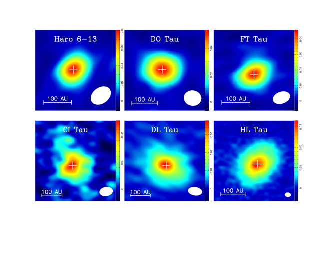
Figure 1: Protoplanetary disk images in $\lambda=1.3$ mm continuum. The color scales are in units of Jy beam^-1, and the synthesized beams and the 100 AU bars are marked at the bottom of each panel.

Figure 1 shows $\lambda=1.3$ mm continuum images of the six protoplanetary disks; a physical scale bar of 100 pc and the data angular resolution (synthesized beam) are marked. Note that the three disks in the bottom panels (CI Tau, DL Tau, and HL Tau) are extended, while the three disks in the upper panels (Haro 6-13, DO Tau, and FT Tau) are relatively compact. In addition, CI Tau has a weak non-axisymmetric feature north-north-east to south-south-west.

The continuum noise levels that we achieved after combining all configuration data are listed in Table 3 with disk total fluxes. In addition, Table 3 has disk center positions estimated by a Gaussian fit (the IMFIT task of MIRIAD). Table 1 has phase center coordinates, so one can simply compute the actual disk centers: e.g., HL Tau, R.A. (J2000) = 04:31:38.418, Dec. (J2000) = +18:13:57.37.

Figure 2 presents observational visibilities of six targets averaged in annulus with the best fitting model overlaid: the solid and dashed lines indicating accretion disk and power-law disk models, respectively. The dust opacity spectral indexes at the bottom of each panel have been calculated in the optically thin assumption and the Rayleigh-Jeans approximation: $\beta\approx\textrm{log}(F_{1mm}/F_{3mm})/\textrm{log}(\nu_{1mm}/\nu_{3mm})-2$. The $\beta$ values from our modeling without such assumption and approximation are addressed later. Open squares and open triangles mark $\lambda=1.3$ mm and 2.7 mm data, respectively. The error bars are the standard error of the mean: $\sqrt{\Sigma\sigma_{i}^{2}/N^{2}}$, where $\sigma_{i}^{2}$ is the variance of a visibility data point in a annulus calculated from its $T_{sys}$ and N is the total number of data in the annulus. Absolute flux calibration uncertainty is not applied for the plots. As shown, the two models are fitting observational data well. Note that since the viscous accretion disk model does not have an outer radius, there are no bump features at around $200-300~{}k\lambda$, corresponding to about $1^{\prime\prime}$.

Although the $\beta$ values of the figure are simply calculated and not from our modeling, it is worthy of noting the weak relative variations along uv distance, which can be used for studying grain size distributions. In general, recent studies reported that protoplanetary disks have larger grains in the inner regions (e.g., Guilloteau et al., 2011; Pérez et al., 2012; Trotta et al., 2013). Observations with higher angular resolution and sensitivity at multiple wavelengths are required to investigate the spatial distributions of dust grains. We do not intend to study the grain size distributions in this paper and simply assume a constant $\beta$.

5.2 Fitting Results

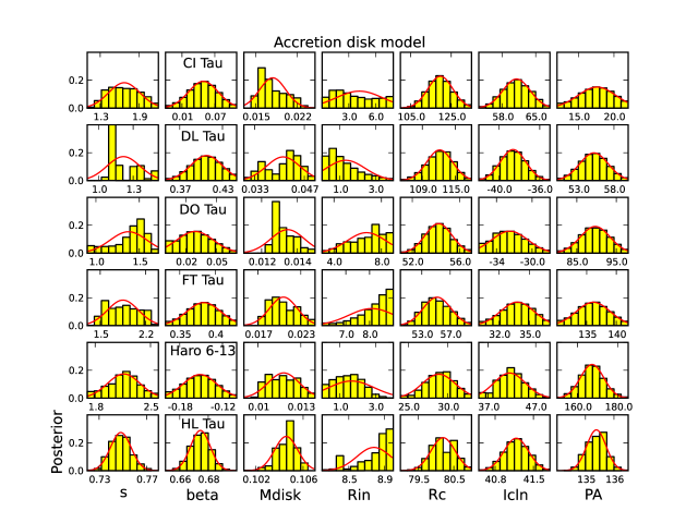
Figure 3: Posterior distributions of accretion disk model parameters fitting 6 disk data. Target names are indicated in the $\beta$ panels, the second column from the left. The $M_{disk}$ is in units of $M_{\sun}$, $R_{in}$ and $R_{out}$ are in AU, and inclination and position angles are in degree.

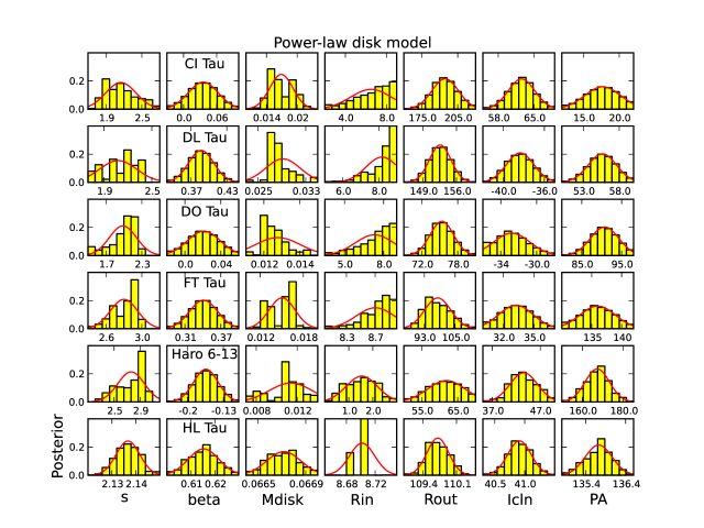
Figure 4: Posterior distributions of power-law disk model parameters fitting 6 disk data.

We have carried out two flared disk models: viscous accretion disk and power-law disk models. As described in Section 4, we have 7 free parameters and two controlled parameters for the vertical structures (5 disk thickness $b_{t}$ and 5 flare index $h$ values). The fitting results are presented in Table 4 and Figures 3 and 4. The 25 cases of the controlled parameters are combined in order to see the overall parameter ranges, as they have been sampled with the same Gaussian proposal function (Section 4.4).

We did not use any priors obtained from the images of the targets except the center positions and the inclination signs. We tested the center positions determined by a Gaussian fit of the IMFIT task in MIRIAD and the ones manually determined, based on the intensity peak positions. The offset values by the simple Gaussian fit have been chosen (Table 3), as they give higher posteriors.

The fitting results are listed in Table 4 and the posterior distributions of parameters in individual targets are presented in Figure 3 and 4. The table values are the means and standard deviations of individual parameters in the marginal probability distributions. The solid lines of Figure 3 to 4 indicate normal distributions. As shown, most parameters have a normal distribution posterior, and hence well defined values and deviation.

The exception is the inner radius. The inner radius was fit over a range from 1.3 to 9 AU because none of the disks showed an inner hole or central depression of emission at our best 18 AU resolution. The resulting fits show weak dependence on inner radius. The statistical uncertainties in Table 4 do not account for the systematics of increased atmospheric de-coherence on the longest baseline which are biased toward blurring the central disk emission. The inner radius for HL Tau, the source with the best resolution and signal-to-noise, may represent a flattening of the surface density distribution within 10 AU rather than a central hole (i.e. ALMA SV data).

The volume density distribution index ($s$) of the power-law disk model is between $\sim$2.0 to $\sim$2.8, which corresponds to a surface density index ($p$) between $\sim$0.4 and $\sim$1.8 when the best flare index values are adopted ($p=s-h$ in Section 4). On the other hand, the $s$ values of the accretion disk model are in a range of 0.7 to 2.2, which are converted into $\gamma$ expressing the surface density distribution ($\gamma=s-h$) of -0.2 to 1.1, as shown in Table 4. Such a large range of $\gamma$ has been reported by previous studies (Isella et al., 2009; Andrews et al., 2009).

The dust opacity spectral index $\beta$ appears to be constrained very closely in the two models. This is expected because $\beta$ is sensitive to the difference of flux densities at two wavelengths. $\beta$ of our sample disks ranges from -0.15 to 0.70 and half of them are around 0, which can be interpreted as grain growth. $\beta$ of younger Class 0 YSOs is around 1 (Kwon et al., 2009), so grains may grow with object evolution. This is still valid for DL Tau, FT Tau and HL Tau, since they have $\beta$ smaller than 1. Note that the possible error of $\beta$ due to the absolute flux calibration uncertainties (10% at $\lambda=1.3$ mm and 8% at $\lambda=2.7$ mm; refer to Section 3) are about 0.25.

Disk masses are 0.01–0.10 M_⊙. Compact disks (DO Tau, FT Tau, Haro 6-13) tend to have smaller masses. However, disk masses are distributed in a large range, among which HL Tau has the largest mass. Note that the disk masses have a large uncertainty mainly because $\kappa_{0}$ has a factor of two uncertainty (e.g., Ossenkopf & Henning, 1994). In addition, the stellar luminosity affects the disk mass, as it sets the dust temperature. However, disk masses are not so sensitive to the stellar luminosity due to the low power index and the high optical depth along radius. Note that the derived temperature distributions for our modeling are calculated by the Monte-Carlo radiative transfer code of RADMC 3D.

The disk sizes (characteristic and outer radii) are well constrained in both models: $R_{c}\approx 30$–120 AU and $R_{out}\approx 60$–200 AU. The characteristic radius of the accretion disk model is where the disk density distribution changes from the power-law dominant region to the exponential dominant region (Equation 6). Comparing the surface density equation of our accretion disk model with a similarity solution of viscous accretion disks and considering the mass flow equation (e.g., Andrews et al., 2009; Hartmann et al., 1998; Pringle, 1981), the characteristic radius can express the transitional radius $R_{t}$, where the bulk flow direction changes from inward to outward to conserve angular momentum (e.g., Equation A9 in Andrews et al., 2009):

$$R_{t}=R_{c}\Big{[}\frac{1}{2(2-\gamma)}\Big{]}^{1/(2-\gamma)}.$$ (10)

The $R_{t}$ of our sample disks are in a range of about 15 to 60 AU, as listed in Table 4.

The two geometrical parameters, inclination ($\theta_{i}$) and position angle (PA), are the two best constrained. The values are consistent with previous high angular resolution observations. In addition, they are consistent in both models, so model-independent. We originally did not limit the inclination sign based on the known bipolar outflow directions of our targets in the modeling. However, for the final modeling results, we have chosen the inclination sign in agreement with the bipolar outflow direction and/or previous studies (e.g., Guilloteau et al., 2011).

Five of our disks were also observed and fit to power-law and accretion disk models by Guilloteau et al. (2011). Disk inclination and position angles agree fairly well (accounting for the difference in definition of position angle) but other disk parameters show only broadly similar trends, without detailed agreement. For HL Tau and Haro 6-13, our angular resolution, which is a factor of 3-4 higher, is the likely reason for the difference. For CI Tau, where the resolutions of the observations are nearly the same, the fitted disk parameters, $R_{c}$, $\gamma$, $R_{out}$, and $p$, are similar, but generally outside of the statistical uncertainties by more than 2$\sigma$. Guilloteau et al. (2011) assume a simple $R^{-0.4}$ power-law for the radial temperature variation which may be responsible in part for the difference. However, it is likely that both analysis are more limited by the sensitivity and angular resolution of the observations than is reflected in the statistical uncertainties. This is a cautionary note for all disk modeling to date.

5.3 Model Comparison

First, we compared posteriors of the two models. Bayesian inference provides a way for model comparison; models can be compared by evidence, which is the integration of likelihood times prior over the whole possible parameter space of a model (e.g., MacKay, 2003). We set the prior as well as the number of free parameters the same for the two models (uniform priors over the same ranges), so we just need to integrate likelihood. The likelihood integration can be estimated by the best likelihood times the posterior accessible volume:

$$K = \frac{P(D\mid H_{A})}{P(D\mid H_{P})}$$ (11)

$$= \frac{\int dmP(D\mid m,H_{A})P(m\mid H_{A})}{\int dmP(D\mid m,H_{P})P(m\mid H_{P})}$$

$$\approx \frac{P(D\mid m_{best},H_{A})P(m_{best}\mid H_{A})\sigma_{(m\mid D)_{A}}}{P(D\mid m_{best},H_{P})P(m_{best}\mid H_{P})\sigma_{(m\mid D)_{P}}}$$

$$\approx \frac{P(D\mid m_{best},H_{A})\sigma_{(m\mid D)_{A}}}{P(D\mid m_{best},H_{P})\sigma_{(m\mid D)_{P}}},$$

where the subscript $A$ and $P$ indicate the accretion disk model and the power-law disk model, respectively. The posterior accessible volume is estimated by $\sigma_{(m\mid D)}=\Pi\sigma_{i}$, where $\sigma_{i}$ is posterior widths of $s$, $\beta$, $M_{disk}$, $R_{in}$, $R_{out}$ (or $R_{c}$), $\theta_{i}$, and $PA$.

The K values of our targets are shown in Table 5 with the evidence of the two models. As shown in the table, all the targets, except DL Tau, have a positive value in $\textrm{ln}(K)$. Particularly, HL Tau, whose data have the highest angular resolution in our sample, has a significantly larger positive value. A scale for interpretation of these values has been proposed: $K>3$ indicates a considerable preference for the model of the numerator (here the accretion disk model) and $K<1/3$ for the denominator model (here the power-law disk model) (e.g., Kass & Raftery, 1995). Therefore, we conclude that overall the accretion disk model is preferred. It is noteworthy that the preference of the accretion disk model is quantitative and purely based on continuum data. Hughes et al. (2008) qualitatively argued that the accretion disk model with a tapered outer region instead of the power-law disk model with a sharp outer radius is preferred, as it explains more extended disk features detected in gas tracers. A previous work on two protoplanetary disks reported slightly smaller reduced $\chi^{2}$ values for the accretion disk model than the power-law disk model (Isella et al., 2010).

In contrast to the overall trend, DL Tau prefers the power-law disk model, which may be implying a difference in evolutionary state or physical conditions in the disk. In addition, the model preference is not significant toward CI Tau and Haro 6-13. It may be due to the non-axisymmetric feature in CI Tau and the small disk size of Haro 6-13. Note that Haro 6-13 has the smallest disk in our sample, slightly larger than our angular resolution.

Guilloteau et al. (2011) also reported no overall preference between the two disk models in observed disks with sizes comparable to the angular resolution. However, they found that HL Tau prefers a power-law disk model, while DL Tau prefers an accretion disk model, unlike our results. Although their data have slightly lower angular resolution than ours, they took the radial dependence of $\beta$ into account. We have only a constant $\beta$, but we employ a better temperature distribution and a vertical structure. The discrepancy simply presents the difficulties of model comparison using the current data sets.

In fact, disk model comparison studies may require higher sensitivity and resolution data for a larger sample, as well as detailed modeling, in order to achieve a reliable result. We do not attempt further discussion of the model comparison results in this paper. Instead, we further investigate the disk properties obtained only from the accretion disk model in the following.

5.4 Residual Maps

Figure 5 presents the residual maps for the best accretion disk models with the $\lambda=1.3$ mm and 2.7 mm continuum images: observational images, best models, and residual maps from the left. The residual maps do not have any significant features except FT Tau and HL Tau. The scattered peaks of FT Tau at $\lambda=2.7$ mm are mainly due to the noisy data of the longest baselines taken in A-configuration. The residual features of HL Tau have been discussed in Kwon et al. (2011): the $\lambda=2.7$ mm features may be due to free-free emission contamination and the $\lambda=1.3$ mm features are hints of substructures now seen in the ALMA SV data. The low levels of the residual indicate excellence of our model fitting.

Although the residual maps illustrate that the data are consistent with our models, the well-resolved map of CI Tau has a weak substructure that is seen at both wavelengths; a non-axisymmetric feature is present from north-north-east to south-south-west at $\lambda=1.3$ mm and from north to south at $\lambda=2.7$ mm. Although the feature is weak, the similar pattern at both wavelength data sets provides a better fidelity for a non-axisymmetric substructure. DL Tau and HL Tau do not show a distinct feature for a substructure, but the extended disks include a possible region for the gravitational instability. We discuss the possibility of substructure development on these disks with the Toomre Q parameter later. The HL Tau data and images have been presented in Kwon et al. (2011), but we have employed a slightly different accretion disk model with an independent disk flareness parameter and a more realistic temperature distribution in this paper and carried out modeling identically for all the six targets.

5.5 Correlations among Properties

We calculated correlations between the constrained physical properties using

$$R_{xy}=\frac{\Sigma(x_{i}-\bar{x})(y_{i}-\bar{y})}{\sqrt{\Sigma(x_{i}-\bar{x})^{2}}\sqrt{\Sigma(y_{i}-\bar{y})^{2}}},$$ (12)

where $\bar{x}$ and $\bar{y}$ are means of $\{x_{i}\}$ and $\{y_{i}\}$, respectively. The correlation coefficients are presented in Table 6. Relatively strong correlations ($>0.5$) are emphasized with a bold font and plotted in Figure 6. Although these correlations are obtained in our small sample of six targets, a few relationships may provide meaningful hints on disk properties and evolution. In addition, note that the four correlations are the strongest ($>0.5$) even without HL Tau data points that look dominant in the relationships.

As we obtained multiple wavelength continuum data and fit the data simultaneously with a single model, we can estimate the dust opacity spectral index ($\beta$). Overall, $\beta$ of our sample protoplanetary disks are 0.6 or less, which indicates that grains have grown larger than the younger protostellar systems (Kwon et al., 2009), as mentioned in Section 5.2. Previous studies using high angular resolution data over a broad wavelength region (submillimeter to centimeter) have reported radial dependence of $\beta$ (e.g., Pérez et al., 2012). Our model fitting does not show evidence for such a radial dependence in $\beta$. In specific, our sources with the most complete data out to large uv distance at 1.3 and $\lambda=2.7$ mm, DL Tau, Haro 6-13, and HL Tau, have no radially symmetric residuals in Figure 5. This is in conflict with Guilloteau et al. (2011) which finds significant radial variation in $\beta$ which should have been seen in our data. The $\beta$ versus radius for our best resolved disk, HL Tau, is not given in Guilloteau et al. (2011). Higher resolution and high sensitivity observations over a larger range of wavelengths are needed to solve this discrepancy.

We found a correlation between $\beta$ and the disk masses: disks with a smaller $\beta$ are less massive. Small $\beta$ indicates large grains. Therefore, this relationship implies that less massive disks have a larger fraction of large grains. One caveat on this correlation is that $\beta$ close to 0 may result in an underestimate of the disk mass because $\kappa$ could be significantly different from the assumed value. As an extreme, $\beta=0$ is consistent with any size dust grains larger than roughly an observational wavelength – pebbles, rocks, etc. This relationship has also been found in circumstellar disk around the more massive young Herbig AeBe stars (Sandell et al., 2011).

We also found that the mid-plane density ($s$) is anti-correlated with the opacity spectral index ($\beta$) and the disk mass ($M_{disk}$). In other words, protoplanetary disks with smaller $\beta$ and of a smaller mass have a steeper mid-plane density gradient. This indicates that disks with large grains tend to be detected with lower mass and to have relatively larger mass in the inner regions. The increase of the mid-plane density gradient suggests that large grains move radially as well as settle down in the mid-plane. However, $\beta$ does not have a strong relationship with the flare index $h$, which implies that grain growth can occur independently of disk flatness and grain settlement. It is noteworthy that there are other mechanisms of grain growth and disk flatness such as grain drift and disk evaporation. On the other hand, grain settlement is largely affected by turbulence, which can be studied by disk gas tracers. Interestingly, the flare index does have a relationship with disk size as shown in Figure 6 and described in Section 5.6.

However, we did not obtain anti/correlations supporting the ideas that the equivalence width of small grains (EW) and the spectral index between 13 and 31 µm ($n_{13-31}$) decrease when grains grow and disks flatten. Conversely, we obtain the opposite trends (see Table 6). For example, $\beta$ is anti-correlated with EW, which implies that disks with large grains (a smaller $\beta$) have more fine grains (a larger EW). In the sense that our millimeter wavelength data are sensitive to large grains and infrared data are sensitive to fine grains, it can be interpreted with a more dusty disk. In addition, note that disks can be detected as a thick disk at short infrared wavelengths and as a thin disk at long millimeter wavelengths: stratified grain settlement (Kwon et al., 2011).

5.6 Disk Vertical Structures

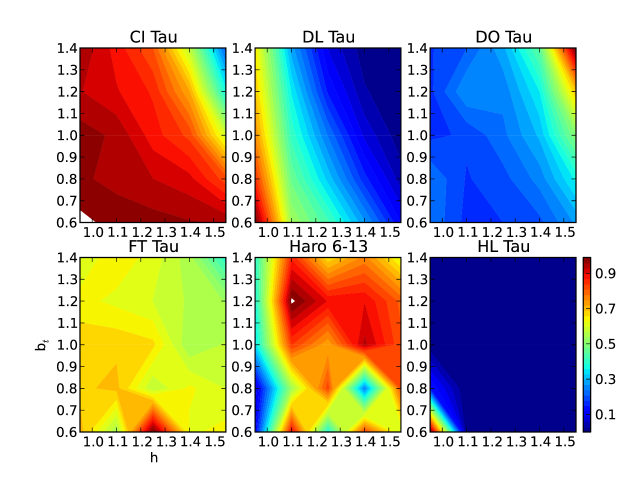
Figure 7: Disk vertical structure parameter plots. The posterior is normalized by the peak and red indicates high posterior regions.

Figure 7 shows the posterior distributions of the accretion disk models in the disk thickness (b_t) and the flareness index (h), normalized by individual peak values. As shown, the three extended disks (CI Tau, DL Tau, and HL Tau) have higher posteriors in thinner and less flared models. In contrast, DO Tau appears to be better fit by thick and more flared models. In the cases of FT Tau and Haro 6-13, distinct preferences are not present. We argue that the sensitivity and angular resolution of the data are not good enough for these objects. Note that they are the two faintest targets and compact disks of our sample.

While our modeling results of millimeter wavelength data prefer thinner and less flared disks for CI Tau, DL Tau, and HL Tau, a thick disk model can be required for shorter mid-IR observations. For example, HL Tau needs a thick disk for its mid-IR fluxes, as shown in Kwon et al. (2011). The discrepancy can be understood by stratified grain settlement: large grains, which millimeter data are sensitive to, have been settled down in the mid-plane, while fine grains are not.

The dust opacity spectral indexes $\beta$ do not have a clear (anti-)correlation with the disk thickness/flareness nor the disk sizes, while larger disks are thinner and less flared. Therefore, it may imply that large grain settlement is not the only mechanism for thinner and less-flared disks. This is consistent with the fact that protoplanetary disks are evaporated and get less flared and thinner with time.

Furlan et al. (2009) argued that protoplanetary disks with grain settlement have small $n_{13-31}$ and EW($10~{}\mu$m) values. Note that EW($10~{}\mu$m) indicates the amount of small ($<5~{}\mu$m) silicate grains and $n_{13-31}$ represents the flareness of disks by intervening of protostellar emission. Unlike their argument, we did not find a strong relationship between both properties and our flare index ($h$). Probably, the short wavelength properties of EW($10~{}\mu$m) and $n_{13-31}$ are sensitive to the warm inner and/or surface disk region and relatively small grains, while our millimeter data are sensitive to the cold outer and/or deep disk region and large grains. Also, inclinations of objects may be an effective parameter, as the light path so the optical depth along line-of-sight depends on it. In contrast, we obtained a strong correlation between $s$ and EW($10~{}\mu$m) and a strong anti-correlation between $\beta$ and $n_{13-31}$.

5.7 Disk Substructures

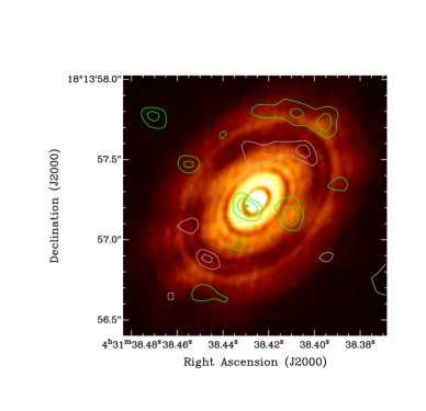
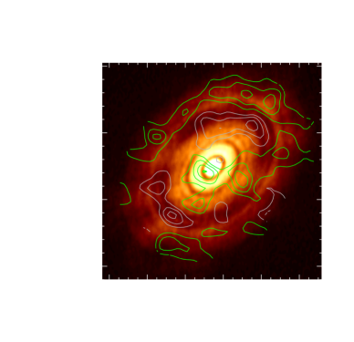
Figure 8: ALMA SV data of HL Tau in Band 7 (343.5 GHz) with an angular resolution of $0.03^{\prime\prime}\times 0.02^{\prime\prime}$ ($-176\arcdeg$) in color scales, overlaid with the residuals of our CARMA data at $\lambda=1.3$ mm after subtraction of the disk model in contours. The green and gray contours indicate positive and negative levels of 2, 3, and 4 times 0.75 mJy beam^-1, respectively. The image in the right has an additional contour of 0.75 mJy beam^-1 and the region out of the disk less than 3 mJy beam^-1 has been masked. The coordinates are in epoch of 2014 Oct. 31, when the ALMA data were taken, and our CARMA data were shifted by the proper motion. Note that the residuals nicely match the gaps and rings.

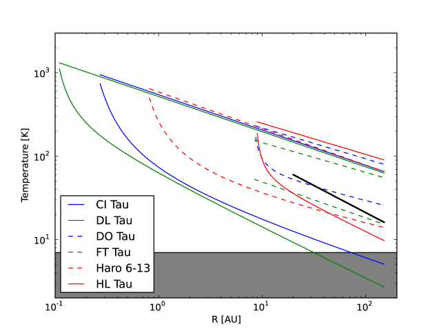
Figure 9: Comparisons of temperature distributions particularly for HL Tau in ALMA SV data and our modeling. Radial distributions of surface ($T_{s}$, upper straight lines) and mid-plane ($T_{m}$, lower curves) temperatures are shown for each of the best fitting accretion disk models. The black straight line indicates the power-law temperature distribution outlining the brightness temperature distribution of the ALMA SV data (Partnership et al., 2015): $T_{B}\textrm{[K]}=60(R/20\textrm{AU})^{-0.65}$. The lower limit of dust temperatures in our modeling is 7 K.

As discussed in Kwon et al. (2011), HL Tau has a region between 50 and 100 AU, which is gravitationally unstable and could fragment. The prediction of substructures in HL Tau has been proved by the ALMA SV data with the unprecedented angular resolution up to $0.02^{\prime\prime}$, which resolves at least 8 gaps (and rings). Particularly, the data present a wide gap between 50 and 100 AU. Indeed, our CARMA data show a hint of the wide ring, as shown in Figure 8. In addition, the positive and negative residuals nicely line up with the rings and gaps. For the comparison of the CARMA residuals with the ALMA image, we shifted CARMA data by the proper motion. The HL Tau center positions are (R.A., Dec. in J2000) = (04:31:38.418, +18:13:57.37) in the CARMA observations on 2009 Jan. 31 and (04:31:38.42545, +18:13:57.242) in the ALMA observations on 2014 Oct. 30 (Partnership et al., 2015), so the proper motion is estimated as $v_{R.A.}=18$ mas year^-1 and $v_{decl.}=-22$ mas year^-1 during the 5.75 year span. In addition, the temperature distributions of our modeling are consistent with the brightness temperature estimated by the ALMA multi-band SV data. Figure 9 shows examples of our model temperature distributions in color solid and dashed lines. In each case, the upper straight line is for the surface temperature and the bottom curve or line is for the mid-plane temperature. As described in Section 4, the temperatures were obtained by fitting RADMC 3D results. The black line is the outline of the brightness temperature estimated from the ALMA multi-band SV data (Figure 3.d of Partnership et al., 2015). Note that the brightness temperature is between the surface and mid-plane temperatures of our modeling, which means that our temperature distributions are reasonable.

Like HL Tau, whose CARMA data show a hint and whose ALMA data provide the detailed substructures, CI Tau and DL Tau images also show a possible non-axisymmetric feature. We calculated the Toomre Q parameter to check if the three extended targets have gravitationally unstable regions. The Q parameter is defined as (Toomre, 1964),

$$Q\equiv\frac{c_{s}\Omega}{\pi G\Sigma},$$ (13)

where $c_{s}$ is the isothermal sound speed, $\Omega$ is the orbital angular velocity ($\Omega=\sqrt{GM_{*}/R^{3}}$), $G$ is the gravitational constant, and $\Sigma$ is the surface density, and regions of $Q\lesssim 1.5$ are gravitationally unstable. As we constrained disk temperature and density distributions, the $Q$ parameter can be calculated assuming Keplerian rotation. Note that we utilize our mid-plane temperature distributions for $c_{s}$, instead of a constant temperature: $c_{s}^{2}=kT_{m}^{2}$.

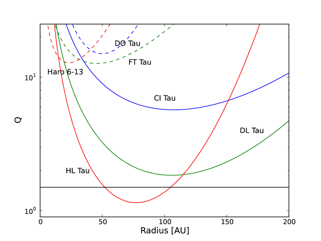
Figure 10: The Toomre $Q$ parameter along radius in the accretion disk model.

Figure 10 shows the $Q$ parameter along radius in the accretion disk models. As shown in the figure, CI Tau and DL Tau have the smallest $Q$ minima with HL Tau, but they do not have a region with $Q<1.5$. However, it is possible that they could have undetectable mass in large grains, as discussed for the correlation between $\beta$ and disk mass in Section 5.5: in particular, $\beta$ of CI Tau is close to 0. On the other hand, DL Tau has a region with the $Q$ values very close to 1.5 around 100 AU in radius, although the sensitivity of our data does not provide any distinct non-axisymmetric features.

Non-axisymmetric substructures are a possible place for protoplanet formation developed by gravitational instability. Also, they allow us to study the accretion mechanism at the late stage of star formation. A trailing spiral structure built by gravitational instability is an efficient mechanism to transport angular momentum outward (e.g., Hartmann, 2001). Therefore, if we could obtain the kinematics of such a feature along, we can study the accretion mechanism. As the SV data proved, high angular resolution and sensitivity observations of ALMA will clearly show whether or not the extended disks of our sample have a substructure and enable us to study the accretion mechanism.

While the accretion mechanism of the gravitational instability generally appears in the outer disk region, the most successful mechanism to explain angular momentum transport in the accretion disks is the magnetorotational instability (MRI) (e.g., Balbus, 2003). The key aspects MRI requires are magnetic fields coupled with material to act as a tension and disk rotational velocities decreasing outward. As with the trailing spiral arms, in which the gravity of the mass excess acts as a tension, a faster rotating inner region is dragged by the slower rotating outer region connected by the magnetic field tension. Therefore, angular momentum is transported outward. The rotation decreasing outward is a general property of circumstellar disks, whose velocity appears Keplerian. For the former aspect of magnetic fields coupled with disk material, the key property of disks is ionization fraction. Gammie (1996) tackled which parts of disks are coupled with magnetic fields and suggested a layered accretion disk. While the inner region ($<0.1$ AU) is collisionally ionized, the outer region is layered with accretionally active (ionized enough by cosmic rays) and dead zones (cold mid-plane).

The viscous accretion disk model provides a means to investigate the physical origin of viscosity. Viscosity of disks is normally parameterized as $\nu=\alpha c_{s}H$, where $\alpha$ is a dimensionless parameter, $c_{s}$ is a sound speed, and $H$ is a scale height (e.g., Shakura & Sunyaev, 1973). On the other hand, since the mass accretion rate is related to the viscosity in a structure-determined disk (e.g., Equation A10 in Andrews et al., 2009), we can estimate the $\alpha$ parameter of our disk models fitting data, assuming an accretion rate. For this calculation, we use the mass accretion rate estimated by Robitaille et al. (2007) using SED fitting (Table 7) and the equation derived by Andrews et al. (2009):

$$\alpha\approx\frac{2R_{c}^{2}}{3(2-\gamma)}\frac{\dot{M}_{*}}{M_{d}}\Big{(}\frac{R}{R_{c}}\Big{)}^{\gamma}\frac{1}{c_{s}H}.$$ (14)

Although the accretion rates determined by UV and optical spectroscopy are more accurate (Robitaille et al., 2007), we adopted the SED fitting results in order to have as many target values as possible. Note that the values estimated by UV and optical spectroscopy are available for CI Tau, DL Tau and DO Tau and are close to the minima of the SED fitting results in the parentheses of Table 7. The $\alpha$ is a function of radius but we listed only the values at 10 AU and 100 AU. The $\alpha$ values at 10 and 100 AU of our sample disks are all in the range that MRI can be the viscosity origin for: 0.005–0.6 (Balbus, 2003). We assumed the accretion rate of Haro 6-13, which has not been reported, as a typical value of $1.0\times 10^{-7}~{}\textrm{M}_{\sun}~{}\textrm{year}^{-1}$. The investigation of the viscosity origin is beyond the scope of this study, so further attempts to understand the exception are not made.

6 Conclusion

We have carried out a T Tauri disk survey using CARMA, which provides excellent image fidelity and angular resolution. We have acquired multi-wavelength ($\lambda=1.3$ mm and 2.7 mm) and multi-configuration (A, B, C, and/or D) data up to angular resolution of $0.13^{\prime\prime}$ toward 6 targets: CI Tau, DL Tau, DO Tau, FT Tau, Haro 6-13, and HL Tau. Using visibility modeling with Bayesian inference, we obtained disk properties of the flared viscous accretion disk model such as density distribution, dust opacity spectral index, disk mass, disk inner and characteristic radii, inclination, position angle, and disk vertical structures. In addition, we examined anti/correlations between the properties. The power-law disk model was also employed for investigating which disk model is preferred.

1. We found that the accretion disk model is preferred overall, with the exception of DL Tau, which prefers the power-law disk model. However, the understanding of the discrepancy is not clear at the moment. ALMA observations with a better sensitivity and angular resolution toward a large number of protoplanetary disks are required for such model comparison and trend investigation further.

2. We obtained correlations between the properties we constrained using the flared accretion disk model. Particularly, we found that disks with a steeper mid-plane density gradient have smaller $\beta$ (large grains) and are less massive. This suggests that grains grow and radially move and implies that a less massive disk has a larger fraction of large grains. In addition, we found that extended disks tend to be less flared.

3. We detected a non-axisymmetric feature toward CI Tau with a similar pattern at both millimeter wavelengths. However, the Toomre Q parameter criterion does not support a gravitationally unstable structure in CI Tau. It is interesting to note that its $\beta$ is close to 0, which implies that the mass might be underestimated. On the other hand, as discussed in previous studies (e.g., Kwon et al., 2011), HL Tau has a gravitationally unstable region between 50 and 100 AU, where we marginally detected a possible substructure and the ALMA SV data present a wide gap. Also, DL Tau has a region around 100 AU with the Q values very close to the gravitational instability regime. ALMA observations toward these objects will provide a more clear view.

Figure 2: uv amplitude plots of targets with their best fitting models for the accretion disk model in solid lines and the power-law disk model in dashed lines. $\beta$ values are calculated from the observational data simply assuming optically thin and Rayleigh-Jeans approximations. The $\beta$ results without these approximations are shown in the modeling. Open squares and triangles are for $\lambda=1.3$ mm and $\lambda=2.7$ mm data, respectively.

Figure 5: Disk continuum, model, and residual maps at $\lambda=1.3$ mm and 2.7 mm for the accretion disk models. From the left, individual target observational images, best models, and residual maps, and the upper and lower panels are at $\lambda=1.3$ mm and 2.7 mm, respectively. Note that the $\lambda=1.3$ mm images are the same as the color images of Figure 1. The images are re-centered by the phase-center offsets listed in Table 3, and the contour levels are $\pm$ 2.5, 4.0, 6.3, 10, 16, 25, 40, and 100 times individual target $\sigma$ listed in Table 3. The synthesized beams are marked in the bottom right corner of the observational images.

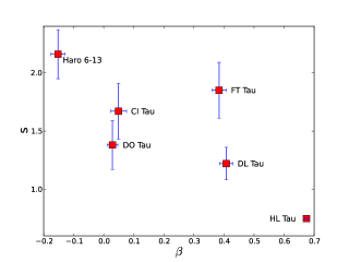
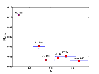
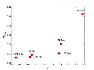
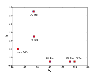
Figure 6: Relationship between properties: the mid-plane density gradient $s$ vs. $\beta$, $M_{disk}$ vs. $s$, the flare index $h$ vs. $R_{c}$, and $M_{disk}$ vs. $\beta$ from the upper left clockwise.

Table 1: Reference positions and stellar parameters

Targets	Positions (J2000)		Teff	L∗	M∗	EW(10$\mu$m)	$n_{13-31}$
	h m s	$\arcdeg~{}^{\prime}~{}^{\prime\prime}$	[K]	[L$\sun$]	[M$\sun$]
CI Tau	04 33 52.000	+22 50 30.20	4060	1.40	0.70	2.55	-0.17
DL Tau	04 33 39.076	+25 20 38.14	4060	1.12	0.70	0.51	-0.77
DO Tau	04 38 28.583	+26 10 49.85	3850	2.70	0.70	0.94	-0.13
FT Tau	04 23 39.178	+24 56 14.30	3890	0.38	0.70	1.86	-0.46
Haro 6-13	04 32 15.410	+24 28 59.97	3850	2.11	0.55	3.87	0.38
HL Tau	04 31 38.471	+18 13 58.11	4000	8.30	0.55	–	–
.

Table 2: Protoplanetary disk observations

Targets	Obs. Dates	Array	Wavelengths	Flux cal.	Gain cal..
CI Tau	2007 Nov. 25	B	1	MWC349 (1.9)	0530+135 (2.4), 3C84 (4.2)
CI Tau	2007 Sep. 18	C	1	Mars	0530+135 (3.0)
CI Tau	2008 Jun. 13	D	1	Uranus	0530+135 (1.6), 3C111 (1.7)
CI Tau	2008 Jan. 18	B	3	MWC349 (1.3)	0530+135 (3.8), 3C84 (7.1)
CI Tau	2008 Oct. 29	C	3	3C273 (14)	0530+135 (2.0)
CI Tau	2009 Mar. 30	D	3	Uranus	0510+180 (1.1), 3C111 (2.8)
DL Tau	2008 Dec. 11	B	1	3C84 (5.0)	0510+180 (0.9)
DL Tau	2008 Dec. 14	B	1	3C84 (5.0)	0510+180 (0.9)
DL Tau	2009 Mar. 11	D	1	Uranus	0510+180 (0.9), 3C111 (2.3)
DL Tau	2009 Jan. 21	A	3	3C454.3 (10)	0510+180 (1.3), 3C111 (3.8)
DL Tau	2009 Jan. 22	A	3	3C84 (9.0)	0510+180 (1.3)
DL Tau	2008 Oct. 21	C	3	Uranus	0530+135 (2.0), 3C111 (6.9)
DL Tau	2008 Oct. 29	C	3	Uranus	0530+135 (2.0), 3C111 (6.9)
DO Tau	2007 Nov. 27	B	1	MWC349 (1.9)	0510+180 (0.6)
DO Tau	2009 Nov. 4	C	1	Uranus	3C111 (1.2), 0510+180 (0.5)
DO Tau	2009 Mar. 27	D	1	Uranus	0510+180 (0.8), 3C111 (2.0)
DO Tau	2008 Oct. 18	C	3	3C84 (9.0)	0530+135 (2.0)
DO Tau	2008 Oct. 28	C	3	Uranus	0530+135 (2.0), 3C111 (6.9)
DO Tau	2008 Oct. 28	C	3	3C84 (9.0)	0530+135 (2.0)
FT Tau	2011 Jan. 5	B	1	Uranus	3C111 (3.2), 0336+323 (0.9)
FT Tau	2008 Oct. 15	C	1	Uranus	0357+233 (0.35)
FT Tau	2009 Feb. 15	A	3	Uranus	0510+180 (1.3), 3C111 (3.5)
FT Tau	2008 Oct. 26	C	3	3C454.3 (20)	0530+135 (2.0), 3C111 (6.9)
Haro 6-13	2008 Jan. 12	B	1	3C454.3 (11)	0530+135 (2.2)
Haro 6-13	2008 Apr. 25	C	1	Uranus	0530+135 (2.0), 3C111 (1.9)
Haro 6-13	2010 Jan. 29	A	3	Uranus	3C111 (2.4), 0336+323 (2.1)
Haro 6-13	2009 Jan. 4	B	3	Uranus	0510+180 (1.3)
Haro 6-13	2009 Apr. 18	C	3	Uranus	0510+180 (1.0), 3C111 (2.6)
HL Tau	2009 Jan. 17	A	1		0510+180 (0.9)
HL Tau	2009 Jan. 31	A	1	3C84	0510+180 (0.9)
HL Tau	2009 Jan. 1	B	1	3C84 (5.0)	0510+180 (0.9)
HL Tau	2007 Nov. 4	C	1	Uranus	0530+135 (2.6)
HL Tau	2008 Feb. 16	B	3	Uranus	0530+135 (4.0), 3C111 (6.7)
HL Tau	2008 Oct. 27	C	3	Uranus	0530+135 (2.0)

Table 3: Reduced data sets. The total fluxes are estimated as a flux sum over the target region beyond 2$\sigma$ levels and their uncertainties are statistical, which do not include the absolute flux calibration uncertainties. The $\Delta$RA and $\Delta$Dec are offsets of target positions from the phase centers.

Targets	Arrays	Freq.	uv coverage		Beam	RMS	Total flux		Gaussian fit sizes	$\Delta$RA	$\Delta$Dec
		[GHz]	[k$\lambda$]		[${}^{\prime\prime}\times^{\prime\prime}$ (PA°)]	[mJy beam-1]	[mJy]		[${}^{\prime\prime}\times^{\prime\prime}$ (PA°)]	[′′]	[′′]
CI Tau	BCD	229	6.8—	726.5	$0.45\times 0.31$ (-81)	1.8	97.8 $\pm$	5.7	$0.82\times 0.64$ (-14)	0.24	-0.20
	BCD	113	3.9—	363.8	$0.95\times 0.69$ (89)	0.55	28.3 $\pm$	1.5	$1.04\times 0.92$ (13)
DL Tau	BD	229	8.5—	723.8	$0.49\times 0.29$ (82)	0.97	194.2 $\pm$	4.8	$1.02\times 0.78$ (59)	0.05	-0.26
	AC	113	7.4—	727.6	$0.31\times 0.27$ (-83)	0.57	35.0 $\pm$	2.4	$1.14\times 1.11$ (9)
DO Tau	BCD	229	7.0—	616.6	$0.48\times 0.42$ (80)	1.2	125.4 $\pm$	3.5	$0.59\times 0.47$ (89)	0.07	-0.58
	C	113	8.3—	143.8	$1.75\times 1.19$ (83)	0.67	30.8 $\pm$	1.3	point source
FT Tau	BC	229	17.0—	620.0	$0.44\times 0.29$ (-71)	1.1	104.1 $\pm$	3.3	$0.46\times 0.37$ (-52)	0.20	-0.30
	AC	113	4.1—	727.6	$0.31\times 0.28$ (-9)	0.53	28.8 $\pm$	2.0	$1.27\times 0.85$ (72)
Haro 6-13	BC	229	12.3—	616.6	$0.54\times 0.39$ (-54)	2.3	111.2 $\pm$	4.9	$0.34\times 0.28$ (-7)	0.15	-0.59
	ABC	113	8.0—	727.6	$0.34\times 0.29$ (-84)	0.48	28.7 $\pm$	1.0	$0.26\times 0.20$ (-69)
HL Tau	ABC	229	15.5—	1452.0	$0.17\times 0.13$ (85)	0.75	685.0 $\pm$	6.7	$0.85\times 0.64$ (-46)	-0.75	-0.74
	BC	112	8.0—	359.0	$1.01\times 0.67$ (73)	0.93	118.4 $\pm$	2.6	$0.84\times 0.71$ (-23)

Table 4: Disk fitting results of free parameters.

Viscous accretion disk model
Targets	$s$	$\beta$	$M_{disk}$	$R_{in}$	$R_{c}$	$\theta_{i}$	PA	$\gamma$	$R_{t}$
			[M⊙]	[AU]	[AU]	[$\arcdeg$]	[$\arcdeg$]		[AU]
CI Tau	1.67$\pm$0.24	0.049$\pm$0.027	0.018$\pm$0.002	4.2$\pm$2.6	119.6$\pm$6.1	61.0$\pm$2.9	17.6$\pm$2.6	(0.72)	(57.4)
DL Tau	1.22$\pm$0.14	0.408$\pm$0.022	0.041$\pm$0.005	1.3$\pm$1.1	112.2$\pm$2.4	-38.6$\pm$1.3	55.2$\pm$2.0	(0.27)	(54.8)
DO Tau	1.38$\pm$0.21	0.029$\pm$0.018	0.014$\pm$0.001	6.7$\pm$1.6	54.2$\pm$1.1	-32.5$\pm$2.0	89.7$\pm$3.8	(-0.17)	(27.6)
FT Tau	1.85$\pm$0.24	0.384$\pm$0.024	0.021$\pm$0.002	8.09$\pm$0.98	55.2$\pm$2.0	33.8$\pm$1.7	136.1$\pm$2.9	(0.60)	(26.5)
Haro 6-13	2.16$\pm$0.21	-0.152$\pm$0.024	0.012$\pm$0.001	1.6$\pm$1.3	28.9$\pm$2.1	41.5$\pm$3.3	167.2$\pm$5.8	(1.06)	(14.8)
HL Tau	0.7483$\pm$0.0087	0.6745$\pm$0.0069	0.105$\pm$0.001	8.78$\pm$0.19	80.20$\pm$0.34	41.19$\pm$0.22	135.38$\pm$0.34	(-0.20)	(40.9)
Power-law disk model
Targets	$s$	$\beta$	$M_{disk}$	$R_{in}$	$R_{out}$	$\theta_{i}$	PA	$p$
			[M⊙]	[AU]	[AU]	[$\arcdeg$]	[$\arcdeg$]
CI Tau	2.15$\pm$0.25	0.036$\pm$0.027	0.017$\pm$0.002	6.5$\pm$2.0	195$\pm$11	62.5$\pm$2.6	17.7$\pm$2.5	(1.05)
DL Tau	2.08$\pm$0.23	0.387$\pm$0.021	0.029$\pm$0.003	8.18$\pm$0.89	152.6$\pm$2.3	-38.4$\pm$1.3	55.6$\pm$2.0	(0.53)
DO Tau	1.98$\pm$0.23	0.021$\pm$0.018	0.013$\pm$0.001	7.3$\pm$1.5	75.4$\pm$2.0	-32.8$\pm$2.0	90.7$\pm$3.5	(0.43)
FT Tau	2.80$\pm$0.15	0.341$\pm$0.024	0.015$\pm$0.002	8.70$\pm$0.27	98.2$\pm$5.1	33.2$\pm$1.7	136.0$\pm$3.0	(1.25)
Haro 6-13	2.76$\pm$0.21	-0.164$\pm$0.024	0.011$\pm$0.002	1.54$\pm$0.65	61.9$\pm$5.2	43.5$\pm$2.9	167.3$\pm$5.9	(1.81)
HL Tau	2.14$\pm$0.01	0.615$\pm$0.006	0.067$\pm$0.001	8.70$\pm$0.02	109.71$\pm$0.23	40.9$\pm$0.20	135.7$\pm$0.34	(0.59)

Table 5: Disk model comparison.

Targets	ln($P(D\mid H_{A})$)	ln($P(D\mid H_{P})$)	ln($K$)	Preferable model
CI Tau	-1221129.9	-1221128.1	0.8	Comparable
DL Tau	-5336360.9	-5336365.6	-4.7	Power-law
DO Tau	-1794530.0	-1794521.3	8.7	Accretion
FT Tau	-5444060.7	-5444044.3	16.4	Accretion
Haro 6-13	-3053420.6	-3053420.1	0.5	Comparable
HL Tau	-7863636.4	-7863346.8	289.6	Accretion

Table 6: Correlation coefficients between properties. HL Tau is not included in the relationships with EW($10~{}\mu$m) and $n_{13-31}$ and the bold-font anti/correlations are plotted in Figure 6.

Properties	$\beta$	$M_{disk}$	$R_{in}$	$R_{c}$	$h$	EW	$n_{13-31}$
$s$	-0.77	-0.84	-0.41	-0.47	0.21	0.93	0.74
$\beta$	1.00	0.84	0.52	0.36	-0.36	-0.70	-0.95
$M_{disk}$		1.00	0.44	0.26	-0.48	-0.65	-0.86
$R_{in}$			1.00	-0.16	0.34	-0.23	-0.13
$R_{c}$				1.00	-0.59	-0.44	-0.63
$h$					1.00	-0.25	0.19
EW($10~{}\mu$m)						1.00	0.83
$n_{13-31}$							1.00

Table 7: Disk mass accretion properties.

Targets	$\dot{M}_{disk}$	$M_{disk}\tablenotemark{b}/\dot{M}_{disk}$	$\alpha$(10 AU)	$\alpha$(100 AU)
	[$\times 10^{-7}$ M⊙ year-1]	[$\times 10^{5}$ year]
CI Tau	1.2 (0.49–2.6)	1.5	0.43	0.18
DL Tau	1.2 (0.69–1.2)	3.5	0.30	0.098
DO Tau	6.8 (1.5–6.8)	0.2	0.37	0.017
FT Tau	0.51 (0.028–1.6)	4.0	0.029	0.014
Haro 6-13	1.0	1.2	0.018	0.013
HL Tau	10 (3.0–51)	1.0	0.41	0.079

References

- Andrews & Williams (2005) Andrews, S. M., & Williams, J. P. 2005, ApJ, 631, 1134
- Andrews & Williams (2007) —. 2007, ApJ, 659, 705
- Andrews et al. (2009) Andrews, S. M., Wilner, D. J., Hughes, A. M., Qi, C., & Dullemond, C. P. 2009, ApJ, 700, 1502
- Ayliffe & Bate (2009) Ayliffe, B. A., & Bate, M. R. 2009, MNRAS, 397, 657
- Balbus (2003) Balbus, S. A. 2003, ARA&A, 41, 555
- Beckwith & Sargent (1991) Beckwith, S. V. W., & Sargent, A. I. 1991, ApJ, 381, 250
- Beckwith et al. (1990) Beckwith, S. V. W., Sargent, A. I., Chini, R. S., & Guesten, R. 1990, AJ, 99, 924
- Bertout et al. (1999) Bertout, C., Robichon, N., & Arenou, F. 1999, A&A, 352, 574
- Briggs (1995) Briggs, D. S. 1995, PhD thesis, New Mexico Institute of Mining and Technology
- Carpenter et al. (2014) Carpenter, J. M., Ricci, L., & Isella, A. 2014, ApJ, 787, 42
- Draine (2006) Draine, B. T. 2006, ApJ, 636, 1114
- Dullemond & Dominik (2004) Dullemond, C. P., & Dominik, C. 2004, A&A, 417, 159
- Furlan et al. (2009) Furlan, E., Watson, D. M., McClure, M. K., et al. 2009, ApJ, 703, 1964
- Gammie (1996) Gammie, C. F. 1996, ApJ, 457, 355
- Gilks et al. (1996) Gilks, W. R., Richardson, S., & Spiegelharlter, D. J. 1996, Markov Chain Monte Carlo in Practice (Chapman and Hall)
- Guilloteau et al. (2011) Guilloteau, S., Dutrey, A., Piétu, V., & Boehler, Y. 2011, A&A, 529, A105
- Hartmann (2001) Hartmann, L. 2001, Accretion Processes in Star Formation, ed. L. Hartmann
- Hartmann et al. (1998) Hartmann, L., Calvet, N., Gullbring, E., & D’Alessio, P. 1998, ApJ, 495, 385
- Hildebrand (1983) Hildebrand, R. H. 1983, QJRAS, 24, 267
- Hughes et al. (2008) Hughes, A. M., Wilner, D. J., Qi, C., & Hogerheijde, M. R. 2008, ApJ, 678, 1119
- Isella et al. (2009) Isella, A., Carpenter, J. M., & Sargent, A. I. 2009, ApJ, 701, 260
- Isella et al. (2010) —. 2010, ApJ, 714, 1746
- Kass & Raftery (1995) Kass, R. E., & Raftery, A. E. 1995, Journal of the American Statistical Association, 90, 773
- Kenyon et al. (1994) Kenyon, S. J., Dobrzycka, D., & Hartmann, L. 1994, AJ, 108, 1872
- Kenyon & Hartmann (1995) Kenyon, S. J., & Hartmann, L. 1995, ApJS, 101, 117
- Kitamura et al. (2002) Kitamura, Y., Momose, M., Yokogawa, S., et al. 2002, ApJ, 581, 357
- Koerner & Sargent (1995) Koerner, D. W., & Sargent, A. I. 1995, AJ, 109, 2138
- Kwon (2009) Kwon, W. 2009, PhD thesis, University of Illinois at Urbana-Champaign
- Kwon et al. (2011) Kwon, W., Looney, L. W., & Mundy, L. G. 2011, ApJ, 741, 3
- Kwon et al. (2009) Kwon, W., Looney, L. W., Mundy, L. G., Chiang, H., & Kemball, A. J. 2009, ApJ, 696, 841
- Lamb et al. (2009) Lamb, J., Woody, D., Bock, D., et al. 2009, in SPIE Newsroom
- Lay et al. (1997) Lay, O. P., Carlstrom, J. E., & Hills, R. E. 1997, ApJ, 489, 917
- MacKay (2003) MacKay, D. J. C. 2003, Information Theory, Inference, and Learning Algorithms (Cambridge, UK: Cambridge University Press)
- Mathis et al. (1977) Mathis, J. S., Rumpl, W., & Nordsieck, K. H. 1977, ApJ, 217, 425
- McCuskey (1938) McCuskey, S. W. 1938, ApJ, 88, 209
- Mundy et al. (1996) Mundy, L. G., Looney, L. W., Erickson, W., et al. 1996, ApJ, 464, L169+
- Ossenkopf & Henning (1994) Ossenkopf, V., & Henning, T. 1994, A&A, 291, 943
- Partnership et al. (2015) Partnership, A., Brogan, C. L., Perez, L. M., et al. 2015, ArXiv e-prints
- Pérez et al. (2012) Pérez, L. M., Carpenter, J. M., Chandler, C. J., et al. 2012, ApJ, 760, L17
- Preibisch & Smith (1997) Preibisch, T., & Smith, M. D. 1997, A&A, 322, 825
- Press et al. (1996) Press, W. H., Teukolsky, S. A., Vetterling, W. T., & Flannery, B. F. 1996, Numerical Recipes in Fortran 77 (2nd ed. New York : the Press Syndicate of the University of Cambridge. ISBN : 052143064X)
- Pringle (1981) Pringle, J. E. 1981, ARA&A, 19, 137
- Rebull et al. (2004) Rebull, L. M., Wolff, S. C., & Strom, S. E. 2004, AJ, 127, 1029
- Robitaille et al. (2007) Robitaille, T. P., Whitney, B. A., Indebetouw, R., & Wood, K. 2007, ApJS, 169, 328
- Sandell et al. (2011) Sandell, G., Weintraub, D. A., & Hamidouche, M. 2011, ApJ, 727, 26
- Sault et al. (1995) Sault, R. J., Teuben, P. J., & Wright, M. C. H. 1995, in Astronomical Society of the Pacific Conference Series, Vol. 77, Astronomical Data Analysis Software and Systems IV, ed. R. A. Shaw, H. E. Payne, & J. J. E. Hayes, 433–+
- Schaefer et al. (2009) Schaefer, G. H., Dutrey, A., Guilloteau, S., Simon, M., & White, R. J. 2009, ApJ, 701, 698
- Shakura & Sunyaev (1973) Shakura, N. I., & Sunyaev, R. A. 1973, A&A, 24, 337
- Simon et al. (2000) Simon, M., Dutrey, A., & Guilloteau, S. 2000, ApJ, 545, 1034
- Smith et al. (1999) Smith, K. W., Lewis, G. F., Bonnell, I. A., Bunclark, P. S., & Emerson, J. P. 1999, MNRAS, 304, 367
- Thompson et al. (2001) Thompson, A. R., Moran, J. M., & Swenson, Jr., G. W. 2001, Interferometry and Synthesis in Radio Astronomy, 2nd Edition (Interferometry and synthesis in radio astronomy by A. Richard Thompson, James M. Moran, and George W. Swenson, Jr. 2nd ed. New York : Wiley, c2001.xxiii, 692 p. : ill. ; 25 cm. “A Wiley-Interscience publication.” Includes bibliographical references and indexes. ISBN : 0471254924)
- Toomre (1964) Toomre, A. 1964, ApJ, 139, 1217
- Trotta et al. (2013) Trotta, F., Testi, L., Natta, A., Isella, A., & Ricci, L. 2013, Astronomy & Astrophysics, 558, A64
- van der Marel et al. (2013) van der Marel, N., van Dishoeck, E. F., Bruderer, S., et al. 2013, Science, 340, 1199
- Weidenschilling (1977) Weidenschilling, S. J. 1977, Ap&SS, 51, 153