Long-Term Stability Analysis of Power Systems with Wind Power Based on Stochastic Differential Equations: Model Development and Foundations

Abstract

In this paper, the variable wind power is incorporated into the dynamic model for long-term stability analysis. A theory-based method is proposed for power systems with wind power to conduct long-term stability analysis, which is able to provide accurate stability assessments with fast simulation speed. Particularly, the theoretical foundation for the proposed approximation approach is presented. The accuracy and efficiency of the method are illustrated by several numerical examples.

I Introduction

Steady increase in load demands and aging transmission networks have pushed many power systems closer to their stability limit [1]. Previous practical experience shows that the system may remain stable in the short-term time scale (say 0-30s after the contingency) while becomes unstable in the long-term time scale (say 30s-several minutes after the contingency) due to insufficient reactive power support or poor control schemes [2]-[7]. The focus of long-term stability is on slower and longer duration phenomena after generator dynamics damp out [4]-[6]. In this time scale, two-time scale decomposition of the power system dynamic model can be employed [2][3]. Particularly, the dynamics can be classified into short-term dynamics and long-term dynamics based on the time frames of function after contingencies. As the penetration of wind power continues to grow, the long-term stability of a system may be further affected by the volatile nature of wind power and the distinct dynamic response characteristics of wind turbines [8]. Long-term stability analysis deserves more attention to better ensure the secure operation of power grids. It is also crucial to study the impacts of wind power on long-term stability.

In previous literature, impacts of wind power on long-term stability have been discussed in [9][10], which focus on the effects of different control schemes of wind generators. Stability impacts of wind power on transient stability and small signal stability have been discussed in [11]-[15]. In all above studies, power systems are formulated in ordinary differential equations (ODEs) or differential algebraic equations (DAEs), and wind speed is assumed to be constant without considering the statistic properties of wind. To study the effects of the variability of wind power, stochastic differential equations (SDEs) are employed in [16]-[18] for transient stability and small-signal stability. In those studies, the variations induced by wind speed are simply modelled as white noise perturbations on power injections without characterizing the statistic properties of wind speed. In [19], a set-theoretic method is proposed to assess the effect of variability of renewable energies on short-term dynamics under small perturbations. Regarding long-term stability study of power systems with wind power, the challenges include the stochastic characterization of wind power and the resulting high computational burden in stability assessments, which have not been well addressed. Specifically, introduction of the randomness will clearly increase the computational burden, making the stability assessments of stochastic systems time consuming.

In this paper, the statistic properties of wind power are well characterized and incorporated in stability analysis; a method is proposed with its theoretical foundation for long-term stability analysis, which is able to reduce the computational burden arising from the randomness. Particularly, a SDE-based model [21] is utilized to characterize the Weibull-distributed wind speed, which is further incorporated into the complete dynamic model described in SDEs. Under this SDE formulation, a theory-based method, which is to approximate the stochastic model by a deterministic model, is proposed to perform long-term stability analysis. The theoretical foundation for the method is also developed under which the accuracy of the deterministic model is guaranteed. Compared to the deterministic models using constant wind speeds, the proposed deterministic model reflects the variable nature of wind power by providing correct stability assessments for the stochastic model. Compared to the stochastic model characterizing the statistic properties of wind speed, the proposed deterministic model takes much less time in time domain simulation.

The rest of the paper is organized as follows. Section II briefly reviews power system models. Section III introduces the preliminaries about the wind speed model by SDEs and singular perturbation method. Section IV presents the formulation of the long-term stability model with wind power based on SDEs. Afterwards, an analytical method with its theoretical foundation is proposed in Section V for long-term stability analysis of power systems with wind power. Several numerical examples are given in Section VI to illustrate the feasibility and efficiency of the proposed method. Conclusions and perspectives are stated in Section VII.

II Power System Models

The deterministic power system long-term stability model, i.e., complete dynamic model, for simulating system dynamic response relative to a disturbance can be described as:

$$\dot{z}_{c} = \epsilon{h}_{c}({z_{c},x,y,z_{d}})$$ (1)

$$\dot{{x}} = {f}({z_{c},x,y,z_{d}})$$ (2)

$${0} = {g}({z_{c},x,y,z_{d}})$$ (3)

$${z}_{d}(k) = {h}_{d}({z_{c},x,y,z_{d}(k-1)})$$ (4)

Equation (1) describes long-term dynamics including exponential recovery loads, turbine governors (TGs) and over excitation limiters (OXLs), and Eqn (2) describes the internal dynamics of devices such as generators, their automatic voltage regulators (AVRs), certain loads such as induction motors, and other dynamically modeled components. Equation (3) describes the electrical transmission system and the internal static behaviors of passive devices, and Eqn (4) describes long-term discrete events like load tap changers (LTCs) and shunt switchings. $h_{c}$, $f$ and $g$ are continuous functions, and vectors $z_{c}\in\mathbb{R}^{n_{z_{c}}}$, ${x}\in\mathbb{R}^{n_{x}}$ and ${y}\in\mathbb{R}^{n_{y}}$ are the corresponding long-term/slow state variables, short-term/fast state variables, and algebraic variables. $z_{d}\in\mathbb{R}^{n_{z_{d}}}$ are termed as long-term discrete variables whose transitions from $z_{d}(k-1)$ to $z_{d}(k)$ depend on system trajectories and occur at distinct times $t_{k}$ where $k=1,2,3,...N$. Besides, $1/\epsilon$ can be regarded as the maximum time constant among devices.

Load models play an important role in long-term stability analysis, and generally load dynamics appear in Eqn (3) as:

$$p = x_{p}/T_{p}+p_{t}$$ (5)

$$q = x_{q}/T_{q}+q_{t}$$ (6)

where $x_{p}$ and $x_{q}$ are internal state variables associated with generic load dynamics. They are described in Eqn (1) as:

$${\dot{x}_{p}} = -x_{p}/T_{p}+p_{s}-p_{t}$$ (7)

$${\dot{x}_{q}} = -x_{q}/T_{q}+q_{s}-q_{t}$$ (8)

where $p_{s}$ and $p_{t}$ are the static and transient real power absorptions; similar definition for $q_{s}$ and $q_{t}$. $p^{0}_{L}$ and $q^{0}_{L}$ are PQ load power from power flow solutions[4][20].

The tap-changing logic of LTC at time instant $t_{k}$ shows up in Eqn (4), and is given as follows:

$$m_{k+1}=\left\{\begin{array}[]{ll}m_{k}+\triangle{m}&\mbox{if }v>v_{0}+d\mbox{ and }m_{k}<m^{max}\\ m_{k}-\triangle{m}&\mbox{if }v<v_{0}-d\mbox{ and }m_{k}>m^{min}\\ m_{k}&\mbox{otherwise}\end{array}\right.$$ (9)

where $v$ is the controlled voltage of LTC, $v_{0}$ is the reference voltage, $d$ is half the LTC dead-band, and $m^{max}$ and $m^{min}$ are the upper and lower tap limits [2][4][20].

III Mathematical Preliminaries

In this section, the method to model the Weibull-distributed wind speed by SDE proposed in [21][22] is briefly reviewed. Singular perturbation theory for ODE [23] is also reviewed.

III-A Modelling Wind Speed by SDE

Two continuous wind speed models based on SDE have been developed in [21][22]. The developed models include but not limited to the autocorrelated Weibull distributed wind speed models. In this paper, model I in [21] is applied to formulate wind speed. Briefly speaking, memoryless transformation of Ornstein-Uhlenbeck process is used to obtain the Weibull distributed process.

First, consider the following stochastic differential equation with given initial condition $\eta(0)\sim\mathcal{N}(0,\beta^{2}/2\alpha)$:

$$\dot{\eta}=-\alpha\eta+\beta\xi$$ (10)

where $\xi(t)=\frac{dW(t)}{dt}$ is white noise process and $W(t)$ represents a standard Wiener process. The stochastic process $\eta(t)$ is an Ornstein-Uhlenbeck/Gauss-Markov process which is stationary, Gaussian and Markovian with the statistic properties $\mathrm{E}[\eta(t)]=0$, $\mathrm{Var}[\eta(t)]=\beta^{2}/2\alpha$, and autocorrelation $\mathrm{Aut}[\eta(t_{i}),\eta(t_{j})]=e^{-\alpha|t_{j}-t_{i}|}$.

Then we apply a memoryless transformation to $\eta(t)$ as follows:

$$\gamma(t)=F_{w}^{-1}(\Phi(\frac{\eta(t)}{\beta/\sqrt{(2\alpha)}}))$$ (11)

where $F_{w}$ is the Weibull cumulative distribution function:

$$F_{w}(u)=1-e^{(u/\lambda)^{k}},\quad\forall u>0$$ (12)

with the shape parameter $k>0$ and the scale parameter $\lambda>0$, and $\Phi$ is the Gaussian cumulative distribution function:

$$\Phi(\frac{u-\mathrm{E}[u]}{\sqrt{\mathrm{Var}[u]}})=\frac{1}{2}(1+\mathrm{erf}(\frac{u-\mathrm{E}[u]}{\sqrt{2\mathrm{Var}[u]}})),\quad\forall u\in\mathbb{R}$$ (13)

The resulting process $\gamma(t)$ is a Weibull distributed stochastic process with the statistic properties $\mathrm{E}[\gamma(t)]=\lambda\Gamma(1+\frac{1}{k})=\mu_{w}$, $\mathrm{Var}[\gamma(t)]=\lambda^{2}\Gamma(1+\frac{2}{k})-\mu_{w}^{2}$, and $\mathrm{Aut}[\gamma(t_{i}),\gamma(t_{j})]\approx e^{-\alpha|t_{j}-t_{i}|}$. Note that $\mathrm{E}[\gamma(t)]$, $\mathrm{Var}[\gamma(t)]$ and $\mathrm{Aut}[\gamma(t_{i}),\gamma(t_{j})]$ do not depend on the parameter $\beta$, i.e., $\beta$ in Eqn (10) does not affect the statistic properties of stochastic process $\gamma(t)$[21]. Since wind speed is autocorrelated in the range of hours, $\alpha$ depending on the decay rate of autocorrelation is usually small in the time frame of stability analysis.

Note that although we consider the Weibull-distributed wind speed model in this paper, Eqn (10)-(11) can be used to formulate other probability distributions by applying different $F_{w}$ in Eqn (11). Refer to [21] for more details.

III-B Singular Perturbation Theory for ODE

We next consider the following general singular perturbed model (slow-fast model):

$$\Sigma_{\epsilon}:\dot{z} = f(z,x)\qquad z\in\mathbb{R}^{n_{z}}$$ (14)

$$\epsilon\dot{x} = g(z,x)\qquad x\in\mathbb{R}^{n_{x}}$$

where $\epsilon$ is a small positive parameter. $z$ is a vector of slow variables while $x$ is a vector of fast variables.

The slow model is obtained by setting $\epsilon=0$ in (14):

$$\Sigma_{0}:\dot{z} = f(z,x)\qquad z\in\mathbb{R}^{n_{z}}$$ (15)

$$0 = g(z,x)\qquad x\in\mathbb{R}^{n_{x}}$$

The algebraic equation $0=g(z,x)$ constrains the slow dynamics to the constraint manifold defined by:

$$\Gamma:=\{(z,x)\in\mathbb{R}^{n_{z}}\times\mathbb{R}^{n_{x}}:g(z,x)=0\}$$ (16)

The trajectory of model (15) starting at $(z_{0},x_{0})$ is denoted by $\phi_{0}(t,z_{0},x_{0})$, and the stability region is defined as:

$$A_{0}(z_{s},x_{s}):=\{(z,x)\in\Gamma:\phi_{0}(t,z,x)\rightarrow(z_{s},x_{s})\mbox{ as }t\rightarrow\infty\}$$

The singular points of system (15) or singularity $S$ is defined as:

$$S:=\{(z,x)\in\Gamma:\mbox{ det}(\partial_{x}g)(z,x)=0\}$$ (17)

where $\partial_{x}g$ is the Jacobian matrix of g with respect to x.

Singular points can drastically influence the trajectories of the DAE system (15). Typically, the singular set $S$ is a set of maximal dimension $(n_{z}-1)$ embedded in $\Gamma$, and $\Gamma$ is separated by $S$ into open regions [28][29].

We next define the fast model, i.e., boundary layer model, associated with the singularly perturbed model. Define the fast time scale $\kappa=t/\epsilon$. In this time scale, model (14) takes the form:

$$\Pi_{\epsilon}:\frac{dz}{d\kappa} = {\epsilon}f(z,x)\qquad z\in\mathbb{R}^{n_{z}}$$ (18)

$$\frac{dx}{d\kappa} = g(z,x)\qquad\quad x\in\mathbb{R}^{n_{x}}$$

Let $\epsilon=0$, we obtain the fast model as follows:

$$\Pi_{f}:\frac{dz}{d\kappa} = 0\qquad\qquad z\in\mathbb{R}^{n_{z}}$$ (19)

$$\frac{dx}{d\kappa} = g(z,x)\qquad x\in\mathbb{R}^{n_{x}}$$

where $z$ is frozen and treated as a parameter. The constraint manifold $\Gamma$ is a set of equilibriums of models (19). For each fixed $z$, a fast dynamical model (19) is defined.

Definition 1: Stable Component of the Constraint Manifold / Uniformly Asymptotically Stable

Assuming $(z,x)\notin S$, and $x=j(z)$ is an isolated root of equation:

$$0=g(z,x)$$ (20)

then $x=j(z)$ is an equilibrium point of system (19) and is also termed as the slow manifold of system (14). If $x=j(z)$ is an asymptotically stable equilibrium point of system (19) for all $z\in Z$, then we say that the equilibrium point $j(z)$ is uniformly asymptotically stable, and the slow manifold $x=j(z)$ is a stable component of the constraint manifold $\Gamma$.

Under the following conditions, the slow model (15) provides good approximations of the singular perturbed model (14). Assume that the equilibrium point $x=j(z)$ of the fast model is uniformly asymptotically stable in $z\in Z$ and the initial condition $(z_{0},x_{0})$ is in the stability region $A_{t}(z_{0},j(z_{0}))$ of the initial fast model with $z_{0}\in Z$, then solution of singular perturbed model (14) will approach $j(z)$ in a time of order $\epsilon|\mbox{log}\epsilon|$, and the solution of model (14) remains in an $\epsilon$-neighbourhood of the slow manifold $j(z)$[23][25]. Furthermore, there exists an invariant manifold $x={j^{\star}}(z,\epsilon)=j(z)+O(\epsilon)$ for sufficiently small $\epsilon$ in $z\in Z$[23][30], and the dynamics on invariant manifold is given by:

$$\dot{z}=f({j^{\star}}(z,\epsilon),z)$$ (21)

which can be approximated by regular perturbation theory. Specifically, Eqn (21) is reduced to slow model (15) at $\epsilon=0$.

IV sde formulation of power system models

When the long-term stability model is represented in $\tau$ time scale, where $\tau=t\epsilon$, and $\prime$ refers to $\frac{d}{d\tau}$, the long-term stability model of power system can be represented as:

$${z}_{c}^{\prime} = {h}_{c}({z_{c},x,y,z_{d}})$$ (22)

$$\epsilon{x}^{\prime} = {f}({z_{c},x,y,z_{d}})$$ (23)

$${0} = {g}({z_{c},x,y,z_{d}})$$ (24)

$$z_{d}(k) = h_{d}(z_{c},x,y,z_{d}(k-1))$$ (25)

It is possible to decouple the long-term stability model into two decoupled systems (22)-(24) and (25). When discrete variables $z_{d}$ jump from $z_{d}(k-1)$ to $z_{d}(k)$, $z_{d}$ are updated first according to (25) and then system (22)-(24) works with fixed parameters $z_{d}$. In other words, the long-term stability model can be regarded as a collection of continuous DAE systems with fixed discrete parameters. In the remainder of this paper, we focus only on the continuous DAE system (22)-(24).

When incorporating wind power in the power system models, we use Eqn (10)-(11) to formulate wind speed. Assuming that there are $n_{w}$ wind sources in the system, and the wind model is described in $\tau$ time scale, we have

$$\epsilon\eta_{w}^{\prime} = -A\eta_{w}+\sigma\xi=f_{w}(\eta_{w})+\sigma\xi$$ (26)

$$y_{w} = \hat{F}_{w}^{-1}(\hat{\Phi}(\frac{\eta_{w}}{\sigma/\sqrt{2A}}))=g_{w}(\eta_{w})$$

where $\eta_{w},y_{w}\in\mathbb{R}^{n_{w}}$, $A=\mbox{diag}[\alpha_{1},\ldots,\alpha_{n_{w}}]\in\mathbb{R}^{{n_{w}}\times{n_{w}}}$ in which $\alpha_{i}$ is determined by autocorrelation property of each wind source, $\sigma$ is a small positive parameter, $\int_{0}^{t}\xi(s)ds$ is a $n_{w}$-dimensional Wiener process; $\hat{F}_{w}=[F_{w}(\eta_{w_{1}}),F_{w}(\eta_{w_{2}}),...F_{w}(\eta_{w_{n_{w}}})]^{T}$, $\hat{\Phi}=[\Phi(\eta_{w_{1}}),\Phi(\eta_{w_{2}}),...\Phi(\eta_{w_{n_{w}}})]^{T}$, and $g_{w}:\mathbb{R}^{n_{w}}\mapsto\mathbb{R}^{n_{w}}$.

Note that $\sigma$ does not affect statistic properties of $y_{w}$, which has the same reason that $\beta$ does not affect the statistic properties of $\gamma(t)$ as shown in the last paragraph of Section III-A. This property of the formulation will play an important role in the analysis of Section V.

With (22)-(24) and (26), the stochastic long-term stability model can be represented as:

$${z}_{c}^{\prime} = \bar{h}_{c}({z_{c},x,\bar{y},z_{d}})$$ (27)

$$\epsilon{\bar{x}}^{\prime} = \bar{f}({z_{c},\bar{x},\bar{y},z_{d}})+\sigma B{\xi}$$

$${0} = \bar{g}({z_{c},\bar{x},\bar{y},z_{d}})$$

where $\bar{x}=[x^{T},\eta_{w}^{T}]^{T}\in\mathbb{R}^{n_{x}+n_{w}}=\mathbb{R}^{n_{\bar{x}}}$, $\bar{y}=[y^{T},y_{w}^{T}]^{T}\in\mathbb{R}^{n_{y}+n_{w}}=\mathbb{R}^{n_{\bar{y}}}$, $B=\left[\begin{smallmatrix}0\\ I_{n_{w}}\end{smallmatrix}\right]$.

Under the following assumption, the stochastic DAE system (27) can be simplified as a stochastic ODE system.

Assumption 1. The trajectory of the deterministic long-term stability model (28) doesn’t meet singularity.

$${z}_{c}^{\prime} = \bar{h}_{c}({z_{c},x,\bar{y},z_{d}})$$ (28)

$$\epsilon{\bar{x}}^{\prime} = \bar{f}({z_{c},\bar{x},\bar{y},z_{d}})$$

$${0} = \bar{g}({z_{c},\bar{x},\bar{y},z_{d}})$$

Under Assumption 1, $\bar{y}$ can be expressed by $(z_{c},\bar{x},z_{d})$ from the algebraic equation as $\bar{y}=l(z_{c},\bar{x},z_{d})$. Substituting the expression back to model (27), we have:

$$z_{c}^{\prime} = H_{c}(z_{c},\bar{x},z_{d})$$ (29)

$$\epsilon\bar{x}^{\prime} = F(z_{c},\bar{x},z_{d})+\sigma B{\xi}$$

or written in the form:

$$dz_{c} = H_{c}(z_{c},\bar{x},z_{d})d\tau$$ (30)

$$d\bar{x} = \frac{1}{\epsilon}F(z_{c},\bar{x},z_{d})d\tau+\frac{\sigma}{\sqrt{\epsilon}}BdW$$

Besides, system (28) can be written as:

$$dz_{c} = H_{c}(z_{c},\bar{x},z_{d})d\tau$$ (31)

$$d\bar{x} = \frac{1}{\epsilon}F(z_{c},\bar{x},z_{d})d\tau$$

In the next section, we will provide a theoretical foundation for approximating (30) by (31) in long-term stability analysis. The deterministic model (31) can provide correct stability analysis results for the stochastic model (30) provided some mild conditions are satisfied. Compared to the stochastic model (30), the deterministic model (31) takes less time in time domain simulation. Compared to other deterministic models using constant wind speed, the deterministic model (31) reflects the variability of the wind speed by providing accurate stability assessments for (30).

V theoretical basis

In this section, we apply the singular perturbation theory for SDEs proposed in [24]-[26], to develop the theoretical foundation for approximating (30) by (31). The main results of [24]-[26] are briefly reviewed in Appendix A. Note that we have formulated the stochastic long-term stability model (30) into the conventional form (36) considered in singular perturbation theory for SDE. Specifically, $Q=0$. We further assume the counter-part of Assumption 2.1 (see Appendix A) in this specific formulation is satisfied. Note that differentiability and uniform boundedness are usually satisfied in real physical systems, and the assumption is reasonable.

We denote the slow manifold of system (31) as $\bar{x}=l_{1}(z_{c},z_{d})$. If $\bar{x}=l_{1}(z_{c},z_{d})$ is a stable component of the constraint manifold when $z_{c}\in D_{z_{c}}\subset\mathbb{R}^{z_{c}}$, then there exists an invariant manifold of system (31) that $\bar{x}=l_{1}^{\star}(z_{c},z_{d},\epsilon)=l_{1}(z_{c},z_{d})+O(\epsilon)$. We further define the ellipsoidal layer $N(h)$ surrounding the invariant manifold as below:

$$N(h) = \{(z_{c},\bar{x},z_{d}):\langle(\bar{x}-l_{1}^{\star}(z_{c},z_{d},\epsilon)),$$ (32)

$$L_{1}^{\star}(z_{c},z_{d},\epsilon)^{-1}(\bar{x}-l_{1}^{\star}(z_{c},z_{d},\epsilon))\rangle<h^{2}\}$$

where $\langle\rangle$ denotes the operator of inner product. Note that the matrix $L_{1}^{\star}(z_{c},z_{d},\epsilon)$ describing the cross section of $N(h)$ is well defined as shown in Appendix B. In addition, an illustration of $N(h)$ is shown in Fig. 1.

Figure 1: Illustration of $N(h)$ in which case $n_{z}=1$, $n_{\bar{x}}$=2. $N(h)$ is a ellipsoidal layer surrounding the invariant manifold $l_{1}^{\star}(z_{c},z_{d},\epsilon)$.

Theorem 1 shows that under some mild conditions, the sample paths (i.e., trajectories) of the stochastic long-term stability model (30) are concentrated in the ellipsoidal layer $N(h)$ surrounding the invariant manifold $l_{1}^{\star}(z_{c},z_{d},\epsilon)$ of the deterministic long-term stability model (31).

Theorem 1: Consider the systems (30)-(31), for some fixed $\epsilon_{0}>0$, $h_{0}>0$, there exist $\delta_{0}>0$, a time $\tau_{1}$ of order $\epsilon|\mbox{log}h|$ such that if the following two conditions are satisfied:

i.

The slow manifold $\bar{x}=l_{1}(z_{c},z_{d})$ where $z_{c}\in D_{z_{c}}\subset\mathbb{R}^{n_{z_{c}}}$ is a stable component of the constraint manifold;

ii.

The initial condition $(z_{c}(0),\bar{x}(0),z_{d})$ of the stochastic long-term stability model (30) where $z_{c}(0)\in D_{z_{c}}$ satisfies $(z_{c}(0),\bar{x}(0),z_{d})\in N(\delta_{0})$,

then for $\tau\geq\tau_{1}$, the sample path $(z_{c}(\tau),\bar{x}(\tau),z_{d})$ of the stochastic long-term stability model (30) satisfies the following relation

$$\mathbb{P}\{\exists s\in[\tau_{1},\tau]:(z_{c}(\tau),\bar{x}(\tau),z_{d})\notin N(h)\}$$

$$\leq C_{n_{z_{c}},n_{x}}(\tau,\epsilon)e^{\frac{-h^{2}}{2\sigma^{2}}(1-O(h)-O(\epsilon))}$$ (33)

for all $\epsilon\leq\epsilon_{0}$, $h\leq h_{0}$, where the coefficient $C_{n_{z_{c}},n_{x}}(\tau,\epsilon)=[C^{n_{z_{c}}}+h^{-n_{x}}](1+\frac{\tau}{\epsilon^{2}})$ is linear time-dependant.

Proof: It can be directly deducted from Theorem 3 stated in Appendix A, hence is omitted.

Note that the detailed expression of $C_{n_{z_{c}},n_{x}}(\tau,\epsilon)$ is omitted here for brevity, which can be obtained directly from Theorem 2.4 in [25]. One key point is that the coefficient is independent of $h$ and $\sigma$, so the probability of the sample path to leave the layer $N(h)$ decays exponentially as $h$ increases.

One important implication of the theorem is that as soon as we take $h$ slightly larger than $\sigma$, say $h=O(\sigma|\mbox{log}\sigma|)$, the right hand side of Eqn (V) becomes very small unless we wait for long time spans. That means the sample paths of the stochastic long-term stability model (30) are concentrated in $N(\sigma)$. Furthermore, if $h\gg\sigma$ in Eqn (V), sample pathes of the stochastic model unlikely leave $N(h)$ as long as slow dynamics permit. Hence, we can explore the trajectory relations between the stochastic model (30) and the deterministic model (31) without concerning probabilities. On the other hand, the condition that $h\gg\sigma$ can be easily satisfied in this SDE formulation of the power system model. As stated before, $\sigma$ doesn’t affect the statistic properties of wind speed, thus we can choose $\sigma$ as small as desired such that any satisfactory depth $h$ of the layer satisfies $h\gg\sigma$.

Next we study the trajectory relations between the stochastic long-term stability model (30) and deterministic long-term stability model (31) under the condition that $h\gg\sigma$, i.e., the depth $h$ of layer $N(h)$ is much larger than the small positive parameter $\sigma$ associated with wind speeds. According to singular perturbation theorems[23][31] and the theoretical foundation for the Quasi Steady-State (QSS) model proposed in [32], we have that if the slow manifold $l_{1}(z_{c},z_{d})$ of the deterministic long-term stability model is a stable component of the constraint manifold, and the initial point on trajectory of the deterministic long-term stability model lies inside the stability region of the initial short-term stability model, then the trajectory of the long-term stability model will approach the slow manifold in a time of order $\tau_{1}=\epsilon|\mbox{log}\epsilon|$, and moves along the invariant manifold $l_{1}^{\star}(z_{c},z_{d},\epsilon)$. Refer to [32] for more details.

We denote the solution of stochastic long-term stability model (30) as $(z_{c}(\tau),\bar{x}(\tau),z_{d})$, and denote the solution of deterministic long-term stability model (31) as $(z_{cD}(\tau),\bar{x}_{D}(\tau),z_{d})$. Then the following theorem describes the trajectory relations between the two models.

Theorem 2 (Trajectory Relationship): Assuming that $h\gg\sigma$, consider the systems (30)-(31), for some fixed $\epsilon_{0}\in(0,h)$, there exist $\delta_{0}>0$, a time $\tau_{1}$ of order $\epsilon|\mbox{log}h|$, and $\tau_{2}>\tau_{1}$ such that if the following conditions are satisfied:

i.

The slow manifold $\bar{x}=l_{1}(z_{c},z_{d})$ where $z_{c}\in D_{z_{c}}\subset\mathbb{R}^{n_{z_{c}}}$ is a stable component of the constraint manifold;

ii.

The initial condition of stochastic system (30) $(z_{c}(0),\bar{x}(0),z_{d})$ where $z_{c}(0)\in D_{z_{c}}$ satisfies $(z_{c}(0),\bar{x}(0),z_{d})\in N(\delta_{0})$;

iii.

The initial condition $(z_{c}(0),\bar{x}_{D}(0),z_{d})$ of the deterministic long-term stability model (31) is inside the stability region of the initial short-term stability model,

then for $\tau\in[\tau_{1},\tau_{2}]$, the following relations hold:

$$|\bar{x}(\tau)-\bar{x}_{D}(\tau)| = O(\sigma)$$ (34)

$$|z_{c}(\tau)-z_{cD}(\tau)| = O(\sigma\sqrt{\epsilon})$$ (35)

for all $\epsilon\in(0,\epsilon_{0})$.

Proof: See Appendix C.

Theorem 2 indicates that trajectory of the stochastic long-term stability model is concentrated in $N(\sigma)$, and can be approximated by trajectory of the deterministic long-term stability model as shown in Fig. 2, provided that the required conditions are satisfied. On the other hand, these conditions are mild and are usually satisfied in practical applications, hence, the deterministic long-term stability model can be applied for stability analysis in most situations.

Figure 2: The trajectory $\phi_{s}(\tau,z_{c}(0),\bar{x}(0),z_{d})$ of the stochastic long-term stability model is concentrated in $N(\sigma)$, and can be approximated by trajectory $\phi_{l}(\tau,z_{c}(0),\bar{x}_{D}(0),z_{d})$ of the deterministic long-term stability model.

VI Numerical Illustration

In this section, three examples are given to show that the deterministic long-term stability model can provide accurate approximations and correct stability assessment for the stochastic long-term stability model, provided that all conditions of Theorem 2 are satisfied. At the same time, the time consumed by the deterministic long-term stability model is much less than that consumed by the stochastic long-term stability model. All simulations were performed on PSAT-2.1.8[20]. Note that both the stochastic model and the deterministic model applied fixed time step size, whereas the efficiency of the deterministic model can be further improved by using larger or adaptive step size.

VI-A Numerical Example I

The first example is a 14-bus system in which there are two wind sources and two doubly-fed induction generators (DFIGs) at Bus 2 and Bus 8 respectively. The wind speeds are characterized by Weibull distributed stochastic processes with parameters $k=1.51$, $\lambda=3.36$ for wind source at Bus 1 and $k=5$, $\lambda=20$ for the other one. Both of them have autocorrelation parameter $\alpha=0.2575/3600$[21]. In addition, there are three synchronous generators (SYNs) which are controlled by AVRs, TGs and OXLs. And there is an exponential recovery load at Bus 5 and one continuous LTC between Bus 4-9 whose initial time delay is 20s. At 1s, there is one line loss between Bus 10-9.

One of the sample paths of the stochastic model took 156.96s to simulate, while the deterministic model only took 93.78s. The time required by one sample path has already been longer than that of the deterministic model, let alone the cases where several sample paths of the stochastic model are required to evaluate the stability of the system. The comparison between trajectories of the stochastic long-term stability model and those of the deterministic long-term stability model is shown in Fig. 3. Slow manifold of the deterministic model which is obtained from the Quasi Steady-State model [2] is also denoted. Trajectory of the stochastic long-term stability model is fluctuating around that of the deterministic long-term stability model due to variable wind speed, while it always keeps a small distance to trajectory the deterministic long-term stability model. The stability assessments of both models are the same that the system is long-term stable. In this case, the deterministic model doesn’t meet singularity as seen from Fig. 3 and the slow manifold of the deterministic model is a stable component of the constraint manifold; trajectory of the deterministic long-term stability model moves along the invariant manifold $l_{1}^{\star}(z_{c},z_{d},\epsilon)$ which is a $\epsilon$-neighbourhood of the slow manifold, thus we can apply the results of Theorem 2. As a result, the deterministic long-term stability model provides accurate approximations for the stochastic long-term stability model with correct stability assessment that the system is long-term stable.

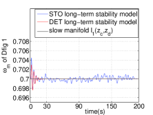
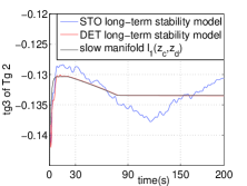
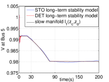
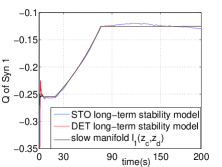
Figure 3: The trajectory comparisons of the stochastic long-term stability model and deterministic long-term stability model. Since all conditions of Theorem 2 are satisfied, the deterministic long-term stability model provides accurate approximations in terms of trajectories and stability assessment.

VI-B Numerical Example II

The second example is also a 14-bus system. There is one wind source and a corresponding DFIG at Bus 2. The Weibull distributed wind speed is characterized by parameters $k=1.51$, $\lambda=3.36$ and $\alpha=0.2575/3600$. In addition, there are four generators which are controlled by AVRs, TGs and OXLs. And there are three exponential recovery loads at Bus 9, Bus 10 and Bus 14 respectively. There are two continuous LTCs between Bus 4-9 and Bus 14-13, whose initial time delays are 30s. At 1s, there are three line losses between Bus 6-13, Bus 7-9 and Bus 6-11.

In this case, both the stochastic long-term stability model and the deterministic long-term stability model have voltage collapse, and the deterministic long-term stability model successfully captures the voltage instability. One of the sample paths of the stochastic model took 120.86s to simulate, while the deterministic model took 90.64s. The comparison between the trajectories of the stochastic long-term stability model and those of the deterministic long-term stability model as well as the slow manifold are shown in Fig. 4. Similarly, as all conditions of Theorem 2 are satisfied, the deterministic long-term stability model provides accurate approximations for the stochastic long-term stability model with correct stability assessment.

Physically speaking, as LTCs try to recover voltages at Bus 9 and Bus 13, OXLs at Generator 2 and Generator 4 are activated. LTCs require more power support from generators, however, OXLs protect generators from overheating, thus restrict power output. As the system can not meet the reactive power demand imposed by LTCs, voltages finally collapse.

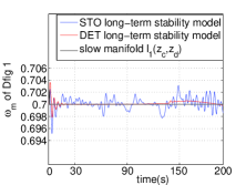
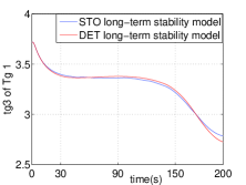
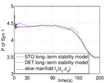
Figure 4: The trajectory comparisons of the stochastic long-term stability model and the deterministic long-term stability model. Since all conditions of Theorem 2 are satisfied, the deterministic long-term stability model provides accurate approximations in terms of trajectories and stability assessment that the system is long-term unstable.

VI-C Numerical Example III

The last example is a larger system which has 145 buses[33]. There are 6 DFIGs driven by different wind sources. Besides, there are 50 synchronous generators each of which is controlled by AVR, and Generator 10-Generator 20 are also controlled by TGs. There are OXLs at Generator 1-Generator 6 whose initial time delays are 50s. Additionally, there are 5 continuous LTCs between Bus 1-33, Bus 1-5, Bus 79-95, Bus 79-92, Bus 60-95 respectively. All LTCs have initial time delays of 50s. At 0.5s, there are three line losses including Bus 94-95, Bus 94-138 and Bus 95-138.

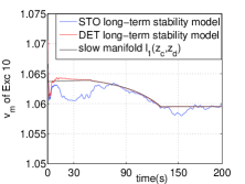
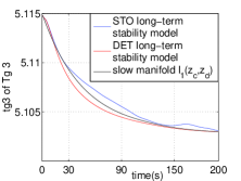
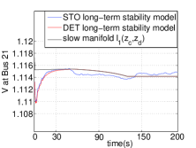
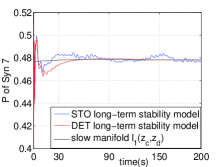
Figure 5: The trajectory comparisons of the stochastic long-term stability model and the deterministic long-term stability model. The deterministic long-term stability model provides accurate approximations for both trajectories and stability assessment.

The stochastic long-term stability model took 145.71s to simulate, while the deterministic long-term stability model took 91.18s. The comparison of the trajectories of the stochastic long-term stability model and those of the deterministic long-term stability model is shown in Fig. 5. Slow manifold of the deterministic model is also labelled. The simulation results show that the deterministic long-term stability model is able to provide accurate approximations for the stochastic long-term stability model with correct stability assessment, as all conditions of Theorem 2 are satisfied.

VII Conclusions and Perspectives

In this paper, we have incorporated the Weibull-distributed model of wind speed proposed in [21] into the power system dynamic model for long-term stability analysis. Under the SDE formulation, we have theoretically shown that the stochastic model can be approximated by a corresponding deterministic model for stability analysis under mild conditions. The proposed deterministic model takes much less time than the stochastic model, while is able to provide accurate stability assessments for the stochastic model.

This paper may represent the first attempt to apply the singular perturbation method for stochastic differential equations in power system stability research. The proposed methodology seems promising for stability analysis as the analytical results developed are not limited by the statistic properties of wind power, specific system models, penetration level and so forth. More particularly, the proposed method can accommodate wind speed models with different distributions like Rayleigh distribution, Lognormal distribution, Gamma distribution, etc. As a systematic method to model power systems as SDEs has been proposed in [22], we believe that the analytical results in this paper can be readily generalized, and thus provide a unified framework to conduct stability analysis for systems with uncertainties arising from load variations and other renewable energies.

As the integration of wind power continues to grow, the concerns about its stability impacts outstand. Practically speaking, power system operations on one hand concern about the variability of wind power, whereas on the other hand regard the wind power as constant in stability analysis to reduce the computational cost. The theory-based method proposed in the paper takes the statistic properties of wind power into account, and meanwhile does not increase the computational burden. Specifically, the computational cost for the proposed method is the same as the model using constant wind speed, which has been widely applied [9]-[15]; the proposed deterministic model can also be easily incorporated in any dynamic model originally used in the time domain simulation. In addition, the analytical results in the paper provide an answer to the question that when the variability of wind power needs to be considered in long-term stability study, and when it does not. Those results will give a practical guidance for power system stability assessments if efficient numerical schemes can be developed to check the sufficient conditions presented in Theorem 2. For other future works, an extension of the proposed method to the stochastic long-term stability model with discrete variables is expected. In addition, the proposed method can be further improved by applying the QSS model [2][3]. As such, the QSS model is able to incorporate wind generation into the formulation, and thus provides a more efficient computational tool to conduct long-term stability analysis for power grids with wind power. This extension of the QSS model may be a valuable advance in dynamic stability analysis, considering the wide industry applications of the QSS model and the continuous increasing of wind penetration. The analytical results proposed in this paper will be the foundation for those exciting subsequent works.

Appendix A singular perturbation theory for SDE

We consider the following stochastic system:

$$d{z} = f(z,x)dt+\bar{\sigma}Q(z,x)dW\qquad\quad z\in\mathbb{R}^{n_{z}}$$ (36)

$$d{x} = \frac{1}{\epsilon}g(z,x)dt+\frac{\sigma}{\sqrt{\epsilon}}G(z,x)dW\qquad x\in\mathbb{R}^{n_{x}}$$

where $W$ denotes a $k$-dimensional standard Wiener process, and $Q\in\mathbb{R}^{n_{z}\times k}$, $G\in\mathbb{R}^{n_{x}\times k}$ are matrix-valued functions. We are interested in the case that $\bar{\sigma}$ does not dominate $\sigma$, i.e., $\bar{\sigma}=\rho\sigma$ where $\rho$ is uniformly bounded above in $\epsilon$.

Assumption 2.

2.1 In some open connected set $D\subset\mathbb{R}^{n_{z}}\times\mathbb{R}^{n_{x}}$, $f\in C^{2}(D,\mathbb{R}^{n_{z}})$, $g\in C^{2}(D,\mathbb{R}^{n_{x}})$ and $Q\in C^{1}(D,\mathbb{R}^{n_{z}\times k})$, $G\in C^{1}(D,\mathbb{R}^{n_{x}\times k})$. $f$, $g$, $Q$, $G$ and all their partial derivatives up to order 2, respectively 1, are uniformly bounded in norm in $D$.

2.2 The slow manifold $x=j(z)$ where $z\in D_{0}\subset\mathbb{R}^{n_{z}}$ of deterministic system (14) is a stable component of constraint manifold $\Gamma$.

2.3 The diffusion matrix $G(z,j(z))G(z,j(z))^{T}$ is uniformly positive definite in $z\in D_{0}$.

Theorem 2.4 in [25] which is reviewed as Theorem 3 as below states that under Assumption 2, the sample path of system (36) are concentrated in an ellipsoidal layer surrounding the invariant manifold $j^{\star}(z,\epsilon)$ of system (14):

$$M(h)=\{(z,x):\langle(x-j^{\star}(z,\epsilon)),J^{\star}(z,\epsilon)^{-1}(x-j^{\star}(z,\epsilon))\rangle<h^{2}\}$$ (37)

up to time $t$, with a probability roughly like $1-(t^{2}/\epsilon)e^{-h^{2}/2\sigma^{2}}$. In particular, $J^{\star}(z,\epsilon)$ describing the cross section of the ellipsoid is well defined under Assumption 2. Refer to Section 2.3 of [25] or Chapter 5.1.1 of [24] for more details.

The following theorem shows that the sample paths of the stochastic system (36) are concentrated in a $\sigma$-neighborhood of invariant manifold $j^{\star}(z,\epsilon)$ of the deterministic system (14).

Theorem 3[25]: Under Assumption 2, for some fixed $\epsilon_{0}>0$, $h_{0}>0$, there exist $\delta_{0}>0$, a time $\tau_{1}$ of order $\epsilon|\mbox{log}h|$ such that whenever $\delta\leq\delta_{0}$, if an initial condition of stochastic system (36) $(z(0),{x}(0))$ where $z(0)\in D_{0}$ satisfies $(z(0),{x}(0))\in M(\delta)$, then for $\tau\geq\tau_{1}$, the following relation

$$\mathbb{P}\{\exists s\in[\tau_{1},\tau]:(z(\tau),{x}(\tau))\notin M(h)\}$$

$$\leq C_{n_{z},n_{x}}(\tau,\epsilon)e^{\frac{-h^{2}}{2\sigma^{2}}(1-O(h)-O(\epsilon))}$$ (38)

holds for all $\epsilon\leq\epsilon_{0}$, $h\leq h_{0}$, where coefficient $C_{n_{z},n_{x}}(\tau,\epsilon)=[C^{n_{z}}+h^{-n_{x}}](1+\frac{\tau}{\epsilon^{2}})$ is linear time-dependant.

A matching lower bound given in Theorem 2.4 of [25] shows that the above bound is sharp in the sense that it captures the correct behaviour of the probability.

Remark 1: It is shown in Theorem 5.1.17 in [24] (Remark 2.7 and Lemma 3.4 in [25]) that the stochastic singular perturbed system (36) can be approximated by the reduced deterministic system:

$$dz=f(z,j^{\star}(z,\epsilon))dt$$ (39)

and the deviation between the solution of (39) and that of (36) is of order $\sigma\sqrt{\epsilon}$ up to Lyapunov time of system (39). That means $z_{D}(t)$ provides $O(\sigma\sqrt{\epsilon})$ approximation for $z(t)$, i.e., $|z(t)-z_{D}(t)|=O(\sigma\sqrt{\epsilon})$.

Appendix B cross section of $N(h)$

Following the deduction of $J^{\star}(z,\epsilon)$ in Section 2.3 of [25] or Chapter 5.1.1 of [24], we can readily obtain the following results. The cross section $L_{1}^{\star}(z_{c},z_{d},\epsilon)$ of $N(h)$ is the solution of the following slow-fast system:

$${z_{c}}^{\prime} = H_{c}(z,l_{1}^{\star}(z_{c},z_{d},\epsilon))$$ (40)

$$\epsilon{L_{1}}^{\prime} = A(z_{c},z_{d},\epsilon)L_{1}^{\star}+L_{1}^{\star}A(z_{c},z_{d},\epsilon)^{T}+\left[\begin{array}[]{cc}\kappa I_{n_{{x}}}&0\\ 0&I_{n_{w}}\end{array}\right]$$ (43)

where

$$A(z_{c},z_{d},\epsilon) = \partial_{\bar{x}}F(z_{c},{l_{1}^{\star}}(z_{c},z_{d},\epsilon))$$

$$-\epsilon\partial_{z_{c}}{l_{1}^{\star}}(z_{c},z_{d},\epsilon)\partial_{\bar{x}}H_{c}(z_{c},l_{1}^{\star}(z_{c},z_{d},\epsilon))$$

and $\kappa>0$ is a sufficiently small positive parameter.

Note that the exact expression of $L_{1}^{\star}(z_{c},z_{d},\epsilon)$ is not of interest and thus does not need to be calculated, and we only need to know that $L_{1}^{\star}(z_{c},z_{d},\epsilon)$ is well defined in this formulation.

Appendix C proof of theorem 2

Proof: According to Theorem 2, if the conditions that $h\gg\sigma$ and (i)-(ii) in Theorem 2 are satisfied, then after a time of order $\epsilon|\mbox{log}h|$, sample paths of the stochastic long-term stability model (30) are concentrated in $N(\sigma)$ which is a $\sigma$-neighborhood of the invariant manifold $l_{1}^{\star}(z_{c},z_{d},\epsilon)$. Particularly, the slow dynamics of the stochastic long-term stability model (30) are in the $O(\sigma\sqrt{\epsilon})$ neighborhood of the invariant manifold $l_{1}^{\star}(z_{c},z_{d},\epsilon)$ as explained in Remark 1. Hence, Eqn (34) and Eqn (35) hold only if trajectory of the deterministic long-term stability model moves along the invariant manifold $l_{1}^{\star}(z_{c},z_{d},\epsilon)$. On the other hand, from singular perturbation theory, we have that if the slow manifold $\bar{x}=l_{1}(z_{c},z_{d})$ is a stable component of the constraint manifold, then the invariant manifold $l_{1}^{\star}(z_{c},z_{d},\epsilon)=l_{1}(z_{c},z_{d})+O(\epsilon)$ exists for sufficiently small $\epsilon$. Moreover, if one more condition that the initial point of the deterministic long-term stability model lies inside the stability region of the initial short-term stability model is also satisfied, then there exists $\epsilon_{0}$ such that trajectory of the deterministic long-term stability model (31) moves along the invariant manifold $l_{1}^{\star}(z_{c},z_{d},\epsilon)$ for all $\epsilon\in(0,\epsilon_{0})$, $\tau\in[\tau_{1},\tau_{2}]$[23][32]. Thus Eqn (34) and Eqn (35) hold for all $\epsilon\in(0,\epsilon_{0})$, $\tau\in[\tau_{1},\tau_{2}]$. This completes the proof.

References

- [1] H. D. Chiang, Direct Methods for Stability Analysis of Electric Power Systems-Theoretical Foundation, BCU Methodologies, and Applications. New Jersey: John Wiley & Sons, Inc, 2011.
- [2] T. V. Cutsem, Voltage Stability of Electric Power Systems. Boston/London/Dordrecht: Kluwer Academic Publishers, 1998.
- [3] T. V. Cutsem, Voltage instability: phenomena, countermeasures, and analysis methods. Proceedings of the IEEE, vol 88, no. 2 pp. 208-227, 2000.
- [4] P. Kundur, Power System Stability and Control. New York: McGraw-Hill, Inc. 1994.
- [5] P. Kundur, J. Paserba, V. Ajjarapu, Definition and classification of Power System Stability. IEEE Transactions on Power Systems, Vol. 19, No. 2, pp. 1387-1401, May 2004.
- [6] G. K. Morison, B. Gao, and P. Kundur, Voltage stability analysis using static and dynamic approaches. IEEE Transactions on Power Systems, vol. 8, no. 3, pp. 1159-1171, 1993.
- [7] P. A. LÖf, D. J. Hill, S. Arnborg, G. Andersson, On the analysis of long-term voltage stability. International Journal of Electrical Power & Energy Systems, vol. 15, no. 4, pp. 229-237, 1993.
- [8] J. G. Slootweg, H. Polinder, and W. L. Kling, Dynamic modelling of a wind turbine with doubly fed induction generator. IEEE Power Engineering Society Summer Meeting, vol. 1, pp. 644-649, 2001.
- [9] R. R. Londero, C. M. Affonso, and J. P. A. Vieira,Long-term voltage stability analysis of variable speed wind generators. IEEE Transactions on Power Systems, vol. 30, no. 1, pp. 439-447, Jan. 2015.
- [10] R. R. Londero, C. M. Affonso, J. P. A. Vieira, and U. H. Bezerra, Impact of different DFIG wind turbines control modes on long-term voltage stability. 2012 3rd IEEE PES Innovative Smart Grid Technologies Europe (ISGT Europe), Berlin.
- [11] P. Ledesma, J. Usaola, and J. L. Rodriguez, Transient stability of a fixed speed wind farm. Renewable energy, vol. 28, no. 9, pp. 1341-1355, 2003.
- [12] L. Meegahapola, D. Flynn, Impact on transient and frequency stability for a power system at very high wind penetration. IEEE Power and Energy Society General Meeting, 2010.
- [13] D. Gautam, V. Vittal, and T. Harbour, Impact of increased penetration of DFIG-based wind turbine generators on transient and small signal stability of power systems. IEEE Transactions on Power Systems, vol 24, no. 3, pp. 1426-1434, Aug 2009.
- [14] E. Vittal, M. O’Malley, and A. Keane, Rotor angle stability with high penetrations of wind generation. IEEE Transactions on Power Systems, vol. 27, no. 1, pp. 353-362, 2012.
- [15] A. Kanchanaharuthai, V. Chankong, and K. Loparo, Transient stability and voltage regulation in power systems with renewable distributed energy resources. IEEE Energytech, May 2011.
- [16] T. Odun-Ayo, M. L. Crow, Structure-preserved power system transient stability using stochastic energy functions. IEEE Transactions on Power Systems, vol. 27, no. 3, pp. 1450-1458.
- [17] B. Yuan, M. Zhou, G. Li, and X. P. Zhang, Stochastic small-signal stability of power systems with wind power generation. IEEE Transactions on Power Systems, doi: 10.1109/TPWRS.2014.2353014.
- [18] H. Mohammed, C. O. Nwankpa, Stochastic analysis and simulation of grid-connected wind energy conversion system. IEEE Transactions on Energy Conversion, vol. 15, no. 1, pp. 85-90, 2000.
- [19] Y. C. Chen, A. D. Domínguez-García, A method to study the effect of renewable resource variability on power system dynamics. IEEE Transactions on Power Systems, vol. 27, no. 4, pp. 1978-1989.
- [20] F. Milano, Power System Analysis Toolbox Documentation for PSAT version 2.1.5, November 1, 2009.
- [21] R.Zárate-Miñano, M. Anghel, and F. Milano, Continuous wind speed models based on stochastic differential equations. Applied Energy, vol. 104, pp. 42-49, Apr. 2013.
- [22] F. Milano, R. Zarate-Minano, A Systematic Method to Model Power Systems as Stochastic Differential Algebraic Equations. IEEE Transactions on Power Systems, vol. 28, no. 4, pp. 4537 - 4544, Nov 2013.
- [23] H. Khalil, Nonlinear System, 3rd ed, New York: Macmillan Publishing Company, 2002.
- [24] N. Berglund, B. Gentz, Noise-induced phenomena in slow-fast dynamical systems: a sample-paths approach. Springer, 2006.
- [25] N. Berglund, B. Gentz, Geometric singular perturbation theory for stochastic differential equations. Journal of differential equations, vol. 191, no. 1, pp. 1-54, 2003.
- [26] M. I. Freidlin, J. Szücs, A. D. Wentzell, Random Perturbations of Dynamical Systems. New York: 2nd Edition, Springer, 1998.
- [27] C. Kuehn, A mathematical framework for critical transitions: Bifurcations, fast–slow systems and stochastic dynamics. Physica D: Nonlinear Phenomena 240.12, pp. 1020-1035, 2011.
- [28] V. Veukatasubramanian, H. Schattler and J. Zaborszky, Dynamics of Large Constrained Nonlinear Systems—A Taxonomy Theory Proc. IEEE, Vol. 83, pp. 1530-1561, November. 1995.
- [29] Luis F. C. Alberto, H. D. Chiang, Theoretical Foundation of CUEP Method for Two-Time Scale Power System Models. Power and Energy Society General Meeting, 2009.
- [30] N. Fenichel, Geometric singular perturbation theory for ordinary differential equations. Journal of Differential Equations, vol. 31, no. 1, pp. 53-98.
- [31] C. Lobry, T. Sari, Singular perturbations in control theory. Nonlinear Control and Applications, Hermann : Travaux en Cours 64, 2005b, pp. 151-177.
- [32] X. Z. Wang, H. D. Chiang, Analytical Studies of Quasi Steady-State Model in Power System Long-term Stability Analysis. IEEE Transactions on Circuits and Systems I: Regular Papers, Vol. 61, No. 3, pp. 943 - 956, March 2014.
- [33] R. Christie, ”Power Systems Test Case Archive,” Electrical Engineering dept., University of Washington, Apr. 2000. [Online]. Available: http://www.ee.washington.edu/research/pstca.