Higgs boson coupling to a new strongly interacting sector

Abstract

In the framework of strongly interacting dynamics for electroweak symmetry breaking, heavy composite particles may arise and cause observable effects, as they should couple strongly to the resulting Higgs boson and affect the signals that appear at one loop level. Here we study this expected behavior, contrasting it with current experimental knowledge. We work in a simple and generic scenario where the lowest lying composite states are the Higgs scalar doublet and a massive vector triplet. We use an effective chiral Lagrangian to describe the theory below the compositeness scale $\Lambda$, assumed to be $4\pi v\simeq\leavevmode\nobreak\ 3$ TeV. The effective theory contains the Standard Model spectrum and the extra composites. We determine the constraints on this scenario imposed by our current knowledge of the $Zb\bar{b}$ vertex, the $T$ and $S$ oblique parameters, and the recently measured Higgs mass and its diphoton decay rate. We found that the $T$ and $S$ parameters as well as the Higgs diphoton decay do not provide important constraints on the model. In contrast, the constraints arising from the $Zb\bar{b}$ vertex and from the Higgs mass at $126$ GeV are fulfilled only if the heavy vector resonances do not couple strongly with quarks, and at the same time the Higgs boson has a moderate but not too strong coupling to the heavy composite resonances.

I Introduction.

The recent discovery of the Higgs boson at the LHC atlashiggs ; cmshiggs ; newtevatron ; CMS-PAS-HIG-12-020 provides the opportunity to directly explore the mechanism of Electroweak Symmetry breaking. While this remarkable achievement implies severe constrains on many proposed extensions of the Standard Model, an additional sector beyond our current knowledge is still needed in order to explain the dynamical origin of the electroweak scale and its stability pdg . A specific question in this context is whether this new sector is weakly or strongly interacting Contino:2009ez . In the latter case, the Higgs boson is viewed as a composite state which must be accompanied by a plethora of new heavy composite particles Grojean:2009fd ; Contino:2010rs ; Panico:2015jxa . In general, it is expected that the lightest states produced by the strong dynamics would correspond to spin-0 and spin-1 particles Grojean:2009fd ; Contino:2010rs ; Panico:2015jxa . In these models the lightness of the Higgs can be explained in two different ways. One way is to consider the Higgs boson as a pseudo-Goldstone boson that appears after the breakdown of a suitable global symmetry Contino:2010rs ; Panico:2015jxa ; Barbieri:2007 ; Csaki:2008zd ; Contino:2012 ; Pomarol:2012 ; Pappadopulo:2013vca ; Montull:2013mla . A second way is to consider the Higgs boson as the modulus of an effective SU(2) doublet, where its lightness is due to particularities of the dynamics of the underlying theory Bardeen:1989ds ; ggpr ; Zerwekh:2006 ; Zerwekh:2010 ; Carcamo:2010 ; Carcamo:ggtoVV ; Carcamo:2011 ; Burdman:2011 ; Carcamo:2012 ; Bellazini:2012 ; Contino:2013kra ; Diaz:2013tfa ; Castillo-Felisola:2013jua ; Hernandez:2013zho ; Carcamo-Hernandez:2013ypa ; Carcamo-Hernandez:2015xka ; Pappadopulo:2014qza ; Foadi:2007ue ; Ryttov:2008xe ; Sannino:2009za ; Belyaev:2013ida ; Hapola:2011sd ; Foadi:2012bb . For instance, there are evidences that quasi-conformal strong interacting theories such as Walking Technicolor may provide a light composite scalar Foadi:2007ue ; Ryttov:2008xe ; Sannino:2009za ; Belyaev:2013ida ; Hapola:2011sd ; Foadi:2012bb . It has also been shown that, in the effective low energy theory, the composite scalar may develop a potential that reproduces the standard Higgs sector Bardeen:1989ds . In this scheme, the Electroweak Symmetry breaking is effectively described by a non zero vacuum expectation value of the scalar arising from the potential, just as in the Standard Model. However, additional composite particles, like vector resonances, may also be expected to appear in the spectrum. In such a scenario, the vector sector can be extended by introducing a composite triplet of heavy vector resonances. This is the path we follow in this paper.

In general, a composite Higgs boson is theoretically attractive because the underlying strong dynamics provides a comprehensive and natural explanation for the origin of the Fermi scale Grojean:2009fd ; Contino:2010rs ; Panico:2015jxa . However, the presence of the already mentioned additional composite states may, in principle, produce phenomenological problems. For instance one could expect that, at one loop level, they may produce sensible corrections to observables involving the Higgs boson. Consequently, an interesting quantity which can eventually reveal the influence of additional states is $\Gamma(h\rightarrow\gamma\gamma)$. In a previous work one of us studied this decay channel in a simple model with vector resonances and found it is in general agreement with current experimental measurements in the limit where the Higgs boson is weakly coupled to the new resonances Castillo-Felisola:2013jua . In this work, we want to go further and use this channel to investigate if the experimental results still allow for a Higgs boson strongly coupled to the new $SU\left(2\right)_{L}$ triplet of heavy vectors resonances. In order to be concrete and predictive, we describe the new sector by means of an effective model with minimal particle content. We use an effective chiral Lagrangian to describe the theory below the cutoff scale, assumed to be $\Lambda=4\pi v\sim 3$ TeV, which contains the Standard Model spectrum and the extra composites.

The content of this paper goes as follows. In section II we introduce our effective Lagrangian that describes the spectrum of the theory. In section III we discuss the implications of the $Zb\bar{b}$ constraint in our model. In section IV, we determine the $T$ and $S$ oblique parameters in our model and discuss the implications of our model for electroweak precision tests. Section V deals with the constraints arising from the Higgs diphoton decay rate and the requirement of having a composite scalar mass of $126$ GeV. In section VI we describe the different decay channels of the heavy vector resonances. Finally in Section VII, we state our conclusions.

II Lagrangian for a Higgs doublet and heavy vector triplet.

To determine whether the current experimental data still allows for Higgs boson strongly coupled to a composite sector, we start by formulating our strongly coupled sector by means of an effective theory based on the gauge group $SU\left(2\right)_{L}\times U\left(1\right)_{Y}$ with a $SU\left(2\right)_{L}$ triplet of heavy vectors in addition to the SM fields. The gauge symmetry of the Standard Model is broken when the electrically neutral component of the scalar doublet $\Phi$ acquires a vacuum expectation value. The model Lagrangian can be written as:

$$\tciLaplace = -\frac{1}{2g^{2}}\left\langle W_{\mu\nu}W^{\mu\nu}\right\rangle-\frac{1}{2g^{\prime 2}}\left\langle B_{\mu\nu}B^{\mu\nu}\right\rangle-\frac{1}{2g_{\rho}^{2}}\left\langle\rho_{\mu\nu}\rho^{\mu\nu}\right\rangle$$ (1)

$$+f^{2}\left\langle\rho_{\mu}\rho^{\mu}\right\rangle+\left(D_{\mu}\Phi\right)^{{\dagger}}D^{\mu}\Phi-\frac{\lambda}{4}\left(\Phi^{{\dagger}}\Phi\right)^{2}+\mu^{2}\Phi^{{\dagger}}\Phi$$

$$+\alpha_{1}\mathop{\mathrm{R}e}\left(\Phi^{{\dagger}}\rho^{\mu}D_{\mu}\Phi\right)+\alpha_{2}\mathop{\mathrm{I}m}\left(\Phi^{{\dagger}}\rho^{\mu}D_{\mu}\Phi\right)$$

$$+\beta_{1}\left\langle\rho_{\mu}\rho^{\mu}\right\rangle\Phi^{{\dagger}}\Phi+\beta_{2}\Phi^{{\dagger}}\rho_{\mu}\rho^{\mu}\Phi$$

$$+i\kappa_{0}\left\langle W^{\mu\nu}\left[\rho_{\mu},\rho_{\nu}\right]\right\rangle$$

$$+i\kappa_{1}\left\langle\rho^{\mu\nu}\left[\rho_{\mu},\rho_{\nu}\right]\right\rangle+\kappa_{2}\left\langle\left[\rho^{\mu},\rho^{\nu}\right]\left[\rho_{\mu},\rho_{\nu}\right]\right\rangle$$

$$+\frac{ig_{\rho q\overline{q}}}{2}\left(\overline{q}_{iL}\gamma^{\mu}q_{iL}\rho_{\mu}^{3}+\sqrt{2}V_{ij}\overline{u}_{iL}\gamma^{\mu}d_{jL}\rho_{\mu}^{+}+h.c\right)+...,$$

where all parameters appearing in Eq. (1) are dimensionless with the exception of $f$ and $\mu$, which have mass dimension. Furthermore, the omitted terms ($...$) are the extra terms such as the couplings of the SM gauge bosons with SM fermions as well as the couplings of the heavy vectors with SM leptons. Here $\left\langle{}\right\rangle$ denotes the trace over the $2\times 2$ matrices and the scalar doublet $\Phi$ contains the SM Higgs boson and the SM would-be-Goldstone bosons. The SM Higgs doublet is given as usual by:

$$\Phi=\left(\begin{array}[]{c}G^{+}\\ \frac{1}{\sqrt{2}}\left(v+h+i\eta\right)\end{array}\right)=\left(\begin{array}[]{c}\frac{1}{\sqrt{2}}\left(\omega+i\xi\right)\\ \frac{1}{\sqrt{2}}\left(v+h+i\eta\right)\end{array}\right),$$ (2)

where the effective fields $h$, $\eta$, $\omega$ and $\xi$ have zero vacuum expectation values.

The covariant derivate acting on the scalar doublet $\Phi$ can be written as follows:

$$D_{\mu}\Phi=\partial_{\mu}\Phi-\frac{i}{2}gW_{\mu}^{a}\tau^{a}\Phi-\frac{i}{2}g^{\prime}B_{\mu}\Phi.$$ (3)

Furthermore, the tensor $\rho_{\mu\nu}=D_{\mu}\rho_{\nu}-D_{\nu}\rho_{\mu}$ is written in terms of a covariant derivative of the field $\rho_{\mu}$ as follows:

$$D_{\mu}\rho_{\nu}=\partial_{\mu}\rho_{\nu}-\frac{i}{2}\left[W_{\mu},\rho_{\nu}\right],$$ (4)

where $\rho_{\mu}=g_{\rho}\rho_{\mu}^{a}\frac{\tau^{a}}{2}$ is a $SU\left(2\right)_{L}$ triplet of composite vector resonances, neutral under hypercharge, formed due to the underlying strong dynamics.

In view of the large number of parameters of the model [c.f Eq. (1)] and in order to make definite predictions, we assume that the interactions of the heavy vectors $\rho_{\mu}$ with themselves as well as with the SM gauge bosons have the same Lorentz structure as the interactions among the SM gauge bosons. Consequently, the heavy vectors will correspond to the gauge vectors of a hidden local symmetry, and the aforementioned assumption leads to the following constraint:

$$\kappa_{1}=2\kappa_{0}=2\kappa_{2}=\frac{1}{g_{\rho}^{2}}.$$ (5)

When the Higgs boson acquires a vacuum expectation value $\left\langle\Phi\right\rangle=\frac{1}{\sqrt{2}}\left(0,v\right)^{T}$, from Eq. (1) it follows that the squared mass matrices for the neutral and charged gauge bosons are given by:

$$M_{N}^{2} = \left(\begin{array}[]{ccc}\frac{g^{\prime 2}}{4}&-\frac{gg^{\prime}}{4}&\alpha_{2}\frac{g^{\prime}g_{\rho}}{8}\\ -\frac{gg^{\prime}}{4}&\frac{g^{2}}{4}&-\alpha_{2}\frac{gg_{\rho}}{8}\\ \alpha_{2}\frac{g^{\prime}g_{\rho}}{8}&-\alpha_{2}\frac{gg_{\rho}}{8}&\left(\beta_{1}+\frac{\beta_{2}}{2}\right)\frac{g_{\rho}^{2}}{2}+g_{\rho}^{2}\frac{f^{2}}{v^{2}}\end{array}\right)v^{2},$$ (9)

$$M_{C}^{2} = \left(\begin{array}[]{cc}\frac{g^{2}}{4}&-\frac{gg_{\rho}}{8}\left(\alpha_{2}+i\alpha_{1}\right)\\ -\frac{gg_{\rho}}{8}\left(\alpha_{2}-i\alpha_{1}\right)&\left(\beta_{1}+\frac{\beta_{2}}{2}\right)\frac{g_{\rho}^{2}}{2}+g_{\rho}^{2}\frac{f^{2}}{v^{2}}\end{array}\right)v^{2}.$$ (12)

Assuming $g_{\rho}f\gg 100$ GeV and considering all dimensionless couplings here of the same order of magnitude, the following expressions for the gauge boson masses are obtained:

$$M_{A} = 0,\quad M_{Z}\simeq\frac{\sqrt{g^{2}+g^{\prime 2}}}{2}v,\quad M_{W}\simeq\frac{gv}{2},$$

$$M_{\rho^{0}} \simeq M_{\rho^{\pm}}\simeq\sqrt{\beta_{1}+\frac{\beta_{2}}{2}+\frac{2f^{2}}{v^{2}}}\frac{g_{\rho}v}{\sqrt{2}}.$$ (14)

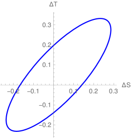
Figure 1: The interior of the ellipse in the $\Delta S-\Delta T$ plane is the experimentally allowed region at $95\%$CL from Ref. GFitter . The origin $\Delta S=\Delta T=0$ corresponds to the Standard Model value, with $m_{h}=126$ GeV and $m_{t}=176$ GeV.

III Constraints from the $Zb\bar{b}$ vertex

In this section we compute the one-loop correction to the $Zb\bar{b}$ vertex in our model, in order to set an upper bound on the direct coupling $g_{\rho q\overline{q}}$ of the heavy vectors with quarks. In the SM, the one-loop diagram containing the top quark induces a sizeable modification, $A_{bb}$, of the $Zb\bar{b}$ vertex from its tree level value:

$$\left(-\frac{1}{2}+\frac{\sin^{2}\theta_{W}}{3}+A_{bb}\right)\frac{g}{\cos\theta_{W}}Z_{\mu}\overline{b}_{L}\gamma^{\mu}b_{L},$$ (15)

where, in the large $m_{t}$ limit, the SM value for $A_{bb}$ is Barbieri:2007 :

$$A_{bb}^{\left(SM\right)}\simeq\frac{m_{t}^{2}}{16\pi^{2}v^{2}}.$$ (16)

In addition, the one-loop diagram containing a charged heavy vector resonance $\rho_{\mu}^{\pm}$, gives the following contribution to $A_{bb}$, up to corrections of order $\frac{m_{t}^{2}}{M_{\rho}^{2}}$:

$$\delta A_{bb}\simeq-\frac{41g_{\rho q\overline{q}}^{2}}{768\pi^{2}}.$$ (17)

Thus, the $A_{bb}$ parameter in our model is:

$$A_{bb}\simeq A_{bb}^{\left(SM\right)}\left(1-g_{\rho q\overline{q}}^{2}\frac{41}{48}\frac{v^{2}}{m_{t}^{2}}\right).$$ (18)

The experimental value of this quantity is $A_{bb}^{\left(\exp\right)}=0.923\pm 0.020$ whereas its SM value is $A_{bb}^{\left(SM\right)}=0.9347$ pdg . From these values we can extract bounds for $g_{\rho q\overline{q}}$, the direct coupling of the heavy vector resonances with quarks: the requirement of having $A_{bb}$ consistent up to $1\sigma$ with the experimental data yields the upper bound $g_{\rho q\overline{q}}\lesssim 0.14$, while a consistency within $3\sigma$ gives the looser bound $g_{\rho q\overline{q}}\lesssim\leavevmode\nobreak\ 0.21$.

IV Constraints from the T and S parameters

The inclusion of the extra composite particles also modifies the oblique corrections of the SM, the values of which have been extracted from high precision experiments. Consequently, the validity of our model depends on the condition that the extra particles do not contradict those experimental results. These oblique corrections are parametrized in terms of the two well known quantities $T$ and $S$. The $T$ parameter is defined as Peskin:1991sw ; Peskin:1991sw2 ; epsilon-approach ; epsilon-approach2 ; Barbieri:2004 ; Barbieri-book :

$$T=\frac{\Pi_{33}\left(0\right)-\Pi_{11}\left(0\right)}{M_{W}^{2}\alpha_{em}\left(m_{Z}\right)},$$ (19)

where $\Pi_{33}\left(0\right)$ and $\Pi_{11}\left(0\right)$ are the vacuum polarization amplitudes at $q^{2}=0$ for the propagators of the gauge bosons $\tilde{W}_{\mu}^{3}$ and $\tilde{W}_{\mu}^{1}$, respectively. Let us note, as stressed by Barbieri:2004 , that the gauge bosons $\tilde{W}_{\mu}^{a}$ ($a=1,2,3$) are linear combinations of the $W_{\mu}^{a}$ ($a=1,2,3$) SM gauge fields and the heavy vector resonances $\rho_{\mu}^{a}$ ($a=1,2,3$) since these fields have direct couplings with SM fermions. These linear combinations are defined in such a way that $\tilde{W}_{\mu}^{a}$ as well as $B^{0}$ are the only spin-1 fields (apart from the gluons) having gauge interactions with SM fermions. Consequently the fields $\tilde{W}_{\mu}^{a}$ ($a=1,2,3$) are defined as:

$$\tilde{W}_{\mu}^{a}=\frac{g}{\sqrt{g^{2}+g^{2}_{\rho q\overline{q}}}}W^{a}_{\mu}+\frac{g_{\rho q\overline{q}}}{\sqrt{g^{2}+g^{2}_{\rho q\overline{q}}}}\rho^{a}_{\mu},\hskip 28.45274pta=1,2,3.$$ (20)

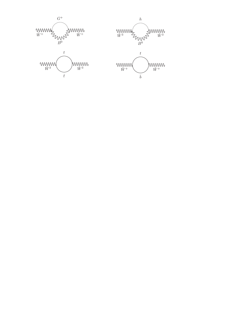
Figure 2: One loop Feynman diagrams contributing to the $T$ parameter.

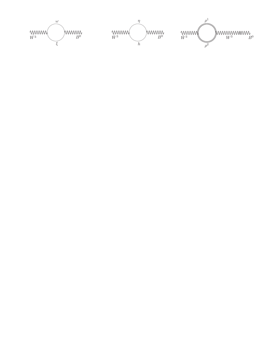
Figure 3: One loop Feynman diagrams contributing to the $S$ parameter. The first and second diagrams correspond to the SM contributions, whereas the third one is the contribution due to the heavy vector resonances.

In turn, the $S$ parameter is defined as Peskin:1991sw ; Peskin:1991sw2 ; epsilon-approach ; epsilon-approach2 ; Barbieri:2004 ; Barbieri-book :

$$S=\frac{4\sin^{2}\theta_{W}}{\alpha_{em}\left(m_{Z}\right)}\frac{g}{g^{\prime}}\frac{d}{dq^{2}}\Pi_{30}\left(q^{2}\right)\biggl{|}_{q^{2}=0},$$ (21)

where $\Pi_{30}\left(q^{2}\right)$ is the vacuum polarization amplitude for the propagator mixing of $\tilde{W}_{\mu}^{3}$ and $B_{\mu}$. The most important Feynman diagrams contributing to the $T$ and $S$ parameters are shown in Figures 2 and 3. We computed these oblique $T$ and $S$ parameters in the Landau gauge for the SM gauge bosons and would-be-Goldstone bosons, where the global $SU(2)_{L}\times U(1)_{Y}$ symmetry is preserved. We can separate the contributions to $T$ and $S$ from the SM and extra physics as $T=T_{SM}+\Delta T$ and $S=S_{SM}+\Delta S$, where

$$T_{SM} = -\frac{3}{16\pi\cos^{2}\theta_{W}}\ln\left(\frac{m_{h}^{2}}{m_{W}^{2}}\right)+\frac{3m_{t}^{2}}{32\pi^{2}\alpha_{em}\left(m_{Z}\right)v^{2}},\hskip 5.69046pt$$

$$S_{SM} = \frac{1}{12\pi}\ln\left(\frac{m_{h}^{2}}{m_{W}^{2}}\right)+\frac{1}{2\pi}\left[3-\frac{1}{3}\ln\left(\frac{m_{t}^{2}}{m_{b}^{2}}\right)\right],$$ (22)

while $\Delta T$ and $\Delta S$ contain all the contributions involving the extra particles.

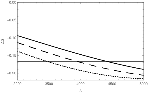
Figure 4: The $\Delta S$ parameter as a function of the cutoff $\Lambda$ for different values of the heavy vector masses $M_{\rho}$. Here we set $\alpha_{2}=g_{\rho}=1$ and $g_{\rho q\overline{q}}=0.14$. The curves from top to bottom correspond to $M_{\rho}=2.8$ TeV, $M_{\rho}=2.5$ TeV and $M_{\rho}=2.2$ TeV, respectively. The horizontal line corresponds to the minimum experimental value of the $\Delta S$ parameter at $95\%$CL for $\Delta T=0$.

The absence of quadratic divergences in the $T$ parameter requires that $\alpha_{1}=0$ in Eq. (1). In that case the dominant one-loop contribution to $\Delta T$ and $\Delta S$ in our model are:

$$\Delta T=\frac{3g_{\rho q\overline{q}}^{2}m_{t}^{2}}{32\pi^{2}\alpha_{em}\left(m_{Z}\right)\left(g^{2}+g_{\rho q\overline{q}}^{2}\right)v^{2}}+\frac{3}{16\pi\cos^{2}\theta_{W}}\left[\frac{\alpha_{2}g_{\rho}g_{\rho q\overline{q}}+g_{\rho q\overline{q}}^{2}}{g^{2}+g_{\rho q\overline{q}}^{2}}-\frac{\alpha_{2}^{2}g_{\rho}^{2}g_{\rho q\overline{q}}^{2}}{2g^{2}\left(g^{2}+g_{\rho q\overline{q}}^{2}\right)}\right]\ln\left(\frac{m_{h}^{2}}{m_{W}^{2}}\right),$$ (23)

$$\Delta S = \frac{1}{12\pi}\left(\frac{g-\sqrt{g^{2}+g_{\rho q\overline{q}}^{2}}}{\sqrt{g^{2}+g_{\rho q\overline{q}}^{2}}}-\frac{\alpha_{2}g_{\rho}g_{\rho q\overline{q}}}{2g\sqrt{g^{2}+g_{\rho q\overline{q}}^{2}}}\right)\ln\left(\frac{m_{h}^{2}}{m_{W}^{2}}\right)+\frac{1}{2\pi}\left[3-\frac{1}{3}\ln\left(\frac{m_{t}^{2}}{m_{b}^{2}}\right)\right]\left(\frac{g_{\rho q\overline{q}}^{2}}{g\sqrt{g^{2}+g_{\rho q\overline{q}}^{2}}}+\frac{g-\sqrt{g^{2}+g_{\rho q\overline{q}}^{2}}}{\sqrt{g^{2}+g_{\rho q\overline{q}}^{2}}}\right)$$ (24)

$$+\frac{\cos^{2}\theta_{W}\cos 2\theta_{W}}{3\pi}\left\{\frac{\Lambda^{2}}{M_{\rho}^{2}}-\frac{27}{8}-\frac{29}{4}\ln\left(\frac{\Lambda^{2}+M_{\rho}^{2}}{M_{\rho}^{2}}\right)+\frac{\left(34M_{\rho}^{2}\Lambda^{2}+27M_{\rho}^{4}\right)}{8\left(\Lambda^{2}+M_{\rho}^{2}\right)^{2}}+\frac{35\Lambda^{2}}{4\left(\Lambda^{2}+M_{\rho}^{2}\right)}\right\}$$

$$\times\left(\frac{g}{\sqrt{g^{2}+g_{\rho q\overline{q}}^{2}}}+\frac{g_{\rho}g_{\rho q\overline{q}}}{g\sqrt{g^{2}+g_{\rho q\overline{q}}^{2}}}\right).$$

Let us note that in our framework of strongly interacting effective theory, the $S$ parameter does not get tree level contributions because there are no kinetic mixing terms between the gauge fields and the heavy vectors. Here all couplings of the gauge fields with the heavy vectors are given by the mass terms. Using the expressions given above, it follows that for the benchmark point $\alpha_{2}=$ $g_{\rho}=1$ and $g_{\rho q\overline{q}}=0.14$ (so that the $Zb\bar{b}$ constraint is fullfilled), we get $\Delta T\simeq 4.24\times 10^{-2}$ and $-0.13\lesssim\Delta S\lesssim-0.08$ for heavy vector masses in the range $2.2$ TeV $\lesssim M_{\rho}\lesssim$ $3$ TeV. On the other hand, for the benchmark point $\alpha_{2}=$ $g_{\rho}=3.5\lesssim\sqrt{4\pi}$ and $g_{\rho q\overline{q}}=0.14$, we find $\Delta T\simeq-0.15$ and $-0.24\lesssim\Delta S\lesssim-0.15$, also for heavy vector masses in the range $2.2$ TeV $\lesssim M_{\rho}\lesssim$ $3$ TeV.

In Figs. 5.a and 5.b we show the allowed regions for the $\Delta T$ and $\Delta S$ parameters, for the two sets of values of $\alpha_{2}$, $g_{\rho}$ and $g_{\rho q\overline{q}}$ previously indicated. The ellipses denote the experimentally allowed region at 95% C.L., while the horizontal line shows the values of $\Delta T$ and $\Delta S$ in the model, as the mass of the heavy vectors $M_{\rho}$ is varied from $2.2$ TeV up to $3$ TeV. As shown, the $\Delta T$ and $\Delta S$ parameters in our model stay inside the ellipse in Fig. 1 for almost all the region of parameter space, and consequently the $T$ and $S$ constraints are easily fulfilled within our model, not imposing any restrictions on the model parameters other than the assumption that the heavy vector masses lie in the range $2.2$ TeV $\lesssim M_{\rho}\lesssim$ $3$ TeV. The lower bound comes from the ATLAS lower bound of $2.2$ TeV on direct searches for dijet resonances, while the upper bound is simply the assumed compositeness scale $\Lambda\sim 3$ TeV. Besides, the line in the figure is practically horizontal because the contribution of the heavy vectors to the $\Delta T$ parameter is very small. The natural smallness of the heavy vector contributions to the $\Delta T$ in our model is due to its form $\Delta T\sim v^{2}/M_{\rho}^{2}$, where the heavy vector masses $M_{\rho}$ are clearly much larger than the vacuum expectation value $v$.

Concerning $\Delta S$, even though its expression given in Eq. 24 exhibits a quadratic divergence with the cutoff, in the range of parameters of our model, the numerical values for $\Delta S$ are well within the experimentally allowed range. Indeed, Fig  4 shows the sensitivity of the $\Delta S$ parameter under variations of the cutoff $\Lambda$ for different values of the heavy vector masses $M_{\rho}$, namelly, $2.2$ TeV, $2.5$ TeV and $2.8$ TeV. Here we vary the cutoff $\Lambda$ from $3$ TeV to $5$ TeV. As can be seen from Fig  4, the $\Delta S$ parameter decreases when the cutoff is increased and from some values of the cutoff (depending on the heavy vector masses), it goes outside the allowed experimental limits but having the same order of magnitude. Consequently, one can say that the variation of the $\Delta S$ parameter with the cutoff is rather weak, thus making the $\Delta S$ parameter acquiring values of the same order of magnitude than the allowed experimental limits.

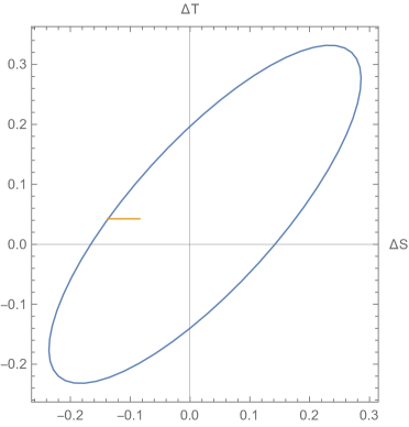
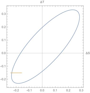
(7.a) $\alpha_{2}=$ $g_{\rho}=1$, $g_{\rho q\overline{q}}=0.14$                 (7.b) $\alpha_{2}=$ $g_{\rho}=3.5$, $g_{\rho q\overline{q}}=0.14$                                               

Figure 5: The $\Delta S-\Delta T$ plane in our model. The ellipses denote the experimentally allowed region at $95\%$CL taken from GFitter . The origin $\Delta S=\Delta T=0$ corresponds to the Standard Model value, with $m_{h}=126$ GeV and $m_{t}=176$ GeV. Figures a and b correspond to three different sets of values for the couplings $\alpha_{2}$, $g_{\rho}$, as indicated. The horizontal line shows the values of $\Delta S$ and $\Delta T$ in the model, as the mass of the heavy vectors $M_{\rho}$ varies over the range $2.2$ TeV $\leq M_{\rho}\leq$ $3$ TeV.

V Higgs diphoton rate and Higgs boson mass.

In the Standard Model, the $h\rightarrow\gamma\gamma$ decay mode is dominated by $W$ loop diagrams which can interfere destructively with the subdominant top quark loop. In our strongly coupled model, the $h\rightarrow\gamma\gamma$ decay receives additional contributions from loops with charged $\rho_{\mu}^{\pm}$, as shown in Fig. 6. The explicit form for the $h\rightarrow\gamma\gamma$ decay rate is:

$$\Gamma\left(h\rightarrow\gamma\gamma\right)=\frac{\alpha_{em}^{2}\,m_{h}^{3}}{256\pi^{3}v^{2}}\left|\sum_{f}N_{c}Q_{f}^{2}F_{1/2}\left(x_{f}\right)+F_{1}\left(x_{W}\right)+a_{h\rho^{+}\rho^{-}}F_{1}\left(x_{\rho}\right)\right|^{2},$$ (25)

where:

$$a_{h\rho^{+}\rho^{-}}\simeq\frac{g_{C}^{2}v^{2}}{M_{\rho^{\pm}}^{2}},\hskip 42.67912ptg_{C}^{2}=\left(\beta_{1}+\frac{\beta_{2}}{2}\right)\frac{g_{\rho}^{2}}{2}.$$ (26)

Here $x_{i}$ are the mass ratios $x_{i}=m_{h}^{2}/4M_{i}^{2}$, with $M_{i}=m_{f},M_{W}$ or $M_{\rho}$, respectively, $\alpha_{em}$ is the fine structure constant, $N_{C}$ is the color factor ($N_{C}=1$ for leptons, $N_{C}=3$ for quarks), and $Q_{f}$ is the electric charge of the fermion in the loop. From the fermion loop contributions we will keep only the dominant term, which is the one involving the top quark.

The dimensionless loop factors $F_{1/2}\left(x\right)$ and $F_{1}\left(x\right)$ (for particles of spin $1/2$ and 1 in the loop, respectively) are Ellis:1975ap ; HppBorn ; HppBorn0 ; HppAnnecy ; Gunion:1989we ; Spira:1997dg ; Djouadi2008 ; Marciano:2011gm :

$$F_{1/2}\left(x\right)=2\left[x+\left(x-1\right)f\left(x\right)\right]x^{-2},$$ (27)

$$F_{1}\left(x\right)=-\left[2x^{2}+3x+3\left(2x-1\right)f\left(x\right)\right]x^{-2},$$ (28)

with

$$f\left(x\right)=\begin{cases}\arcsin^{2}\sqrt{x},\hskip 14.22636pt\mathit{for}\hskip 5.69046ptx\leq 1\\ -\frac{1}{4}\left[\ln\left(\frac{1+\sqrt{1-x^{-1}}}{1-\sqrt{1-x^{-1}}}\right)-i\pi\right]^{2},\hskip 14.22636pt\mathit{for}\hskip 5.69046ptx>1.\end{cases}$$ (29)

In what follows, we want to determine the range of values for the mass $M_{\rho}$ of the heavy vector resonances, which is consistent with the Higgs diphoton signal strength measured by the ATLAS and CMS collaborations at the LHC. To this end, we introduce the ratio $R_{\gamma\gamma}$, which corresponds to the Higgs diphoton signal strength that normalises the $\gamma\gamma$ signal predicted by our model relative to that of the SM:

$$R_{\gamma\gamma} = \frac{\sigma\left(pp\rightarrow h\right)\Gamma\left(h\rightarrow\gamma\gamma\right)}{\sigma\left(pp\rightarrow h\right)_{SM}\Gamma\left(h\rightarrow\gamma\gamma\right)_{SM}}$$ (30)

$$\simeq \frac{\Gamma\left(h\rightarrow\gamma\gamma\right)}{\Gamma\left(h\rightarrow\gamma\gamma\right)_{SM}}.$$

This normalization for $h\rightarrow\gamma\gamma$ was also done in Refs. Wang ; Campos:2014zaa ; Hernandez:2015dga . Here we have used the fact that in our model, single Higgs production is also dominated by gluon fusion as in the Standard Model.

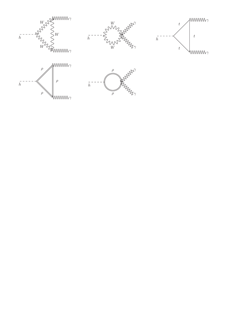
Figure 6: One loop Feynman diagrams in the Unitary Gauge contributing to the $h\rightarrow\gamma\gamma$ decay.

Fig. 7 shows the sensitivity of the ratio $R_{\gamma\gamma}$ under variations of the heavy vector masses $M_{\rho}$ for different values of the effective coupling $g_{C}$ (Figs. 7.a and 7.b correspond to $g_{C}=3.07$ and $g_{C}=1.26$, respectively). As previously mentioned, we only consider heavy vector masses above the ATLAS lower bound of $2.2$ TeV for dijet measurements, and up to the compositeness cutoff $\Lambda\sim 3$ TeV of our model. We see that an increase of the effective coupling $g_{C}$, which will correspond to a strong coupling of the heavy resonances with the Higgs boson, will give rise to an excess of events in the Higgs diphoton decay channel when compared with the SM expectation. In that case the Higgs diphoton signal strength will decrease from $1.27$ up to $1.14$ when the heavy vector masses are increased from $2.2$ TeV up to $3$ TeV, as indicated by Fig. 7.a. Requiring that the Higgs diphoton signal strength stays in the ballpark $0.9\lesssim R_{\gamma\gamma}\lesssim 1.44$ (the value obtained when we use the experimental errors of the recent CMS and ATLAS results, respectively), we find that heavy vector masses in the range $2.2$ TeV $\lesssim M_{\rho}\lesssim$ $3$ TeV are consistent with this requirement. On the other hand, as the effective coupling $g_{C}$ gets smaller, which implies that the coupling of the heavy resonances with the Higgs boson becomes weaker, the effect of these composite vector resonances in the Higgs diphoton decay rate turns out to be negligible, giving rise to a Higgs diphoton decay rate very close to that one predicted by the Standard Model, as indicated by Fig. 7.b.

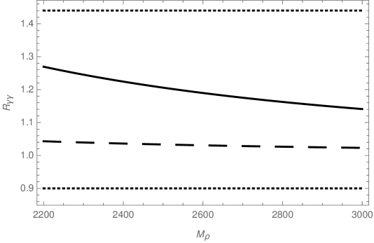
Figure 7: The Higgs diphoton signal strength $R_{\gamma\gamma}$ as a function of the mass $M_{\rho}$ of the heavy vectors for $g_{C}=3.07$ (solid curve) and $g_{C}=1.26$ (dashed curve). Here the values $g_{C}=3.07$ and $g_{C}=1.26$ correspond to the choices $\beta_{1}=\beta_{2}=1$, $g_{\rho}=\sqrt{4\pi}\simeq 3.5$ (maximum value allowed by perturbativity) and $\beta_{1}=\beta_{2}=1$, $g_{\rho}=1.45$, respectively (see Eq. 26 ). The horizontal lines are minimum and maximum values of the ratio $R_{\gamma\gamma}$ inside the 1$\sigma$ experimentally allowed range, determined by the experimental values and their uncertainties given by CMS and ATLAS, which are equal to $1.14^{+0.26}_{-0.23}$ and $1.17\pm 0.27$, respectively CMS2014 ; ATLAS2014 . Here we used the values given by ATLAS, which span a broader uncertainty range than CMS.

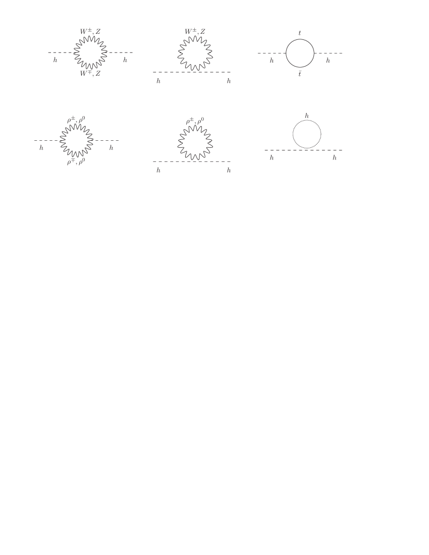
Figure 8: One loop Feynman diagrams in the Unitary Gauge contributing to the Higgs boson mass.

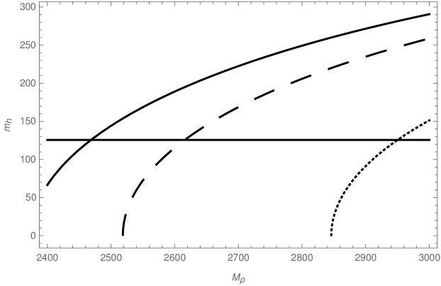
Figure 9: Higgs boson mass $m_{h}$ as function of the heavy vector mass $M_{\rho}$ for different values of the effective coupling $g_{C}$. The horizontal line corresponds to the value 126 GeV for the light Higgs boson mass. The solid, dashed and dotted curves correspond to the cases where $g_{C}$ is set to be equal to $1.20$, $1.26$ and $1.40$, respectively. The quartic Higgs coupling is taken to be equal to that of the Standard Model. Here we fix the tree level Higgs boson mass $\left(m_{h}\right)_{0}$ to be equal to $126$ GeV.

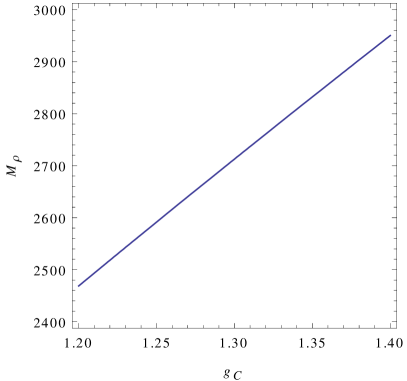
Figure 10: Correlation between the $g_{C}$ effective coupling and the heavy vector mass $M_{\rho}$ consistent with a Higgs boson mass of $126$ GeV. The quartic Higgs coupling is taken to be equal to that of the Standard Model.

Let us now determine the contraints on the effective coupling $g_{C}$ and the masses $M_{\rho}$ of the heavy vector resonances that can successfully accommodate a $126$ GeV Higgs boson mass. To this end, we proceed to compute the tree level and one loop level contributions to the Higgs boson mass $m_{h}$. The squared Higgs boson mass is given by:

$$m_{h}^{2}=\left(m_{h}^{2}\right)_{0}+\Sigma_{h},$$ (31)

where $\left(m_{h}^{2}\right)_{0}$ is the squared tree level Higgs boson mass and $\Sigma_{h}$ corresponds to the one loop level contribution, arising from Feynman diagrams containing spin-$0$, spin-$1/2$ and spin-$1$ particles in the internal lines of the loops. For the contribution from the fermion loops we will only keep the dominant term, which is the one involving the top quark. From the Feynman diagrams shown in Figure 8, it follows that the one loop level contribution to the squared Higgs boson mass is given by:

$$\Sigma_{h} \simeq 2F_{A}\left(M_{W}\right)+2F_{B}\left(M_{W}\right)+F_{A}\left(M_{Z}\right)+F_{B}\left(M_{Z}\right)$$ (32)

$$+2a_{h\rho^{+}\rho^{-}}^{2}F_{A}\left(M_{\rho}\right)+2a_{h\rho^{+}\rho^{-}}F_{B}\left(M_{\rho}\right)$$

$$+a_{h\rho^{0}\rho^{0}}^{2}F_{A}\left(M_{\rho}\right)+a_{h\rho^{0}\rho^{0}}F_{B}\left(M_{\rho}\right)$$

$$+F_{C}\left(m_{t}\right)+\frac{3}{4}\lambda F_{D}\left(m_{h}\right)$$

where $a_{h\rho^{0}\rho^{0}}\simeq a_{h\rho^{+}\rho^{-}}$ with the dimensionless parameter $a_{h\rho^{+}\rho^{-}}$ given by Eq. 26. In addition, the loop functions appearing in Eq. 32 are:

$$F_{A}\left(M\right) = \frac{M^{4}}{32\pi^{2}v^{2}}\left[\frac{\Lambda^{4}}{M^{4}}-\frac{6\Lambda^{2}}{M^{2}+\Lambda^{2}}+6\ln\left(\frac{\Lambda^{2}+M^{2}}{M^{2}}\right)\right],$$

$$F_{B}\left(M\right) = -\frac{M^{2}}{32\pi^{2}v^{2}}\left[\frac{\Lambda^{4}}{M^{2}}+6\Lambda^{2}-6M^{2}\ln\left(\frac{\Lambda^{2}+M^{2}}{M^{2}}\right)\right],$$

$$F_{C}\left(M\right) = \frac{3M^{2}}{4\pi^{2}v^{2}}\left[\allowbreak\Lambda^{2}-3M^{2}\ln\left(\frac{\Lambda^{2}+M^{2}}{M^{2}}\right)+\frac{3M^{2}\Lambda^{2}}{\Lambda^{2}+M^{2}}\right],$$

$$F_{D}\left(M\right) = -\frac{1}{16\pi^{2}}\left[\Lambda^{2}-M^{2}\ln\left(\frac{\Lambda^{2}+M^{2}}{M^{2}}\right)\right].$$ (33)

In Fig. 9 we show the sensitivity of the Higgs boson mass $m_{h}$ to variations in $M_{\rho}$ for $g_{C}=1.20$, $1.26$ and $1.40$ and the quartic Higgs coupling set to be equal to the Standard Model value. The Higgs boson mass $m_{h}$ is an increasing function of the heavy vector masses $M_{\rho}$. These Figures show that the heavy vector masses $M_{\rho}$ have an important effect of $m_{h}$. This is due to the fact that the one loop diagrams involving the heavy vector resonances and contributing to the Higgs boson mass are very sensitive to the cuttoff $\Lambda$, since they exhibit quartic and quadratic divergences that are not cancelled. Let us note that these heavy vector resonance one loop contributions to the Higgs boson mass involve trilinear and contact interactions, whose dominant terms are proportional to $\frac{g_{C}^{2}\Lambda^{4}}{M_{\rho}^{2}}$ and $\frac{g_{C}^{4}v^{2}\Lambda^{4}}{M_{\rho}^{4}}$, respectively, and consequently for larger vector masses, a stronger effective $g_{C}$ coupling is required to reproduce the $126$ GeV value for the Higgs boson mass, as shown in Fig. 10.

VI Decay channels of the heavy vectors

The current important period of LHC exploration of the Higgs properties and discovery of heavier particles may provide crucial steps to unravel the electroweak symmetry breaking mechanism. Consequently, we complement our work by studying the most relevant decay channels of the heavy vector resonances that could constitute direct signatures of our scenario at the LHC. To this end, we compute the two body decay widths of the heavy vectors. These widths, up to corrections of order $m_{h}^{2}/M_{\rho}^{2}$ and $M_{W}^{2}/M_{\rho}^{2}$ are:

$$\Gamma\left(\rho^{0}\rightarrow q\overline{q}\right) \simeq \frac{3g_{\rho q\overline{q}}^{2}}{96\pi}M_{\rho},$$

$$\Gamma\left(\rho^{+}\rightarrow u_{i}\overline{d}_{j}\right) = \Gamma\left(\rho^{-}\rightarrow\overline{u}_{i}d_{j}\right)\simeq\frac{3g_{\rho q\overline{q}}^{2}}{96\pi}\left|V_{ij}\right|^{2}M_{\rho},$$

$$\Gamma\left(\rho^{\pm}\rightarrow W^{\pm}h\right) = \Gamma\left(\rho^{0}\rightarrow Zh\right)\simeq\frac{\alpha_{2}^{2}g_{\rho}^{2}}{384\pi}M_{\rho},$$

$$\Gamma\left(\rho^{0}\rightarrow W^{+}W^{-}\right) = \Gamma\left(\rho^{\pm}\rightarrow W^{\pm}Z\right)\simeq\frac{\alpha_{2}^{2}g_{\rho}^{2}}{384\pi}M_{\rho}.$$ (34)

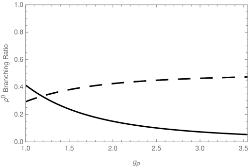
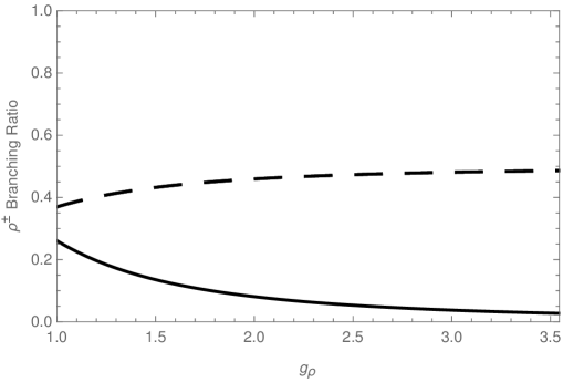
(11.a)

(11.b)

Figure 11: Branching ratios of the neutral (Fig. 11.a) and charged (Fig. 11.b) heavy vectors as functions of $g_{\rho}$ for $\alpha_{2}=1$ and $g_{\rho q\overline{q}}=0.14$. The solid curves correspond to the Branching ratios of the heavy vectors into quark pairs: a) $6Br\left(\rho^{0}\rightarrow q\overline{q}\right)$ and b) $3Br\left(\rho^{+}\rightarrow u\overline{d}\right)=3Br\left(\rho^{-}\rightarrow d\overline{u}\right)$, whereas the dashed curves correspond to the Branching ratios of the heavy vectors into a SM boson pair: a) $Br\left(\rho^{0}\rightarrow W^{+}W^{-}\right)=Br\left(\rho^{0}\rightarrow Zh\right)$ and b) $Br\left(\rho^{\pm}\rightarrow W^{\pm}Z\right)=Br\left(\rho^{\pm}\rightarrow W^{\pm}h\right)$.

Figure 11 displays the branching rations of the neutral (Fig. 11.a) and charged (Fig. 11.b) heavy vectors to quark-antiquark pairs and to a SM-like Higgs in association with a SM gauge boson, as a function of the composite vector resonance coupling $g_{\rho}$. This coupling is taken to range from $1$ to $3.5$ (value slightly lower than the maximum value $\sqrt{4\pi}$ allowed by perturbativity). Here we set $\alpha_{2}=1$ whereas the direct coupling of the heavy vector resonances with quarks $g_{\rho q\overline{q}}$ is set to be equal to $0.14$, the maximum value that keeps $A_{b\bar{b}}$ inside the $1\sigma$ experimentally allowed range, as described in Section III. One can notice that for low values of the $g_{\rho}$ coupling, the heavy vectors have a dominant decay mode into quark-antiquark pairs, comparable with the decay into a SM-like Higgs and SM gauge boson. On the other hand, when the value of the $g_{\rho}$ coupling is increased, the fermionic decay modes of the heavy vectors get suppressed, and the decay modes into a pair of SM Gauge bosons as well as into a SM-like Higgs and SM gauge boson become the dominant ones.

VII Conclusions.

We studied a framework of strongly interacting dynamics for electroweak symmetry breaking without fundamental scalars, by means of an effective theory based on the SM gauge group $SU\left(2\right)_{L}\times U\left(1\right)_{Y}$, with a $SU\left(2\right)_{L}$ triplet of heavy vectors. In this framework, it is assumed that the strong dynamics responsible for electroweak symmetry breaking gives rise to a composite triplet of heavy vectors and a composite scalar identified with the $126$ GeV Higgs boson, recently discovered at the LHC. It is assumed that the scalar and the heavy composite vectors are the only resonances that are lighter than the cufoff $\Lambda\simeq 4\pi v\sim 3$ TeV, so that the interactions among themselves and with the SM particles can be described by an effective chiral Lagrangian. The inclusion of the heavy vector resonances in the effective Lagrangian is done by considering them as gauge vectors of a hidden local symmetry. In this scenario, we determine the constraints arising from the $Zb\bar{b}$ vertex, from the $T$ and $S$ oblique parameters, and the constraints resulting from the measured Higgs diphoton decay rate and the Higgs mass of $126$ GeV. We found that the $Zb\bar{b}$ constraint at $1\sigma$ implies that the direct coupling of the heavy vector resonances with quarks should satisfy the upper bound $g_{\rho q\overline{q}}\lesssim 0.14$, which can be modified as $g_{\rho q\overline{q}}\lesssim 0.21$ by requiring that the $A_{bb}$ parameter that characterizes that constraint is inside the $3\sigma$ experimentally allowed range. Consequently the heavy vector resonances cannot strongly couple with quarks and therefore we found them to have a dominant decay mode into a SM-like Higgs and SM gauge boson in the region where the coupling $g_{\rho}$ of the strong sector is large. However, for low values of the $g_{\rho}$ coupling, these heavy vectors have a dominant decay mode into quark-antiquark pairs, comparable with the decays into a SM like Higgs and SM gauge boson as well as into a SM gauge bosons pair. Furthermore, we find that our model can easily accommodate the $T$ and $S$ oblique parameter constraints, as well as the Higgs diphoton decay rate constraints, in the whole relevant region $2.2$ TeV $\lesssim M_{\rho}\lesssim$ $3$ TeV for the heavy vector masses, for $g_{\rho}<\sqrt{4\pi}$ and $g_{\rho q\overline{q}}\lesssim 0.21$. We considered the heavy vector masses to be in the range $2.2$ TeV $\lesssim M_{\rho}\lesssim$ $3$ TeV, since our model is strongly interacting with a cutoff of $\Lambda\sim 3$ TeV, while consistency with the ATLAS dijet measurements yields the lower bound of $2.2$ TeV for the masses of the heavy vector resonances. In addition, we found that one loop effects are crucial to successfully reproduce the $126$ GeV Higgs boson mass. The requirement of having a $126$ GeV Higgs boson constrains the effective coupling $g_{C}$ and the mass $M_{\rho}$ of the heavy vectors to be in the ranges $1.2\lesssim g_{C}\lesssim$ $1.4$ and $2.47$ TeV $\lesssim M_{\rho}\lesssim$ $2.95$ TeV, respectively. In summary, an effective theory of strongly interacting dynamics for electroweak symmetry breaking, having in its particle spectrum the SM particles and a composite $SU\left(2\right)_{L+R}$ triplet of vector resonances, can successfully accommodate a light $126$ GeV Higgs boson, provided that the Higgs boson has a moderate but not too large coupling with heavy composite resonances. This framework is consistent with electroweak precision tests, Higgs diphoton decay rate constraints and the constraints arising from the $Zb\bar{b}$ vertex. We have shown that the current experimental data still allows for Higgs boson strongly coupled to a composite sector, assumed to include a composite $SU\left(2\right)_{L+R}$ triplet of vector resonances with a mass below the cutoff $\Lambda$. Finally, we should briefly comment that the tension between the effective $g_{C}$ coupling and the Higgs boson mass $m_{h}$ may be alleviated if the spectrum below the composite scale includes heavy fermions in addition to the vectors. Determining the effects of this enriched spectrum on the Higgs diphoton signal strength, the oblique $T$ and $S$ parameters, the $Zb\bar{b}$ vertex and the Higgs boson mass, requires an additional and careful analysis that we have left outside the scope of this work.

Acknowledgements

This work was supported in part by Conicyt (Chile) grant ACT-119 “Institute for advanced studies in Science and Technology”. C.D. also received support from Fondecyt (Chile) grant No. 1130617, and A.Z. from Fondecyt grant No. 1120346. A.E.C.H was partially supported by Fondecyt (Chile), Grant No. 11130115 and by DGIP internal Grant No. 111458.

References

- (1) G. Aad et al. [The ATLAS Collaboration], Phys. Lett. B716, 1 (2012) [arXiv:hep-ex/1207.7214].
- (2) S. Chatrchyan et al. [The CMS Collaboration], Phys. Lett. B716, 30 (2012) [arXiv:hep-ex/1207.7235].
- (3) T. Aaltonen et al. [CDF and D0 Collaborations], [arXiv:hep-ex/1207.6436].
- (4) The CMS Collaboration, CMS-PAS-HIG-12-020.
- (5) K. A. Olive et al. [Particle Data Group Collaboration], Chin. Phys. C 38, 090001 (2014).
- (6) R. Contino, Nuovo Cim. C 32N3-4, 11 (2009) [arXiv:0908.3578 [hep-ph]].
- (7) C. Grojean, PoS EPS -HEP2009, 008 (2009) [arXiv:0910.4976 [hep-ph]].
- (8) R. Contino, arXiv:hep-ph/1005.4269.
- (9) G. Panico and A. Wulzer, [arXiv:1506.01961 [hep-ph]].
- (10) R. Barbieri, B. Bellazini, V. S. Rychkov and A. Varagnolo, Phys. Rev. D 76 (2007) 115008 [arXiv:hep-ph/0706.0432].
- (11) C. Csaki, A. Falkowski and A. Weiler, JHEP 0809, 008 (2008) [arXiv:0804.1954 [hep-ph]].
- (12) R. Contino, D. Marzocca, D. Pappadopulo and R. Rattazzi, JHEP 1110 (2011) 081 [arXiv:1109.1570[hep-ph]].
- (13) A. Pomarol and F. Riva, JHEP 1208 (2012) 135 [arXiv:hep-ph/1205.6434].
- (14) D. Pappadopulo, A. Thamm and R. Torre, JHEP 1307, 058 (2013) [arXiv:1303.3062 [hep-ph]].
- (15) M. Montull, F. Riva, E. Salvioni and R. Torre, Phys. Rev. D 88, 095006 (2013) [arXiv:1308.0559 [hep-ph]].
- (16) W. A. Bardeen, C. T. Hill and M. Lindner, Phys. Rev. D 41, 1647 (1990).
- (17) G. F. Giudice, C. Grojean, A. Pomarol and R. Rattazzi, JHEP 0706 (2007) 045 [arXiv:hep-ph/0703164].
- (18) A. R. Zerwekh, Eur. Phys. J. C 46 (2006) 791 [arXiv:hep-ph/0512261].
- (19) A. R. Zerwekh, Mod. Phys. Lett. A A25 (2010), 423 [ arXiv:hep-ph/0907.4690].
- (20) A. E. Cárcamo Hernández and R. Torre [arXiv:1005.3809[hep-ph]], Nucl. Phys. B 841 (2010) 188.
- (21) A. E. Cárcamo Hernández, [arXiv:1008.1039[hep-ph]], Eur. Phys. J. C 72 (2012) 72:2154.
- (22) A. E. Cárcamo Hernández [arXiv:1108.0115[hep-ph]], PhD Thesis.
- (23) G. Burdman and C. E. F. Haluch, JHEP 1112 (2011) 038 [arXiv:1109.3914 [hep-ph]].
- (24) A. E. Cárcamo Hernández, C. O. Dib, N. Neill H and A. R. Zerwekh, JHEP 1202 (2012) 132 [ arXiv:hep-ph/1201.0878].
- (25) B. Bellazzini, C. Csaki, J. Hubisz, J. Serra and J. Terning, HEP 1211 (2012) 003 [arXiv:1205.4032[hep-ph]].
- (26) R. Contino, M. Ghezzi, C. Grojean, M. Muhlleitner and M. Spira, JHEP 1307 (2013) 035,arXiv:1303.3876 [hep-ph].
- (27) B. Diaz and A. R. Zerwekh, Int. J. Mod. Phys. A 28, 1350133 (2013) [arXiv:1308.0166 [hep-ph]].
- (28) O. Castillo-Felisola, C. Corral, M. González, G. Moreno, N. A. Neill, F. Rojas, J. Zamora and A. R. Zerwekh, Eur. Phys. J. C 73, 2669 (2013) [arXiv:1308.1825 [hep-ph]].
- (29) A. E. Cárcamo Hernández, C. O. Dib and A. R. Zerwekh, Nuovo Cim. C 036, no. 06, 177 (2013).
- (30) A. E. Cárcamo Hernández, C. O. Dib and A. R. Zerwekh, Eur. Phys. J. C 74, 2822 (2014) [arXiv:1304.0286 [hep-ph]].
- (31) A. E. Cárcamo Hernández, C. O. Dib and A. R. Zerwekh, arXiv:1503.08472 [hep-ph].
- (32) D. Pappadopulo, A. Thamm, R. Torre and A. Wulzer, arXiv:1402.4431 [hep-ph].
- (33) R. Foadi, M. T. Frandsen, T. A. Ryttov and F. Sannino, “Minimal Walking Technicolor: Set Up for Collider Physics,” Phys. Rev. D 76, 055005 (2007)
- (34) T. A. Ryttov and F. Sannino, “Ultra Minimal Technicolor and its Dark Matter TIMP,” Phys. Rev. D78, 115010 (2008)
- (35) For a recent review of modern DEWSB models see: F. Sannino, “Conformal Dynamics for TeV Physics and Cosmology,” Acta Phys. Polon. B40 (2009) 3533
- (36) A. Belyaev, M. S. Brown, R. Foadi and M. T. Frandsen, arXiv:1309.2097 [hep-ph].
- (37) T. Hapola and F. Sannino, Mod. Phys. Lett. A 26 (2011) 2313 [arXiv:1102.2920 [hep-ph]].
- (38) R. Foadi, M. T. Frandsen and F. Sannino, Phys. Rev. D 87 (2013) 095001 [arXiv:hep-ph/1211.1083
- (39) M. E. Peskin and T. Takeuchi, Phys. Rev. Lett. 65 (1990) 964;
- (40) M. E. Peskin and T. Takeuchi, Phys. Rev. D 46, 381 (1992).
- (41) G. Altarelli and R. Barbieri, Phys. Lett. B253 (1991) 161.
- (42) G. Altarelli, R. Barbieri and F. Caravaglios, Nucl. Phys. B405 (1993) 3.
- (43) R. Barbieri, A. Pomarol, R. Ratazzi and A. Strumia, Nucl. Phys. B 703 (2004) 127.
- (44) R. Barbieri, “Ten Lectures on Electroweak Interactions”, Scuola Normale Superiore, 2007, 81pp, [arXiv:0706.0684[hep-ph]]
- (45) J. R. Ellis, M. K. Gaillard and D. V. Nanopoulos, Nucl. Phys. B 106, 292 (1976).
- (46) A.I. Vaĭnshteĭn, M.B. Voloshin, V.I. Zakharov and M.A. Shifman, Sov. J. Nucl. Phys. 30 (1979) 711.
- (47) L. Okun, Leptons and Quarks, Ed. North Holland, Amsterdam, 1982.
- (48) M. Gavela, G. Girardi, C. Malleville and P. Sorba, Nucl. Phys. B193 (1981) 257.
- (49) J. F. Gunion, H. E. Haber, G. L. Kane and S. Dawson, “The Higgs Hunter’s Guide,” Front. Phys. 80, 1 (2000);
- (50) M. Spira, Fortsch. Phys. 46, 203 (1998);
- (51) A. Djouadi, Phys. Rept. 457, 1 (2008).
- (52) W. J. Marciano, C. Zhang and S. Willenbrock, Phys. Rev. D 85, 013002 (2012) [arXiv:1109.5304 [hep-ph]].
- (53) Lei. Wang and Xiao-Fang Han, Phys. Rev. D 86, 095007 (2012), [ arXiv:hep-ph/1206.1673].
- (54) M. D. Campos, A. E. Cárcamo Hernández, H. Pas and E. Schumacher, Phys. Rev. D 91, no. 11, 116011 (2015) [arXiv:1408.1652 [hep-ph]].
- (55) A. E. Cárcamo Hernández, I. d. M. Varzielas and E. Schumacher, arXiv:1509.02083 [hep-ph].
- (56) V. Khachatryan et al. [CMS Collaboration], Eur. Phys. J. C 74, no. 10, 3076 (2014) [arXiv:1407.0558 [hep-ex]].
- (57) G. Aad et al. [ATLAS Collaboration], Phys. Rev. D 90, no. 11, 112015 (2014) [arXiv:1408.7084 [hep-ex]].
- (58) M. Baak et al., “Updated Status of the Global Electroweak Fit and Constraints on New Physics,” Eur. Phys. J. C72 (2012) 2003, [arXiv:1107.0975[hep-ph]]