Study of underlying particle spectrum during huge X-ray flare of Mkn 421 in April 2013

Abstract

Context. In April 2013, the nearby (z=0.031) TeV blazar, Mkn 421, showed one of the largest flares in X-rays since the past decade.

Aims. To study all multiwavelength data available during MJD 56392 to 56403, with special emphasis on X-ray data, and understand the underlying particle energy distribution.

Methods. We study the correlations between the UV and gamma bands with the X-ray band using the z-transformed discrete correlation function. We model the underlying particle energy spectrum with a single population of electrons emitting synchrotron radiation, and do a statistical fitting of the simultaneous, time-resolved data from the Swift-XRT and the NuSTAR.

Results. There was rapid flux variability in the X-ray band, with a minimum doubling timescale of $1.69\pm 0.13$ hrs. There were no corresponding flares in UV and gamma bands. The variability in UV and gamma rays are relatively modest with $\sim 8\%$ and $\sim 16\%$ respectively, and no significant correlation was found with the X-ray light curve. The observed X-ray spectrum shows clear curvature which can be fit by a log parabolic spectral form. This is best explained to originate from a log parabolic electron spectrum. However, a broken power law or a power law with an exponentially falling electron distribution cannot be ruled out either. Moreover, the excellent broadband spectrum from $0.3-79$ keV allows us to make predictions of the UV flux. We find that this prediction is compatible with the observed flux during the low state in X-rays. However, during the X-ray flares, depending on the adopted model, the predicted flux is a factor of $2-50$ smaller than the observed one. This suggests that the X-ray flares are plausibly caused by a separate population which does not contribute significantly to the radiation at lower energies. Alternatively, the underlying particle spectrum can be much more complex than the ones explored in this work.

1 Introduction

According to the unification scheme of Active Galactic Nuclei (AGNs) by Urry & Padovani (1995), blazars are a subclass of AGNs with a relativistic jet aligned close to the line of sight. Blazars are further subdivided into BL Lacs and FSRQs where BL Lacs are characterized by the absence of (or very weak) emission lines. They show high optical polarization, intense and highly variable non-thermal radiation throughout the entire electromagnetic spectra in time scales extending from minutes to years, apparent super-luminal motion in radio maps, large Doppler factors and beaming effects. The broadband spectral energy distribution (SED) of blazars is characterized by two peaks, one in the IR - X-ray regime, and the second one in $\gamma$-ray regime. According to the location of the first peak, BL Lacs are further classified into Low energy peaked BL Lacs (LBLs) and High energy peaked BL Lacs (HBLs) (Padovani & Giommi, 1995). Both leptonic and hadronic models have been used to explain the broadband SED with varying degrees of success. The origin of the low energy component is well established to be caused by synchrotron emission from relativistic electrons gyrating in the magnetic field of the jet. However the physical mechanisms responsible for the high energy emission are still under debate. It can be produced either via inverse Compton (IC) scattering of low frequency photons by the same electrons responsible for the synchrotron emission (leptonic models), or via hadronic processes initiated by relativistic protons, neutral and charged pion decays or muon cascades (hadronic models). The seed photons for IC in leptonic models can be either the synchrotron photons itself (Synchrotron Self Compton, SSC) or from external sources such as the Broad Line Region (BLR), the accretion disc, the cosmic microwave background, etc (External Compton, EC). For a comprehensive review of these mechanisms, see Böttcher (2007).

Mkn 421 is the closest ($z=0.031$) and the most well studied TeV blazar. It was also the first detected extragalactic TeV source (Punch et al., 1992), and one of the brightest BL Lac objects seen in the UV and X-ray bands. It is a HBL, with the synchrotron spectrum peaking in the X-ray regime. Moreover, the X-ray emission is known to be highly correlated with the TeV emission (Błażejowski et al., 2005; K. Katarzynski et al., 2005; jie Qian et al., 1998), but like other HBLs, shows moderate correlation with the GeV emission (Li et al., 2013). It is highly variable and has been well studied during its flaring episodes by several authors (Aleksić et al., 2012; Shukla et al., 2012; Isobe et al., 2010; Krawczynski et al., 2001; Aleksić et al., 2010; Acciari et al., 2009; Ushio et al., 2009; Tramacere et al., 2009; Horan et al., 2009; Lichti et al., 2008; Fossati et al., 2008; Albert et al., 2007; Brinkmann et al., 2003). A detailed study of its quiescent state emission has been performed by Abdo et al. (2011) with the most well sampled SED till date.

During April 2013, Mkn 421 underwent one of the largest X-ray flares ever recorded in the past decade (Pian et al., 2014). The source was simultaneously observed by Swift and NuSTAR during this flaring episode, and we use these observations to study the spectral variations. To strengthen our study further, we supplement the X-ray information with other multiwavelength observations available.

The main focus of our work being the joint spectral fitting between the Nuclear Spectroscopic Telescope Array NuSTAR the Swift-XRT telescopes, and using this, we investigate the underlying particle energy spectrum. The high photon statistics during the flare, coupled with the excellent spectral response of Swift-XRT and NuSTAR gives us a rich X-ray spectrum from $0.3-79keV$ to explore. A study of the quiescent state of Mkn 421 using NuSTAR data was performed by Baloković et al. (2013). In Section 2 we describe the data reduction techniques from the various instruments. Section 3 lists the multiwavelength temporal results, while the X-ray spectral modelling is described in Section 4. We discuss the implications of the results in Section 5.

2 Multiwavelength Observations and Data Analysis

The huge X-ray flare of Mkn 421 during April 2013 ( 2013 April 10 to 21; MJD 56392$-$56403) is simultaneously observed by the NuSTAR and Swift X-ray and UV telescopes. The $\gamma$-ray behavior of this source during this flare was obtained by analyzing Fermi-LAT observations. In addition, we also include the X-ray observations by MAXI and optical observations by SPOL for the present study. The analysis procedures of these observations are described below.

2.1 Fermi-Large Area Telescope Observations

The Fermi-LAT data used in this work were collected covering the period of the X-ray outburst (MJD 56390$-$56403). The standard data analysis procedure as mentioned in the Fermi-LAT documentation was employed. Events belonging to the energy range 0.2$-$300 GeV and SOURCE class were used. To select good time intervals, a filter “DATA$\_$QUAL$>$0” && “LAT$\_$CONFIG==1” was chosen and only events with less than 105^∘ zenith angle were selected to avoid contamination from the Earth limb $\gamma$-rays. The galactic diffuse emission component gll_iem_v05_rev1.fits and an isotropic component iso_source_v05_rev1.txt were used as the background models. The unbinned likelihood method included in the pylikelihood library of Science Tools (v9r33p0) and the post-launch instrument response functions P7REP_SOURCE_V15 were used for the analysis. All the sources lying within 10^∘ region of interest (ROI) centered at the position of Mkn 421 and defined in the second Fermi-LAT catalog (Nolan et al., 2012), were included in the xml file. All the parameters except the scaling factor of the sources within the ROI are allowed to vary during the likelihood fitting. For sources between 10^∘ to 20^∘ from the centre, all parameters were kept frozen at the default values. The source was modelled by a power law as in the 2FGL catalog.

2.2 NuSTAR Observations

NuSTAR (Harrison et al., 2013) features the first focussing X-ray telescope to extend high sensitivity beyond 10 keV. There were 11 NuSTAR pointings between the aforementioned dates, the details of which are given in Table 1. The NuSTAR data were processed with the NuSTARDAS software package v.1.4.1 available within HEASOFT package (6.16). The latest CALDB (v.20140414) was used. After running nupipeline v.0.4.3 on each observation, nuproducts v.0.2.8 was used to obtain the lightcurves and spectra. Circular regions of 12 pixels centered on Mkn 421, and of 40 pixels centered at 165.96, 38.17 were used as source and background regions respectively. The spectra from the two detectors A and B were combined using addascaspec, and then grouped (using the tool grppha v.3.0.1) to ensure a minimum of 30 counts in each bin. To get strict simultaneity with Swift-XRT observations, observation id 60002023025 was broken into 4 parts 56393.15591890 to 56393.29538714, 56393.29538714 to 56393.91093765, 56393.91093765 to 56393.96788711 and 56393.96788711 to 56394.37822500 MJD.

2.3 Swift Observations

There were 15 Swift pointings between the aforementioned dates, the details of which are given in Table 2. Publicly available daily binned source counts were taken from the Swift-BAT webpage.

The XRT data (Burrows et al., 2005) were processed with the XRTDAS software package (v.3.0.0) available within HEASOFT package (6.16). Event files were cleaned and calibrated using standard procedures (xrtpipeline v.0.13.0), and xrtproducts v.0.4.2 was used to obtain the lightcurves and spectra. Standard grade selections of $0-12$ in the Windowed Timing (WT) mode are used. Circular regions of 20 pixels centered on Mkn 421 (at 166.113 and Dec 38.208) and of 40 pixels centered at 166.15, 38.17 were used as source and background regions respectively. For the observations affected by pileup (counts $>100c/s$) (Romano et al., 2006), an annular region of inner radius 2 pixels and outer 20 pixels was taken as the source region. The lightcurves were finally corrected for telescope vignetting and PSF losses with the tool xrtlccorr v.0.3.8. The spectra were grouped to ensure a minimum of 30 counts in each bin by using the tool grppha v.3.0.1.

Swift-UVOT (Roming et al., 2005) operated in imaging mode during this period, and for most of the observations, cycled through the UV filters UW1, UW2 and UM2. The tool uvotsource v.3.3 was used to extract the fluxes from each of the images using aperture photometry. The observed magnitudes were corrected for galactic extinction ($E_{B-V}=0.019$ mag) using the dust maps of Schlegel et al. (1998) and converted to flux units using the zero point magnitudes and conversion factors of Breeveld et al. (2011). The tool flx2xsp v.2.1 was used to convert the fluxes to pha files for use in XSPEC.

2.4 Other Multiwavelength data

Publicly available daily binned source counts were plotted for MAXI . As a part of the Fermi multiwavelength support program, the SPOL CCD Imaging/Spectropolarimeter at Steward Observatory at the University of Arizona (Smith et al., 2009) regularly observes Mkn 421. The publicly available optical V-band photometric and linear polarization data were downloaded from their website .

3 Multiwavelength Temporal Study

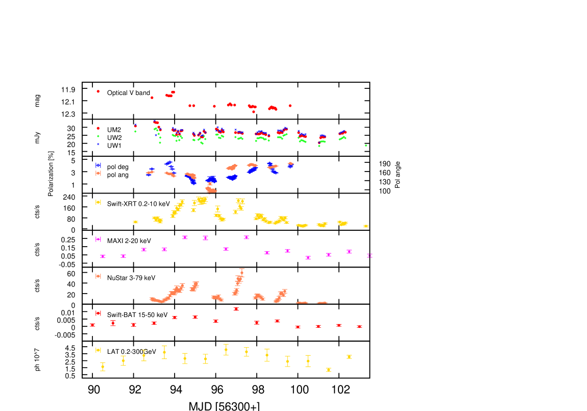
Figure 1: Multiwavelength lightcurve during MJD 56390 to 56403 showing : Panel 1: V band magnitude; Panel 2: UV flux in mJy; Panel 3: Degree and angle of optical polarization; Panel 4: Swift-XRT flux in counts/sec; Panel 5: MAXI flux in counts/sec; Panel 6: NuSTAR flux in counts/sec; Panel 7: Swift-BAT flux in counts/sec; Panel 8: Fermi-LAT flux in $ph/cm^{2}/sec$. One Swift-XRT (or NuSTAR) point is plotted for each snapshot.

The Multiwavelength lightcurve during the 10 days period, from optical to gamma ray energies, along with the optical polarization measurements, is plotted in Fig. 1. While there were two huge flares in X-rays (on MJD 56395 and 56397), where the flux went up by a factor of 10, the fluxes in the other bands were not very variable on the timescale of days. We compute the z-transformed discrete correlation using a freely available Fortran 90 code with the details of the method employed described in Alexander (1997). We find no lag between the soft ($0.3-10$ keV, Swift-XRT) and the hard X-ray ($3.0-79$ keV NuSTAR) bands. There is no correlation seen between the UV flux and the X-ray flux, ($zdcf_{max}=0.62\pm 2.3$, at a lag of $2.2$ days). Also, while the UV flux does not show correlation with the optical polarization ($zdcf_{max}=0.61\pm 1.1$, at a lag of $2.4$ days), the X-ray flux shows a tighter correlation ($zdcf_{max}=0.81\pm 0.6$, at a lag of $3.5$ days) with the latter. There was also a large change in the angle of polarization during the two X-ray flares.

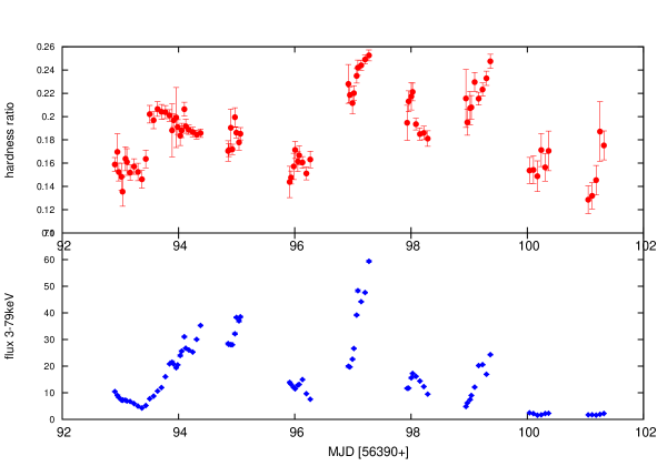
Figure 2: Plot of hardness ratio as observed by NuSTAR FPMA. The upper panel shows the hardness ratio, and the lower one, the flux(counts/sec). There is a trend of spectral hardening with flux.

The hardness ratios (computed here as the ratio between the 10 $-$ 79 keV count rate and the 3 $-$ 10 keV count rate (Tomsick et al., 2014)) are plotted in Fig. 2. A trend of spectral hardening with increasing flux (Spearman rank correlation, rs=$0.58$, $p=5.0\cdot 10^{-8}$), is observed and the same is often reported for this source (eg: Baloković et al., 2013; W. Brinkmann et al., 2001). Moreover, the correlation is much tighter during the rising part of the 2 flares (rs=$0.92$, $p=4.0\cdot 10^{-5}$). These interesting features advocate us to perform a more detailed spectral study, which we describe in Section 4.

The fractional variability amplitude parameter $F_{var}$ (Vaughan et al., 2003; Chitnis et al., 2009), computed on daily timescales, is used to quantify the multi-wavelength variability. It is calculated as

$$F_{var}=\sqrt{\frac{S^{2}-\sigma^{2}_{err}}{\bar{x}^{2}}}$$ (1)

where $\sigma^{2}_{err}$ is the mean square error, $\bar{x}$ the unweighted sample mean, and $S^{2}$ the sample variance. The error on $F_{var}$ is given as

$$\sigma_{F_{var}}=\sqrt{\left(\sqrt{\frac{1}{2N}}\cdot\frac{\sigma^{2}_{err}}{\bar{x}^{2}F_{var}}\right)^{2}+\left(\sqrt{\frac{\sigma^{2}_{err}}{N}}\cdot\frac{1}{\bar{x}}\right)^{2}}$$ (2)

Here, $N$ is the number of points.

The variability amplitude is the maximum for the X-ray bands ($F_{var}\sim 0.75\pm 0.10$), and significantly lower for the UV bands ($F_{var}\sim 0.08\pm 0.02$), suggesting that the emission may probably arise from different components in the two bands. The variability in the GeV range is also small ($F_{var}\sim 0.16\pm 0.07$). This goes against the general trend found in blazars that $F_{var}$ is the maximum for the $\gamma$-ray band and decreases with frequency (Zhang et al., 2005; Paliya et al., 2015).

We scan the Swift-XRT and the NuSTAR lightcurves for the shortest flux doubling timescale using the following equation (Foschini et al., 2011)

$$F(t)=F(t_{0}).2^{(t-t_{0})/\tau}$$ (3)

where $F(t)$ and $F(t_{0})$ are the fluxes at time $t$ and $t_{0}$ respectively, and $\tau$ is the characteristic doubling/halving time scale. The fastest observed variability in the NuSTAR band is $1.69\pm 0.08$ hours between MJD 97.06438 to 97.08573. This is comparable to the very fast variability observed in this source with the Beppo-SAX (Fossati et al., 2000a).

The above study is performed only for those periods where the flux difference is significant, at least at the $3\sigma$ level.

4 X-ray spectral analysis

The close simultaneity between Swift-XRT and NuSTAR observations allows us to do a joint spectral fitting using XSPEC package v.12.8.2. The time periods which have been fitted together are shown in Fig. 3. The bin widths are selected as one bin per Swift-XRT observation (except for Obs. id. 00035014062 and 00035014069, which last only for a few minutes) leading to 13 time bins which we denote as f1 - f13. The state f3 has no Swift-XRT data, whereas the state f13 has no NuSTAR data. Again in Table 3 we list the Swift-XRT and corresponding NuSTAR data which have been combined.

While fitting the broadband X-ray spectrum ($0.3-79$ keV), the XRT and the NuSTAR spectral parameters were tied to each other, except the relative normalization between the two instruments. To correct for the line of sight absorption of soft X-rays due to the interstellar gas, the neutral hydrogen column density was fixed at $N_{H}=1.92\times 10^{20}cm^{-2}$ (Kalberla et al., 2005).

4.1 Fitting the photon spectrum

It is known that the X-ray spectrum of Mkn 421 shows significant curvature (Fossati et al., 2000b; Massaro et al., 2004), and consistently we also noted that the data cannot be fitted satisfactorily by a simple power law. On the other hand, a power law with an exponential cutoff gives a much steeper curvature than observed, yielding to unacceptable fits. A sharp broken power law also gives large $\chi^{2}$ values in most cases, which suggests a smooth intrinsic curvature in the spectrum. So, following (Massaro et al., 2004; Tramacere et al., 2007) we fit the observed spectrum with a log parabola given by

$$dN/dE=K(E/E_{b})^{-\alpha_{s}-\beta_{s}log(E/E_{b,s})}$$ (4)

where $\alpha_{s}$ gives the spectral index at $E_{b,s}$. The point of maximum curvature, $E_{p,s}$ is given by

$$E_{p,s}=E_{b,s}10^{(2-\alpha_{s})/2\beta_{s}}$$ (5)

During fitting, $E_{b,s}$ is fixed at $1keV$. In Table 3, we give the resulting reduced $\chi^{2}$s for the case of the broken power-law and the log parabola models; while in Table 4, we give the fit parameters corresponding to the latter model.

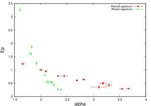
(a) $E_{p}$ vs $\alpha$

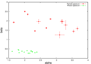
(b) $\beta$ vs $\alpha$

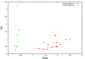
(c) $E_{p}$ vs $\beta$

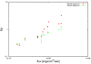
(d) $E_{p}$ vs flux

Figure 4: Cross plot of parameters for the logparabolic photon (green stars) and particle (red circles) spectrum respectively. The peak curvature $E_{p}$ clearly anti-correlates with $alpha$, and strongly correlates with the flux. However, there is no correlation between $E_{p}$ and the curvature parameter $\beta$, or between $\beta$ and $\alpha$.

Interestingly we noticed a strong anti-correlation between $\alpha_{s}$ and flux ($rs=-0.98$, $p<2.2\cdot 10^{-16}$), and a strong correlation between flux and $E_{p,s}$ ($rs=0.97$, $p<2.2\cdot 10^{-16}$) which implies that during flares, the spectral index at $1keV$ hardens and the peak of the spectrum shifts to higher energies. This behaviour of the source has often been reported (Massaro et al., 2004, 2008). In addition, we did not see any correlation between $\alpha_{s}$ and $\beta_{s}$ ($rs=-0.35$, $p=0.24$), which was seen by Massaro et al. (2004). We also noticed that there is no correlation observed between the curvature parameter $\beta$ and the peak of the curvature $E_{p}$ ($rs=0.63$, $p=0.02$). These cross plots are shown in Figure 4.

4.2 Emitting Particle Distribution

The excellent spectral resolution of NuSTAR gives us an unprecedented view of the high energy X-ray behavior beyond $20keV$. Coupled with Swift-XRT, we have, for the first time, an uninterrupted, well resolved spectrum from $0.3-79$ keV. This allows us to go beyond only fitting the photon spectrum with various spectral forms. Rather, in this work, we try to study the underlying particle distributions which give rise to the observed photon spectrum.

We consider the case where X-ray emission arise from a relativistic distribution of electrons emitting synchrotron radiation. The electrons are confined within a spherical zone of radius $R$ filled with a tangled magnetic field $B$. Due to relativistic motion of the jet, the radiation is boosted along our line of sight by a Doppler factor $\delta$. A good sampling of the entire SED from radio to $\gamma$-rays allows one to perform a reasonable estimation of these physical parameters (Tavecchio et al., 1998). For the case of synchrotron emission alone, $R$, $B$ and $\delta$ will only decide the spectral normalisation. On the other hand, the shape of the observed spectrum is determined by the corresponding form of the underlying particle spectrum. To obtain further insight into the emitting particle distribution, we developed synchrotron emission models with different particle distribution and incorporated them into XSPEC spectral fitting software. Particularly for this study, we consider the following particle distributions:

1. Simple power law (SPL): In this case, we assume the electron distribution to be a simple power law with a sharp high energy cutoff, given by

   $$N(\gamma)d\gamma=K\gamma^{-p}d\gamma,\mbox{\leavevmode\nobreak\ $\gamma<\gamma_{max}$\leavevmode\nobreak\ }\\$$ (6)

   Here $\gamma mc^{2}$ is the energy of the emitting electron, $p$ is the particle spectral index, $K$ is the normalization and $\gamma_{max}mc^{2}$ the cut-off energy. Among these parameters, $p$ and $\gamma_{max}$ are chosen as the free parameters.

2. Cutoff power law (CPL) : Here the underlying particle distribution is assumed to be a power law with index $p$ and an exponential cut-off above energy $\gamma_{m}mc^{2}$ given by

   $$N(\gamma)d\gamma=K\gamma^{-p}exp(\frac{\gamma}{\gamma_{m}})d\gamma\\$$ (7)

   For this distribution, $p$ and $\gamma_{m}$ are chosen as the free parameters.

3. Broken power law (BPL): The particle distribution in this case is described by a broken power law with indices $p_{1}$ and $p_{2}$ with a break at energy $\gamma_{b}$ given by

   $$N(\gamma)d\gamma=\left\{\begin{array}[]{ll}K\gamma^{-p_{1}}d\gamma,&\mbox{\leavevmode\nobreak\ $\gamma_{min}<\gamma<\gamma_{b}$\leavevmode\nobreak\ }\\ K\gamma^{(p_{2}-p_{1})}_{b}\gamma^{-p_{2}}d\gamma,&\mbox{\leavevmode\nobreak\ $\gamma_{b}<\gamma<\gamma_{max}$\leavevmode\nobreak\ }\end{array}\right.$$ (8)

   Here, $p_{1}$, $p_{2}$ and $\gamma_{b}$ are chosen as the free parameters.

4. Log parabola (LP): For this case, the particle distribution is chosen to be a log parabola, given by

   $$N(\gamma)d\gamma=K(\gamma/\gamma_{b})^{-\alpha_{p}-\beta_{p}log(\gamma/\gamma_{b})}d\gamma$$ (9)

   with $\alpha_{p}$ and $\beta_{p}$ chosen as the free parameters.

We fitted the observed combined X-ray spectrum from Swift-XRT and NuSTAR with the synchrotron emission due to these different particle distributions as given above. A poor fit statistic with large reduced $\chi^{2}$ is encountered for the case of SPL since it fails to reproduce the smooth curvature seen in almost all spectral states ($f1-f13$). For CPL, the statistics improved for many states (Table 3) with lowest reduced $\chi^{2}$ of 1.01 during state f3; whereas, the largest reduced $\chi^{2}$ is 1.41 for the state f6. The fit statistics improved considerably for many states for the case of BPL except for f6 and f8 corresponding to peak X-ray flare (Table 3). In Figure 5, we show the cross plot distribution of the power law indices, $p_{1}$ and $p_{2}$, of BPL model during different spectral states. The index $p_{1}$ is poorly constrained for the state f3 due to the absence of Swift-XRT observation during this period; whereas, for state f11 neither $p_{1}$ nor $p_{2}$ are well constrained due to the absence of NuSTAR observation. However, for most of the states, a strong correlation between $p_{1}$ and $p_{2}$ is observed ($rs=0.79$ and $p=0.0018$). Among all these particle distributions, the best statistics is obtained for the case of the LP model with the reduced $\chi^{2}$ decreased considerably during the flaring states, f5, f6 and f8 (Table 3). Further, the reduction of one free parameter in case of LP with respect to BPL enforces the latter to be the most preferred particle distribution. In Table 4, we give the best fit parameters for the case of the LP particle distribution. We see similar correlations as discussed in Section 4.1. In fact, there is a strong linear correlation ($p<1e-16$) between the corresponding parameters of the photon and the particle spectrum.

5 Discussions and Conclusions

In the present work, we performed a detailed study of the bright X-ray flare of Mkn 421 observed during April 2013 along with information available at other wavebands. We noticed the X-ray flare is not significantly correlated with the UV and, in addition, the variability amplitude of the former is considerably larger than the latter. This suggests that probably the X-ray and UV emission may belong to emission from different particle distributions.

A detailed spectral analysis of the X-ray observations over different time periods during the flare suggests the emission to arise due to synchrotron mechanism from log parabola particle distribution. Though this particle distribution can be statistically more appealing, a broken power law particle spectrum cannot be excluded. Further, we extended the best fit LP and BPL particle distributions to low energies and predicted the UV synchrotron flux. During low X-ray flux states, the predicted UV flux agrees reasonably well with the observed flux. However, at high X-ray flux states, the observed UV flux is significantly higher that the predicted one by a factor of $2-50$, with the larger deviations corresponding to the LP model. In addition, the variability of the predicted UV flux is much higher ($F_{var,pred}=1.10\pm 0.10$) than the one obtained from the observed UV flux. This study again questions the similar origin of X-ray and UV emission.

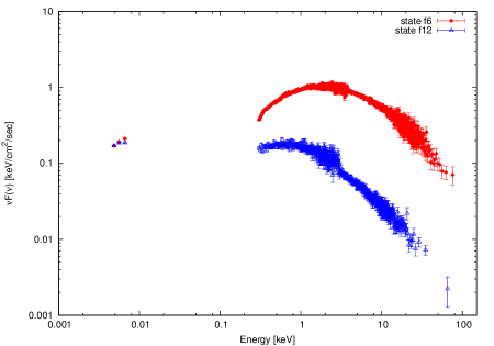
Figure 6: Observed X-ray and UV spectrum during two states. While the X-ray flux changes by more than a factor of 10, the UV flux remains constant.

A plausible interpretation of this inconsistency between X-ray and UV fluxes can be done by associating the UV emission from the putative accretion disk. However, such thermal emission from the disk was never a important contribution in the UV bands for Mkn 421 (Abdo et al., 2011), and the UV spectral detail is not sufficient enough to assert this interpretation (Figure 6). Alternatively, the underlying particle distribution can be more complex than the ones studied in this work. Nevertheless, such a particle distribution demands a concave spectrum which is not possible with our present understanding of particle acceleration (Sahayanathan, 2008). Hence, we attribute this unusual X-ray - UV behaviour of the source as a result of two population electron distribution. A similar conclusion was obtained by Aleksić et al. (2014) by studying a flare of the same source in March 2010. Such different electron distributions can be obtained if multiple emission regions are involved the emission process. If the flaring region is located at the recollimation zone of the jet, then a compact emission region can be achieved where the recollimation shock meets the jet axis (Tavecchio et al., 2011; Kushwaha et al., 2014). Alternatively, episodic particle acceleration suggested by Perlman et al. (2006) can be a reason for the second particle distribution. Perlman et al. (2005) have shown that this can also explain the relative less variability of the optical/UV bands as compared to the X-ray.

Pian et al. (2014) studied the same flare, starting from MJD 56397, with emphasis on INTEGRAL and Fermi-LAT data. They also found trends of spectral hardening with flux. However, unlike our results, the INTEGRAL spectral data could be well fit by a broken power law spectral form. They modelled the broadband SED with a simple one zone SSC model, and required large variations in the magnetic fields and Doppler factors to fit the SED of different states successfully. Also, our results do not match with that of Massaro et al. (2004) as we do not see any correlation between $\alpha_{s}$ and $\beta_{s}$. Thus, our results are inconsistent with statistical particle acceleration.

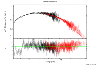
(a) cutoff power law, CPL

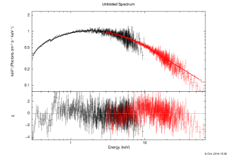
(b) broken power law, BPL

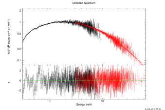
(c) log parabola, LP

Figure 7: Fitted spectrum and residuals for the three models for state f6. The differences start showing up above $50keV$

Our results indicate the potential of using broadband X-ray data to constrain the underlying particle spectrum and differentiate separate variable spectral components, especially if there are simultaneous data in other wavebands. Figure 7 shows the energy spectrum (in $\nu F_{\nu}$) and the residuals for the BPL, the CPL and the LP for the state f6. While the residuals show structure as a function of energy for energies $<0.7$keV, especially for the CPL and the BPL, the data and model agree within $10\%$ at these energies. Moreover, we also implemented a fit at energies $<0.7$keV and verified that our results do not change significantly. Thus, this effect is unlikely to be a serious source of error in this work. More importantly, there is a clear systematic deviation from the data for the BPL and the CPL at the higher energies, beyond $50keV$. The forthcoming satellite ASTROSAT (Singh et al., 2014), with its wide band X-ray coverage and simultaneous optical-UV measurement can be expected to make significant breakthroughs in this field.

Table 1: Details of Nustar pointings

obsid	start date and time	exposure (in sec)
60002023023	2013-04-10 20:53:07	118
60002023024	2013-04-10 21:26:07	5758
60002023025	2013-04-11 01:01:07	57509
60002023026	2013-04-12 20:11:07	441
60002023027	2013-04-12 20:36:07	7630
60002023029	2013-04-13 21:36:07	16510
60002023031	2013-04-14 21:41:07	15606
60002023033	2013-04-15 22:01:07	17278
60002023035	2013-04-16 22:21:07	20279
60002023037	2013-04-18 00:16:07	17795
60002023039	2013-04-19 00:31:07	15958

Table 2: Details of Swift pointings. The exposure times are rounded off to the nearest seconds

obsid	start date and time	xrt exposure	uvot exposure	bat exposure
00035014061	2013-04-10 02:04:58	1079	1066	1085
00080050016	2013-04-11 00:30:59	1118	1076	1128
00032792001	2013-04-11 03:41:30	3488	3468	3502
00080050017	2013-04-11 21:48:59	1449	1419	1453
00080050018	2013-04-12 00:33:59	8726	8635	8746
00080050019	2013-04-12 21:53:58	9546	9428	9572
00032792002	2013-04-14 00:38:59	6327	6253	6362
00035014063	2013-04-14 23:04:59	4942	4874	4965
00035014062	2013-04-15 23:07:59	534	522	540
00035014064	2013-04-16 00:43:59	10262	10108	10302
00035014065	2013-04-17 00:46:59	8842	8731	8857
00035014066	2013-04-18 00:49:59	6887	6798	6907
00035014067	2013-04-19 00:52:59	6132	6060	6152
00035014068	2013-04-20 00:55:59	5543	5482	4640
00035014069	2013-04-21 07:33:59	394	389	397

Table 3: Reduced $\chi^{2}$ values for the various time bins (f1 to f13), as marked in Figure 3, for the different models of the photon spectrum (broken power-law (bknpo) and log parabola (logpar)) and the particle spectrum (cutoff power law, broken power-law (bknpo) and logparabola) respectively. Observation ids of XRT and Nustar are also given.

State	Obs id		Photon spectrum		Particle spectrum
	XRT	Nustar	bknpo	logpar	CPL	BPL	LP
f1	00080050016	60002023024	1.27	1.02	1.07	1.06	1.03
f2	00032792001	60002023025 (a)	1.40	1.16	1.26	1.19	1.16
f3	-	60002023025 (b)	0.97	0.92	1.01	1.06	1.01
f4	00080050017	60002023025 (c)	1.22	1.04	1.08	1.07	1.05
f5	00080050018	60002023025 (d)	2.33	1.05	1.21	1.16	1.06
f6	00080050019	60002023027	2.93	1.08	1.41	1.39	1.09
f7	00032792002	60002023029	2.12	1.10	1.21	1.19	1.10
f8	00035014063	60002023031	2.45	1.14	1.20	1.31	1.13
f9	00035014064	60002023033	1.78	0.93	1.06	1.09	0.93
f10	00035014065	60002023035	1.75	1.10	1.09	1.10	1.10
f11	00035014066	60002023037	1.23	1.00	1.03	1.06	1.00
f12	00035014067	60002023039	1.14	1.01	1.08	1.02	1.01
f13	00035014068	-	1.07	1.07	1.04	1.07	0.92

Table 4: Best fit parameters of the log parabolic photon and particle spectrum respectively.

	Photon spectrum			Particle spectrum
state	$\alpha_{s}$	$\beta_{s}$	$E_{p,s}$	$\alpha_{p}$	$\beta_{p}$	$E_{p,p}$
f1	2.21 $\pm$ 0.02	0.39 $\pm$ 0.01	0.534 $\pm$ 0.027	$3.19\pm 0.06$	$1.96\pm 0.11$	$0.50\pm 0.04$
f2	2.21 $\pm$ 0.01	0.39 $\pm$ 0.01	0.543 $\pm$ 0.023	$3.18\pm 0.04$	$1.98\pm 0.09$	$0.50\pm 0.03$
f3	2.14 $\pm$ 0.05	0.27 $\pm$ 0.03	0.550 $\pm$ 0.074	$3.11\pm 0.14$	$1.25\pm 0.16$	$0.36\pm 0.06$
f4	1.92 $\pm$ 0.01	0.38 $\pm$ 0.02	1.254 $\pm$ 0.0630	$2.45\pm 0.06$	$1.97\pm 0.11$	$0.77\pm 0.06$
f5	1.82 $\pm$ 0.01	0.44 $\pm$ 0.01	1.585 $\pm$ 0.0229	$2.10\pm 0.02$	$2.35\pm 0.04$	$0.95\pm 0.03$
f6	1.80 $\pm$ 0.01	0.46 $\pm$ 0.01	1.634 $\pm$ 0.0205	$2.01\pm 0.02$	$2.50\pm 0.03$	$1.00\pm 0.02$
f7	2.08 $\pm$ 0.01	0.41 $\pm$ 0.01	0.805 $\pm$ 0.015	$2.82\pm 0.03$	$2.10\pm 0.04$	$0.64\pm 0.02$
f8	1.61 $\pm$ 0.01	0.37 $\pm$ 0.01	3.272 $\pm$ 0.0668	$1.66\pm 0.03$	$1.92\pm 0.04$	$1.23\pm 0.05$
f9	1.99 $\pm$ 0.01	0.33 $\pm$ 0.01	1.018 $\pm$ 0.0201	$2.69\pm 0.02$	$1.62\pm 0.03$	$0.61\pm 0.02$
f10	1.83 $\pm$ 0.01	0.30 $\pm$ 0.01	1.872 $\pm$ 0.039	$2.33\pm 0.02$	$1.46\pm 0.03$	$0.77\pm 0.02$
f11	2.33 $\pm$ 0.01	0.30 $\pm$ 0.01	0.280 $\pm$ 0.013	$3.55\pm 0.04$	$1.44\pm 0.07$	$0.29\pm 0.02$
f12	2.39 $\pm$ 0.01	0.33 $\pm$ 0.01	0.259 $\pm$ 0.012	$3.67\pm 0.04$	$1.59\pm 0.08$	$0.30\pm 0.02$
f13	2.25 $\pm$ 0.01	0.35 $\pm$ 0.03	0.445 $\pm$ 0.049	$3.30\pm 0.05$	$1.78\pm 0.23$	$0.43\pm 0.06$

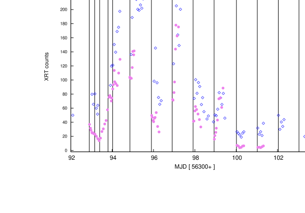
Figure 3: The 13 time bins for which spectra have been extracted.

Figure 5: Cross plot of the 2 indices of the broken power law particle spectrum. The green points are not from combined spectrum, but are NuSTAR only and Swift-XRT only (see text).