Landau levels and Shubnikov-de Haas oscillations in monolayer transition metal dichalcogenide semiconductors

Abstract

We study the Landau level spectrum using a multi-band $\mathbf{k}\cdot\mathbf{p}$ theory in monolayer transition metal dichalcogenide semiconductors. We find that in a wide magnetic field range the Landau levels can be characterized by a harmonic oscillator spectrum and a linear-in-magnetic field term which describes the valley degeneracy breaking. The effect of the non-parabolicity of the band-dispersion on the Landau level spectrum is also discussed. Motivated by recent magnetotransport experiments, we use the self-consistent Born approximation and the Kubo formalism to calculate the Shubnikov de-Haas oscillations of the longitudinal conductivity. We investigate how the doping level, the spin-splitting of the bands and the broken valley degeneracy of the Landau levels affect the magnetoconductance oscillations. We consider monolayer MoS₂ and WSe₂ as concrete examples and compare the results of numerical calculations and an analytical formula which is valid in the semiclassical regime. Finally, we briefly analyze the recent experimental results (Reference [18]) using the theoretical approach we have developed.

1 Introduction

Atomically thin transition metal dichalcogenides semiconductors (TMDCs) [1, 2, 3] are recognized as a material system which, due to its finite band gap, may have a complementary functionality to graphene, the best known member of the family of atomically thin materials. The experimental evidence that TMDCs become direct band gap materials in the monolayer limit [4] and that the valley degree of freedom [5] can be directly addressed by optical means [6, 7, 8, 9] have spurred a feverish research activity into the optical properties of these materials [10, 11, 12, 13]. Equally influential has proved to be the fabrication of transistors based on monolayer MoS₂ [14] which motivated a lot of subsequent research to understand the transport properties of these materials. Achieving good Ohmic contact to monolayer TMDCs is still challenging and this complicates the investigation of intrinsic properties through transport measurements. Nevertheless, significant progress has been made recently in reducing the contact resistance by e.g., using local gating techniques [15], phase engineering [16], making use of monolayer graphene as electrical contact [17, 18, 19], or selective etching procedure [20].

Our main interest here is to study magnetotransport properties of monolayer TMDCs. Unfortunately, the relatively strong disorder in monolayer TMDC samples have to-date hindered the observation of the quantum Hall effect. Nevertheless, the classical Hall conductance has been measured in a number of experiments [15, 18, 21, 22, 23] and was used to determine the charge density $n_{e}$ and to extract the Hall mobility $\mu_{H}$. In addition, three recent works have reported very promising progress in the efforts to uncover magnetic field induced quantum effects in monolayer TMDCs. Firstly, in Reference [24] the weak-localization effect was observed in monolayer MoS₂. Secondly, it was shown that in boron-nitride encapsulated mono- and few layer MoS₂ [18] and in few layer WSe₂ [20] it was possible to measure the Shubnikov-de Haas (SdH) oscillations of the longitudinal resistance. Both of these developments are very significant and can provide complementary informations: the weak localization corrections about the coherence length and spin relaxation processes [25, 26], whereas SdH oscillations about the cross-sectional area of the Fermi surface and the effective mass of the carriers.

Here we first briefly review the most important steps to calculate the LL spectrum in monolayer semiconductor TMDCs in perpendicular magnetic field using a multi-band $\mathbf{k}\cdot\mathbf{p}$ model[3]. We show that for magnetic fields of $B\lesssim 20\,$T a simple approximation can be applied to capture all the salient features of the LL spectrum. Motivated by recent experiments in MoS₂ [18] and WSe₂ [20], we use the LL spectrum and the self-consistent Born approximation (SCBA) to calculate the SdH oscillations of the longitudinal conductance $\sigma_{xx}$. We discuss how the intrinsic spin-orbit coupling and the valley degeneracy breaking (VDB) of the magnetic field affect the magnetoconductance oscillations. We also point out the different scenarios that can occur depending on the doping level.

2 Landau levels in monolayer TMDCs

Electronic states in the $K$ and $-K$ valleys are related by time reversal symmetry in monolayer TMDCs and hence in the presence of a magnetic field their degeneracy should be lifted. (Note that in the case of graphene the inversion symmetry, which is present there but not in monolayer TMDCs, ensures that in the non-interacting limit the LLs remain degenerate in the $K$ and $-K$ valleys.) Recently several works have calculated the Landau level (LL) spectrum of monolayer TMDCs using the tight-binding (TB) method [27, 28, 29] and found that the magnetic field can indeed lift the degeneracy of the LLs in different valleys. However, due to the relatively large number of atomic orbitals that is needed to capture the zero magnetic field band structure, for certain problems, such as the SdH oscillations of longitudinal conductance, the TB methodology does not offer a convenient starting point. On the other hand, a simplified two-band $\mathbf{k}\cdot\mathbf{p}$ model was used to predict unconventional quantum Hall effect [30] and to discuss valley polarization [31] and magneto-optical properties [32]. This model, however, did not capture the valley degeneracy breaking and was therefore in contradiction with the TB results and the considerations based on symmetry arguments.

We first show that the VDB in perpendicular magnetic field can be described by starting from a more general, seven-bands $\mathbf{k}\cdot\mathbf{p}$ model [3]. To this end we introduce an extended two-band continuum model which can be easily compared to previous works [30, 31, 32, 33]. We then show a relatively simple approximation for the LL energies which will prove to be useful for the calculation of the SdH oscillations in Section 3.

2.1 LLs from an extended two-band model

Our starting point to discuss the magnetic field effects in monolayer TMDCs is a seven-band $\mathbf{k}\cdot\mathbf{p}$ model (fourteen-band, if the spin degree is also taken into account), we refer the reader to Refs. [3] for details. In order to take into account the effects of a perpendicular magnetic field, one may use the Kohn-Luttinger prescription, i.e., we replace the wavenumbers $\mathbf{q}=(q_{x},q_{y})$ appearing in the seven-band model with operators: $\mathbf{q}\rightarrow\hat{\mathbf{q}}=\frac{1}{i}\boldsymbol{\nabla}+\frac{e}{\hbar}\mathbf{A}$, where $\mathbf{A}^{T}=(0,B_{z}x,0)$ is the vector potential in Landau gauge and $e>0$ is the magnitude of the electron charge. Note that due to this replacement $\hat{q}_{+}=\hat{q}_{x}+i\hat{q}_{y}$ and $\hat{q}_{-}=\hat{q}_{x}-i\hat{q}_{y}$ become non-commuting operators: $[\hat{q}_{-},\hat{q}_{+}]=\frac{2eB_{z}}{\hbar},$ where $|B_{z}|$ is the strength of the magnetic field and $[\dots]$ denotes the commutator. Working with a seven-band model is not very convenient and therefore one may want to obtain an effective model that involves fewer bands. This can be done using Löwdin-partitioning to project out those degrees of freedom from the seven-band Hamiltonian that are far from the Fermi energy. Since $\hat{q}_{+}$ and $\hat{q}_{-}$ are non-commuting operators, it is important to keep their order when one performs the Löwdin-partitioning. To illustrate this point we first consider a two-band model (four-band including spin) which involves the valence and the conduction bands (VB and CB). We will follow the notation used in Reference [3]. One finds that the low-energy effective Hamiltonian in a perpendicular magnetic field is given by

$$H_{\rm eff}^{\tau,s}=H_{0}+H_{\rm so}^{\tau,s}+H_{\mathbf{k}\cdot\mathbf{p}}^{\tau,s}$$ (1)

where $s=1$ ($s=-1$) denotes spin $\uparrow$ ($\downarrow$) and

$$H_{0}=\frac{\hbar^{2}}{2m_{e}}\frac{\hat{q}_{+}\hat{q}_{-}+\hat{q}_{-}\hat{q}_{+}}{2}+\frac{1}{2}g_{e}\mu_{B}B_{z}s_{z}$$ (2)

is the free electron term ($g_{e}\approx 2$ is the g-factor and $\mu_{B}$ is the Bohr magneton). Furthermore,

$$H_{\rm so}^{\tau,s}=\left(\begin{array}[]{cc}\tau\Delta_{\rm vb}s_{z}&0\\ 0&\tau\Delta_{\rm cb}s_{z}\end{array}\right)$$ (5)

describes the spin-orbit coupling in VB and CB ($s_{z}$ is a spin Pauli matrix) and $\tau=\pm 1$ for the $\pm K$ valleys. The $\mathbf{k}\cdot\mathbf{p}$ Hamiltonian $H_{\mathbf{k}\cdot\mathbf{p}}^{\tau,s}$ reads

$$H_{\mathbf{k}\cdot\mathbf{p}}^{\tau,s}=H_{\rm D}^{\tau,s}+H_{\rm as}^{\tau,s}+H_{3w}^{\tau,s}+H_{\rm cub}^{\tau,s},$$ (6)

where

$$H^{\tau,s}_{D}=\left(\begin{array}[]{cc}\varepsilon_{\rm vb}&\tau\,\gamma_{\tau,s}\hat{q}_{-}^{\tau}\\ \tau\,\gamma_{\tau,s}^{*}\hat{q}_{+}^{\tau}&\varepsilon_{\rm cb}\end{array}\right),$$ (7c)

$$H^{\tau,s}_{\rm as}=\left(\begin{array}[]{cc}\alpha_{\tau,s}\hat{q}_{+}^{\tau}\hat{q}_{-}^{\tau}&0\\ 0&\beta_{\tau,s}\hat{q}_{-}^{\tau}\hat{q}_{+}^{\tau}\end{array}\right),$$ (7f)

$$H^{\tau,s}_{3w}=\left(\begin{array}[]{cc}0&\kappa_{\tau,s}(\hat{q}_{+}^{\tau})^{2}\\ \kappa_{\tau,s}^{*}(\hat{q}_{-}^{\tau})^{2}&0\end{array}\right),$$ (7i)

$$H^{\tau,s}_{cub,1}=-\frac{\tau}{2}\left(\begin{array}[]{cc}0&\eta_{\tau,s}^{(1)}\hat{q}_{+}^{\tau}\hat{q}_{-}^{\tau}\hat{q}_{-}^{\tau}+\eta_{\tau,s}^{(2)}\hat{q}_{-}^{\tau}\hat{q}_{-}^{\tau}\hat{q}_{+}^{\tau}\\ (\eta_{\tau,s}^{(1)})^{*}\hat{q}_{+}^{\tau}\hat{q}_{+}^{\tau}\hat{q}_{-}^{\tau}+(\eta_{\tau,s}^{(2)})^{*}\hat{q}_{-}^{\tau}\hat{q}_{+}^{\tau}\hat{q}_{+}^{\tau}&0\end{array}\right).$$ (7l)

Here the operator $\hat{q}_{\pm}^{\tau}$ is defined as $\hat{q}_{\pm}^{\tau}=\hat{q}_{x}\pm i\tau\hat{q}_{y}$. The material specific properties are encoded in the parameters ${\varepsilon}_{\rm vb}$, ${\varepsilon}_{\rm cb}$ (band-edge energies in the absence of SOC), $\gamma_{\tau,s}$ (coupling between the VB and the CB) and $\alpha_{\tau,s}$, $\beta_{\tau,s}$, $\kappa_{\tau,s}$, $\eta_{\tau,s}^{(1)}$, $\eta_{\tau,s}^{(2)}$, which describe the effects of virtual transitions between the VB (CB) and the other bands in the seven-band model. In general, the off-diagonal material parameters $\gamma_{s,\tau}$, $\kappa_{s,\tau}$ and $\eta_{s,\tau}^{(1)}$, $\eta_{s,\tau}^{(2)}$ are complex numbers such that for the $-K$ valley ($\tau=-1$) they are the complex conjugates of the $K$ valley case ($\tau=1$). In the absence of a magnetic field, the material parameters appearing in Eqs. (7c) - (7l) can be obtained by, e.g., fitting the eigenvalues of $H_{\rm eff}^{\tau,s}$ to the band structure obtained from density functional theory (DFT) calculations. We refer to Reference [3] for the details of this fitting procedure and for tables containing the extracted parameters for monolayer semiconductor TMDCs. Here we only mention that such a fitting procedure yields real numbers which depend on the spin index $s$ but do not depend explicitly on the valley index $\tau$. (The parameters $\eta_{\tau,s}^{(1)}$ and $\eta_{\tau,s}^{(2)}$ cannot be obtained separately from fitting the DFT band structure, only their sum, $\eta_{\tau,s}$ can be extracted. Fortunately, as we will see below, the effect of $H^{\tau,s}_{cub,1}$ is very small in the magnetic field range we are primarily interested in. )

We note that a $\mathbf{k}\cdot\mathbf{p}$ model, similar to ours, was recently used in References [29, 33] to calculate the LL spectrum. There are two differences between our $\mathbf{k}\cdot\mathbf{p}$ Hamiltonian Eqs. (6) and the model in References [29, 33]. The first one is that higher order terms that would correspond to our $H^{\tau,s}_{3w}$ and $H^{\tau,s}_{cub,1}$ were not considered in References [29, 33]. We keep these terms in order to see more clearly the magnetic field range where the approximation discussed in Section 2.2 is valid. The second difference can be found in our $H^{\tau,s}_{\rm as}$ (7f) and the corresponding Hamiltonian used in [29, 33]. This difference can be traced back to the way the magnetic field is taken into account in the effective models that are obtained from multi-band Hamiltonians. In References [29, 33] first an effective zero field two-band model was derived and then in a second step the Luttinger-prescription was performed in this effective model. Therefore the terms which are $\sim q^{2}$ in the zero field case become $\sim\hat{q}_{+}\hat{q}_{-}+\hat{q}_{-}\hat{q}_{+}$ after the Luttinger-prescription. In contrast, as mentioned above, we perform the Luttinger prescription in the multi-band Hamiltonian and obtain the effective two-band model $H_{\rm eff}^{\tau,s}$ (1) in the second step. The two approaches may lead to different results because the operators $\hat{q}_{+}$, $\hat{q}_{-}$ do not commute and this should be taken into account in the Löwdin-partitioning which yields the effective two-band model.

The spectrum of $H_{\rm eff}^{\tau,s}$ can be calculated numerically using harmonic oscillator eigenfunctions as basis states. Taking $B_{z}>0$ for concreteness, one can see that the operators $a$ and $a^{\dagger}$ defined as $\hat{q}_{-}=\frac{\sqrt{2}}{l_{b}}a$, $\hat{q}_{+}=\frac{\sqrt{2}}{l_{b}}a^{\dagger}$, where $l_{B}=\sqrt{\hbar/(e|B_{z}|)}$, satisfy the bosonic commutation relation $[a,a^{\dagger}]=1$. (For $B_{z}<0$ one has to define $\hat{q}_{+}=\frac{\sqrt{2}}{l_{b}}a$, $\hat{q}_{-}=\frac{\sqrt{2}}{l_{b}}a^{\dagger}$). Therefore one can calculate the matrix elements of $H_{\rm eff}^{\tau,s}$ in a large, but finite harmonic oscillator basis and diagonalize the resulting matrix. For a large enough number of basis states the lowest eigenvalues of $H_{\rm eff}^{\tau,s}$ will not depend on the exact number of the basis states. Such a LL calculation is shown in Figure 1 for MoS₂ and in Figure 2 for WSe₂ (we have used the material parameters given in Reference [3]). One can see that the LLs in different valleys are not degenerate and that the magnitude of the valley degeneracy breaking is different in the VB and CB and for the lower and higher-in-energy spin-split bands. While the results in the VB are qualitatively similar for MoS₂ and WSe₂, considering the CB, for MoS₂ the valley splitting of the LLs is smaller in the higher spin-split band, whereas the opposite is true for WSe₂. This is a consequence of the interplay of the Zeeman term in Eq. (2) and other, band-structure related terms which lead to VDB. (For MoS₂ the valley splitting in the higher spin-split CB (purple and cyan lines) is very small for the material parameter set used in these calculations and can only be noticed for large magnetic fields.) One can also observe that in the CB the lowest LL is in valley $K$, whereas in the VB it is in valley $-K$.

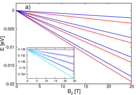
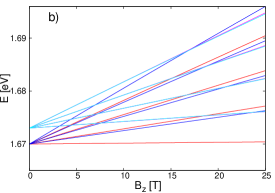
Figure 1: Numerically calculated LL spectrum of MoS₂. a) The first few LL in the higher spin-split VB. Red lines: the $K$ valley ($\tau=1$), blue lines: the $-K$ valley ($\tau=-1$). The inset shows the LLs in the lower spin-split VB. b) The first few LL in the CB. LLs both in lower spin-split band and in the higher spin-split band are shown. Red and purple lines: the $K$ valley, blue and cyan:the $-K$ valley.

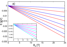
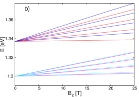
Figure 2: Numerically calculated LL spectrum of WSe₂. a) The first few LL in the higher spin-split VB. Red lines: the $K$ valley ($\tau=1$), blue lines: the $-K$ valley ($\tau=-1$). The inset shows the LLs in the lower spin-split VB. b) The first few LL in the CB. LLs both in lower spin-split band and in the higher spin-split band are shown. Red and purple lines: the $K$ valley, blue and cyan:the $-K$ valley.

Further details of the VDB, including its dependence on the parameter set that can be extracted from DFT calculations, will be discussed in Section 2.2. Here we point out that these results qualitatively agree with the TB calculations of Reference [27, 28, 29], i.e., the continuum approach can reproduce all important features of multi-band TB calculations. A more quantitative comparison between our results and the TB results [27, 28, 29] is difficult, partly because the details may depend on the way how the material parameters are extracted from the DFT band structure and also because in the TB calculations the Zeeman effect was often neglected.

The LL energies can also be obtained analytically in the approximation where $H^{\tau,s}_{3w}$ and $H^{\tau,s}_{cub,1}$ are neglected. We will not show these analytical results here because it turns out that an even simpler approximation yields a good agreement with the numerical calculations shown in Figures 1 and 2 (see Section 2.2) and offers a suitable starting point to develop a theory for the SdH oscillations of the longitudinal conductivity.

2.2 Approximation of the LLs spectrum

In zero magnetic field, the trigonal warping term Eq. (7i) and the third order term Eq. (7l) are important in order to understand the results of recent angle resolved photoelectron spectroscopy measurements and in order to obtain a good fit to the DFT band structure, respectively [3]. However, as we will show for the calculation of LLs the terms $H^{\tau,s}_{3w}$ and $H^{\tau,s}_{cub,1}$ are less important. To see this one can perform another Löwdin-partitioning on $H_{\rm eff}^{\tau,s}$ to obtain effective singe-band Hamiltonians for the VB and the CB separately. Keeping only lowest order terms in $B_{z}$ one finds that these single-band Hamiltonians correspond to a harmonic oscillator Hamiltonian (with different effective masses in the VB and CB and for the spin-split bands) and a term which describes a linear-in-$B_{z}$ splitting of the energies of the LLs in the two valleys. Therefore the LL spectrum can be approximated by

$$E_{n,{\rm vb}}^{\tau,s}=\varepsilon_{\rm vb}^{\tau,s}+\hbar\omega_{{\rm vb}}^{(\tau,s)}\left(n+\frac{1}{2}\right)+\frac{1}{2}g_{e}\mu_{B}B_{z}s+\frac{1}{2}g_{vl,{\rm vb}}^{(s)}\mu_{B}B_{z}\,\tau,$$ (7ha)

$$E_{n,{\rm cb}}^{\tau,s}=\varepsilon_{\rm cb}^{\tau,s}+\hbar\omega_{{\rm cb}}^{(\tau,s)}\left(n+\frac{1}{2}\right)+\frac{1}{2}g_{e}\mu_{B}B_{z}s+\frac{1}{2}g_{vl,{\rm cb}}^{(s)}\mu_{B}B_{z}\,\tau.$$ (7hb)

Here, the following notations are introduced: $n=0,1,2,\dots$ is an integer denoting the LL index, $\varepsilon_{\rm vb(cb)}^{\tau,s}=\varepsilon_{\rm vb(cb)}+\tau\Delta_{\rm vb(cb)}s_{z}$ are the band edge energies in the VB (CB) for a given spin-split band $s$ and $\omega_{{\rm vb\,(cb)}}^{(\tau,s)}=\frac{eB_{z}}{m_{\rm vb\,(cb)}^{(\tau,s)}}$ are cyclotron frequencies. In terms of the parameters appearing in Eqs. (2)-(6), for $\tau=1$ the effective masses $m_{\rm vb\,(cb)}^{(s)}$ that enter the expression of the cyclotron frequencies are given by [3]

$$\frac{\hbar^{2}}{2m_{\rm vb}^{(1,s)}}=\left(\frac{\hbar^{2}}{2m_{e}}+\alpha_{s}-\frac{|\gamma|^{2}}{E_{\rm bg}^{(s)}}\right)$$ (7hia)

$$\frac{\hbar^{2}}{2m_{\rm cb}^{(1,s)}}=\left(\frac{\hbar^{2}}{2m_{e}}+\beta_{s}+\frac{|\gamma|^{2}}{E_{\rm bg}^{(s)}}\right)$$ (7hib)

where ${E_{\rm bg}^{(s)}}=\varepsilon_{\rm cb}^{1,s}-\varepsilon_{\rm vb}^{1,s}$. The corresponding expressions for $\tau=-1$ can be easily found from the requirement electronic states that are connected by time reversal symmetry have the same effective mass. This means that bands corresponding to the same value of the product $\tau\,s$ have the same effective mass. The third term in Eqs (7ha) and (7hb) comes from the free-electron term (2). The VDB is described by the last term in Eqs. (7ha), (7hb) and the valley g-factors are given by

$$g_{vl,{\rm vb}}^{(s)}=4\frac{m_{e}}{\hbar^{2}}\left(\alpha_{s}+\frac{|\gamma|^{2}}{E_{bg}^{(s)}}\right)$$ (7hija)

$$g_{vl,{\rm cb}}^{(s)}=4\frac{m_{e}}{\hbar^{2}}\left(\frac{|\gamma|^{2}}{E_{bg}^{(s)}}-\beta_{s}\right).$$ (7hijb)

As one can see from (7hija)-(7hijb), $g_{vl}^{(s)}$ depends on the (virtual) inter-band transition matrix elements $\alpha_{s}$, $\beta_{s}$ and $\gamma$. Due to the intrinsic spin-orbit coupling, the magnitude of these matrix elements is spin-dependent [3]. Note, that $g_{vl}$ is different in the VB and the CB. This is in agreement with numerical calculations based on multi-band tight-binding models [27, 29]. For the CB, the details of the derivation that leads to (7hb) can be found in [34], for the VB the derivation of (7ha) is analogous and therefore it will not be detailed here. We note that in variance to Reference [34], we do not define separately an out-of-plane spin g-factor and a spin independent valley g-factor, these two g-factors are merged in $g_{vl}^{(s)}$. The response to magnetic field also depends on the free electron Zeeman term. The spin-index $s$ to be used in the evaluation of the Zeeman term in Eqs. (7ha)-(7hb) follows the spin-polarization of the given spin-split band. For MoS₂, the spin polarizations $s$ of each band are shown in Figure 5, other MoX₂ (X={S, Se, Te}) monolayer TMDCs have the same polarization. For monolayer WX₂ TMDCs the spin polarization in the VB is the same as for the MoX₂, but in the CB the polarization of the lower (higher) spin-split band is the opposite [3]. We are mainly interested in how the magnetic field breaks the degeneracy of those electronic states which are connected by time reversal in the absence of the magnetic field. Using Eqs. (7ha)-(7hb), the valley splitting $\delta E_{\rm cb(vb)}^{(i)}=g^{(i)}_{eff,{\rm cb\,(vb)}}\mu_{B}B_{z}$ of these states can be characterized by an effective g-factor $g^{(i)}_{eff,{\rm cb\,(vb)}}=(g_{e}s\tau+g_{vl,{\rm cb\,(vb)}}^{(s)})$, where $i=1(2)$ denotes the higher-in-energy (lower-in-energy) spin-split band. In the VB the upper index ${(1)}$ [${(2)}$] is equivalent to $\downarrow$ ($\uparrow$), but in the CB the relation depends on the specific material being considered because the polarisation is different for MoX₂ and WX₂ materials. Taking first the MoX₂ monolayers one finds that (see also Figure 5)

$$g^{(1)}_{eff,{\rm vb}}=(-g_{e}+g_{vl,{\rm vb}}^{\downarrow})\hskip 28.45274ptg^{(2)}_{eff,{\rm vb}}=(g_{e}+g_{vl,{\rm vb}}^{\uparrow})$$ (7hijka)

$$g^{(1)}_{eff,{\rm cb}}=(g_{e}+g_{vl,{\rm cb}}^{\uparrow})\hskip 28.45274ptg^{(2)}_{eff,{\rm cb}}=(-g_{e}+g_{vl,{\rm cb}}^{\downarrow})$$ (7hijkb)

For WX₂ monolayers $g^{(i)}_{eff,{\rm vb}}$ can also be calculated by (7hijka), whereas in the CB

$$g^{(1)}_{eff,{\rm cb}}=(-g_{e}+g_{vl,{\rm cb}}^{\downarrow})\hskip 28.45274ptg^{(2)}_{eff,{\rm cb}}=(g_{e}+g_{vl,{\rm cb}}^{\uparrow})$$ (7hijkl)

As an example the numerical values of the various g-factors defined above are given in Table 1 for MoS₂ and in Table 2 for WSe₂. One can see that $g_{vl,{\rm cb\,(vb)}}^{(s)}$ can be comparable in magnitude to $g_{e}$. This explains why the valley splitting is very small for MoS₂ in the case of the upper spin-split band in the CB (see Figure 1), whereas the opposite is true for WSe₂ (Figure 2).

As one can see from Eqs. (7hija) and (7hijb), $g_{vl}^{(s)}$ depends explicitly on the band-gap $E_{bg}^{(s)}$ of a given spin $s$. In addition, the parameters $\gamma$, $\alpha_{s}$ and $\beta_{s}$ implicitly also depend on $E_{bg}^{(s)}$ due to the fitting procedure that is used to obtain them from DFT band structure calculations[3]. It is known that $E_{bg}^{(s)}$ is underestimated in DFT calculations and its exact value at the moment is not known for most monolayer TMDCs. Therefore in Reference [3] we have obtained two sets of the $\mathbf{k}\cdot\mathbf{p}$ band structure parameters, the first one using $E_{bg}^{(s)}$ from DFT and the second one using $E_{bg}^{(s)}$ extracted from GW calculations. The calculations shown in Figures 1 and 2 were obtained with the former parameter set. As shown in Table 1, the calculated g-factors depend quite significantly on the choice of the parameter set. While there is an uncertainty regarding the magnitude of $g_{vl}^{(s)}$, we expect that the g-factors obtained by using the DFT and the GW parameter sets will bracket the actual experimental values. On the other hand, the effective masses are probably captured quite well by DFT calculations and therefore the first term in Eqs. (7ha)-(7hb) is less affected by the uncertainties of the band structure parameters. The calculations in Figures 1 and 2 correspond to the “DFT” parameter set in Tables 1 and 2.

Table 1: Valley g-factors in MoS₂. In the first row the g-factors are obtained with the help of DFT band gap, in the second row the g-factors are calculated with a band gap taken from the $GW$ calculations.

• 	$E_{\rm bg}^{\downarrow}$	$E_{\rm bg}^{\rm\uparrow}$	$g_{vl,{\rm vb}}^{\downarrow}$	$g_{vl,{\rm vb}}^{\uparrow}$	$g_{eff,\rm{vb}}^{(1)}$	$g_{eff,\rm{vb}}^{(2)}$	$g_{vl,{\rm cb}}^{\downarrow}$	$g_{vl,{\rm cb}}^{\uparrow}$	$g_{eff,\rm{cb}}^{(1)}$	$g_{eff,\rm{cb}}^{(2)}$
  DFT	$1.66\,{\rm eV}^{a}$	$1.838\,{\rm eV}^{a}$	$0.98$	$0.96$	$-1.02$	$2.96$	$-2.11$	$-2.05$	$-0.05$	$-4.11$
  GW	$2.8\,{\rm eV}^{b}$	$2.978\,{\rm eV}^{b}$	$2.57$	$2.38$	$0.57$	$4.38$	$-0.52$	$-0.6$	$1.4$	$-2.52$

• ^a adapted from Reference [3].

• ^b adapted from Reference [35].

Table 2: Valley g-factors in WSe₂. In the first row the g-factors are obtained with the help of DFT band gap, in the second row the g-factors are calculated with a band gap taken from the $GW$ calculations.

• 	$E_{\rm bg}^{\downarrow}$	$E_{\rm bg}^{\rm\uparrow}$	$g_{vl,{\rm vb}}^{\downarrow}$	$g_{vl,{\rm vb}}^{\uparrow}$	$g_{eff,\rm{vb}}^{(1)}$	$g_{eff,\rm{vb}}^{(2)}$	$g_{vl,{\rm cb}}^{\downarrow}$	$g_{vl,{\rm cb}}^{\uparrow}$	$g_{eff,\rm{cb}}^{(1)}$	$g_{eff,\rm{cb}}^{(2)}$
  DFT	$1.337{\rm eV}^{a}$	$1.766{\rm eV}^{a}$	$-0.38$	$-0.23$	$-2.38$	$1.77$	$-2.71$	$-2.81$	$-4.71$	$-0.81$
  GW	$2.457{\rm eV}^{b}$	$2.886{\rm eV}^{b}$	$2.55$	$1.9$	$0.55$	$3.9$	$-0.67$	$0.13$	$-2.67$	$2.13$

• ^a adapted from Reference [3].

• ^b adapted from Reference [36].

In order to see the accuracy of the approximation introduced in Eq. (7hia)-(7hib), in Figure 3 we compare the LL spectrum obtained in this approximation and calculated numerically using the Hamiltonian (1). As one can see the approximation is very good both in the VB and in the CB up to magnetic fields $\lesssim 20{\rm T}$. For larger magnetic fields and large LL indices ($n>7$) deviations start to appear between the full quantum results and the approximation. The deviations are stronger in the VB which we attribute to the larger trigonal warping [3] of the band structure in the VB. To our knowledge the effects of the non-parabolicity of the band-dispersion on the LL spectrum has not been discussed before for monolayer TMDCs.

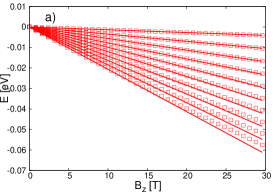
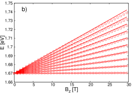
Figure 3: Comparison of the LL spectrum in MoS₂ obtained from the two-band model and from the single band model. a) The numerically calculated LLs using (1) for the $\tau=1$, $s=-1$ in the VB (squares) and the approximation (7ha) (solid lines) for LL indices $n=0\dots 9$. b) the same as in a) but for the for the $\tau=1$, $s=-1$ band in the CB (squares) and the approximation (7hb) (solid lines).

Given the noticeable uncertainty regarding the exact values of the effective g-factors, one may ask which features of the LL spectrum are affected or remain qualitatively the same. Looking at Tables 1 and 2, one can see that in some cases only the magnitude of an effective g-factor changes, in other cases both the magnitude and the sign. Firstly, we consider a case which illustrates possible effects of the uncertainty in the magnitude of an effective g-factor.

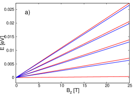
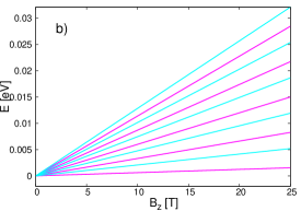
Figure 4: Comparison of the LL spectrum in in the lower-in-energy spin-split CB of MoS₂ obtained with a) $g_{eff,{\rm cb}}^{(2)}=-4.11$ and b) $g_{eff,{\rm cb}}^{(2)}=-2.52$. LLs in different valleys are denoted by different colors.

In Figure 4 we show the LLs in the lower spin-split CB in MoS₂ for the two different $g_{eff,{\rm cb}}^{(2)}$ given in Table 1. One can see that in Figure 4(a) the VDB is small, except for the lowest LL, which is clearly separated from the other LLs. If one assumes that the LLs acquire a finite broadening then all LLs would appear as doubly degenerate except the lowest one in, e.g. an STM measurement. In contrast, the LLs are in Figure 4(b) are more evenly spaced and may appear as non-degenerate even if they are broadened.

Secondly, in some cases also the sign of $g_{eff}$ changes depending on which parameter set is used. For $g_{eff}>0$ the LLs in the $K$ valley have higher energy than the LLs in the $-K$ valley, while for negative $g_{eff}$ the opposite is true. We note that in Reference[37] Eqs (7ha)-(7hb) were used to understand the VDB in the excitonic transitions in MoSe₂. The exciton valley g-factor $g_{vl,exc}$ was obtained by considering the energy difference between the lowermost LL in the CB and the uppermost LL in the VB in each valley:

$$g_{ex,vl}\mu_{B}B_{z}=(E_{n=0,{\rm cb}}^{\tau=1,\downarrow}-E_{n=0,{\rm vb}}^{\tau=1,\downarrow})-(E_{n=0,{\rm cb}}^{\tau=-1,\uparrow}-E_{n=0,{\rm vb}}^{\tau=-1,\uparrow}).$$ (7hijkm)

Using Eqs. (7hia)-(7hijb), one can easily show that in this approximation the exciton valley g-factor is independent of the band gap and it can be expressed in terms of the effective masses in the CB and VB [37, 38]:

$$g_{ex,vl}=4-2\left(\frac{m_{e}}{m_{cb}^{s}}-\frac{m_{e}}{|m_{vb}^{s}|}\right)$$ (7hijkn)

Therefore, albeit the effective g-factors in the CB and VB separately are affected by uncertainties, the exciton g-factor, in principle, can be calculated more precisely so long the effective masses are captured accurately by DFT calculations. The comparison of DFT results and ARPES measurements [3] suggest that the DFT effective masses in the VB match the experimental results quite well. At the moment, however, it is unclear how accurate are the DFT effective masses in the CB.

Finally, we make the following brief comments.

• In the gapped-graphene approximation, i.e., if one neglects the free electron term and the terms $\sim\alpha_{s},\beta_{s}$ in Eqs. (7hia)-(7hib) and in (7hija)-(7hijb) then the lowest LL in the CB and the highest one in the VB will be non-degenerate, but for all other LLs the valley degeneracy would not be lifted [31] due to a cancellation effect between the first and last terms in Eqs.(7ha) and (7hb).

• By measuring the valley g-factors and the effective masses one can deduce the Diracness of the spectrum [48], i.e., the relative importance of the off-diagonal and diagonal terms in $H^{\tau,s}_{D}$ (7c) and $H^{\tau,s}_{\rm as}$ (7f), respectively.

3 Shubnikov-de Haas oscillations of longitudinal conductivity

As we will show, the results of the Section 2.2 provide a convenient starting point for the calculation of the SdH oscillations of the magnetoconductance. Our main motivation to consider this problem comes from the recent experimental observation of SdH oscillations in monolayer [18] and few-layer [18, 20] samples. Regarding previous theoretical works on magnetotransport in TMDCs, quantum corrections to the low-field magneto-conductance were studied in References [25, 26]. A different approach, namely, the Adams-Holstein cyclotron-orbit migration theory [39], was used in Reference [40] to calculate the longitudinal magnetoconductance $\sigma_{xx}$. This theory is applicable if the cyclotron frequency is much larger than the average scattering rate $1/\bar{\tau}_{sc}$. By using the effective mass obtained from DFT calculations [3] and taking the measured values of the zero field electron mobility $\mu_{e}=\frac{e^{2}n_{e}\bar{\tau}_{sc}}{m_{cb}}$ and the electron density $n_{e}$ given in Reference [18] for monolayer MoS₂, a rough estimate for $\bar{\tau}_{sc}$ can be obtained. This shows that for magnetic fields $B\lesssim 15\,$T the samples are in the limit of $\omega_{cb}\bar{\tau}_{sc}\lesssim 1$ and therefore the Adams-Holstein approach cannot be used to describe $\sigma_{xx}$. Therefore we will extend the approach of Ando [42] to calculate $\sigma_{xx}$ in monolayer TMDCs because it can offer a more direct comparison to existing experimental results.

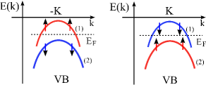
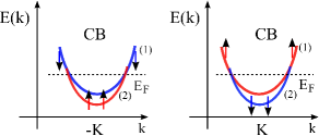
Figure 5: Schematics of the dispersion in the VB and in the CB around the $K$ and $-K$ points of the band structure. The spin-split bands are denoted by red and blue lines, different colours indicate different spin-polarization. The arrows show the spin-polarization for MoS₂. For typical values of doping, the Fermi-level $E_{F}$ (denoted by a dashed line) would intersect only the upper spin-split band in the VB or both spin-split bands in the CB. The index $(1)$ and $(2)$ denote the upper and lower spin-split band.

Before presenting the detailed theory of SdH oscillations we qualitatively discuss the role of the doping and the assumptions that we will use. The most likely scenarios in the VB and the CB are shown in Figure 5 (a) and (b), respectively. Considering first the CB, for electron densities $n_{e}\sim 10^{13}/{\rm cm^{2}}$ measured in Reference [18] both the upper and lower spin-split bands would be occupied. In contrast, due to the much larger spin-splitting, for hole doped samples $E_{F}$ would typically intersect only the upper spin-split VB. Such a situation may also occur for n-doped samples in those monolayer TMDCs where the spin-splitting in the CB is much larger than in MoS₂, e.g., in MoTe₂ or WSe₂. For strong doping other extrema in the VB and CB, such as the $\Gamma$ and $Q$ points may also play a role, this will be briefly discussed at the end of this section.

We will have two main assumptions in the following. The first one is that one can neglect inter-valley scattering and also intra-valley scattering between the spin-split bands. Clearly, this is a simplified model whose validity needs to be checked against experiments. One can argue that in the VB (see Figure 5(a)) in the absence of magnetic impurities the inter-valley scattering should be strongly suppressed because it would also require a simultaneous spin-flip. A recent scanning-tunneling experiment in monolayer WSe₂ [41] indeed seems to show a strong supression of inter-valley scattering. In the CB, for the case shown in Figure 5(b), the inter-valley scattering is not forbidden by spin selection rules. Even if $E_{F}$ was smaller, such that only one of the spin-split bands is populated in a given valley, the inter-valley scattering would not be completely suppressed because the bands are broadened by disorder which can be comparable to the spin-splitting $2\Delta_{cb}$ ($2\Delta_{cb}=3\,$meV for MoS₂ and $20-30\,$meV for other monolayer TMDCs.) On the other hand, the intra-valley scattering between the spin-split bands in the CB should be absent due to the specific form of the intrinsic SOC, see Eq. (5). We note that strictly speaking any type of perturbation which breaks the mirror symmetry of the lattice, such as a substrate or certain type of point defects (e.g., sulphur vacancies) would (locally) lead to a Rashba type SOC and hence induce intra-valley coupling between the spin-split bands. It is not known how effective is this mechanism, in the present study we neglect it. The second assumption is that we only consider the effect of short range scatterers. This assumption is widely used in the interpretation of SdH oscillations as it facilitates to obtain analytical results [42]. We note that according to References [18, 24], some evidence for the presence of short range scatterers in monolayer MoS₂ has indeed been recently found. While short-range scatterers can, in general, cause inter-valley scattering, on the merit of its simplicity as a minimal model we only take into account intra-valley intra-band scattering.

Using these assumptions it is straightforward to extend the theory of Ando [42] to the SdH oscillations of monolayer TMDCs. Namely, as it has been shown in Section 2.2, for not too large magnetic fields the LLs in a given band can be described by a formula which is the same as for a simple parabolic band except that it contains a term which describes a linear-in-magnetic field valley-splitting. Then, because of the assumption that one can neglect inter-valley and intra-valley inter-band scattering, the total conductance will be the sum of the conductances of individual bands with valley and spin indices $\tau,s$. This simple model allows us to focus on the effects of intrinsic SOC and valley splitting on the SdH oscillations, which is our main interest here.

Following Reference [42], we treat impurity scattering in the self-consistent Born approximation (SCBA) and use the Kubo-formalism to calculate the longitudinal conductivity $\sigma_{xx}$ (for a recent discussion see, e.g., [43, 44]). Assuming a random disorder potential $V(\mathbf{r})$ with short range correlations $\langle V(\mathbf{r})V(\mathbf{r}^{\prime})\rangle=\lambda_{sc}\delta(\mathbf{r}-\mathbf{r}^{\prime})$, the self-energy $\Sigma^{\tau,s}_{R}=\Sigma^{\tau,s}_{r}+i\Sigma^{\tau,s}_{i}$ in a given band ($\tau,s$) does not depend on the LL index $n$. It is given by the implicit equation

$$\Sigma^{\tau,s}_{r}+i\Sigma^{\tau,s}_{i}=\frac{\lambda_{sc}}{2\pi l_{B}^{2}}\sum_{n=0}^{\infty}\frac{1}{E-E_{n}^{\tau,s}-(\Sigma^{\tau,s}_{r}+i\Sigma^{\tau,s}_{i})}$$ (7hijko)

where $E_{n}^{\tau,s}$ is given by Eqs (7ha)-(7hb). The term $\lambda_{sc}/2\pi l_{B}^{2}$ on the right-hand side of Eq.(7hijko) can be rewritten as $\frac{\lambda_{sc}}{2\pi l_{B}^{2}}=\frac{1}{2\pi}\hbar\omega_{c}^{(i)}\frac{\hbar}{\tau_{sc}^{(i)}}$ where $1/\tau_{sc}^{(i)}=\lambda_{sc}m^{(i)}/\hbar^{3}$ is the scattering rate calculated in the Born-approximation in zero magnetic field. As in Section 2.2, the upper index $i=1(2)$ refers to the higher(lower)-in-energy spin-split band in a given valley (see also Figure 5). Using the Kubo-formalism the conductivity coming from a single valley and band $\sigma_{xx}^{\tau,s}$ is calculated as

$$\sigma_{xx}^{\tau,s}=\frac{e^{2}}{\pi^{2}\hbar}\int\mathnormal{d}E\left(-\frac{\partial f(E)}{\partial E}\right)\sigma_{xx}^{\tau,s}(E)$$ (7hijkp)

where $f(E)$ is the Fermi function and

$$\sigma_{xx}^{\tau,s}(E)=(\hbar\omega_{c}^{(i)})^{2}\sum_{n=0}^{\infty}(n+1){\rm Re}[ G^{\tau,s}_{A}(n,E)G^{\tau,s}_{R}(n+1,E)- G^{\tau,s}_{A}(n,E)G^{\tau,s}_{A}(n+1,E)].$$ (7hijkq)

Here $G^{\tau,s}_{R}(n,E)$ and $G^{\tau,s}_{A}(n,E)$ are the retarded and advanced Greens-functions, respectively. Vertex corrections are neglected in this approximation. Since we neglect inter-valley and intra-valley inter-band scattering, the disorder-averaged Greens-function $G^{\tau,s}_{R,A}(n,E)=[E-E_{n}^{\tau,s}-\Sigma^{\tau,s}_{R,A}]^{-1}$ is diagonal in the indices $\tau,s$ and in the LL representation it is also diagonal in the LL index $n$. The total conductivity is then given by $\sigma_{xx}=\sum_{\tau,s}\sigma_{xx}^{\tau,s}$ where the summation runs over occupied subbands for a given total electron (hole) density $n_{e}$ ($n_{h}$). In general, one has to determine $\Sigma^{\tau,s}_{r}+i\Sigma^{\tau,s}_{i}$ by soving Eq. (7hijko) numerically. The Greens-functions $G^{\tau,s}_{R,A}$ can be then calculated and $\sigma_{xx}^{\tau,s}$ follows from Eq. (7hijkq). It can be seen from Eq. (7hijkp) that at zero temperature $\Sigma^{\tau,s}(E)$ and $\sigma_{xx}^{\tau,s}(E)$ has to be evaluated at $E=E_{F}$. In the semiclassical limit, when there are many occupied LLs below $E_{F}$, i.e., $\hbar\omega^{(i)}_{c}\ll E_{F}$, one can derive an analytical result for $\sigma_{xx}^{\tau,s}$, see References [42, 43] for the details of this calculation. Here we only give the final form of $\sigma_{xx}$ and compare it to the results of numerical calculations.

As mentioned above, the situation depicted in Figure 5(a), i.e., when there is only one occupied subband in each of the valleys is probably most relevant for p-doped samples. One finds that in this case the longitudinal conductance is

$$\sigma_{xx}/\sigma_{0}=\frac{2}{1+(\omega_{\rm vb}^{(1)}\tau_{sc}^{(1)})^{2}}\left[1-\frac{4(\omega_{\rm vb}^{(1)}\tau_{sc}^{(1)})^{2}}{1+(\omega_{\rm vb}^{(1)}\tau_{sc}^{(1)})^{2}}e^{-\frac{\pi}{(\omega_{\rm vb}^{(1)}\tau_{sc}^{(1)})}}\cos\left(\frac{2\pi E_{F}}{\hbar\omega_{\rm vb}^{(1)}}\right)\mathcal{A}_{1}\,\mathcal{B}\right.$$

$$+\left.\frac{g_{eff}^{(i)}}{2}\frac{\mu_{B}B_{z}}{E_{F}}\frac{4(\omega_{\rm vb}^{(1)}\tau_{sc}^{(1)})^{2}}{1+(\omega_{\rm vb}^{(1)}\tau_{sc}^{(1)})^{2}}e^{-\frac{\pi}{(\omega_{\rm vb}^{(1)}\tau_{sc}^{(1)})}}\sin\left(\frac{2\pi E_{F}}{\hbar\omega_{\rm vb}^{(1)}}\right)\mathcal{A}_{2}\,\mathcal{B}\right].$$ (7hijkr)

Here $\sigma_{0}=\frac{e^{2}\tau_{sc}^{(1)}}{2\pi\hbar^{2}}E_{F}=\frac{e^{2}\tau_{sc}^{(1)}}{m_{\rm vb}^{(1)}}\frac{n_{h}}{2}$ is the zero field conductivity per single valley and band, $n_{h}$ is the total charge density and we assumed $\Sigma^{\tau,s}_{r}\ll\Sigma^{\tau,s}_{i}\ll E_{F}$. The amplitudes $\mathcal{A}_{1,2}$ and $\mathcal{B}$ are given by

$$\mathcal{A}_{1}=\cos\left(\frac{\pi}{2}g_{eff,{\rm vb}}^{(1)}\frac{m_{\rm vb}^{(1)}}{m_{e}}\right),\hskip 28.45274pt\mathcal{A}_{2}=\sin\left(\frac{\pi}{2}g_{eff,{\rm vb}}^{(1)}\frac{m_{\rm vb}^{(1)}}{m_{e}}\right);$$ (7hijksa)

$$\mathcal{B}=\frac{2\pi^{2}k_{B}T/\hbar\omega_{\rm vb}^{(1)}}{\sinh\left({2\pi^{2}k_{B}T/\hbar\omega_{\rm vb}^{(1)}}\right)},$$ (7hijksb)

where $k_{B}$ is the Boltzmann constant and $T$ is the temperature. One can see that Eqs. (7hijkr)-(7hijksb) are very similar to the well known expression derived by Ando [42] for a two-dimensional electron gas (2DEG). The valley-splitting, which leads to the appearance of the amplitudes $\mathcal{A}_{1,2}$, plays an analogous role to the Zeeman spin-splitting in 2DEG. Therefore, under the assumption we made above, the uncertainty regarding the value of the effective g-factors affects the amplitude of the oscillations but not their phase. The term proportional to $\mu_{B}B_{z}/E_{F}$ in Eq. (7hijkr) is usually much smaller than the first term. Thus, it can be neglected in the calculation of the total conductance, but may be important if one is interested only in the oscillatory part of $\sigma_{xx}$, see below.

We emphasize that Eq. (7hijkr) is only accurate if $\hbar\omega_{\rm vb}^{(1)}\ll E_{F}$. However, in semiconductors, especially at relatively low doping, one can reach magnetic field values where the cyclotron energy becomes comparable to $E_{F}$. In this case the numerically calculated $\sigma_{xx}$ may differ from Eq. (7hijkr) . It is known that, e.g., WSe₂ can be relatively easily gated into the VB, and a decent Hall mobility was recently demonstrated in few-layer samples in Reference [15]. As a concrete example we take the following values [15]: $n_{h}=-4*10^{12}/cm^{2}$ and Hall mobility $\mu_{H}=700cm^{2}/Vs$. By taking $m_{vb}^{(1)}=-0.36m_{e}$ [3] the Fermi energy is $E_{F}\approx-26.6$meV and using that $\mu_{H}=e\tau_{sc}^{(1)}/m^{(1)}_{vb}$ we obtain $\tau_{sc}^{(1)}=1.4\times 10^{-13}$s. The amplitude of the oscillations should become discernible when $\omega_{vb}^{(1)}\tau_{sc}^{(1)}=\mu_{H}B_{z}\lesssim 1$, i.e., for magnetic fields $B_{z}\gtrsim 10$T, while at $B_{z}=14.28$T, which corresponds to $\omega_{vb}^{(1)}\tau_{sc}^{(1)}\approx 1$, there are around six occupied LLs. One can expect that for $B_{z}\lesssim 15\,$T the LL spectrum is well described by Eq(7ha), however, since the number of LLs is relatively low, there might be deviations between the analytically and numerically calculated $\sigma_{xx}$. In Figure 6(a) we show a comparison between the analytical result Eq. (7hijkr) and the numerically calculated longitudinal conductance at zero temperature. The effective g-factors $g_{eff,{\rm vb}}^{(1)}$ used in these calculations are given in Table 2.

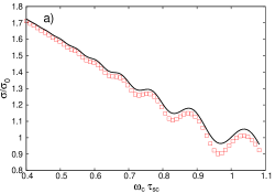
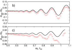
Figure 6: Comparison of the numerically (symbols) and analytically (solid line) calculated zero temperature conductivity for WSe₂ for the situation depicted in Figure 5. a) total conductivity, $g_{eff,{\rm vb}}^{(1)}=0.55$. b) and c) comparison of the oscillatory parts of $\sigma_{xx}$. In b) $g_{eff,{\rm vb}}^{(1)}=0.55$, while in c) $g_{eff,{\rm vb}}^{(1)}=-2.38$ (see Table 2). The figures correspond to a magnetic field range of about $5.7-15.7\,$T.

One can see that for larger magnetic fields the amplitude of the oscillations is not captured very precisely by Eq. (7hijkr) but the overall agreement with the numerical results is good. Next, in Figures 6(b) and (c) we compare the oscillatory parts $\sigma_{xx,osc}$ of the longitudinal conductivity obtained from numerical calculations and from Eq (7hijkr) using two different $g_{eff,{\rm vb}}$ values. In the case of the numerical calculations $\sigma_{xx,osc}$ was obtained by subtracting the smooth function $2/(1+(\omega_{\rm vb}^{(1)}\tau_{sc}^{(1)})^{2})$ from $\sigma_{xx}$. According to Eq. (7hijkr), the valley-splitting of the LLs and the different effective g-factors should only affect the amplitude of the oscillations. While the amplitude of the oscillations indeed depends on $g_{eff,{\rm vb}}^{(1)}$, one can see that the agreement is better for $g_{eff,{\rm vb}}^{(1)}=0.55$ than for $g_{eff,{\rm vb}}^{(1)}=-2.38$. For the latter case the position of the conductance minimuma start to differ for large magnetic field, whereas the maximuma in $\sigma_{xx}$ agree in both figures. These calculations illustrate that Eq. (7hijkr) may not agree with the numerical results when there are only a few LLs below $E_{F}$.

We now turn to the case shown in Figure 5(b) when both spin-split subbands are populated. The total conductance is given by the sum of the conductances coming from the two spin-split subbands : $\sigma_{xx}=\sigma_{xx}^{(1)}+\sigma_{xx}^{(2)}$. Since the effective masses in the spin-split bands are, in general, different, the associated scattering times $\tau_{sc}^{(1)}$ and $\tau_{sc}^{(2)}$ calculated in the Born-approximation are also different. We define $\tilde{\tau}_{sc}=\tau_{sc}^{(1)}+\tau_{sc}^{(2)}$ and $\tilde{\sigma}_{0}=\frac{e^{2}\tilde{\tau}_{sc}}{2\pi\hbar^{2}}E_{F}$, and obtain for the magnetoconductance

$$\sigma_{xx}/\tilde{\sigma}_{0}=2\mathcal{C}^{(2)}\frac{1}{1+(\omega_{\rm cb}^{(2)}\tau_{sc}^{(2)})^{2}}\left[1-\frac{4(\omega_{\rm cb}^{(2)}\tau_{sc}^{(2)})^{2}}{1+(\omega_{\rm cb}^{(2)}\tau_{sc}^{(2)})^{2}}e^{-\frac{\pi}{(\omega_{\rm cb}^{(2)}\tau_{sc}^{(2)})}}\cos\left(\frac{2\pi E_{F}}{\hbar\omega_{\rm cb}^{(2)}}\right)\mathcal{A}_{1}^{(2)}\,\mathcal{B}^{(2)}\right]$$

$$+2\mathcal{C}^{(1)}\frac{1}{1+(\omega_{\rm cb}^{(1)}\tau_{sc}^{(1)})^{2}}\left[1-\frac{4(\omega_{\rm cb}^{(1)}\tau_{sc}^{(1)})^{2}}{1+(\omega_{\rm cb}^{(1)}\tau_{sc}^{(1)})^{2}}e^{-\frac{\pi}{(\omega_{\rm cb}^{(1)}\tau_{sc}^{(1)})}}\cos\left(\frac{2\pi(E_{F}-2\Delta_{cb})}{\hbar\omega_{\rm cb}^{(1)}}\right)\mathcal{A}_{1}^{(1)}\,\mathcal{B}^{(1)}\right]$$ (7hijkst)

Here

$$\mathcal{C}^{(1)}=\left(1-\frac{2\Delta_{cb}}{E_{F}}\right)\frac{\tau_{sc}^{(1)}}{\tilde{\tau}_{sc}},\hskip 28.45274pt\mathcal{C}^{(2)}=\frac{\tau_{sc}^{(2)}}{\tilde{\tau}_{sc}},$$ (7hijksua)

$$\mathcal{A}_{1}^{(i)}=\cos\left(\frac{\pi}{2}g_{eff}^{(i)}\frac{m_{{\rm cb}}^{(i)}}{m_{e}}\right),$$ (7hijksub)

$$\mathcal{B}^{(i)}=\frac{2\pi^{2}k_{B}T/\hbar\omega_{\rm cb}^{(i)}}{\sinh\left({2\pi^{2}k_{B}T/\hbar\omega_{\rm cb}^{(i)}}\right)}.$$ (7hijksuc)

In Eq. (7hijkst) we have neglected terms which are $\sim\mu_{B}B_{z}/E_{F}$. The result shown in Eq. (7hijkst) is similar to the multiple subband occupation problem in 2DEG [45, 46, 47]. The valley splitting affects the amplitude of the oscillations (see Eq. (7hijksub)), whereas the intrinsic SOC can influence the amplitude of the oscillations [see Eq. (7hijksua)] and it also leads to a phase difference [Eq. (7hijkst)] between the oscillations coming from the two spin-split subbands.

The situation depicted in Figure 5(b) is easily attained, e.g., in the CB of monolayer MoS₂, where DFT calculations predict that the spin-splitting is $2\Delta_{cb}=3$ meV and therefore both subbands can be populated for relatively low densities. Our choice of the parameters for the numerical calculations shown below is motivated by the recent experiment of Cui et al. [18], where SdH oscillations in mono- and few layer MoS₂ samples have been measured. We use $n_{e}=10^{13}/cm^{2}$ and mobility $\mu_{H}=1000{\rm cm^{2}/Vs}$. The effective masses are chosen as $m_{cb}^{(1)}=0.46m_{e}$, $m_{cb}^{(2)}=0.43m_{e}$ and the spin-splitting in the CB is $2\Delta_{cb}=3$ meV [3]. Using these parameters we find $E_{F}=28.43$ meV. Since the effective masses are rather similar, the scattering times calculated from $\mu_{H}$ are close to each other: $\tau_{sc}^{(1)}\approx\tau_{sc}^{(2)}\approx 2.6\times 10^{-13}$s, i.e., they are almost twice as long as in the case of WSe₂. The oscillations in $\sigma_{xx}$ should become discernible for $B_{z}\gtrsim 7\,$T, and at $B_{z}=10$T there are ten LLs in both the lower and the upper spin-split CB in each valley. We will focus on the oscillatory part $\sigma_{xx,osc}=\sigma_{xx,osc}^{(1)}+\sigma_{xx,osc}^{(2)}$ of the conductance, since this contains information about the spin and valley splittings. As in the previous example, we first calculate $\sigma_{xx}^{(i)}$ numerically using Eqs. (7hijko)-(7hijkq) and obtain $\sigma_{xx,osc}^{(i)}$ by subtracting the smooth function $2\mathcal{C}^{(i)}/[1+(\omega^{(i)}_{c}\tau_{sc}^{(i)})^{2}]$. We than compare these results to the oscillations that can be obtained from Eq. (7hijkst).

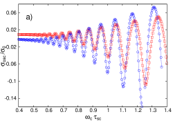
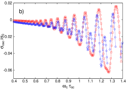
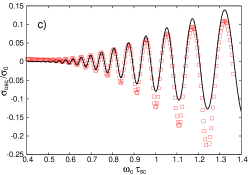
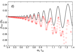
Figure 7: Oscillations of $\sigma_{xx}$ in n-doped MoS₂. a) numerically calculated $\sigma_{osc}^{(1)}$ (red squares) and $\sigma_{osc}^{(2)}$ (blue circles) using $g_{eff,{\rm cb}}^{(1)}=-0.05$ and $g_{eff,{\rm cb}}^{(2)}=-4.11$. b) numerically calculated $\sigma_{osc}^{(1)}$ (red squares) and $\sigma_{osc}^{(2)}$ (blue circles) using $g_{eff,{\rm cb}}^{(1)}=1.44$ and $g_{eff,{\rm cb}}^{(2)}=-2.55$. c) The total oscillatory conductance $\sigma_{osc}=\sigma_{osc}^{(1)}+\sigma_{osc}^{(2)}$ corresponding to a) (red squares) and the analytical result calculated from Eq. (7hijkst) (solid line). d) the same as in c) but corresponding to b).The figures correspond to a magnetic field range of about $4-14\,$T.

In Figures 7(a) and (b) we show the numerically calculated $\sigma_{xx}^{(1)}$ and $\sigma_{xx}^{(2)}$ for the two different sets of g-factor values given in Table 1 as a function of $\bar{\omega}_{c}\bar{\tau}_{sc}$ which was introduced as a dimensionless scale of the magnetic field. Here $\bar{\omega_{c}}=\frac{eB_{z}}{\bar{m}_{cb}}$ with $\bar{m}=\sqrt{m_{cb}^{(1)}m_{cb}^{(2)}}$ and $\bar{\tau}_{sc}=\sqrt{\tau_{sc}^{(1)}\tau_{sc}^{(2)}}$. All calculations are at zero temperature. One can observe that due to the CB spin splitting $2\Delta_{cb}$ the oscillations of $\sigma_{xx}^{(1)}$ and $\sigma_{xx}^{(2)}$ will not be in-phase for larger magnetic field. This effect is expected to be even more important for TMDCs having larger $2\Delta_{cb}$ than MoS₂ and leads to more complex oscillatory features in the total conductance $\sigma_{xx}$ than in the previous example of p-doped WSe₂ where only one band in each valley contributed to the conductance. One can also observe that in Figure 7(b) additional peaks with smaller amplitude appear in $\sigma_{xx,osc}^{(2)}$ for larger magnetic fields, while there are no such peaks in $\sigma_{xx,osc}^{(2)}$ in Figure 7(a). The origin of this behaviour can be traced back to the different valley-splitting patterns shown in Figure 4. The valley splitting of the LLs in Figure 4(a) is small (except for the lowest LL), while in Figure 4(b) all LLs belonging to different valleys are well-separated for larger fields and this leads to the appearance of the additional, smaller amplitude peaks in $\sigma_{xx,osc}^{(2)}$ in Figure 7(b). The comparison between the numerically calculated total oscillatory part $\sigma_{xx,osc}=\sigma_{xx,osc}^{(1)}+\sigma_{xx,osc}^{(2)}$ and the corresponding analytical result given in Eq. (7hijkst) is shown in Figures 7(c) and (d). The agreement between the two approaches is qualitatively good for $\bar{\omega}_{c}\bar{\tau}_{sc}\lesssim 1$. However, for larger magnetic fields where $\bar{\omega}_{c}\bar{\tau}_{sc}\gtrsim 1$ the amplitude of the oscillations start to differ. In this regime the oscillatory behaviour in $\sigma_{xx,osc}$ can be quite complex, influenced by both the valley splitting and also by the intrinsic SOC splitting of the bands.

We have tried to analyze the experimental results by Cui et al. [18] using the theoretical approach outlined above. To this end we have first calculated $\sigma_{xx,exp}(B_{z})$ by inverting the experimentally obtained resistance matrix and normalized it by the zero-field conductance $\sigma_{xx,exp}(0)$. To simplify the ananlysis, we assumed that the effective masses are the same in the two spin-split CB: $m_{\rm cb}^{(1)}=m_{\rm cb}^{(2)}=0.43m_{e}$, and hence $\tau_{sc}^{(1)}=\tau_{sc}^{(2)}$. We then fitted $\sigma_{xx,exp}(B_{z})/\sigma_{xx}(0)$ by the function $f_{0}(B_{z})=C+A/(1+(\mu_{q}B_{z})^{2})$, where the amplitudes $A$, $C$ and the quantum mobility $\mu_{q}$ are fit parameters. This function, according to Eq. (7hijkst), should give the smooth part of the conductance. The fit was performed in the magnetic field range $[4{\rm T}-15{\rm T}]$: for smaller fields the weak-localization corrections might be important which are not considered in this work, while in larger magnetic field the semiclassical approximation may not be accurate. We have found that $\sigma_{xx,exp}$ can be approximated quite well by $f_{0}(B_{z})$. The most important parameter that can be extracted from the fit is the quantum scattering time $\tau_{sc,q}$, which is obtained from $\tau_{sc,q}=\frac{m_{\rm cb}\mu_{q}}{e}$. We find that it is roughly $3.5$ times shorter than the transport scattering time $\tau_{sc,tr}$ that follows from the measured Hall mobility $\mu_{H}=1000\,{cm}^{2}/{\rm Vs}$. The ratio $\tau_{sc,tr}/\tau_{sc,q}$ depends to some extend on the fitting range that is used, but typically it is $\tau_{sc,tr}/\tau_{sc,q}>2$. This difference may be explained by the fact that small-angle scattering is unimportant for $\tau_{sc,tr}$ but it can affect $\tau_{sc,q}$. We note that Cui et. al. [18] has also found that the $\tau_{sc,tr}$ is larger than $\tau_{sc,q}$, but they have used the amplitude of the longitudinal resistance oscillations in the magnetic field range $10-25$T to extract $\tau_{sc,q}$ and obtained $\tau_{sc,tr}/\tau_{sc,q}\approx 1.5$. The significantly shorter $\tau_{sc,q}$ makes it difficult to analyze the magnetic oscillations in a quantitative way using Eq. (7hijkst). Namely, it implies that oscillations should be discernible for $B_{z}\gtrsim 15$T, i.e., for magnetic fields where only a few LLs are occupied and the semiclassical approximation may not be accurate.

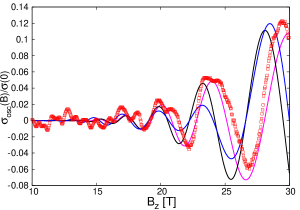
Figure 8: Comparison of the theoretical results and the measurements of Cui et al. [18]. The measured conductance oscillations $\sigma_{xx,exp}^{osc}$ (squares) and the fitting of the function $f_{osc}(B_{z})$ (see Eq. (7hijksuv)) using $n_{e}=1.1*10^{13}/{\rm cm}^{2}$, $2\Delta_{cb}=3\,$meV (blue) $n_{e}=1.31*10^{13}/{\rm cm}^{2}$, $2\Delta_{cb}=3\,$meV (black), and $n_{e}=1.31*10^{13}/{\rm cm}^{2}$, $2\Delta_{cb}=5\,$meV (purple).

Using $f_{0}(B_{z})$ we then extracted the oscillatory part $\sigma_{xx,osc}(B_{z})=\sigma_{xx,exp}(B_{z})-f_{0}(B_{z})$ of the conductance and fitted it with the function

$$f_{osc}(B_{z})=-A\frac{4(\mu_{q}B_{z})^{2}}{(1+(\mu_{q}B_{z})^{2})^{2}}\exp\left(\frac{-\pi}{\mu_{q}B_{z}}\right)\left[D_{1}\cos\left(\frac{2\pi E_{F}}{\hbar\omega_{\rm cb}}\right)+D_{2}\cos\left(\frac{E_{F}-2\Delta_{cb}}{\hbar\omega_{\rm cb}}\right)\right]$$ (7hijksuv)

where $D_{1,2}$ are fitting parameters. As one can see in Figure 8, the fit can qualitatively reproduce the meauserements, but the complex oscillations between $15-22$T are not captured. We also note that a somewhat better fit can be obtained if we assume that the charge density is larger than what is deduced from the classical Hall measurements (see the black line in Figure 8) and if we choose the spin-splitting larger than the value obtained from DFT calculations (purple line). In all cases we find, however, that the fit parameters $D_{1}$ and $D_{2}$ differ quite significantly in their magnitude, which is difficult to interpret in the present theoretical framework. This might indicate that additional scattering channels, such as inter-valley scattering, would have to be taken into account for a quantitative theory.

Finally, we would briefly comment on the relevance of the other valleys in the band structure for the SdH oscillations. Regarding p-doped samples, the $\Gamma$ point might, in principle, be important for MoS₂. However, according to DFT calculations [3] and ARPES measurements [49] the effective mass at the $\Gamma$ point is significantly larger than at $\pm K$ and therefore we do not expect that states at $\Gamma$ would lead to additional SdH oscillations. Nevertheless, they can be important for the level broadening of the sates at $\pm K$ because scattering from $\pm K$ to $\Gamma$ does not require a spin-flip [3]. In the case of other monolayer TMDCs the $\Gamma$ valley is most likely too far away in energy from the top of the VB at $\pm K$ to influence the transport for realistic dopings [3]. The situation can be more complicated for n-doped samples, especially for WS₂ and WSe₂. For these two materials the states in the six $Q$ valleys are likely to be nearly degenerate with the states in the $\pm K$ valleys. Therefore the $Q$ valleys might be relatively easily populated for finite n-doping and, in contrast to the $\Gamma$ point, the effective mass is comparable to that in the $\pm K$ [3] valleys. Therefore they may contribute to the SdH oscillations. They would also affect the level broadening of the $\pm K$ valley states because scattering from $K$ ($-K$) to three of the six $Q$ valleys is not forbidden by spin selection rules [3]. Furthermore, we note that in the absence of a magnetic field the six $Q$ valleys are pairwise connected by time reversal symmetry. Therefore, taking into account only the lowest-in-energy spin-split band in the $Q$ valleys, the LLs belonging to the $Q$ valleys will be three-fold degenerate: the magnetic field, similarly to the case of the $K$ and $-K$ points, would lift the six-fold valley-degeneracy. The effective valley g-factors, however, might be rather different from the ones in the $\pm K$ valleys. For n-doped monolayer MoX₂ materials the situation is probably less complicated because the $Q$ valleys are higher in energy and are not as easily populated as for the WX₂ monolayers. For MoS₂ monolayers, therefore, one can neglect the $Q$ valleys in first approximation.

4 Summary

In summary, we have studied the LL spectrum of monolayer TMDCs in a $\mathbf{k}\cdot\mathbf{p}$ theory framework. We have shown that in a wide magnetic field range the effects of the trigonal warping in the band structure are not very important for the LL spectrum. Therefore the LL spectrum can be approximated by a harmonic oscillator spectrum and a linear-in-magntic field term which describes the VDB. This approximation and the assumption that only intra-valley intra-band scattering is relevant allowed us to extend previous theoretical work on SdH oscillations to the case of monolayer TMDCs. In the semiclassical limit, where analytical calculations are possible, it is found tha the VDB affects the amplitude of the SdH oscillations, whereas the spin-splitting of the bands leads to a phase difference in the oscillatory components. Since in actual experimental situations there might be only a few occupied LL below $E_{F}$, we have also performed numerical calculations for the conductance oscillations and compared them to the analytical results. As it can be expected, if there are only a few LLs populated the amplitude of the SdH oscillations obtained in the semiclassical limit does not agree very well with the results of numerical calculations. This should be taken into account in the analysis of the experimental measurements. We used our theoretical results to analyze the measured SdH oscillations of Reference [18]. It is found that the quantum scattering time relevant for the SdH oscillations is significantly shorter than the transport scattering time that can be extracted from the Hall mobility. Finally, we briefly discussed the effect of other valleys in the band structure on the SdH oscillations.

5 Acknowledgement

A.K. thanks Xu Cui for discussions and for sending some of their experimental data prior to publication. This work was supported by Deutsche Forschungsgemeinschaft (DFG) through SFB767 and the European Union through the Marie Curie ITN S3NANO. P. R. would like to acknowledge the support of the Hungarian Scientific Research Funds (OTKA) K108676.

References

References

- [1] Xu X, Yao W, Xiao D, and Heinz T F, 2014 Nature Physics 10, 343.
- [2] Liu G-B, Xiao D, Yao Y, Xu X, and Yao W, 2015 Chem. Soc. Rev., Advance Article
- [3] Kormányos A, Burkard G, Gmitra M, Fabian J, Zólyomi V, Drummond N D, and Fal’ko V I, 2015 2D Materials 2, 022001.
- [4] Mak K F, Lee C, Hone J, Shan J, and Heinz T F, 2010 Phys. Rev. Lett. 105, 136805.
- [5] Xiao D, Liu G B, Feng W, Xu X, and Yao W, 2012 Phys. Rev. Lett. 108, 196802.
- [6] Mak K F, He K, Shan J, and Heinz T F, 2012 Nature Nanotechnology 7, 494.
- [7] Zeng H, Dai J, Yao W, Xiao D, and Cui X, 2012 Nature Nanotechnology 7, 490.
- [8] Cao T, Wang G, Han W, Ye H, Zhu Ch, Shi J, Niu Q, Tan P, Wang E, Liu B, and Feng J, 2012 Nature Communications 3, 887.
- [9] Sallen G, Bouet L, Marie X, Wang G, Zhu C R, Han W P, Lu Y, Tan P H, Amand T, Liu B L, and Urbaszek B, 2012 Phys. Rev. B 86, 081301.
- [10] Korn T, Heydrich S, Hirmer M, Schmutzler J, and Schüller C, 2011 Appl. Phys. Lett. 99, 102109.
- [11] Jones A M, Yu H, Ghimire N, Wu S, Aivazian G, Ross J S, Zhao B, Yan J, Mandrus D, Xiao D, Yao W, and Xu X, 2013 Nature Nanotechnology 8, 634.
- [12] Sie E J, McIver J W, Lee Y-H, Frenzel A J, Fu L, Kong J, and Gedik N, 2014 Nature Materials 14, 290.
- [13] Wang G, Marie X, Gerber I, Amand T, Lagarde D, Bouet L, Vidal M, Balocchi A, and Urbaszek B, 2015 Phys. Rev. Lett. 114, 097403.
- [14] Radisavljević B, Radenović A, Brivio J, Giacometti V, Kis, A, 2011 Nature Nanotechnology 6, 147.
- [15] Wang J , Yang Y, Chen Y-A, Watanabe K, Taniguchi T, Churchill H O H, and Jarillo-Herrero P, 2015 Nano Letters 15, 1898.
- [16] Kappera R, Voiry D, Yalcin S E, Branch B, Gupta G, Mohite A D, and Chhowalla M, 2014 Nature Materials 13, 1128.
- [17] Chuang H-J, Tan X, Ghimire N J, Perera M M, Chamlagain B, Cheng M M-Ch, Yan J, Mandrus D, Tománek D, and Zhou Z, 2014 Nano Letters 14, 3594.
- [18] Cui X, Lee G-H, Kim Y D, Arefe G, Huang P Y, Lee Ch-H, Chenet D A, Zhang X, Wang L, Ye F, Pizzocchero F, Jessen B S, Watanabe K, Taniguchi T, Muller D A, Low T, Kim P, and Hone J, 2015 Nature Nanotechnology, 10 534. (see also Preprint arXiv:1412.5977).
- [19] Liu Y, Wu H, Cheng H C, Yang S, Zhu E, He Q, Ding M, Li D, Guo J, Weiss N O, Huang Y, and Duan X, 2015 Nano Letters 15 3030.
- [20] Xu Sh, Han Y, Long G, Wu Z, Chen X, Han T, Ye W, Lu H, Wu Y, Lin J, Shen J, Cai Y, He Y, Lortz R, and Ning Wang, 2015 Preprint arXiv:1503.08427.
- [21] Radisavljevic B and Kis A, 2013 Nature Materials 12 815.
- [22] Baugher B W H, Churchill H O H, Yang Y, and Jarillo-Herrero P, 2013 Nano Letters 13, 4212.
- [23] Neal A T, Liu H, Gu J, and Ye P D, 2013 ACS Nano 8, 7077.
- [24] Schmidt H, Yudhistira I, Chu L, Castro Neto A H, Özyilmaz B, Adam S, and Eda G, 2015 Preprint arXiv:1503.00428
- [25] Lu H-Zh, Yao W, Xiao D and Shen Sh-Q, 2013 Phys. Rev. Lett. 110, 016806.
- [26] Ochoa H, Finocchiaro F, Guinea F, and Fal’ko V I, 2014 Phys. Rev. B 90, 235429.
- [27] Chu R-L, Li X, Wu S, Niu Q, Yao W, Xu X, and Zhang Ch, 2014 Phys. Rev. B 90, 045427.
- [28] Ho Y-H, Chiu Ch-W, Su W-P, and Lin M-F, 2014 Appl. Phys. Lett. 105, 222411.
- [29] Rostami H and Asgari R, 2015 Phys. Rev. B 91 075433.
- [30] Li X, Zhang F, and Niu Q, 2013 Phys. Rev. Lett. 110, 066803.
- [31] Cai T, Yang S A, Li X, Zhang F, Shi J, Yao W, and Niu Q, 2013 Phys. Rev. B 88, 115140.
- [32] Rose F, Goerbig M O, and Piéchon F, 2013 Phys. Rev. B 88, 125438.
- [33] Rostami H, Moghaddam A G, and Asgari R, 2013 Phys. Rev. B 88, 085440.
- [34] Kormányos A, Zólyomi V, Drummond N D, and Burkard G, 2014 Phys. Rev. X 4, 011034.
- [35] Qiu D Y, da Jornada F H, and Louie S G, 2013 Phys. Rev. Lett. 111, 216805.
- [36] Ramasubramaniam A, 2012 Phys. Rev. B 86, 115409.
- [37] MacNeill D, Heikes C, Mak K F, Anderson Z, Kormányos A, Zólyomi V, Park J, and Ralph D C, 2015 Physical Review Letters 114, 037401.
- [38] Wang G, Bouet L, Glazov M M, Amand T, Ivchenko E I, Palleau E, Marie X, and Urbaszek B, 2015 2D Materials 2 034002.
- [39] Adams E N, and Holstein T D, 1959 J. Phys. Chem. Solids 10, 254.
- [40] Zhou X, Liu Y, Zhou M, Tang D, and Zhou G, 2014 J. Phys.: Condens Matter 26, 485008.
- [41] Yankowitz M, McKenzie D, and LeRoy B J, 2015 Phys. Rev. Lett. 115, 136803.
- [42] Ando T, 1974 J. Phys. Soc. Jpn. 37, 1233.
- [43] Vasko F T and Raichev O E, Quantum Kinetic Theory and Applications, Springer (2005).
- [44] Bruus H and Flensberg K, Many-Body Quantum Theory in Condensed Matter Physics, Oxford University Press (2006).
- [45] Raikh M R, and Shahbazyan T V, 1994 Phys. Rev. B 49, 5531.
- [46] Averkiev N S, Golub L E, Tarasenko S A, and Willander M, 2001 J. Phys.: Condens. Matter 13, 2517.
- [47] Raichev O E, 2008 Phys. Rev B 78, 125304.
- [48] Goerbig M O, Montambaux G, and Piéchon F, 2014 EPL 105 57005.
- [49] Jin W, Yeh P-CH, Zaki N, Zhang D, Sadowski J T, Al-Mahboob A, van der Zande A M, Chenet D A, Dadap J I, Herman I P, Sutter P, Hone J, and Osgood, R M Jr., 2013 Phys. Rev. Lett. 111, 106801.