A correction to the enhanced bottom drag parameterisation of tidal turbines

Abstract

Hydrodynamic modelling is an important tool for the development of tidal stream energy projects. Many hydrodynamic models incorporate the effect of tidal turbines through an enhanced bottom drag. In this paper we show that although for coarse grid resolutions (kilometre scale) the resulting force exerted on the flow agrees well with the theoretical value, the force starts decreasing with decreasing grid sizes when these become smaller than the length scale of the wake recovery. This is because the assumption that the upstream velocity can be approximated by the local model velocity, is no longer valid. Using linear momentum actuator disc theory however, we derive a relationship between these two velocities and formulate a correction to the enhanced bottom drag formulation that consistently applies a force that remains closed to the theoretical value, for all grid sizes down to the turbine scale. In addition, a better understanding of the relation between the model, upstream, and actual turbine velocity, as predicted by actuator disc theory, leads to an improved estimate of the usefully extractable energy. We show how the corrections can be applied (demonstrated here for the models MIKE 21 and Fluidity) by a simple modification of the drag coefficient.

1 Introduction

One of the key advantages of tidal energy as a renewable energy source, is the predictable nature of the resource. Methods for the detailed prediction of tidal dynamics using hydrodynamic numerical models have been developed over many years and have been applied for many different purposes. Less well understood is how the placement of tidal energy converters in the flow will modify the existing tidal currents at both local and regional scales [1]. The challenge here is that the detailed flow around a turbine is a three-dimensional phenomenon comprising far smaller length scales than those of the underlying tidal resource. A typical approach therefore is to model the turbine scale flow in a three-dimensional CFD simulation based on a actuator disc, blade element, or actuator-line model (see e.g. Sun et al. [22], Harrison et al. [10], Batten et al. [2], Malki et al. [15], Churchfield et al. [3]). The effects of the turbine in a large scale hydrodynamic model are then parameterised, based on properties extracted from the CFD model.

The main property of the turbine that needs to be parameterised is the amount of thrust force exerted by the turbine on the flow (and vice-versa) as a function of the flow speed. This also determines the amount of energy taken out of the flow. Thrust curves typically take the form of a quadratic function of current speed with a non-dimensional thrust coefficient, and can be derived as described above in a high-resolution CFD model, or in lab experiments. Turbine specific properties such as cut-in and rated speeds however, mean that the curve does not necessarily follow a quadratic and therefore the coefficient is not constant but itself varies as a function of flow speed.

It is important to note, that the turbine properties derived in e.g. a CFD model, or from lab experiments, typically consider the placing of a single turbine in uniform background flow. Speed dependent properties are then expressed in terms of the background velocity, which, because the velocity is slowed down in the presence of a turbine, is available as the undisturbed upstream velocity. In a finite width channel, blockage effects may also affect the resulting thrust curve but can be corrected for (see e.g. Garrett and Cummins [9], Whelan et al. [26]) to derive the thrust curve for an idealised free-standing turbine. In addition, the results may be dependent on the turbulent properties of the flow.

An approach followed in many models is to implement the thrust in the form of an equivalent drag force term. For depth-averaged models this effectively comes down to an increased bottom drag [13, 23, 19, 8, 16] Three-dimensional models may implement the drag as a force over the entire water column [5], or if the vertical resolution allows it the drag can be applied over a vertical cross section (e.g. Roc et al. [20]), i.e. an idealised actuator disc.

Since the thrust force is given as a function of the upstream velocity, it is important to consider what velocity to use for the equivalent drag force in the model. One option is to probe the numerical velocity solution somewhat upstream of the turbine location. This however brings with it various difficulties such as the question of how far upstream is appropriate, or the fact that the flow upstream might not actually return to the uniform background flow condition that was considered in the CFD model, due to bathymetric changes or the presence of other turbines. Additionally, the use of a non-local velocity is not desirable for numerical and computational purposes: it makes it hard to treat the term implicitly (in the time-integration sense), potentially leading to time step restrictions for stability, and memory access outside of a fixed numerical stencil, or across sub-domains in domain-decomposed parallel model, is computationally inefficient.

When enough mesh resolution is available, both in the horizontal and vertical dimensions, to resolve the flow through the turbine the relationship between the upstream velocity and the turbine velocity can be predicted using Linear Momentum Actuator Disc Theory (LMADT). Using this relationship the quadratic drag law can be reformulated into a function of the local velocity, thus overcoming the difficulties and ambiguities mentioned above. This is the approach followed in Roc et al. [20]. The typical width of a tidal turbine, order 20m, can however be orders of magnitude smaller than the spatial scales of the tidal flow so that resolving an individual turbine may become prohibitively expensive even in large-scale unstructured mesh models that allow for the efficient focusing of mesh resolution. Also this approach requires the alignment of the mesh with the position and direction of the turbine, thus limiting the flexibility to quickly evaluate different turbine positionings and angles.

If the mesh resolution available is such that computational cells are much larger than the turbine scale, the drag force is necessarily applied over a larger area. In a typical implementation a constant drag is applied over a single cell (the cell that contains the turbine). If the cell size is in fact large enough it may be expected (this will be further investigated in this paper), that the local velocity is not actually affected greatly by the presence of the drag term since the drag force is “smeared” out over a large area and the local cell velocity represents an average of the velocity in a large area around the turbine. In that case the difference between the undisturbed background flow and the local cell velocity may be neglected and the turbine can be implemented using a simple quadratic drag law, function of the local velocity.

As will be shown in this paper however, when the mesh resolution is refined such that mesh distances are closer to the turbine scale, this approximation is no longer tenable as the difference between upstream and local velocity becomes too large. As long as individual turbines are not resolved however, the approach in Roc et al. [20] is also not valid as the local velocity is still larger than the theoretical turbine velocity predicted by linear momentum actuator disc theory. In particular, for depth-averaged models the local velocity will remain higher than the actual turbine velocity even when the horizontal scales are sufficiently resolved. This is due to the fact that the drag acts on the entire water column and thus the depth-averaged model velocity will represent an average of the actual turbine velocity and a higher by-pass velocity above and below the turbine. Even in three-dimensional models the drag force is often applied over the entire water column [5], or limited to one or only a few layers [27, 11], and does not necessarily give an accurate representation of the actual turbine cross-section and thus the model velocity where the drag is applied is not necessarily equal to the real turbine velocity.

Here we demonstrate how the actuator disc computation may be modified to include the fact that the drag force numerically is applied over a different cross section than the actual turbine. Thus again an analytical relationship can be derived between the undisturbed upstream flow and the local cell velocity, and similarly the drag force can be reformulated as a drag law dependent on the local cell velocity. Like the approach in Roc et al. [20], this leads to a correction to the drag law, which in this case depends on the local cell width, but that nonetheless can easily be implemented in existing models, as will be demonstrated here for the Fluidity and MIKE 21 models.

An alternative method for the parameterisation of turbines in large-scale hydrodynamic models that also makes extensive use of actuator disc theory, is the line momentum sink method [7, 21]. Actuator disc theory is used to express the effect of turbines, and more specifically an entire fence of turbines, as a relative head loss across the whole near-field flow pattern starting from the assumed uniform upstream flow at one end , down to the end of individual turbine wakes at the point where uniform flow is again achieved (within the far-field wake of the fence). This head loss is then applied as a jump condition across an edge, or multiple aligned edges within the computational grid using a Discontinuous Galerkin discretisation of the depth-averaged shallow water equations. The advantage of this method that it incorporates a detailed LMADT treatment of the near-field effects, including blockage effects for multiple turbines in a fence. It does require however that these effects are treated at the sub-grid level, and is therefore only appropriate for hydrodynamic models with grid sizes larger than the length scale of the near-field/turbine wake (typically 10–20 turbine diameters) [7].

For any numerical modelling study it is important to look at the effect of changing the grid resolution on the results of interest. In the modelling guidelines for tidal resource assessments in [14], a range of grid resolutions is recommended depending on the stage of the resource assessment, ranging from kilometre scale for regional studies, down to a range of 500 m to 50 m for specific site feasibility studies. Since the wake of a turbine is a three-dimensional phenomenon, it is not expected that an accurate description of the near-field flow can be obtained with a depth-averaged model. Nevertheless, such models should be capable of studying far-field effects. This relies on the correct forces and their effect on the large-scale flow being modelled correctly. As this paper shows however, the results of the standard enhanced bottom drag parameterisation of the turbine thrust force will deteriorate as the mesh resolution falls below that of the near-field/wake length scale ($\approx 200-300$ m for a typical turbine). The correction proposed in this paper ensures that consistent results can be obtained with grid resolutions smaller than the length scale of the turbine wake, all the way down to the turbine scale.

2 Enhanced bottom drag formulation

In this section we will describe the enhanced bottom drag parameterisation of turbines used in many models [19, 6, 16, 27] and demonstrate some issues with mesh dependency. We will do this within the framework of MIKE 21 [25], a depth-averaged hydrodynamics model widely used in the marine renewable industry, and an equivalent drag-based implementation in Fluidity, an open source, finite element modelling package [18, 12]. By comparing results between the two models we verify that the implementation in the closed source model MIKE 21 is indeed based on the same theory that underlies our implementation in Fluidity, and that the same issues are observed.

The aim of the turbine parameterisation is to represent the drag force of the turbine on the flow, which is typically given as:

$$\vec{F}(\vec{u})=\tfrac{1}{2}\rho C_{t}(|\vec{u}|)A_{t}|\vec{u}|\vec{u},$$ (1)

here $\vec{u}$ is the flow velocity, $\rho$ the density of sea water, $C_{t}$ the dimensionless drag or thrust coefficient, and $A_{t}$ the effective cross-sectional area of the turbine in the flow. The drag coefficient $C_{t}$ may itself be a function of speed due to turbine properties such as rating, pitch control and the use of a cut-in speed. As discussed in the introduction the drag law, often derived from a small-scale three-dimensional CFD model, is typically expressed as a function of the undisturbed background flow velocity, which in the case of an idealised domain corresponds to the uniform velocity upstream of the turbine.

The depth-integrated shallow water equations (in conservation form) are given by

$$\frac{\partial H\vec{u}}{\partial t}+\nabla\cdot\left(H\vec{u}\otimes\vec{u}\right)+gH\nabla\eta+c_{b}|\vec{u}|\vec{u} =0,$$ (2)

$$\frac{\partial\eta}{\partial t}+\nabla\cdot\left(H\vec{u}\right) =0,$$ (3)

where $H$ is the total water depth between bottom and free surface, elevated at a level $z=\eta$, $\vec{u}$ is the depth-averaged velocity, $g$ the gravitational acceleration and $c_{b}$ is the bottom friction coefficient.

A local momentum balance in a fixed local horizontal area $A$ is derived by integrating (2) over this area, multiplied by $\rho$:

$$\frac{d}{dt}\int_{A}\rho H\vec{u}+\int_{\partial A}\rho H\left(\vec{n}\cdot\vec{u}\right)\vec{u}+\int_{A}\rho gH\nabla\eta+\int_{A}c_{b}\rho|\vec{u}|\vec{u}=0.$$ (4)

The second term represents momentum flux through the boundary $\partial A$. The third term can be rewritten as an integral of hydrostatic pressure around the three-dimensional water column below $A$. The last term represents a momentum sink term due to bottom friction.

To implement the turbine thrust force through an enhanced bottom friction, $c_{b}\to c_{b}+c_{t}$, we need the additional momentum sink to be equal to the force, $\vec{F}(\vec{u})$ in (1). To address the question of which velocity $\vec{u}$ is used to compute $\vec{F}(\vec{u})$, in a first attempt we simply employ the local, depth-averaged velocity and average the force over the area $A$. Thus, we require that

$$\int_{A}c_{t}\rho|\vec{u}|\vec{u}=\frac{\int_{A}\vec{F}(\vec{u})}{A}.$$ (5)

Combined with (1) , it readily follows that the enhanced bottom drag coefficient $c_{t}$ in this case should be set to:

$$c_{t}(\vec{u})=\frac{C_{t}(\vec{u})A_{t}}{2A}.$$ (6)

Since we consider the parameterisation of turbines in hydrodynamic models where mesh distances are larger than the size of an individual turbine, the force is applied over the smallest area possible, typically the area of a single mesh cell. Thus the area $A$ in (6) corresponds to the cell area over which the enhanced drag coefficient is applied. In models where the cell area is much larger than the turbine cross section $A_{t}$, the additional drag is small and therefore the presence of the turbine will not have a large effect on the numerical solution for $\vec{u}$ in that cell. As an example, for typical values of $C_{t}=0.6$, a mesh distance $\Delta x=200~{}m$ and turbine diameter $D=18~{}m$, if the drag is applied over a single square computational cell of $\Delta x\times\Delta x$, we get

$$c_{t}(\vec{u})=\frac{C_{t}\pi\left(\frac{D}{2}\right)^{2}}{2\Delta x^{2}}\approx 0.00122,$$ (7)

which is only half of a typical value of $c_{b}=0.0025$ for the background bottom friction coefficient.

Since the effect of the additional drag is relatively small it is to be expected that the assumption that the local velocity within the cell is close to the undisturbed background flow is valid for relatively coarse resolution models, and can therefore be used in the averaged force in the right-hand side of (5). As the resolution is increased however and the mesh distances become closer to the turbine scale, the drag is applied over a smaller area and the reduction in local flow speed may become much larger. Because of the quadratic dependency of the drag force on the flow speed, this may have a significant impact on the force that is applied in the model.

3 Local velocity drop in idealised channel

We investigate the mesh-dependent reduction in local flow speed in more detail in the following idealised set up: a turbine is placed in a rectangular channel of length 10 km and width 1 km. The depth at rest is set to 25m and a bottom friction of $c_{b}=0.0025$, equivalent to a Chézy coefficient of $62.6$ m^1/2s^-1, is applied. At the upstream boundary a uniform velocity of 3.0 ms^-1 is enforced. At the downstream end a Flather boundary condition is applied. The steady state solution without a turbine can be described as a balance between the free surface gradient and the bottom friction. The necessary free surface slope leads to a water level that is approximately $0.9$ m higher at the upstream boundary than at the downstream boundary. The decrease in water depth $H$ along the channel, in combination with the continuity equation, leads to an acceleration along the channel, with the speed increasing from $3.0$ ms^-1 to $\approx 3.12$ ms^-1 downstream. In a separate computation of the hydrodynamics without a turbine, it was verified in both Fluidity and MIKE 21, that the background flow velocity at the turbine location, halfway the channel, is approximately 3.055 ms^-1.

For the simulations with a turbine, the following turbine parameters were chosen: the thrust coefficient $C_{t}=0.6$ with a turbine diameter of $D=16$ m giving a turbine cross-sectional area of $A_{t}=201$ m². The simulations were performed using both MIKE 21 and Fluidity on a series of identical triangular meshes with uniform resolutions starting at a mesh size of $\Delta x=320$ m, doubling the resolution each time with the mesh size decreasing down to $\Delta x=20$ m. One extra, fine resolution mesh with a mesh size equal to the turbine diameter was then run, $\Delta x=D=16$ m. For the parameterisation of the turbine in Fluidity the enhanced bottom drag approach described in the previous section was chosen. Although Fluidity here uses a finite element scheme with discontinuous piecewise linear velocity and piecewise quadratic pressure solution (the mixed P1${}_{\text{DG}}$$-$P2 velocity–pressure element pair, see Cotter et al. [4]) a piecewise constant drag field was used to simplify the computations and to remain close to the numerics of MIKE which uses a finite volume scheme with higher order flux reconstructions. Although the exact details of the implementation in MIKE were not available, the results between Fluidity and MIKE were found to be close enough to extend the analysis based on the parameterisation used in Fluidity to that in MIKE 21.

Figure 1: The speed at the turbine location, inside the enhanced bottom drag cell, decreases with increasing resolution both in the Fluidity and MIKE results.

Figure 1 displays the obtained velocity in the cell in which the drag has been enhanced to parameterise the effect of a turbine. MIKE 21 employs a cell centred scheme, so for this model we report the value in the centre of the cell. In Fluidity’s numerical scheme, P1${}_{\text{DG}}$$-$P2, the velocity is represented by a linear function in each cell which is discontinuous between the cells. Here, and in the rest of the paper, the presented results for the local cell velocity are obtained by taking the cell average. From figure 1 it can be seen that the obtained velocity is indeed highly mesh-dependent, and drops with increased mesh resolution. Since the square of this velocity is used to implement the drag term, a 10% drop in the local velocity leads to an approximate 20% drop in the drag force.

In a model of a fully resolved turbine the local velocity is expected to drop. After all, the velocity through the turbine is known to be smaller due to momentum exchange with the turbine, whereas the bypass flow around the turbine is expected to accelerate. The deceleration of the flow through the turbine can be estimated using linear momentum actuator disc theory (LMADT, see [9] for an application of this theory to tidal turbines). The theory assumes inviscid flow and a uniform upstream velocity $u_{0}$. Furthermore, it defines a velocity $u_{1}$ through the turbine, and velocities $u_{3}$ and $u_{4}$ in respectively the wake and bypass flow (see figure 2). It also defines pressures: $p_{0}$ for the upstream pressure, $p_{1}$ and $p_{2}$ directly on either side of the turbine, and a uniform pressure $p_{4}$ downstream where the velocities $u_{3}$ and $u_{4}$ are defined. At the same downstream location, the cross-sectional area of the wake flow is defined as $A_{3}$. In addition, it defines the known cross sections $A_{c}$ for the total channel cross section and $A_{t}$ for the turbine cross section.

Through selective application of the continuity equation, momentum conservation and Bernoulli’s principle, seven equations can be derived for the unknowns $u_{1},u_{3},u_{4},p_{1},p_{2},p_{0}$ and $A_{3}$, given $u_{0}$ and $p_{4}$ as upstream and downstream boundary conditions respectively (see A). These equations can be simplified greatly by assuming $A_{t}\ll A_{c}$, which means no blockage effects are taken into account. For this case, $u_{4}=u_{0},p_{4}=p_{0}$ and the velocity through the turbine can be computed as (cf. equation (63) in the appendix):

$$u_{1}=\tfrac{1}{2}\left(1+\sqrt{1-C_{t}}\right)u_{0}.$$ (8)

For our idealised channel case considered above, we may compute $u_{1}=2.49$ ms^-1. As we will see however in the next section, the difference between upstream and turbine velocity is smaller in the numerical results because the drag force is spread out over an area with a larger width. As already discussed, this means that at very coarse mesh resolutions the velocity in the drag cell is hardly different from the upstream velocity. As the mesh resolution is refined however, and the force can thus be applied over a smaller width, this velocity will drop. This decrease in local velocity will continue with increasing mesh resolution, and only when the resolution is sufficient that the drag force can be applied numerically over exactly the same cross section as that of the turbine, e.g. in a three-dimensional model, should we expect this velocity to have reached the value of $u_{1}$ computed from standard actuator disc theory.

4 Predicting the reduced velocity in the enhanced drag cell

Figure 2: Approximation of the enhanced drag formulation by actuator disc theory. An upstream velocity $u_{0}$ is assumed to reduce to a “turbine” velocity $u_{1}$ inside the square in which the enhanced drag is applied. The effect of the enhanced drag is assumed to be equivalent to an actuator disc of width $\Delta y$, the width of the cell in the direction transverse to the flow. The relationship between $u_{1}$ and $u_{0}$ can be estimated using actuator disc theory which involves eliminating wake and bypass velocities $u_{3}$ and $u_{4}$ from a set of algebraic equations derived from selectively applying mass and momentum conservation and Bernoulli principles (see A).

To simplify matters, we first consider the case where the turbine is represented by a square area of enhanced drag instead of a triangle. Additionally, we assume that this square area is aligned with the flow. To this end we create a series of meshes with the same resolutions $\Delta x=320$ m to $\Delta x=16$ m as in the previous section, but with an embedded square centred around the turbine location, of dimensions $\Delta x\times\Delta x$. The square is divided into two triangles, and outside the square an unstructured triangular mesh of approximately uniform resolution is created, as indicated in figure 2.

When we neglect variations in the streamwise-direction (here denoted as the $x$-direction), the model results should correspond to those of an infinitely thin actuator disc as is considered in actuator disc theory. The actuator disc modelled by this shallow water model has a cross-sectional area of $\Delta yH$. Here, and in the rest of the paper, $\Delta y$ is the width of the drag area, in the cross-stream direction. In this section in particular $\Delta y=\Delta x$. Since we consider mesh resolutions where $\Delta y>D$, and additionally $H>D$, this “numerical” cross section will be much larger than the actual cross section $A_{t}$. Therefore, to predict the results of the shallow water model using actuator disc theory, we should be careful to use the cross section $\Delta yH$ applicable to this model. If we neglect any variations within the horizontal square, we may then hope to predict the velocity within the square as the disc velocity $u_{1}$ from this modified actuator disc theory calculation.

Following the assumption made above (5), the magnitude of the force applied in the enhanced bottom drag approximation is given by:

$$F=\tfrac{1}{2}\rho A_{t}C_{t}u_{1}^{2}.$$ (9)

Note that here we need to use the actual turbine cross section $A_{t}$ as that is the user input in this formulation to calculate the enhanced drag $c_{t}$ in (6). Further we assume that the velocity that is used to compute the force in this approximation, which is simply the local velocity in the drag cell, will be accurately predicted as the velocity $u_{1}$ in the modified actuator disc theory that follows below.

Following the steps in the derivation of (8), (63) in the appendix, but now applied to an actuator disc of cross section $\hat{A}_{t}=\Delta yH$, we first define a modified thrust coefficient (cf. (57) in the appendix):

$$\hat{C}_{t}:=\frac{F}{\tfrac{1}{2}\rho\hat{A}_{t}u_{0}^{2}}=\frac{A_{t}}{\hat{A}_{t}}\frac{u_{1}^{2}}{u_{0}^{2}}C_{t}.$$ (10)

Following the same derivation of (8), we then obtain a relationship between the local model velocity $u_{1}$ and the upstream velocity $u_{0}$ if in (8) we replace $C_{t}$ with $\hat{C}_{t}$. This gives an expression for the ratio $u_{1}/u_{0}$ than can be substituted in (10), to give:

$$\hat{C}_{t}=\frac{A_{t}}{\hat{A}_{t}}\left(\tfrac{1}{2}\left(1+\sqrt{1-\hat{C}_{t}}\right)\right)^{2}C_{t}.$$ (11)

After some algebraic manipulation, this can be reworked to

$$\hat{C}_{t}=\frac{\frac{A_{t}}{\hat{A}_{t}}C_{t}}{\left(1+\tfrac{1}{4}\frac{A_{t}}{\hat{A}_{t}}C_{t}\right)^{2}}.$$ (12)

Finally, the relationship between the local velocity $u_{1}$ within the cell that the enhanced drag is applied in, and the upstream velocity $u_{0}$ is given by

$$u_{1}=\frac{1}{1+\tfrac{1}{4}\frac{A_{t}}{\hat{A}_{t}}C_{t}}u_{0}.$$ (13)

Figure 3 shows that the speed predicted by (13) closely follows that computed with Fluidity. Note that the results here differ from the Fluidity results in figure 1. This is because in figure 1, the drag is applied over an arbitrary triangle in an unstructured, triangular mesh generated by the mesh generator with a characteristic edge length set to the value of $\Delta x$ on the $x$-axis. The meshes used for the results here, figure 1, are also unstructured, triangular and use the same characteristic edge lengths, but incorporate a square, consisting of two triangles, with dimensions $\Delta x\times\Delta x$ over which the drag is applied. Comparing the two figures, it can be observed that the drag being applied over a square area, aligned with the flow direction, leads to a different relationship between the upstream velocity and the velocity within the drag area, than when the drag is applied over a triangle. For this reason, in the following we will derive two different corrections to the enhanced bottom drag formulation for these two cases.

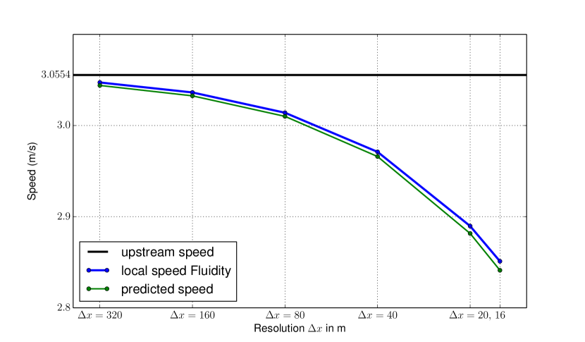
Figure 3: The speed inside a square drag cell decreasing with increasing resolution. Results are model outputs from Fluidity. The plotted speed is the average value over the square area. The decreasing cell speed can be accurately predicted using (13) derived from actuator disc theory.

5 Turbine correction for square cells

We have shown that actuator disc theory, using the width of a square enhanced drag cell and water depth, can accurately predict the relationship between upstream and local cell velocities. This can be used to reformulate the drag force applied in the cell to be a function not of the local cell velocity, but effectively of the upstream velocity. Instead of applying the force in (9), which is based on neglecting the difference between upstream and local velocity, we want to apply the force

$$F=\tfrac{1}{2}\rho A_{t}C_{t}u_{0}^{2},$$ (14)

where $u_{0}$ is the upstream velocity which is not readily (and locally) available. This expression is the same as in standard actuator disc theory, except now we need to take into account that this force is not applied over the cross-section $A_{t}$ but over a cross-section $\hat{A}_{t}=\Delta yH$. Thus we obtain a modified thrust coefficient:

$$\hat{C}_{t}:=\frac{F}{\tfrac{1}{2}\rho\hat{A}_{t}u_{0}^{2}}=\frac{A_{t}}{\hat{A}_{t}}C_{t}.$$ (15)

Note that this modified thrust coefficient differs from the one in the previous section, used to predict the results in the unmodified enhanced drag formulation, as we now assume that the correct force is applied.

Assuming $u_{1}$ is an adequate estimate for the local velocity in the cell with enhanced drag $c_{t}$ and cell area $A$, the force applied by the enhanced drag is given by (cf. the left-hand side of (5)):

$$F=\rho Ac_{t}u_{1}^{2}.$$ (16)

After updating (8) to use the modified thrust coefficient $\hat{C}_{t}$, we can substitute it here to make $F$ a function of the upstream velocity $u_{0}$:

$$F=\rho Ac_{t}\tfrac{1}{4}\left(1+\sqrt{1-\hat{C}_{t}}\right)^{2}u_{0}^{2}.$$ (17)

To obtain the appropriate value of $c_{t}$ we simply equate this expression with the desired force in (14). This leads to:

$$c_{t}=\frac{C_{t}A_{t}}{2A}\frac{4}{\left(1+\sqrt{1-\frac{A_{t}}{\hat{A}_{t}}C_{t}}\right)^{2}}.$$ (18)

In comparison with (6) from the standard enhanced bottom drag formulation, we have obtained an additional factor that corrects for the fact that we are using the local cell velocity instead of the upstream velocity. For coarse resolution runs, we have $A_{t}/\hat{A}_{t}\to 0$, and thus we fall back, as expected, to the unmodified enhanced drag formulation, since the cell velocity is close to the upstream velocity. As we have seen for finer resolutions, still coarser than the turbine scale, the difference between cell and upstream velocities becomes significant.

The correction derived above can also be applied to three-dimensional simulations with a resolved turbine, where the drag force is applied in three-dimensions over a vertical cross-sectional area (actuator disc) with $\hat{A}_{t}=A_{t}$ and therefore $\hat{C}_{t}=C_{t}$. The correction factor then simplifies to exactly that given in Roc et al. [20]. For the unresolved case however, both in two and three dimensions, the correction derived here not only corrects for the difference between upstream and turbine velocity, but also for the difference between the actual turbine cross-section and the cross-section over which the drag is applied numerically.

Returning to our idealised channel case, in figure 4 it is shown how the force in the standard enhanced bottom drag formulation applied to a square decreases with increasing mesh resolution. It is to be noted that the relative drop in drag force is larger than the relative drop in speed, due to the quadratic dependency of the force on the speed. Adjusting the drag formulation according to (18), the applied force is not only more accurate at coarse resolution, but also remains much closer to that computed from the upstream velocity directly as the mesh resolution approaches the turbine scale.

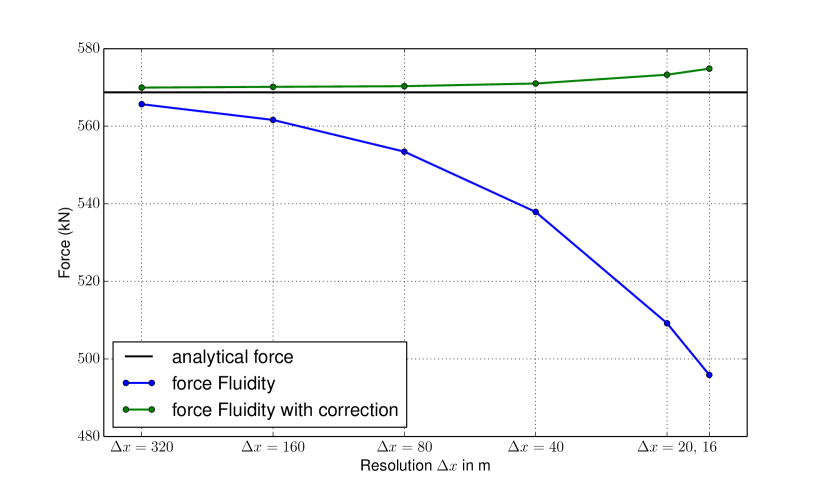
Figure 4: In the standard enhanced drag formulation for tidal turbines, equation (6), the applied force is a quadratic function of the local velocity in the drag cell (here, a square area of $\Delta x\times\Delta x$). As the mesh resolution increases, the local velocity drops, and therefore the force that is applied within the model decreases. Using the correction in (18) however, the same force can be maintained more or less independent of resolution.

6 Turbine correction for triangular cells

We now return to the case where the enhanced drag formulation is applied to a single triangular cell, not necessarily aligned in any way with the flow. Again we may approximate the applied drag by an actuator disc spanning the width of the triangle. In this case however, if we thus collapse the applied drag force to a single line, the amount of drag varies along the disc.

We assume here that the streamlines run parallel through the triangle and use a local coordinate system where $x$ is in the streamwise direction and $0\leq y\leq\Delta y$ in the transversal direction, where $\Delta y$ is the largest width of the triangle. We may subdivide the triangle into a number of streamtubes of infinitesimal width $\mathrm{d}y$, which can be considered as rectangles $\Delta x\times\mathrm{d}y$, whose length $\Delta x=\Delta x(y)$ is a function of $y$. When approximating this situation with actuator disc type theory, we make the following assumptions:

1. The drag in each streamtube, which in the numerical model is applied over a length $\Delta x(y)$, is collapsed in the $x$-direction and applied at a single point along the streamline, representing an infinitesimal actuator disc with cross section $H\mathrm{d}y$.

2. The results in each of the streamtubes are independent of one another. This means that we take no blockage effects into account and assume laminar flow.

For simplicity we first consider a triangle that is oriented in such a way that it is at its widest at $y=\Delta y$, in other words its top edge is aligned with the streamline at $y=\Delta y$ (see figure 5). Furthermore, we have $\Delta x(y=0)=0$ in the bottom vertex, and $\Delta x(y)$ varies linearly for $0\leq y\leq\Delta y$. Its area can be computed as $A=\tfrac{1}{2}\Delta x(\Delta y)\Delta y$. The function $\Delta x(y)$ is therefore given by:

$$\Delta x(y)=\frac{2A}{\Delta y^{2}}y.$$ (19)

The force applied in each streamtube is given by

$$\mathrm{d}F=\Delta x(y)\mathrm{d}y\rho c_{t}u_{1}(y)^{2},$$ (20)

where $u_{1}(y)$ is the velocity through the streamtube. Similar to (10), we apply actuator disc theory where we assume that this force is applied over a cross section $H\mathrm{d}y$ and obtain a modified thrust coefficient:

$$\hat{C}_{t}:=\frac{dF}{\tfrac{1}{2}\rho H\mathrm{d}yu_{0}^{2}}=\frac{2\Delta x(y)dy}{H\mathrm{d}y}\frac{u_{1}^{2}}{u_{0}^{2}}c_{t}$$ (21)

Following the same steps as in equations (10)–(13) we may derive the following relation between $u_{1}(y)$ and the upstream velocity $u_{0}$:

$$u_{1}(y)=\frac{1}{1+\tfrac{1}{2}\frac{\Delta x(y)\mathrm{d}y}{H\mathrm{d}y}c_{t}}u_{0}=\frac{1}{1+\frac{Ac_{t}}{H\Delta y^{2}}y}u_{0}.$$ (22)

The varying width $\Delta x(y)$ thus leads to a variation of the velocity $u_{1}(y)$ for $0\leq y\leq\Delta y$. In the computer models the accuracy of this variation is limited by the numerical approximations employed.

In MIKE, the underlying discretisation is based on a piecewise-constant velocity in each cell. To estimate the cell average obtained in the model we therefore evaluate (22) in the centroid at $y=\tfrac{2}{3}\Delta y$, which gives:

$$u^{\text{\tiny MIKE}}_{1}=\frac{1}{1+\tfrac{2}{3}\frac{Ac_{t}}{H\Delta y}}u_{0}.$$ (23)

For the case where the triangle does not have one of its edges aligned with a streamline, we may consider splitting the triangle into two triangles that share an edge that is aligned along the streamline (see figure 5). The length of this shared edge is the maximum width $\Delta x_{\text{max}}$ of the triangular drag cell in the streamwise direction. The area of either of the two triangles that the cell is split into, can be computed as $A_{1,2}=\tfrac{1}{2}\Delta x_{\text{max}}\Delta y_{1,2}$, where $\Delta y_{1,2}$ is the height of either triangle. Therefore for each of the triangles we have $A_{1,2}/\Delta y_{1,2}=\tfrac{1}{2}\Delta x_{\text{max}}$. Thus if we apply the same enhanced friction coefficient $c_{t}$ in both triangles, it follows that the estimate (23) for the cell average of $u^{\text{\tiny MIKE}}_{1}$ is the same in both triangles:

$$u^{\text{\tiny MIKE}}_{1}=\frac{1}{1+\tfrac{1}{3}\frac{\Delta x_{\text{max}}}{H}}u_{0}.$$ (24)

Moreover, if we define the overall cross-stream width of the original combined triangle as $\Delta y=\Delta y_{1}+\Delta y_{2}$, we again have $A/\Delta y=\tfrac{1}{2}\Delta x_{\text{max}}$. Thus, in the actual model where the original, non-aligned triangular drag cell is not split, we can use the same equation (23) for the estimated average velocity of the entire cell as we did for the aligned case.

Figure 5: Left figure: a triangle with its top edge aligned with the streamlines. A coordinate reference frame is chosen, with $0\leq y\leq\Delta y$ the coordinate in the cross-stream direction. The width $\Delta x$ of the triangle in the streamwise direction, varies as a function of $y$, starting at $\Delta x(y)=0$ at $y=0$, and reaching it maximum width $\Delta x(y)=\Delta x_{\text{max}}$ at $y=\Delta y$. Right figure: a non-aligned triangle can be divided in two triangles that share an edge that is aligned with the streamlines. In this case, the maximum width $\Delta x_{\text{max}}$ is the length of the shared edge.

Using this estimated average, the force applied in the model is then:

$$F=A\rho c_{t}(u^{\text{\tiny MIKE}}_{1})^{2}=A\rho c_{t}\left(\frac{1}{1+\tfrac{2}{3}\frac{Ac_{t}}{H\Delta y}}\right)^{2}u_{0}^{2}.$$ (25)

By equating this to the desired force (1), we may derive a quadratic expression for $c_{t}$

$$-2A^{2}A_{t}C_{t}c_{t}^{2}+A\left(9H^{2}\Delta y^{2}-6A_{t}C_{t}H\Delta y\right)c_{t}-\tfrac{9}{2}A_{t}C_{t}H^{2}\Delta y^{2}=0$$ (26)

In Fluidity, the P1${}_{\text{DG}}$-discretisation prescribes a linear variation for velocity. Thus we approximate (22) by evaluating it at $y=0$ and $y=\Delta y$ and assuming a linear variation in between:

$$u^{\text{\tiny Fluidity}}_{1}(y)=\left(1-\frac{1}{1+\frac{H\Delta y}{Ac_{t}}}\frac{y}{\Delta y}\right)u_{0}$$ (27)

The force applied in the model can be found by integrating:

$$F =\int_{y=0}^{\Delta y}\Delta x(y)\rho c_{t}(u^{\text{\tiny Fluidity}}_{1}(y))^{2}\mathrm{d}y$$ (28)

$$=A\rho c_{t}\left(1-\tfrac{4}{3}\left(\frac{1}{1+\frac{H\Delta y}{Ac_{t}}}\right)+\tfrac{1}{2}\left(\frac{1}{1+\frac{H\Delta y}{Ac_{t}}}\right)^{2}\right)u_{0}^{2}.$$ (29)

Equating with the desired force in (1) this time results in a cubic expression for $c_{t}$:

$$A^{3}c_{t}^{3}+A^{2}\left(4H\Delta y-3A_{t}C_{t}\right)c_{t}^{2}\\ +6A\left(H^{2}\Delta y^{2}-A_{t}C_{t}H\Delta y\right)c_{t}-3A_{t}C_{t}H^{2}\Delta y^{2}=0.$$ (30)

In case the triangular drag cell does not have an edge that is aligned with the streamlines, we may again consider splitting it into two triangles with a shared edge that is aligned with the flow. Here however, (27) does not predict the same linear function for $u^{\text{\tiny Fluidity}}_{1}$ in both triangles, since although $A/\Delta y=\tfrac{1}{2}\Delta x_{\text{max}}$ is the same, the value for $\Delta y$ in the denominator of $y/\Delta y$ is different for both triangles, and due to the different orientation of the top triangle, the sign of the gradient of $u^{\text{\tiny Fluidity}}_{1}$ with respect to $y$ will be opposite. The combined piecewise solution is therefore not supported by the underlying discretisation. However, we did find that when using the value of $c_{t}$ found by solving (30), the discrete model gave results that varied only slightly for different orientations of the triangular cell.

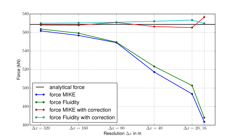
Figure 6: Results for the enhanced drag formulation with the drag applied in a single triangular cell as implemented in both Fluidity and MIKE 21. As in figure 4, which show the results for the square case, the force applied decreases significantly with increasing mesh resolution. Applying the correction for $c_{t}$ however, given by solving (26) (MIKE 21) or (30) (Fluidity), the force can be kept more or less constant and much closer to the desired value.

The results in figure 6 indicate that again the force applied in the unmodified enhanced drag implementation, in Fluidity and MIKE reduces significantly with increasing mesh resolution. A modification to the enhanced bottom drag $c_{t}$ was derived in this section, solving for $c_{t}$ in (26) and (30) for MIKE and Fluidity respectively, that is shown here to lead to a force that remains close to the desired value. The correction in MIKE was implemented by first finding the value for $c_{t}$ from (26) and then working back from (6) to compute what value of $C_{t}$ should be entered in the GUI to achieve this value in MIKE.

7 Power production

The correction to the enhanced drag formulation, derived in this paper, is to ensure that the correct amount of momentum is extracted from a shallow water model. This means that the force $F$ applied by the enhanced drag in the drag cell (or region) is an accurate approximation of the real thrust exerted by the turbine on the flow. The amount of energy taken out of the flow within the cell is given by:

$$P_{\text{cell}}=Fu_{1,\text{model}},$$ (31)

where $u_{1,\text{model}}$ is the velocity in the enhanced drag cell. As we have seen however, in the case where turbines are not fully resolved this velocity will be larger than the real velocity $u_{1,\text{turbine}}$ that goes through the turbine (as predicted by actuator disc theory). Therefore, the real power production $P_{\text{turbine}}=Fu_{1,\text{turbine}}$ will be smaller than the amount of power $P_{\text{cell}}$ taken out of the model in the drag cell.

This discrepancy can be explained from the fact that part of the mixing losses are not modelled explicitly within the model, but occurs at the sub-grid scale. Following the analysis of Vogel et al. [24], the total amount of power taken out of the flow can be split as follows:

$$P_{\text{total}}=P_{\text{turbine}}+P_{\text{mixing}},$$ (32)

where $P_{\text{mixing}}$ takes account of the mixing losses due to a.o. shear between the wake and bypass flows. The total power can be computed as [24]:

$$P_{\text{total}}=Fu_{0}.$$ (33)

Therefore, as long as the model applies an accurate representation of the thrust force $F$, using the correction presented in this paper, and an accurate value for the upstream velocity $u_{0}$, the total power extracted from the flow in the model will be accurate as well. The fact that the power $P_{\text{cell}}$ extracted within the drag cell, according to (31), is larger than $P_{\text{turbine}}$ means that the mixing loss that occurs in the model (outside the drag cell) must be smaller than the real $P_{\text{mixing}}$ predicted by actuator disc theory. Therefore part of the mixing loss occurs within the drag cell itself. Thus $P_{\text{cell}}$ accounts for both the power $P_{\text{turbine}}$ taken out by the turbine itself and additional losses that happen at the sub-grid level.

Vogel et al. [24] considers the case where the drag of an entire farm is smeared out over an enhanced drag region, with the assumption that all mixing losses actually occur within this region. In that case it may be assumed that the total power extraction in the model is a good approximation of the total power extraction predicted by actuator disc theory, so that the available usefully extracted power can be computed as a fraction of that using the same theory.

For the case, considered in this paper, where individual turbines are modelled but are not necessarily fully resolved, part of the mixing losses are modelled explicitly. As argued above however, using the power extracted from the flow by the turbine parameterisation still leads to an overprediction of the usefully extractable energy. It is to be noted that in a shallow water model, even if an individual turbine is resolved in the horizontal mesh, with a minimum mesh distance smaller or equal than the turbine diameter $D$, the effective cross-section $\hat{A}_{t}=\Delta yH$ will still be larger than the actual turbine cross-section $A_{t}$. This is because the actual cross-section does not span the entire depth of the water. Thus, the velocity at the turbine in the model should be interpreted as a depth-averaged velocity that averages between the velocity through the turbine, and the bypass velocity above and below the turbine. This velocity is therefore expected to be higher than the real turbine velocity itself, and therefore the power extraction by the depth-averaged turbine-parameterisation will always be an overprediction of the actual power available to the turbine. The difference between these power values roughly corresponds to vertical mixing losses that are not explicitly modelled in the depth-averaged model. In the next section we will explain how the relationship between the upstream velocity and the local velocity in the model, derived in this paper, can also be used to predict the usefully extractable energy, excluding mixing losses, more accurately.

8 Implementation details

In this section we summarise, how the analysis derived in this paper can be practically applied in existing models, in order to ensure that the correct force is applied on the flow and an accurate estimate of the available turbine power can be made.

8.1 Turbine drag applied over a rectangular area

For models where the turbine parameterisation consists of an enhanced bottom drag applied over a fixed, rectangular area $A$ (e.g. [23]), we may use the analysis presented in section 5. Where existing models typically make no distinction between upstream and local turbine velocity, they calculate the enhanced drag coefficient as $c_{t}=C_{t}A_{t}/2A$. Such implementations can be improved using the correction given by (18). The extra factor at the end of (18) can easily be included by the user in either $C_{t}$ or $A_{t}$, without the need for code modification, if these are the input parameters to the model.

An additional complexity arises if $C_{t}$ itself is not a constant. This occurs for example if a cut-in speed and/or rating are applied to the turbine. In this case, $C_{t}$ is typically given as a function (thrust curve) of the upstream velocity $u_{0}$. In the model however only the local velocity $u_{1}$ is available. Using the formula

$$u_{1}=\tfrac{1}{2}\left(1+\sqrt{1-\hat{C}_{t}}\right)u_{0},\quad\hat{C}_{t}=\frac{A_{t}}{\hat{A}_{t}}C_{t},$$ (34)

however, it is straight-forward to transform a lookup table that gives the thrust coefficient for different values of $u_{0}$, into a lookup table that is a function of $u_{1}$, by computing $u_{1}$ for the given values of $u_{0}$ as a pre-processing step.

For the computation of the power available to the turbine, we may use (64). Here, again we use (34) to derive the upstream velocity $u_{0}$ from the local cell velocity $u_{1}$. Combining these two equations, we derive:

$$P_{\text{turbine}}=\frac{2\left(1+\sqrt{1-C_{t}}\right)}{\left(1+\sqrt{1-\hat{C}_{t}}\right)^{3}}C_{t}\rho A_{t}u_{1}^{3}.$$ (35)

Again, in the case that $C_{t}$ is not a constant, a lookup table may be used to obtain the correct value of $P_{\text{turbine}}$ for each value of $u_{1}$.

8.2 Turbine parameterisation in an arbitrary triangular mesh

For models such as MIKE 21 and Fluidity that employ triangular meshes and which implement turbines through an increased drag applied within a single triangle, the theory presented in section 6 can be applied. In triangular mesh models where the drag force is based on a cell-averaged velocity, the value for the enhanced drag coefficient can be found by solving (26) for $c_{t}$. Models that use a linear interpolation of velocities stored in the vertices, such as Fluidity should use the value of $c_{t}$ found by solving (30). The same approach could also be followed to implement a turbine in a single drag cell in Telemac 2D, where its Finite Element modus is expected to behave in a similar manner as Fluidity, using a linear representation of the velocity within a cell.

In models, like MIKE, where the applied drag force and the associated coefficient $c_{t}$ are not explicitly prescribed, the same effect can be achieved by modifying the value of $C_{t}$. This is done by assuming the implementation is equivalent to the standard enhanced bottom drag formulation according to equation (6). Indeed the results in figure 1 where the standard drag implementation of Fluidity is compared with results in MIKE show that this is true to at least a good approximation. By providing MIKE with a modified value of $C_{t}$

$$C_{t,\text{modified}}=\frac{2Ac_{t}}{A_{t}},$$ (36)

we can therefore create the effect of applying a value of $c_{t}$ obtained from (26) without modifying the code. Note, that in equation (26) we use the original value of $C_{t}$ for the real turbine.

For non-constant $C_{t}$ that is given as a thrust curve, MIKE (and similar models) use the local cell velocity $u_{1}$ instead of the upstream velocity to look up the value of $C_{t}$. This can be corrected by converting the upstream values $u_{0}$ in a $u_{0}\to C_{t}$ look-up table into cell velocities $u_{1}$ using equation (23).

To compute the power that can be usefully extracted by the turbine we again use (64) this time combined with (23), giving:

$$P_{\text{turbine}}=\tfrac{1}{4}\left(1+\sqrt{1-C_{t}}\right)C_{t}A_{t}\left(1+\tfrac{2}{3}\frac{Ac_{t}}{H\Delta y}\right)^{3}(u^{\text{\tiny MIKE}}_{1})^{3}.$$ (37)

For finite element models, such as Fluidity, that consider a linear variation of the velocity within the cell we can use (27) which predicts the relationship between the upstream velocity and the velocity in the cell as a function of $y$. By first taking an average of the finite element solution $u^{\text{\tiny Fluidity}}_{1}$ within the drag cell in the streamwise direction ($x$-direction), we can then use this equation to estimate the upstream velocity $u_{0}$. This estimate may in practice still vary in the cross-streamwise direction ($y$-direction), so we take the cell average of its cube to obtain an estimate for $u_{0}^{3}$ in (64). Combining all this gives:

$$P_{\text{turbine}} =\tfrac{1}{4}\left(1+\sqrt{1-C_{t}}\right)\rho\frac{C_{t}A_{t}}{A}\int_{y=0}^{\Delta y}\Delta x(y)\left(\frac{\frac{\int_{x=0}^{\Delta x(y)}u^{\text{\tiny Fluidity}}_{1}dx}{\Delta x(y)}}{1-\frac{1+H\Delta y}{Ac_{t}}\frac{y}{\Delta y}}\right)^{3}dy.$$ (38)

8.3 Support structure

The drag exerted on the flow by the support structure, e.g. pylons or tripods, can typically also be parameterised as a force that depends quadratically on the upstream velocity $u_{0}$:

$$F_{\text{support}}=\tfrac{1}{2}\rho C_{s}A_{s}u_{0}^{2},$$ (39)

where $A_{s}$ and $C_{s}$ are the cross-sectional area and the drag coefficient of the support structure. To include this drag in the form of an enhanced bottom drag coefficient, we have to deal with the same issue of expressing this force in terms of a local velocity $u_{1}$. Although the theory derived so far can be straightforwardly applied to any force in this quadratic form, we cannot simply derive the enhanced bottom drag coefficient that represents the support drag, denoted by $c_{s}$, independently of $c_{t}$ and add them up. This is because the local velocity $u_{1}$ is the depth-averaged velocity that will be slowed down by the two sources of drag simultaneously.

For the drag parameterisation applied over a square area, the correct value for $u_{1}$ is obtained from (34) by using

$$\hat{C_{t}}=\frac{A_{t}C_{t}+A_{s}C_{s}}{H\Delta y}.$$ (40)

We can then derive a combined enhanced drag coefficient

$$c_{t}=\frac{A_{t}C_{t}+A_{s}C_{s}}{2A}\frac{4}{\left(1+\sqrt{1-\hat{C_{t}}}\right)^{2}},$$ (41)

that represents both turbine and support drag (cf. equation (18)). The effectively extracted power is still given by (35) using the combined value of $\hat{C_{t}}$ from (40), but only using the values for the turbine itself for $C_{t}$ and $A_{t}$.

For models where the drag is applied over a triangular cell, the relation between $u_{0}$ and $u_{1}$ is expressed in terms of the actual enhanced bottom drag coefficient $c_{t}$. Thus if we include both turbine and support drag in $c_{t}$, we can maintain equations (23) and (27) for models with cell-wise constant, and piecewise linear velocities respectively. The actual combined value of $c_{t}$ can then be found from the quadratic and cubic equations (26) and (30) respectively, by replacing $A_{t}C_{t}$ with $A_{t}C_{t}+A_{s}C_{s}$. Finally, the extracted power is still given by (37), using only the turbine values for $C_{t}$ and $A_{t}$, but using the combined value of $c_{t}$.

9 Conclusions

In order to accurately estimate the resource available to tidal turbines and to assess their impact on the hydrodynamics, it is important to accurately represent the drag force exerted by the turbines on the flow. In depth-averaged, and more generally under-resolved hydrodynamic models, one should keep in mind that the local model velocity at the turbine is different from both the upstream and the actual velocity passing through the turbine. The relationship between them is dependent on the mesh resolution, and in the case of depth-averaging, the ratio between the actual turbine cross section and the flow cross section spanning the entire depth. Therefore, although the use of the local velocity for the implementation of the drag force is computationally attractive, it is required to take these relationships into account to avoid spurious and mesh-dependent results. In addition, a better understanding of the relation between local and upstream velocity is necessary for an accurate estimate of the power available to the turbine.

Here we have presented the theory for a single, isolated turbine, and demonstrated that a correction based on linear momentum actuator disc theory taking into account the actual numerical cross section that the force is applied over in the model, can be used to obtain results that are consistent over a range of grid scales. It was shown that the standard enhanced bottom drag formulation results in a drag force that decreases with decreasing grid lengths, in particular when the grid size falls below the length scale of the turbine wake (roughly 10–20 turbine diameters). With the correction the applied force can be kept constant to a large degree, thus ensuring that the effect of the turbine on the large scale flow is correctly modelled.

The analysis for single, isolated turbines may be sufficient for sparsely populated turbine sites which see little interaction between turbines. It is generally recognised however, that in order to achieve the maximum available energy from certain sites, one needs to consider turbine configurations that benefit from local and global blockage effects [17], e.g. fence structures. The analysis in this paper could be extended to include blockage effects. Here again one should make a distinction between the influence of blockage on the relation between upstream and turbine velocities in reality, and the influence of blockage on the relation between upstream and local velocities in the model, in particular taking into account the difference in effective cross sections between reality and the model.

With more closely packed turbines the representation of turbine wake structures and wake recovery also becomes much more important. In addition, the turbulence characteristics may have a great impact on the performance of the turbines. As mentioned in the introduction, depth-averaged models will not be sufficient to accurately model these three-dimensional near-field effects. In further work we would like to explore however, how well these effects can still be approximated in depth-averaged models, possibly through parameterisation and tuning of horizontal turbulence models. Nonetheless, we recognise that in general it may no longer be possible to simply extrapolate from the results of a single isolated turbine, and it may be required to study the effects of combining multiple turbines in detailed three-dimensional CFD calculations and lab experiments.

10 Acknowledgements

The authors would like to kindly acknowledge the UK’s Engineering and Physical Sciences Research Council (EPSRC), projects EP/J010065/1 and EP/M011054/1, for funding which supported this work. Part of the computations in this work have been made possible using the Imperial College High Performance Computing Service.

Appendix A Linear Momentum Actuator Disc Theory

In this appendix we briefly review the main steps in the derivation of the actuator disc theory used in tidal turbine calculations. This is so we can refer to the relevant equations when the modifications, that take into account the numerical implementation details of the enhanced bottom drag formulation, are derived in the main text. These results can be found in e.g. Garrett and Cummins [9], or Whelan et al. [26].

We consider a channel of cross-sectional area $A_{c}$ in which a turbine is located with cross section $A_{t}$. We assume a uniform flow across the channel upstream of the turbine with velocity $u_{0}$, the flow through the turbine is $u_{1}$. Further downstream we define $u_{3}$ to be the velocity in the wake, and $u_{4}$ the bypass velocity. Furthermore we assume that at the point down-stream where $u_{3}$ and $u_{4}$ are defined we have a uniform water level $\eta_{4}$. The water level upstream is denoted by $\eta_{0}$, and the water levels just upstream and downstream of the turbine, associated with the pressure drop across the turbine are denoted by $\eta_{1}$ and $\eta_{2}$.

First we formulate the conservation of mass for the flow through the turbine and in the bypass flow

$$A_{t}u_{1} =A_{3}u_{3},$$ (42)

$$A_{c}u_{0} =A_{3}u_{3}+(A_{c}-A_{3})u_{4},$$ (43)

where $A_{3}$ is the cross-sectional area of the wake at the location where $u_{3}$ is defined. Here we neglect the influence of the water level on the cross sections, so that the cross-sectional area of the bypass flow is given by $A_{c}-A_{3}$. Inclusion of the dependency of cross section on the water level is only significant for high Froude numbers, with details given in [26].

The force $F$ exerted by the turbine on the flow (and vice-versa), can be related to a conservation of momentum principle in the entire channel, or to the pressure drop across the turbine:

$$F =A_{c}\rho u_{0}^{2}-A_{3}\rho u_{3}^{2}-(A_{c}-A_{3})\rho u_{4}^{2}+\rho gA_{c}(\eta_{0}-\eta_{4}),$$ (44)

$$F =\rho gA_{t}(\eta_{1}-\eta_{2}),$$ (45)

where $g$ is the gravitational acceleration. Finally, applying Bernoulli’s principle along streamlines: 1) from upstream, where $u_{0}$ is considered uniform, to just before the turbine, where water level $\eta_{1}$ is defined; 2) from just after the turbine, where water level $\eta_{2}$ is defined, to downstream where a uniform water level $\eta_{4}$ is defined; and 3) in the bypass flow from upstream to downstream. This yields three more equations:

$$\tfrac{1}{2}u_{0}^{2}+g\eta_{0} =\tfrac{1}{2}u_{1}^{2}+g\eta_{1},$$ (46)

$$\tfrac{1}{2}u_{1}^{2}+g\eta_{2} =\tfrac{1}{2}u_{3}^{2}+g\eta_{4},$$ (47)

$$\tfrac{1}{2}u_{0}^{2}+g\eta_{0} =\tfrac{1}{2}u_{4}^{2}+g\eta_{4}.$$ (48)

Assuming boundary conditions for $u_{0}$ and $\eta_{4}$, and an expression for $F$ as a function of $u_{0}$, we have seven equations for seven unknowns: $u_{1},u_{3},u_{4},\eta_{0},\eta_{1},\eta_{2},$ and $A_{3}$.

General solutions

The Bernoulli equations (46) to (48) can be rewritten as expressions for water level differences:

$$g\eta_{1}-g\eta_{2} =g\eta_{0}-g\eta_{4}+\tfrac{1}{2}\left(u_{0}^{2}-u_{3}^{2}\right),$$ (49)

$$g\eta_{0}-g\eta_{4} =\tfrac{1}{2}\left(u_{4}^{2}-u_{0}^{2}\right),$$ (50)

and thus

$$g\eta_{1}-g\eta_{2}=\tfrac{1}{2}\left(u_{4}^{2}-u_{3}^{2}\right).$$ (51)

We can therefore rewrite the two expressions (44) and (45) as:

$$F =A_{3}\rho\left(u_{4}^{2}-u_{3}^{2}\right)-\tfrac{1}{2}A_{c}\rho\left(u_{4}^{2}-u_{0}^{2}\right)$$ (52)

$$F =\tfrac{1}{2}A_{t}\rho\left(u_{4}^{2}-u_{3}^{2}\right)$$ (53)

Equations (43), (52) and (53) give three equations for the three unknowns $u_{3},u_{4}$ and $A_{3}$. Substitution of $A_{3}(u_{4}-u_{3})=A_{c}(u_{4}-u_{0})$ from (43), in (52) eliminates $A_{3}$:

$$\begin{split}F&=A_{3}\rho\left(u_{4}-u_{3}\right)(u_{4}+u_{3})-\tfrac{1}{2}A_{c}\rho\left(u_{4}^{2}-u_{0}^{2}\right)\\ &=A_{c}\rho\left(u_{4}-u_{0}\right)(u_{4}+u_{3})-\tfrac{1}{2}A_{c}\rho\left(u_{4}^{2}-u_{0}^{2}\right)\\ &=A_{c}\rho\left(u_{4}-u_{0}\right)\left(u_{3}+\tfrac{1}{2}u_{4}-\tfrac{1}{2}u_{0}\right).\end{split}$$ (54)

We can rearrange (53) and (54) in the following manner, respectively:

$$A_{c}^{2}\left(u_{4}-u_{0}\right)^{2}u_{3}^{2} =A_{c}^{2}\left(u_{4}-u_{0}\right)^{2}\left(u_{4}^{2}-\frac{2F}{A_{t}\rho}\right),$$ (55)

$$A_{c}^{2}\left(u_{4}-u0\right)^{2}u_{3}^{2} =\left(F-\tfrac{1}{2}A_{c}\rho\left(u_{4}-u_{0}\right)^{2}\right)^{2}.$$ (56)

We introduce the additional definitions,

$$C_{t}:=\frac{F}{\tfrac{1}{2}A_{t}\rho u_{0}^{2}},\quad\text{ and }\quad\epsilon:=\frac{A_{t}}{A_{c}}.$$ (57)

Note that we do not have to assume that $F$ is actually quadratic in $u_{0}$, so that $C_{t}$ is not necessarily a constant; it may still be dependent on $u_{0}$. With these we can derive the following quartic polynomial in $u_{4}$ from (55) and (56):

$$\frac{1}{4}\left(C_{t}\epsilon-\left(\frac{u_{4}}{u_{0}}-1\right)^{2}\right)^{2}-\left(\frac{u_{4}}{u_{0}}-1\right)^{2}\left(\frac{u_{4}^{2}}{u_{0}^{2}}-C_{t}\right)=0.$$ (58)

Finally, by (53):

$$u_{3}=\sqrt{u_{4}^{2}-C_{t}u_{0}^{2}},$$ (59)

and $A_{3}$ can be derived by again substituting (43) in (52) but this time to eliminate $A_{c}(u_{4}-u0)$, so that

$$F=A_{3}\rho\left(u_{4}-u_{3}\right)\left(u_{3}+\tfrac{1}{2}u_{4}-\tfrac{1}{2}u_{0}\right),$$ (60)

which in combination with (53), gives:

$$A_{3}=\frac{\tfrac{1}{2}u_{4}+\tfrac{1}{2}u_{3}}{u_{3}+\tfrac{1}{2}u_{4}-\tfrac{1}{2}u_{0}}A_{t}.$$ (61)

Zero blockage limit

From the above, it follows that in the limit $\epsilon\to 0$: $u_{4}\to u_{0}$ and thus $\eta_{4}\to\eta_{0}$. In this limit, (59) becomes

$$u_{3}\to\sqrt{1-C_{t}}~{}u_{0},$$ (62)

and combining (61) and (42):

$$u_{1}=\frac{\tfrac{1}{2}u_{4}+\tfrac{1}{2}u_{3}}{u_{3}+\tfrac{1}{2}u_{4}-\tfrac{1}{2}u_{0}}u_{3}\to\tfrac{1}{2}\left(1+\sqrt{1-C_{t}}\right)u_{0}.$$ (63)

The energy yield then becomes:

$$P=Fu_{1}\to\tfrac{1}{4}\left(1+\sqrt{1-C_{t}}\right)C_{t}A_{t}\rho u_{0}^{3}.$$ (64)

The maximum yield as a function of $C_{t}$ is obtained by:

$$\frac{d}{dC_{t}}\left[\left(1+\sqrt{1-C_{t}}\right)C_{t}\right]=\frac{1-\tfrac{3}{2}C_{t}+\sqrt{1-C_{t}}}{\sqrt{1-C_{t}}}=0$$ (65)

$$\implies\left(\tfrac{3}{2}C_{t}-1\right)^{2}=1-C_{t}\implies C_{t}=\frac{8}{9}.$$ (66)

Thus the maximum power (assuming no blockage) is

$$P_{\text{max}}=\frac{16}{27}\cdot\tfrac{1}{2}A_{t}\rho u_{0}^{3}\approx 0.59\cdot\tfrac{1}{2}A_{t}\rho u_{0}^{3}.\quad\text{({\bf Betz limit})}$$ (67)

References

- Adcock et al. [2015] Adcock, T. A., Draper, S., Nishino, T., 2015. Tidal power generation – a review of hydrodynamic modelling. Proceedings of the Institution of Mechanical Engineers, Part A: Journal of Power and Energy, 0957650915570349.
- Batten et al. [2013] Batten, W. M., Harrison, M., Bahaj, A., 2013. Accuracy of the actuator disc–RANS approach for predicting the performance and wake of tidal turbines. Philosophical Transactions of the Royal Society A: Mathematical, Physical and Engineering Sciences 371 (1985), 20120293.
- Churchfield et al. [2013] Churchfield, M. J., Li, Y., Moriarty, P. J., 2013. A large-eddy simulation study of wake propagation and power production in an array of tidal-current turbines. Philosophical Transactions of the Royal Society A: Mathematical, Physical and Engineering Sciences 371 (1985), 20120421.
- Cotter et al. [2009] Cotter, C. J., Ham, D. A., Pain, C. C., 2009. A mixed discontinuous/continuous finite element pair for shallow-water ocean modelling. Ocean Modelling 26 (1-2), 86–90.
- Defne et al. [2011] Defne, Z., Haas, K. A., Fritz, H. M., 2011. Numerical modeling of tidal currents and the effects of power extraction on estuarine hydrodynamics along the georgia coast, usa. Renewable Energy 36 (12), 3461–3471.
- Divett et al. [2013] Divett, T., Vennell, R., Stevens, C., 2013. Optimization of multiple turbine arrays in a channel with tidally reversing flow by numerical modelling with adaptive mesh. Philosophical Transactions of the Royal Society A: Mathematical, Physical and Engineering Sciences 371 (1985), 20120251.
- Draper et al. [2010] Draper, S., Houlsby, G., Oldfield, M., Borthwick, A., 2010. Modelling tidal energy extraction in a depth-averaged coastal domain. IET renewable power generation 4 (6), 545–554.
- Funke et al. [2014] Funke, S. W., Farrell, P. E., Piggott, M., 2014. Tidal turbine array optimisation using the adjoint approach. Renewable Energy 63, 658–673.
- Garrett and Cummins [2007] Garrett, C., Cummins, P., 2007. The efficiency of a turbine in a tidal channel. Journal of Fluid Mechanics 588, 243–251.
- Harrison et al. [2010] Harrison, M., Batten, W., Myers, L., Bahaj, A., 2010. Comparison between CFD simulations and experiments for predicting the far wake of horizontal axis tidal turbines. IET Renewable Power Generation 4 (6), 613–627.
- Hasegawa et al. [2011] Hasegawa, D., Sheng, J., Greenberg, D. A., Thompson, K. R., 2011. Far-field effects of tidal energy extraction in the Minas Passage on tidal circulation in the Bay of Fundy and Gulf of Maine using a nested-grid coastal circulation model. Ocean Dynamics 61 (11), 1845–1868.
-
Imperial College London, Applied Modelling and Computation Group
(2015) [AMCG]
Imperial College London, Applied Modelling and Computation Group (AMCG),
2015. Fluidity manual v4.1.12.
URL http://dx.doi.org/10.6084/m9.figshare.1387713 - Lalander and Leijon [2009] Lalander, E., Leijon, M., 2009. Numerical modeling of a river site for in–stream energy converters. In: Proc. 8th European Wave and Tidal Energy Conf., Sweden.
- Legrand [2009] Legrand, C., 2009. Assessment of tidal energy resource: Marine renewable energy guides. Tech. rep.
- Malki et al. [2013] Malki, R., Williams, A., Croft, T., Togneri, M., Masters, I., 2013. A coupled blade element momentum–computational fluid dynamics model for evaluating tidal stream turbine performance. Applied Mathematical Modelling 37 (5), 3006–3020.
- Martin-Short et al. [2015] Martin-Short, R., Hill, J., Kramer, S., Avdis, A., Allison, P., Piggott, M., 2015. Tidal resource extraction in the Pentland Firth, UK: Potential impacts on flow regime and sediment transport in the Inner Sound of Stroma. Renewable Energy 76, 596–607.
- Nishino and Willden [2012] Nishino, T., Willden, R. H., 2012. The efficiency of an array of tidal turbines partially blocking a wide channel. Journal of Fluid Mechanics 708, 596.
- Piggott et al. [2008] Piggott, M., Gorman, G., Pain, C., Allison, P., Candy, A., Martin, B., Wells, M., 2008. A new computational framework for multi-scale ocean modelling based on adapting unstructured meshes. International Journal for Numerical Methods in Fluids 56 (8), 1003–1015.
- Plew and Stevens [2013] Plew, D. R., Stevens, C. L., 2013. Numerical modelling of the effect of turbines on currents in a tidal channel – Tory Channel, New Zealand. Renewable Energy 57, 269–282.
- Roc et al. [2013] Roc, T., Conley, D. C., Greaves, D., 2013. Methodology for tidal turbine representation in ocean circulation model. Renewable Energy 51, 448–464.
- Serhadlıoğlu et al. [2013] Serhadlıoğlu, S., Houlsby, G., Adcock, T., Draper, S., Borthwick, A., 2013. Assessment of tidal stream energy resources in the UK using a discontinuous Galerkin finite element scheme. In: 17th Int. Conf. on Finite Elements in Flow Problems, San Diego, CA, 24–27 February 2013.
- Sun et al. [2008] Sun, X., Chick, J., Bryden, I., 2008. Laboratory-scale simulation of energy extraction from tidal currents. Renewable Energy 33 (6), 1267–1274.
- Vennell [2010] Vennell, R., 2010. Tuning turbines in a tidal channel. Journal of Fluid Mechanics 663, 253–267.
- Vogel et al. [2013] Vogel, C., Wilden, R., Houlsby, G., 2013. A correction for depth-averaged simulations of tidal turbine arrays. In: EWTEC 2013 Proceedings.
- Warren and Bach [1992] Warren, I., Bach, H., 1992. MIKE 21: a modelling system for estuaries, coastal waters and seas. Environmental Software 7 (4), 229–240.
- Whelan et al. [2009] Whelan, J., Graham, J., Peiro, J., 2009. A free-surface and blockage correction for tidal turbines. Journal of Fluid Mechanics 624, 281–291.
- Yang et al. [2013] Yang, Z., Wang, T., Copping, A. E., 2013. Modeling tidal stream energy extraction and its effects on transport processes in a tidal channel and bay system using a three-dimensional coastal ocean model. Renewable Energy 50, 605–613.