Siklos waves in Poincaré gauge theory

Abstract

A class of Siklos waves, representing exact vacuum solutions of general relativity with a cosmological constant, is extended to a new class of Siklos waves with torsion, defined in the framework of the Poincaré gauge theory. Three particular exact vacuum solutions of this type, the generalized Kaigorodov, the homogeneous and the exponential solution, are explicitly constructed.

1 Introduction

The first complete formulation of the idea of (internal) gauge invariance was given in Weyl’s classic paper [1]. A significant progress in this direction has been achieved somewhat later by Yang, Mills and Utiyama [2, 3]. It opened a new perspective for understanding gravity as a gauge theory, the perspective that was realized by Kibble and Sciama [4] in their proposal of a new theory of gravity, known as the Poincaré gauge theory (PGT). The PGT is a gauge theory of the Poincaré group, with an underlying Riemann-Cartan (RC) geometry of spacetime [5, 6]. In this approach, basic gravitational variables are the tetrad field $b^{i}$ and the Lorentz connection $\omega^{ij}$ (1-forms), and the related field strengths are the torsion $T^{i}=db^{i}+\omega^{i}{{}_{m}}\wedge b^{mj}$ and the curvature $R^{ij}=d\omega^{ij}+\omega^{i}{{}_{m}}\wedge\omega^{mj}$ (2-forms). At a more physical level, the source of gravity in PGT is matter possessing both the energy-momentum and spin currents. The importance of the Poincaré symmetry in particle physics leads one to consider PGT as a favorable framework for describing the gravitational phenomena.

Based on the experience stemming from Einstein’s general relativity, it is known that exact solutions play a crucial role in developing our understanding of the geometric and physical content of a gravitational theory; for a review, see Refs. [7, 8, 9, 10]. An important set of these solutions refers to exact gravitational waves, the structure of which has been studied also in PGT [11]. In the present work, we focus on a particular class of the gravitational waves, the class of Siklos waves that are vacuum solutions of general relativity with a cosmological constant (GR_Λ), propagating on the AdS background [12]. By generalizing the ideas developed in three dimensions [13], we construct here a class of the four-dimensional Siklos waves with torsion as vacuum solutions of PGT.

The paper is organized as follows. In section 2, we give a short account of the Siklos waves in the tetrad formulation of GR_Λ. In section 3, we show that Siklos waves are torsion-free vacuum solutions of PGT. In section 4, we introduce new vacuum solutions of PGT, the Siklos waves with torsion, by modifying the Siklos geometry in a manner that preserves the radiation nature of the original configuration. That is achieved by an ansatz for the RC connection that produces only the tensorial irreducible mode of the torsion with $J^{P}=2^{+}$. The PGT field equations are simplified and shown to depend only on three parameters, including the mass of the torsion mode. In sections 5, 6 and 7, we describe three different vacuum solutions belonging to the class of Siklos waves with torsion: the generalized Kaigorodov, the homogeneous and the exponential solution. section 7 is devoted to concluding remarks, and two appendices contain some technical details.

Our conventions are as follows. We use the Poincaré coordinates $x^{\mu}=(u,v,x,y)$ as the local coordinates; the Latin indices $(i,j,...)$ refer to the local Lorentz (co)frame and run over $(+,-,2,3)$, $b^{i}$ is the tetrad (1-form), $h_{i}$ is the dual basis (frame), such that $h_{i}\,\hbox{\vrule height=0.0pt,width=4.0pt,depth=0.3pt\vrule height=7.0pt,width=0.3pt,depth=0.3pt\vrule height=0.0pt,width=2.0pt,depth=0.0pt}\hskip 0.8pt\,b^{k}=\delta_{i}^{k}$; the volume 4-form is $\hat{\epsilon}=b^{+}\wedge b^{-}\wedge b^{2}\wedge b^{3}$, the Hodge dual of a form $\alpha$ is ${{}^{\star}}\alpha$, with ${{}^{\star}}1=\hat{\epsilon}$, totally antisymmetric tensor is defined by ${{}^{\star}}(b_{i}\wedge b_{j}\wedge b_{k}\wedge b_{m})=\varepsilon_{ijkm}$ and normalized to $\varepsilon_{+-23}=1$; in the rest of the paper, the exterior product of forms is implicit.

2 Siklos waves in GR_Λ

Siklos waves were introduced as a class of exact gravitational waves propagating on the AdS background [12]. In the Poincaré coordinates $x^{\mu}=(u,v,x,y)$, the Siklos metric is given by

$$ds^{2}=\frac{\ell^{2}}{y^{2}}\left[2du(Hdu+dv)-dx^{2}-dy^{2}\right]\,,$$ (2.1)

with $H=H(u,x,y)$. It admits the null Killing vector field $\partial_{v}$ that is not covariantly constant, the wave fronts are surfaces of constant $u$ and $v$, and the case $H=0$ corresponds to the AdS background. The metric (2.1) coincides with a special subclass of the Kundt class [9, 10], and is obviously conformal to pp-waves. The physical interpretation of the Siklos waves was investigated by Podolský [14, 15].

Now, we give a short account of the Siklos waves in the tetrad formulation of GR_Λ, which allows for a simpler generalization to PGT. First, we choose the tetrad field in the form

$$b^{+}:=\frac{\ell}{y}du\,,\qquad b^{-}:=\frac{\ell}{y}(Hdu+dv)\,,\qquad b^{2}:=\frac{\ell}{y}dx\,,\qquad b^{3}:=\frac{\ell}{y}dy\,,$$ (2.2)

so that the line element becomes $ds^{2}=2b^{+}b^{-}-(b^{2})^{2}-(b^{3})^{2}\equiv\eta_{ij}b^{i}b^{j}$, where $\eta$ is the half-null Minkowski metric,

$$\eta_{ij}=\left(\begin{array}[]{cccc}0&1&0&0\\ 1&0&0&0\\ 0&0&-1&0\\ 0&0&0&-1\end{array}\right)\,.$$

The dual frame $h_{i}$ is given by

$$h_{+}=\frac{y}{\ell}(\partial_{u}-H\partial_{v})\,,\qquad h_{-}=\frac{y}{\ell}\partial_{v}\,,\qquad h_{2}=\frac{y}{\ell}\partial_{x}\,,\qquad h_{3}=\frac{y}{\ell}\partial_{y}\,.$$ (2.3)

Next, we introduce the Riemannian connection $\omega^{ij}$ by imposing the condition of vanishing torsion, $\nabla b^{i}:=db^{i}+\omega^{i}{{}_{m}}b^{m}=0$, which yields

$$\omega^{+-},\omega^{+2}=0\,,\qquad\omega^{+3}=\frac{1}{\ell}b^{+}\,,\qquad\omega^{23}=\frac{1}{\ell}b^{2}\,,$$

$$\omega^{-2}=-\frac{y}{\ell}\partial_{x}Hb^{+}\,,\qquad\omega^{-3}=\frac{1}{\ell}b^{-}-\frac{y}{\ell}\partial_{y}Hb^{+}\,.$$ (2.4a)

The wave nature of the Siklos wave is clearly seen by rewriting $$\omega^{ij}$$ in the form

$$\omega^{ij}=\bar{\omega}^{ij}+k^{i}(h^{j}\,\hbox{\vrule height=0.0pt,width=4.0pt,depth=0.3pt\vrule height=7.0pt,width=0.3pt,depth=0.3pt\vrule height=0.0pt,width=2.0pt,depth=0.0pt}\hskip 0.8pt\,H)b^{+}\,,$$ (2.4b)

where $\bar{\omega}^{ij}=\omega^{ij}(H=0)$ refers to the AdS background, and the second term is the radiation piece, characterized by the null vector $k^{i}=(k^{+},k^{-},k^{2},k^{3})=(0,1,0,0)$.

Now, one can calculate the Riemannian curvature:

$$R^{+j}=\frac{1}{\ell^{2}}b^{+}b^{j}\,,\qquad R^{23}=\frac{1}{\ell^{2}}b^{2}b^{3}\,,$$

$$R^{-2}=\frac{1}{\ell^{2}}b^{-}b^{2}+\frac{1}{\ell^{2}}(y^{2}\partial_{xx}H-y\partial_{y}H)b^{+}b^{2}+\frac{1}{\ell^{2}}(y^{2}\partial_{xy}H)b^{+}b^{3}\,,$$

$$R^{-3}=\frac{1}{\ell^{2}}b^{-}b^{3}+\frac{1}{\ell^{2}}(y^{2}\partial_{yy}H-y\partial_{y}H)b^{+}b^{3}+\frac{1}{\ell^{2}}(y^{2}\partial_{xy}H)b^{+}b^{2}\,,$$ (2.5)

where we use $\partial_{xx}:=\partial^{2}/\partial x^{2}$ etc. The Ricci curvature ${Ric}^{i}=h_{m}\hbox{\vrule height=0.0pt,width=4.0pt,depth=0.3pt\vrule height=7.0pt,width=0.3pt,depth=0.3pt\vrule height=0.0pt,width=2.0pt,depth=0.0pt}\hskip 0.8ptR^{mi}$ and the scalar curvature $R=h_{i}\hbox{\vrule height=0.0pt,width=4.0pt,depth=0.3pt\vrule height=7.0pt,width=0.3pt,depth=0.3pt\vrule height=0.0pt,width=2.0pt,depth=0.0pt}\hskip 0.8pt{Ric}^{i}$ are found to be

$${Ric}^{m}=\frac{3}{\ell^{2}}b^{m}\,,\qquad m=+,2,3,$$

$${Ric}^{-}=\frac{3}{\ell^{2}}b^{-}+\frac{1}{\ell^{2}}(y^{2}\partial_{xx}H+y^{2}\partial_{yy}H-2y\partial_{y}H)b^{+}\,,$$

$$R=\frac{12}{\ell^{2}}\,.$$ (2.6)

Dynamical structure of GR_Λ is defined by the action $I_{\mit\Lambda}=-\int d^{4}x\sqrt{-g}\,(a_{0}R+2{\mit\Lambda})$. The corresponding vacuum field equations can be suitably written in the traceless form as

$${Ric}^{i}-\frac{1}{4}Rb^{i}=0\,.$$ (2.7)

As a consequence, the metric function $H$ must obey

$$y^{2}\left(\partial_{xx}H+\partial_{yy}H\right)-2y\partial_{y}H=0\,.$$ (2.8)

The profile ($u$-dependence) of the Siklos wave may be arbitrary.

We display here three special solutions of (2.8) discussed by Siklos [12]:

$$H_{1}=y^{3},\,{\rm Kaigorodov^{\prime}s~{}solution~{}(1963)};$$

$$H_{2}=\arctan(x/y)+xy/(x^{2}+y^{2})\,,\qquad\tilde{H}_{2}=(x^{2}+y^{2})H_{2};$$

$$H_{3}=C_{1}e^{x}(\cos y+y\sin y)+C_{2}e^{x}(\sin y-y\cos y)\,.$$

Note that Defrise’s metric (1969), with $H=1/y^{2}$, is not a vacuum solution of GR_Λ [15].

3 Siklos waves as torsion-free solutions of PGT

In this section, we show that the Siklos spacetime of the previous section is an exact Riemannian solution of PGT in vacuum.

Starting from the general PGT dynamics described in Appendix B, one can easily derive its reduced form in the Riemannian sector of PGT, characterized by $T^{i}=0$. First, we note that the only nonvanishing irreducible components of the Riemannian curvature are ${}^{(1)}R^{ij}$, ${}^{(4)}R^{ij}$ and ${}^{(6)}R^{ij}$, defined in Appendix A. And second, the condition $T^{i}=0$ implies that dynamical evolution of the Riemannian solutions in PGT is described by a reduced form of the general field equations (B.3):

$$(1ST) E_{i}=0\,,$$

$$(2ND) \nabla H_{ij}=0\,.$$ (3.1a)

Here, the Riemannian expressions for $$E_{i} H_{ij} T^{i}=0$$ and are obtained directly from the corresponding PGT formulas (see Appendix B) in the limit :

$$H_{ij}=-2a_{0}{{}^{\star}}(b^{i}b^{j})+2{{}^{\star}}(b_{1}{}^{(1)}R_{ij}+b_{4}{}^{(4)}R_{ij}+b_{6}{}^{(6)}R_{ij})\,,$$

$$E_{i}:=h_{i}\,\hbox{\vrule height=0.0pt,width=4.0pt,depth=0.3pt\vrule height=7.0pt,width=0.3pt,depth=0.3pt\vrule height=0.0pt,width=2.0pt,depth=0.0pt}\hskip 0.8pt\,L_{G}-\frac{1}{2}(h_{i}\,\hbox{\vrule height=0.0pt,width=4.0pt,depth=0.3pt\vrule height=7.0pt,width=0.3pt,depth=0.3pt\vrule height=0.0pt,width=2.0pt,depth=0.0pt}\hskip 0.8pt\,R^{mn})H_{mn}\,.$$ (3.1b)

As shown in Ref. [5], the field equations (3.1) are satisfied for any configuration in which the traceless symmetric Ricci tensor vanishes:

$${Ric}_{(ij)}-\frac{1}{4}\eta_{ij}R=0\,.$$ (3.2)

Comparing this result with the GR_Λ field equation (2.7), one concludes that any vacuum solution of GR_Λ is automatically a torsion-free solution of PGT. In particular, this is true for the Siklos metric.

It is useful to explore this general statement in details. Using the geometry of the Siklos spacetime found in the previous section, the content of Eqs. (3.1a) is found to be:

$$(1ST) \bigl{(}b_{4}+b_{6}-a_{0}\ell^{2}\bigr{)}y\Bigl{[}y(\partial_{xx}H+\partial_{yy}H)-2\partial_{y}H\Bigr{]}=0\,,$$

$$3a_{0}+\ell^{2}{\mit\Lambda}=0,$$

$$(2ND) (b_{1}+b_{4})y^{2}\partial_{x}\Bigl{[}y(\partial_{xx}H+\partial_{yy}H)-2\partial_{y}H\Bigr{]}=0\,,$$ (3.3)

$$(b_{1}+b_{4})y^{2}\partial_{y}\Bigl{[}y(\partial_{xx}H+\partial_{yy}H)-2\partial_{y}H\Bigr{]}=0\,.$$

For the generic values of the Lagrangian parameters $a_{0},b_{1},b_{4},b_{6}$, dynamical content of these equations is obviously the same as in GR_Λ, since the metric function $H$ must be such that

$${\hat{S}}H:=y\left(\partial_{xx}H+\partial_{yy}H\right)-2\partial_{y}H=0\,.$$ (3.4)

Thus, although PGT has a rather different dynamical structure as compared to GR_Λ, the class of Riemannian Siklos spacetimes is still an exact vacuum solution of PGT.

4 Siklos waves with torsion

We are now ready to generalize the previous results by constructing a new, non-Riemannian class of Siklos waves, the Siklos waves with torsion.

4.1 Geometry of the ansatz

We wish to introduce torsion in a manner that preserves the radiation nature of the Riemannian Siklos waves of GR_Λ, relying on the approach proposed in [13].

We start the construction by assuming that the tetrad field in PGT retains its Riemannian form (2.2). Then, by noting that the radiation piece of the Riemannin connection (2.4) has the form $(\omega^{ij})^{R}=k^{i}(h^{j\mu}\partial_{\mu}H)b^{+}$, we assume that the new RC connection is given by

$$\omega^{ij}=\bar{\omega}^{ij}+k^{i}h^{j\mu}(\partial_{\mu}H+K_{\mu})b^{+}\,,$$ (4.1a)

where the form of $$K_{\mu}$$ is defined by

$$K_{\mu}=(0,0,K_{x},K_{y})\,,$$

$$K_{x}=K_{x}(u,x,y)\,,\qquad K_{y}=K_{y}(u,x,y)\,.$$ (4.1b)

This ansatz modifies only two components of the Riemannian connection (2.4):

$$\omega^{-2}=-\frac{y}{\ell}(\partial_{x}H+K_{x})b^{+}\,,\qquad\omega^{-3}=\frac{1}{\ell}b^{-}-\frac{y}{\ell}(\partial_{y}H+K_{y})b^{+}\,.$$

The new terms in the connection are related to the torsion of spacetime:

$$T^{-}=\frac{y}{\ell}(K_{x}b^{+}b^{2}+K_{y}b^{+}b^{3})\,,\qquad T^{+},T^{2},T^{3}=0\,.$$ (4.2)

The only nonvanishing irreducible torsion piece is the tensor piece ${}^{(1)}T^{i}$, with ${}^{(1)}T^{-}=T^{-}$.

Denoting the Riemannian curvature found in section 2 by ${\mathaccent 869{R}}^{ij}$, the new, RC curvature is found to have the form:

$$R^{+j}=\frac{1}{\ell^{2}}b^{+}b^{j}\,,\qquad R^{23}=\frac{1}{\ell^{2}}b^{2}b^{3}\,,$$

$$R^{-2}={\mathaccent 869{R}}^{-2}+\frac{1}{\ell^{2}}(y^{2}\partial_{x}K_{x}-yK_{y})b^{+}b^{2}+\frac{1}{\ell^{2}}(y^{2}\partial_{y}K_{x})b^{+}b^{3}\,,$$

$$R^{-3}={\mathaccent 869{R}}^{-3}+\frac{1}{\ell^{2}}(y^{2}\partial_{y}K_{y})b^{+}b^{3}+\frac{1}{\ell^{2}}(y^{2}\partial_{x}K_{y}+yK_{x})b^{+}b^{2}\,.$$ (4.3a)

Note that the radiation piece of $$R^{ij} k^{i}=(0,1,0,0)$$ is proportional to the null vector . The corresponding Ricci and scalar curvatures are:

$${Ric}^{m}=\frac{3}{\ell^{2}}b^{a}\,,\quad m=+,2,3,$$

$${Ric}^{-}={\mathaccent 869{{Ric}}}{}^{-}+\frac{1}{\ell^{2}}(y^{2}\partial_{x}K_{x}+y^{2}\partial_{y}K_{y}-yK_{y})b^{+}\,,$$

$$R=\frac{12}{\ell^{2}}\,.$$ (4.3b)

The nonvanishing irreducible components of the curvature are ${}^{(n)}R^{ij}$ for $n=1,4,6$ (as in GR_Λ) and $n=2$. Quadratic invariants of the field strengths are regular:

$$R^{ij}{{}^{\star}}R_{ij}=\frac{12}{\ell^{4}}\,\hat{\epsilon}\,,\qquad T^{i}{{}^{\star}}T_{i}=0\,.$$

4.2 Field equations

Dynamical content of our ansatz is effectively described by the RC Lagrangian (B.1) with nonvanishing parameters $(a_{0},{\mit\Lambda};a_{1},b_{1},b_{2},b_{4},b_{6})$, and the associated PGT field equations (B.3). Explicit calculation of the 2nd field equation in (B.3), denoted shortly by ${\cal F}^{ij}$, is shown to have two nontrivial components, ${\cal F}^{-2}$ and ${\cal F}^{-3}$. After introducing the quantity ${\hat{S}}H$ as in Eq. (3.4), these components take the respective forms:

$$b_{1}\left(y\partial_{x}{\hat{S}}H+y^{2}\partial_{xx}K_{x}+y^{2}\partial_{yy}K_{x}-2y\partial_{x}K_{y}\right)$$

$$+b_{2}(y^{2}\partial_{yy}K_{x}-y^{2}\partial_{xy}K_{y}-y\partial_{x}K_{y})$$

$$+b_{4}\left(y\partial_{x}{\hat{S}}H+y^{2}\partial_{xx}K_{x}+y^{2}\partial_{xy}K_{y}-y\partial_{x}K_{y}\right)$$

$$+2(b_{6}-b_{1}+a_{1}\ell^{2}-a_{0}\ell^{2})K_{x}=0\,,$$ (4.4a)

and

$$b_{1}\left(y\partial_{y}{\hat{S}}H+y^{2}\partial_{xx}K_{y}+y^{2}\partial_{yy}K_{y}+2y\partial_{x}K_{x}\right)$$

$$+b_{2}(-y^{2}\partial_{xy}K_{x}+y^{2}\partial_{xx}K_{y}+y\partial_{x}K_{x})$$

$$+b_{4}\left(y\partial_{y}{\hat{S}}H+y^{2}\partial_{xy}K_{x}+y^{2}\partial_{yy}K_{y}+y\partial_{x}K_{x}\right)$$

$$+2(b_{6}-b_{1}+a_{1}\ell^{2}-a_{0}\ell^{2})K_{y}=0\,.$$ (4.4b)

The content of the 1st field equation is much simpler. To have the smooth limit for vanishing torsion, we require $$3a_{0}+\ell^{2}{\mit\Lambda}=0$$, whereupon the 1st equation reads

$$(b_{4}+b_{6}-a_{0}\ell^{2}){\hat{S}}H$$

$$+(b_{4}+b_{6}-a_{0}\ell^{2}+a_{1}\ell^{2})(y\partial_{x}K_{x}+y\partial_{y}K_{y}-K_{y})=0\,.$$ (4.4c)

The form of the differential equations (4.4) appears to be rather complicated [16]. However, there exists a suitable reformulation that makes their content much more transparent. To see that, we first rewrite Eq. (4.4c) in the form

$${\hat{S}}H=\sigma(y\partial_{x}K_{x}+y\partial_{y}K_{y}-K_{y})\,,\qquad\sigma:=-\left(1+\frac{a_{1}\ell^{2}}{b_{4}+b_{6}-a_{0}\ell^{2}}\right)\,.$$

Then, by substituting the expressions for $$y\partial_{x}{\hat{S}}H y\partial_{y}{\hat{S}}H (b_{1}+b_{4})(\sigma+1)$$ and into (4.4a) and (4.4b), and dividing the resulting equations by , one obtains

$$(y^{2}\partial_{xx}+\rho y^{2}\partial_{yy}+2\ell^{2}\mu^{2})K_{x}+\bigl{[}(1-\rho)y^{2}\partial_{xy}-(1+\rho)y\partial_{x}\bigr{]}K_{y}=0\,,$$ (4.5a)

$$(y^{2}\partial_{yy}+\rho y^{2}\partial_{xx}+2\ell^{2}\mu^{2})K_{y}+\bigl{[}(1-\rho)y^{2}\partial_{xy}+(1+\rho)y\partial_{x}\bigr{]}K_{x}=0\,.$$ (4.5b)

where

$$\rho:=\frac{b_{1}+b_{2}}{(b_{1}+b_{4})(\sigma+1)}\,,\qquad\mu^{2}:=\frac{a_{1}-a_{0}+(b_{6}-b_{1})/\ell^{2}}{(b_{1}+b_{4})(\sigma+1)}\,.$$

The final equations (4.4) contain only three independent parameters, $\sigma,\rho$ and $\mu^{2}$, which makes it much easier to find some specific solutions for the Siklos waves with torsion.

The parameter $\mu^{2}$ has a simple physical interpretation. As the linearized PGT analysis shows, possible torsion excitations around the Minkowski background are modes with spin-parity $J^{P}=0^{\pm},1^{\pm},2^{\pm}$ [18]. In particular, the spin-$2^{+}$ state is associated to the tensorial piece of the torsion, and its mass is

$$\bar{\mu}^{2}=\frac{a_{0}(a_{1}-a_{0})}{a_{1}(b_{1}+b_{4})}\,.$$

For $1/\ell^{2}\to 0$, the coefficient $\mu^{2}$ tends exactly to $\bar{\mu}^{2}$, whereas for finite (and positive) $\ell^{2}$, $\mu^{2}$ is associated to the spin-$2^{+}$ torsion excitation with respect to the AdS background.

In what follows, we will present three exact solutions of the PGT field equations (4.4), enlightening thereby basic dynamical aspects of the Siklos waves with torsion. All the integration “constants” appearing in these solutions are functions of $u$.

5 Kaigorodov-like solution

Motivated by the form of the Kaigorodov solution of GR_Λ (section 2), we consider now a class of PGT configurations for which the functions $H,K_{x}$ and $K_{y}$ are $x$-independent. Then, the field equations (4.5) take a much simpler form:

$$(\rho y^{2}\partial_{yy}+2\mu^{2}\ell^{2})K_{x}=0\,,$$ (5.1a)

$$(y^{2}\partial_{yy}+2\mu^{2}\ell^{2})K_{y}=0\,,$$ (5.1b)

$$y\partial_{yy}H-2\partial_{y}H=\sigma(y\partial_{y}-1)K_{y}\,.$$ (5.1c)

The Euler–Fuchs differential equation (5.1a) is solved by the ansatz $K_{x}=y^{\alpha}$, where $\alpha$ is restricted by the requirement $\alpha^{2}-\alpha+2\mu^{2}\ell^{2}/\rho=0$, which implies

$$\alpha_{\pm}=\frac{1}{2}\pm p\,,\qquad p:=\frac{1}{2}\sqrt{1-8\mu^{2}\ell^{2}/\rho}\,.$$ (5.2)

(a1) For $8\mu^{2}\ell^{2}/\rho<1$ (real $p$):

$$K_{x}=\sqrt{y}\left(A_{1}y^{p}+A_{2}y^{-p}\right)\,.$$ (5.3a)

(a2) For $$8\mu^{2}\ell^{2}/\rho>1 p q:=|p|$$ (imaginary , ):

$$K_{x}=\sqrt{y}\bigl{[}A_{3}\cos(q\ln y)+A_{4}\sin(q\ln y)\bigr{]}\,.$$ (5.3b)

(a3) For $$8\mu^{2}\ell^{2}/\rho=1 p=0$$ ():

$$K_{x}=\sqrt{y}\left(A_{5}+A_{6}\ln y\right)\,.$$ (5.3c)

Equation (5.1b) follows from (5.1a) in the limit $\rho\to 1$. Hence, using the notation

$${\bar{\alpha}}_{\pm}=\frac{1}{2}\pm{\bar{p}}\,,\qquad{\bar{p}}:=\frac{1}{2}\sqrt{1-8\mu^{2}\ell^{2}}\,,\qquad{\bar{q}}=|{\bar{p}}|\,,$$ (5.4)

the solutions for $K_{y}$ can be obtained from Eqs. (5.3) by the replacements $p\to{\bar{p}}$, $q\to{\bar{q}}$.
(b1) For $8\mu^{2}\ell^{2}<1$:

$$K_{y}=\sqrt{y}\left(B_{1}y^{\bar{p}}+B_{2}y^{-{\bar{p}}}\right)\,.$$ (5.5a)

(b2) For $$8\mu^{2}\ell^{2}>1$$:

$$K_{y}=\sqrt{y}\bigl{[}B_{3}\cos({\bar{q}}\ln y)+B_{4}\sin({\bar{q}}\ln y)\bigr{]}\,,$$ (5.5b)

(b3) For $$8\mu^{2}\ell^{2}=1$$:

$$K_{y}=\sqrt{y}\left(B_{5}+B_{6}\ln y\right)\,.$$ (5.5c)

Knowing the form of $K_{y}$, one can integrate Eq. (5.1c) to obtain the metric function $H$. Let us first find a particular solution $H_{(i)}$ of the inhomogeneous equation (5.1c).
(c1) For $8\mu^{2}\ell^{2}<1$:

$$H_{(i)}=\sigma y^{3/2}\left(\frac{({\bar{\alpha}}_{+}-1)}{({\bar{\alpha}}_{+}+1)({\bar{\alpha}}_{+}-2)}B_{1}y^{\bar{p}}+\frac{({\bar{\alpha}}_{-}-1)}{({\bar{\alpha}}_{-}+1)({\bar{\alpha}}_{-}-2)}B_{2}y^{-{\bar{p}}}\right)\,.$$ (5.6a)

(c2) For $$8\mu^{2}\ell^{2}>1$$:

$$H_{(i)}=\frac{2\sigma}{9+4{\bar{q}}^{2}}\,y^{3/2}\bigl{[}(B_{3}-2B_{4}{\bar{q}})\cos({\bar{q}}\ln y)+(B_{4}+2B_{3}{\bar{q}})\sin({\bar{q}}\ln y)\bigr{]}\,.$$ (5.6b)

(c3) For $$8\mu^{2}\ell^{2}=1$$:

$$H_{(i)}=\frac{2\sigma}{9}\,y^{3/2}\left(B_{5}-2B_{6}+B_{6}\ln y\right)\,.$$ (5.6c)

Adding to $H_{(i)}$ the solution of the homogeneous equation (5.1c), that is the Kaigorodov solution $H_{1}$ from section 2, one obtains the complete solution:

$$H=H_{1}+H_{(i)}\,,\qquad H_{1}=Dy^{3}\,.$$ (5.7)

Thus, the existence of torsion has a direct influence on the form of metric.

The above solutions for $K_{x},K_{y}$ and $H$ define a Kaigorodov wave with torsion as a vacuum solution of PGT.

Asymptotic AdS limit

It is interesting to note that the Kaigorodov solution in GR_Λ is asymptotically AdS, as follows from the asymptotic relation $H={\cal O}(y^{3})$ for $y\to 0$, and the form of the Riemannian curvature (2.5). In PGT, the presence of torsion makes the situation not so simple. Namely, the condition that the RC curvature $R^{ij}$ in (4.3) has the AdS asymptotics produces two types of requirements: the first one is obtained from the non-Riemannian piece of $R^{ij}$,

$$yK_{x}\to 0\,,\qquad yK_{y}\to 0\,,$$ (5.8a)

$$y^{2}\partial_{y}K_{x}\to 0\,,\qquad y^{2}\partial_{y}K_{y}\to 0\,,$$ (5.8b)

and the second from the Riemannian piece:

$$y\partial_{y}H_{(i)}\to 0\,,\qquad y^{2}\partial_{yy}H_{(i)}\to 0\,.$$ (5.8c)

Further analysis goes as follows.

(i) In the sector with $8\mu^{2}\ell^{2}/\rho\geq 1$ and $8\mu^{2}\ell^{2}\geq 1$, one can directly verify that the solutions for $K_{x},K_{y}$ and $H_{(i)}$ satisfy the requirements (5.8).

(ii) In the complementary sector with $8\mu^{2}\ell^{2}/\rho<1$ and $8\mu^{2}\ell^{2}<1$, one finds that the requirements (5.8) are valid for $p<1$ and ${\bar{p}}<1$, or equivalently, for

$$8\mu^{2}\ell^{2}/\rho>-1\quad{\rm and}\quad 8\mu^{2}\ell^{2}>-1\,.$$ (5.9)

Continuing with exploring the asymptotic properties of the torsion, we see that (5.8a) implies $T^{i}\to 0$ for $y\to 0$. Thus, the choice of parameters described in (5.9) ensures that the Kaigorodov-like solution has an AdS asymptotic behavior, with vanishing torsion. Clearly, in the physical sector with $\mu^{2}\geq 0$, the second condition in (5.9) is automatically satisfied.

Defrise-like solution as special case

It is interesting to observe that the form of $H_{(i)}$ in (5.6a) allows us to obtain a generalized Defrise solution, defined in section 2, as a special case of the Kaigorodov wave with torsion. Namely, by choosing $D=0$ one eliminates $H_{1}$ from $H$, whereupon the term $H_{(i)}$, specified by $B_{1}=0$ and ${\bar{p}}=7/2$, becomes identical to the Defrise metric function:

$$H=H_{(i)}\sim 1/y^{2}\,.$$ (5.10)

The restriction ${\bar{p}}=7/2$ refers to the tachyonic sector of the $2^{+}$ torsion mode, with $\mu^{2}\ell^{2}=-6$. The above result for $H$, combined with the corresponding expressions for $K_{x}$ and $K_{y}$, defines the Defrise solution with torsion as a vacuum solution of PGT. In contrast to that, the corresponding solution in GR_Λ exists only in the presence of matter. One should stress that the metric function $H$ originates purely from the torsional term $H_{(i)}$.

6 Homogeneous solution

Let us now look for a solution in which $K_{x},K_{y},H$ are homogeneous functions of $y$ and $x$:

$$K_{x}=f_{x}(t)\,,\qquad K_{y}=f_{y}(t)\,,\qquad H=h(t)\,,\qquad t:=y/x\,.$$

As a consequence, the field equations (4.5) become:

$$(t^{4}+\rho t^{2})f_{x}^{\prime\prime}+2t^{3}f_{x}^{\prime}+2\mu^{2}f_{x}-(1-\rho)t^{3}f_{y}^{\prime\prime}+2\rho t^{2}f_{y}^{\prime}=0\,,$$ (6.1a)

$$(t^{2}+\rho t^{4})f_{y}^{\prime\prime}+2\rho t^{3}f_{y}^{\prime}+2\mu^{2}f_{y}-(1-\rho)t^{3}f_{x}^{\prime\prime}-2t^{2}f_{x}^{\prime}=0\,,$$ (6.1b)

$${\hat{S}}H=\sigma(-t^{2}f^{\prime}_{x}+tf^{\prime}_{y}-f_{y})\,,$$ (6.1c)

where ${\hat{S}}H=y[2t(t^{2}-1)h^{\prime}+(t^{4}+t^{2})h^{\prime\prime}]$.

The set of equations (6.1) represents a system of ordinary, second-order, linear differential equations. The system is significantly simplified by assuming that the metric function $H$ retains the same form as in GR_Λ, so that ${\hat{S}}H=0$. Consequently, the right hand side of Eq. (6.1c) vanishes, $-t^{2}f^{\prime}_{x}+tf^{\prime}_{y}-f_{y}=0$, which implies

$$f_{x}=\frac{1}{t}f_{y}+B\,,$$ (6.2)

where $B=B(u)$. Substituting this expression into (6.1a) and (6.1b), one obtains

$$\rho t^{2}(t^{2}+1)f_{y}^{\prime\prime}+2\rho t(t^{2}-1)f_{y}^{\prime}+2(\rho+\mu^{2}\ell^{2})f_{y}+2\mu^{2}tB=0\,,$$ (6.3a)

$$\rho t^{2}(t^{2}+1)f_{y}^{\prime\prime}+2\rho t(t^{2}-1)f_{y}^{\prime}+2(\rho+\mu^{2}\ell^{2})f_{y}=0\,.$$ (6.3b)

Taking the difference of these two equations yields

$$\mu^{2}B=0\,.$$

Hence, either $\mu^{2}$ or $B$ has to vanish.

Case $\mu^{2}=0$

Assuming $\rho\neq 0$, the set of equations (6.3) reduces to

$$t^{2}(t^{2}+1)f_{y}^{\prime\prime}+2t(t^{2}-1)f_{y}^{\prime}+2f_{y}=0\,.$$

Hence, the general solution for $f_{y}$ is given by

$$f_{y}=C_{1}\frac{t}{t^{2}+1}+C_{2}\frac{t^{2}}{t^{2}+1}\,,$$ (6.4)

$f_{x}$ is determined by (6.2), and the metric function has the same form as in GR_Λ:

$$h=C_{3}\left(-\arctan t+\frac{t}{1+t^{2}}\right)+C_{4}\,.$$ (6.5)

As before, all the integration constants are functions of $u$.

Case $B=0$

In this case, the set of equations (6.3) reduces to

$$t^{2}(t^{2}+1)f_{y}^{\prime\prime}+2t(t^{2}-1)f_{y}^{\prime}+2\left(1+\frac{\mu^{2}\ell^{2}}{\rho}\right)f_{y}=0\,.$$

(d1) For $8\mu^{2}\ell^{2}/\rho\neq 1$:

$$f_{y}=C_{5}t^{\frac{3}{2}-\xi}\,{}_{2}F_{1}\left(\frac{3}{4}-\frac{\xi}{2},\frac{5}{4}-\frac{\xi}{2};1-\xi;-t^{2}\right)+C_{6}t^{\frac{3}{2}+\xi}\,{}_{2}F_{1}\left(\frac{3}{4}+\frac{\xi}{2},\frac{5}{4}+\frac{\xi}{2};1+\xi;-t^{2}\right)$$ (6.6a)

where $$\xi=\displaystyle\frac{1}{2}\sqrt{1-8\mu^{2}\ell^{2}/\rho} {}_{2}F_{1}(a,b;c;z) 8\mu^{2}\ell^{2}/\rho=1$$ and is the hypergeometric function [17].
(d2) For :

$$f_{y}=C_{7}t^{3/2}\,{}_{2}F_{1}\left(\frac{3}{4},\frac{5}{4};1;-t^{2}\right)+C_{8}G^{20}_{20}\left(-t^{2}\left|\begin{array}[]{c}1/2\,,1\\ 3/4\,,3/4\end{array}\right.\right)\,,$$ (6.6d)

where $G^{mn}_{pq}$ is the Meijer G function [17]. In both cases, the associated solution for $f_{x}$ is given by $f_{x}=f_{y}/t$, see (6.2), and the metric function $h$ remains the same as in (6.5).

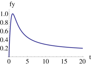
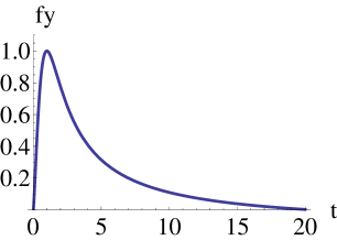
Figure 1: The plots of the torsion function $f_{y}$ in (6.6a): $8\mu^{2}\ell^{2}/\rho=-1$, $f_{y}[1]=1,f^{\prime}_{y}[1]=0$ (left), and in (6.6d): $f_{y}[1]=1,f^{\prime}_{y}[1]=0$ (right).

In the above two cases (d1) and (d2), the forms of the corresponding torsion functions $f_{y}$ are illustrated in Figure 1.

7 Exponential solution

In this section, we start with

$$K_{x}=e^{x}f_{x}(y)\,,\qquad K_{y}=e^{x}f_{y}(y)\,,\qquad H=e^{x}h(y)\,,$$ (7.1)

whereupon the field equations (4.5) become:

$$(y^{2}+\rho y^{2}\partial_{yy}+2\mu^{2}\ell^{2})f_{x}+\bigl{[}(1-\rho)y^{2}\partial_{y}-(1+\rho)y\bigr{]}f_{y}=0\,,$$ (7.2a)

$$(y^{2}\partial_{yy}+\rho y^{2}+2\mu^{2}\ell^{2})f_{y}+\bigl{[}(1-\rho)y^{2}\partial_{y}+(1+\rho)y\bigr{]}f_{x}=0\,,$$ (7.2b)

$${\hat{S}}H=\sigma(yf_{x}+y\partial_{y}f_{y}-f_{y})\,,$$ (7.2c)

and ${\hat{S}}H=e^{x}\left[y(h+h^{\prime\prime})-2h^{\prime}\right]$.

As in the previous section, we assume that $H$ coincides with the vacuum solution of GR_Λ, defined by ${\hat{S}}H=0$. This imposes an extra condition on $f_{x}$ and $f_{y}$:

$$yf_{x}+y\partial_{y}f_{y}-f_{y}=0\quad\Rightarrow\quad\frac{f_{x}}{y}+\left(\frac{f_{y}}{y}\right)^{\prime}=0\,.$$ (7.3)

By introducing a change of variables, given by

$$f_{x}=yg_{x}\,,\quad f_{y}=yg_{y}\,,$$ (7.4a)

the condition (7.3) takes a simple form:

$$g_{x}+g^{\prime}_{y}=0\,.$$ (7.4b)

As a consequence, Eqs. (7.2a) and (7.2b) are transformed into

$$\rho y^{2}g_{y}^{(3)}+2\rho yg_{y}^{\prime\prime}+(\rho y^{2}+2\mu^{2}\ell^{2})g_{y}^{\prime}+2\rho yg_{y}=0\,,$$ (7.5a)

$$\rho y^{2}g_{y}^{\prime\prime}+(\rho y^{2}+2\mu^{2}\ell^{2})g_{y}=0\,.$$ (7.5b)

One can note that (7.5a) is equal to the derivative (with respect to $y$) of (7.5b). The solution of (7.5b) reads:

$$g_{y}=\sqrt{y}\bigl{[}D_{1}J_{\nu}(y)+D_{2}Y_{\nu}(y)\bigr{]}\,,$$ (7.6)

where $\nu=\frac{1}{2}\sqrt{1-8\mu^{2}\ell^{2}/\rho}$, and $J_{\nu}$, $Y_{\nu}$ are the Bessel functions of the first and second kind, respectively [17]. Hence:

$$f_{y}=y^{\frac{3}{2}}\left(D_{1}J_{\nu}(y)+D_{2}Y_{\nu}(y)\right)\,,$$ (7.7a)

and $$f_{x}=-yg^{\prime}_{y}$$ yields

$$f_{x}=\sqrt{y}\Bigl{[}D_{1}\Bigl{(}yJ_{\nu+1}(y)-(\nu+1/2)J_{\nu}(y)\Bigr{)}+D_{2}\Bigl{(}yY_{\nu+1}(y)-(\nu+1/2)Y_{\nu}(y)\Bigr{)}\Bigr{]}\,.$$ (7.7b)

The forms of the torsion functions (7.7) are illustrated in Figure 2.

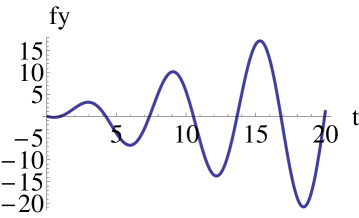
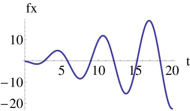
Figure 2: The plots of the torsion functions (7.7) for $D_{1}=D_{2}=1$, $8\mu^{2}\ell^{2}/\rho=-1$.

They are of the same type as the GR_Λ metric function $H_{3}$, defined in section 2. Together, they define our third specific Siklos wave with torsion.

8 Concluding remarks

In this paper, we introduced a new class of exact vacuum solutions of PGT, the Siklos waves with torsion. The solution is constructed in a way that respects the radiation nature of the original Siklos configuration in GR_Λ. This is achieved by an ansatz for the RC connection that produces only the tensorial irreducible mode of the torsion, propagating on the AdS background. A compact form of the PGT field equations is used to find three particular vacuum solutions belonging to the class of Siklos waves with torsion; they generalize the Kaigorodov, the homogeneous and the exponential solution of GR_Λ.

Appendix A Irreducible decomposition of the field strengths

We present here formulas for the irreducible decomposition of torsion and curvature in 4D Riemann–Cartan spacetime [5]; for general D, see [19].

It is convenient to start the exposition with the Bianchi identities:

$$\nabla T^{i}=R^{i}{{}_{m}}b^{m}\,,\qquad\nabla R^{ij}=0\,.$$ (A.1)

The torsion 2-form has three irreducible pieces:

$${}^{(2)}T^{i}=\frac{1}{3}b^{i}\wedge(h_{m}\,\hbox{\vrule height=0.0pt,width=4.0pt,depth=0.3pt\vrule height=7.0pt,width=0.3pt,depth=0.3pt\vrule height=0.0pt,width=2.0pt,depth=0.0pt}\hskip 0.8pt\,T^{m})\,,$$

$${}^{(3)}T^{i}=-\frac{1}{3}{{}^{\star}}\bigl{[}b^{i}\wedge{{}^{\star}}(T^{m}\wedge b_{m})\bigr{]}=\frac{1}{3}h^{i}\,\hbox{\vrule height=0.0pt,width=4.0pt,depth=0.3pt\vrule height=7.0pt,width=0.3pt,depth=0.3pt\vrule height=0.0pt,width=2.0pt,depth=0.0pt}\hskip 0.8pt\,(T^{m}\wedge b_{m})\,,$$

$${}^{(1)}T^{i}=T^{i}-{}^{(2)}T^{i}-{}^{(3)}T^{i}\,.$$ (A.2)

The RC curvature 2-form can be decomposed into six irreducible pieces:

$$\begin{array}[]{ll}{}^{(2)}R^{ij}=-{}^{*}(b^{[i}\wedge\Psi^{j]})\,,&{}^{(4)}R^{ij}=b^{[i}\wedge\Phi^{j]}\,,\\ {}^{(3)}R^{ij}=-\displaystyle\frac{1}{12}X\,{}^{*}(b^{i}\wedge b^{j})\,,&{}^{(6)}R^{ij}=\displaystyle\frac{1}{12}Wb^{i}\wedge b^{j}\,,\\ {}^{(5)}R^{ij}=\displaystyle\frac{1}{2}b^{[i}\wedge h^{j]}\,\hbox{\vrule height=0.0pt,width=4.0pt,depth=0.3pt\vrule height=7.0pt,width=0.3pt,depth=0.3pt\vrule height=0.0pt,width=2.0pt,depth=0.0pt}\hskip 0.8pt\,(b^{m}\wedge W_{m})\,,&{}^{(1)}R^{ij}=R^{ij}-\sum_{a=2}^{6}{}^{(a)}R^{ij}\,.\end{array}$$

where

$$W^{i}:=h_{m}\,\hbox{\vrule height=0.0pt,width=4.0pt,depth=0.3pt\vrule height=7.0pt,width=0.3pt,depth=0.3pt\vrule height=0.0pt,width=2.0pt,depth=0.0pt}\hskip 0.8pt\,R^{mi}={Ric}^{i}\,,\qquad W:=h_{i}\,\hbox{\vrule height=0.0pt,width=4.0pt,depth=0.3pt\vrule height=7.0pt,width=0.3pt,depth=0.3pt\vrule height=0.0pt,width=2.0pt,depth=0.0pt}\hskip 0.8pt\,W^{i}=R\,,$$

$$X^{i}:={}^{*}(R^{ki}\wedge b_{k})\,,\qquad X:=h_{i}\,\hbox{\vrule height=0.0pt,width=4.0pt,depth=0.3pt\vrule height=7.0pt,width=0.3pt,depth=0.3pt\vrule height=0.0pt,width=2.0pt,depth=0.0pt}\hskip 0.8pt\,X^{i}\,.$$ (A.3)

and

$$\Phi_{i}:=W_{i}-\frac{1}{4}b_{i}W-\frac{1}{2}h_{i}\,\hbox{\vrule height=0.0pt,width=4.0pt,depth=0.3pt\vrule height=7.0pt,width=0.3pt,depth=0.3pt\vrule height=0.0pt,width=2.0pt,depth=0.0pt}\hskip 0.8pt\,(b^{m}\wedge W_{m})\,,$$

$$\Psi_{i}:=X_{i}-\frac{1}{4}b_{i}X-\frac{1}{2}h_{i}\,\hbox{\vrule height=0.0pt,width=4.0pt,depth=0.3pt\vrule height=7.0pt,width=0.3pt,depth=0.3pt\vrule height=0.0pt,width=2.0pt,depth=0.0pt}\hskip 0.8pt\,(b^{m}\wedge X_{m})\,.$$ (A.4)

The trace and symmetry properties of ${}^{(n)}R_{ij}$ can be found in Ref. [19], p. 127. All these properties are satisfied by our ansatz.

For torsion-free solutions, the first Bianchi identity in (A.1) implies $X^{i}=0$, hence ${}^{(2)}R^{ij}$ and ${}^{(3)}R^{ij}$ vanish. Moreover, ${Ric}_{[ij]}=0$ implies ${}^{(5)}R^{ij}=0$. The remaining three curvature parts, 1-st, 4-th and 6-th, are the PGT analogues of the irreducible pieces of the Riemannian curvature. In Riemannian geometry, ${}^{(1)}R^{ij}$ coincides with the Weyl (conformal) tensor,

$$C^{ij}:=R^{ij}-\frac{1}{2}(b^{i}{Ric}^{j}-b^{j}{Ric}^{i})+\frac{1}{6}Rb^{i}b^{j}\,,$$

but in the RC geometry, ${}^{(1)}R^{ij}$ differs from $C^{ij}$ by the presence of torsion terms. Thus, ${}^{(1)}R^{ij}$ is a true extension of $C^{ij}$ to the RC geometry. The 4-th component is defined in terms of the symmetric traceless Ricci tensor,

$$\Phi_{i}=\left({Ric}_{(ij)}-\frac{1}{4}\eta_{ij}R\right)b^{j}\,.$$ (A.5)

The above formulas are taken from Refs. [5, 19] with one modification: the definition of $W^{i}$ is taken with an additional minus sign (Landau–Lifshitz convention), and for consistency, the overall signs of the 4th, 5th and 6th curvature parts are also changed.

Appendix B PGT field equations

The gravitational dynamics of PGT is determined by a Lagrangian $L_{G}=L_{G}(b^{i},T^{i},R^{ij})$ (4-form), which is assumed to be at most quadratic in the field strengths (quadratic PGT) and parity invariant. The form of $L_{G}$ can be conveniently represented as

$$L_{G}=-{{}^{\star}}(a_{0}R+2{\mit\Lambda})+\frac{1}{2}T^{i}H_{i}+\frac{1}{4}R^{ij}H^{\prime}_{ij}\,,$$ (B.1)

where $H_{i}:=\partial L_{G}/\partial T^{i}$ (the covariant momentum) and $H^{\prime}_{ij}$ define the quadratic terms in $L_{G}$:

$$H_{i}=2\sum_{n=1}^{3}{{}^{\star}}(a_{n}{}^{(n)}T_{i})\,,\qquad H^{\prime}_{ij}:=2\sum_{n=1}^{6}{{}^{\star}}(b_{n}{}^{(n)}R_{ij})\,.$$ (B.2a)

Varying $$L_{G} b^{i} \omega^{ij} H_{ij}:=\partial L_{G}/\partial R^{ij}$$ with respect to and yields the PGT field equations in vacuum. After introducing the complete covariant momentum by

$$H_{ij}=-2a_{0}{{}^{\star}}(b^{i}b^{j})+H^{\prime}_{ij}\,,$$ (B.2b)

these equations can be written in a compact form as

$$(1ST) \nabla H_{i}+E_{i}=0\,,$$

$$(2ND) \nabla H_{ij}+E_{ij}=0\,,$$ (B.3)

where $E_{i}$ and $E_{ij}$ are the gravitational energy-momentum and spin currents:

$$E_{i}:=h_{i}\,\hbox{\vrule height=0.0pt,width=4.0pt,depth=0.3pt\vrule height=7.0pt,width=0.3pt,depth=0.3pt\vrule height=0.0pt,width=2.0pt,depth=0.0pt}\hskip 0.8pt\,L_{G}-(h_{i}\,\hbox{\vrule height=0.0pt,width=4.0pt,depth=0.3pt\vrule height=7.0pt,width=0.3pt,depth=0.3pt\vrule height=0.0pt,width=2.0pt,depth=0.0pt}\hskip 0.8pt\,T^{m})H_{m}-\frac{1}{2}(h_{i}\,\hbox{\vrule height=0.0pt,width=4.0pt,depth=0.3pt\vrule height=7.0pt,width=0.3pt,depth=0.3pt\vrule height=0.0pt,width=2.0pt,depth=0.0pt}\hskip 0.8pt\,R^{mn})H_{mn}\,,$$

$$E_{ij}:=-(b_{i}H_{j}-b_{j}H_{i})\,.$$ (B.4)

The general field equations (B.3) are used in section 4 to describe specific dynamical aspects of the Siklos waves with torsion. In the Riemannian sector with $T^{i}=0$, we have $H_{i}=0$ and $E_{ij}=0$, and the field equations (B.3) reduce to the form given in section 3.

References

• [1] H. Weyl, Elektron and Gravitation I (in German), Zeitschrift f. Physik, 56, 330–352 (1929); translated in L. O’Raifeartaigh, The Dawning of Gauge Theory (Princeton Univ. Press, Princeton, 1997).
• [2] C. N. Yang and R. Mills, Conservation of isotopic spin and isotopic gauge invariance, Phys. Rev. 96, 191–195 (1954).
• [3] R. Utiyama, Invariant theoretical interpretation of interactions, Phys. Rev. 101, 1597–1607 (1956).
• [4] T. W. B. Kibble, Lorentz invariance and the gravitational field, J. Math. Phys. 2, 212–221 (1961);
D. W. Sciama, On the analogy between charge and spin in general relativity, in: Recent Developments in General Relativity, Festschrift for Infeld (Pergamon Press, Oxford; PWN, Warsaw, 1962) pp. 415–439.
• [5] Yu. N. Obukhov, Poincaré gauge gravity: Selected topics, Int. J. Geom. Meth. Mod. Phys. 3, 95–138 (2006).
• [6] M. Blagojević and F. W. Hehl (eds.), Gauge Theories of Gravitation, A Reader with Commentaries (Imperial College Press, London, 2013).
• [7] J. Ehlers and W. Kundt, Exact solutions of the gravitational field equations, in: Gravitation: an Introduction to Current Research, ed. L. Witten (Willey, New York, 1962) pp. 49–101.
• [8] V. Zakharov, Gravitational Waves in Einstein’s Theory (Halsted Press, New York, 1973).
• [9] H. Stephani, D. Kramer, MacCallum, C. Hoenselaers, and E. Herlt, Exact Solutions of Einstein s Field Equations, 2nd ed. (Cambridge University Press, Cambridge, 2003).
• [10] J.B. Griffiths and J. Podolský, Exact Space-Times in Einstein’s General Relativity, (Cambridge University Press, Cambridge, 2009).
• [11] W. Adamowicz, Plane waves in gauge theories of gravitation, Gen. Rel. Grav. 12, 677–691 (1980);
P. Singh and J. B. Griffiths, A new class of exact solutions of the vacuum quadratic Poincar e gauge field theory, Gen. Rel. Grav. 22, 947–956 (1990);
V. V. Zhytnikov, Wavelike exact solutions of $R+R^{2}+Q^{2}$ gravity, J. Math. Phys. 35, 6001–6017 (1994);
M.-K. Chen, D.-C. Chern, R.-R. Hsu, and W. B. Yeung, Plane-fronted torsion waves in a gravitational gauge theory with a quadratic Lagrangian, Phys. Rev. D 28, 2094–2095 (1983);
O. V. Babourova, B. N. Frolov and E. A. Klimova, Plane torsion waves in quadratic gravitational theories, Class. Quant. Grav. 16, 1149–1162 (1999);
A. D. King and D. Vassiliev, Torsion waves in metric-affine field theory, Class. Quantum Grav. 18, 2317–2329 (2001);
V. Pasić and D. Vassiliev, PP-waves with torsion and metric-affine gravity, Class. Quant. Grav. 22, 3961–3976 (2005).
• [12] S. T. C. Siklos, Lobatchevsky plane gravitational waves, in: Galaxies, Axisymmetric Systems and Relativity, ed. M. A. H. MacCallum (Cambridge University Press, Cambridge, 1985) pp. 247–274.
• [13] M. Blagojević and B. Cvetković, Siklos waves with torsion in 3D, JHEP 11, 141 (2014) [16 pages].
• [14] J. Podolský, Interpretation of the Siklos solutions as exact gravitational waves in the anti-de Sitter universe, Class. Quant. Grav. 15, 719–733 (1998).
• [15] J. Podolský, Exact nonsingular waves in the Anti-de Sitter universe, Gen. Rel. Grav. 33, 1093–1113 (2001).
• [16] The field equations (4.4) for the Siklos waves with torsion are checked using the Excalc package of the computer algebra system Reduce; after being transformed to the form (4.5), they are solved with the help of Wolfram Mathematica.
• [17] Pocketbook of Mathematical Functions, abridged edition of Handbook of Mathematical Functions, M. Abramowitz and I. Stegun (eds.), material selected by M. Danos and F. Rafelski (Verlag Harri Deutsch, Frankfurt am Mein, FRG, 1984); chapters 9 (Bessel functions) and 15 (hypergeometric functions);
A. Erdélyi, W. Magnus, F. Oberhettinger, and F. G. Tricomi, Higher Transcendental Functions, Vol. 1 (McGraw-Hill, New York, 1953); chapter 5 (Meijer’s G function).
• [18] K. Hayashi and T. Shirafuji, Gravity from Poincaré Gauge Theory of the Fundamental Particles. I, Prog. Theor. Phys. 64 866–882 (1980).
• [19] F. W. Hehl, J. D. McCrea, E.W. Mielke, and Y. Ne eman, Metric-affine gauge theory of gravity: Field equations, Noether identities, world spinors, and breaking of dilation invariance, Phys. Rept. 258, 1–171 (1995).