A Twenty Year Decline in Solar Photospheric Magnetic Fields: Inner-Heliospheric Signatures and Possible Implications?

Abstract

We report observations of a steady 20 year decline of solar photospheric fields at latitudes $\geq$45^o starting from $\sim$1995. This prolonged and continuing decline, combined with the fact that Cycle 24 is already past its peak, implies that magnetic fields are likely to continue to decline until $\sim$2020, the expected minimum of the ongoing solar Cycle 24. In addition, interplanetary scintillation (IPS) observations of the inner heliosphere for the period 1983–2013 and in the distance range 0.2–0.8 AU, have also shown a similar and steady decline in solar wind micro-turbulence levels, in sync with the declining photospheric fields. Using the correlation between the polar field and heliospheric magnetic field (HMF) at solar minimum, we have estimated the value of the HMF in 2020 to be 3.9 ($\pm$0.6) and a floor value of the HMF of $\sim$3.2 ($\pm$0.4) nT. Given this floor value for the HMF, our analysis suggests that the estimated peak sunspot number for solar Cycle 25 is likely to be $\sim$ 62 ($\pm$12).

JANARDHAN ET AL. Photospheric Fields: A 20 year Decline Corresponding author:P. Janardhan, Astronomy & Astrophysics Division, Physical Research Laboratory, Ahmedabad 380009, India. (e-mail: jerry@prl.res.in)

1 Introduction

Sunspots or dark regions of strong magnetic fields on the Sun are generated via magneto-hydrodynamic processes involving the cyclic generation of toroidal, sunspot fields from pre-existing poloidal fields and their eventual regeneration through a process, referred to as the solar dynamo. This leads to the well known periodic 11-year solar cycle with sunspot numbers climbing, at solar maximum, up to 200 in very active or strong solar cycles and dropping down, at solar minimum, to 20 or less sunspots during periods of solar minimum.

The current solar Cycle 24, on the one hand, was preceded by one of the deepest solar minima experienced in the past 100 years causing Cycle 24 to not only start $\sim$1.3 years later than expected (Jian et al., 2011), but also be the weakest since solar Cycle 14 in the early 1900’s. With a peak smoothed monthly sunspot number $\sim$75 in November 2013, the maximum of solar Cycle 24 has in fact been dubbed the “mini” solar maximum (McComas et al., 2013). On the other hand, measurements of the sunspot umbral field strength have been shown to be steadily decreasing by $\sim$50 G per year since $\sim$1998 (Penn and Livingston, 2006; Livingston et al., 2012). Also the sunspot formation fraction, the ratio of the observed monthly smoothed sunspot number (SSN) and the SSN value derived from the monthly F10.7cm radio flux, have been reported to be steadily decreasing since $\sim$1995 (Livingston et al., 2012). It is important to bear in mind that for field strengths below about 1500 G, there will be no contrast between the photosphere and sunspot regions (Livingston et al., 2012), thereby making sunspots invisible. These authors have claimed that the umbral field strengths in Cycle 25 would be around 1500 G, and thus, there would be very little/no sunspots visible on the solar photosphere in the next solar Cycle 25. Studies of the heliospheric magnetic field (HMF), using ${\sl{in-situ}}$ measurements at 1 AU, have also shown a significant decline in strength (Smith and Balogh, 2008; Wang et al., 2009; Connick et al., 2011; Cliver and Ling, 2011). It has been reported that during the so called “mini” maximum of Cycle 24, the HMF intensity was more like that during the minimum of Cycle 23 recording an all-time-low space age value.

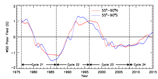
Figure 1: The polar cap fields derived from the Wilcox Solar Observatory (WSO) data for the Northern (red) and Southern (blue) hemispheres for the period 1976.42 – 2014.91, covering solar cycles 21, 22, 23 and 24. The Southern hemisphere fields have been inverted for ease of comparison.

Recent studies, using synoptic magnetograms from the National Solar Observatory (NSO), Kitt-Peak (NSO/KP), USA, have reported a steady decline in photospheric magnetic fields at helio-latitudes ${\geq{45^{\circ}}}$, with the observed decline having begun in the mid-1990’s (Janardhan et al., 2010). Using 327 MHz observations from the four station IPS observatory of the Solar-Terrestrial Environment Laboratory (STEL), Nagoya University, Japan, we have examined solar wind micro-turbulence levels in the inner-heliosphere and have found a similar steady decline, continuing for the past 18 years, and in sync with the declining photospheric fields (Janardhan et al., 2011). Our present work has confirmed that this declining trend is continuing to the present. A study, covering solar Cycle 23, of the solar wind density modulation index, $\epsilon_{N}\equiv\Delta{N}/N$, where, $\Delta{N}$ is the rms electron density fluctuations in the solar wind and N is the density, has reported a decline of around 8% in the distance range 0.2 AU to 0.8AU (Bisoi et al., 2014a). This decline has been attributed by the authors to the steadily declining solar photospheric fields. In light of the very unusual nature of the minimum of solar Cycle 23 and the current very weak solar Cycle 24, we have re-examined in this paper, both solar photospheric magnetic fields and the HMF for the period 1975 – 2014 and solar wind micro-turbulence levels during 1983 – 2013.

The aim of this paper is to try and estimate the maximum strength of solar Cycle 25 and address the question of whether we are headed towards a long period of little/no sunspot activity similar to the well known Maunder minimum (1645-1715 AD) when the sunspot activity was extremely low.

2 Data

2.1 Magnetic Field

Magnetic field measurements from ground based magnetograms are freely available in the public domain and we have made use of these observations in this paper for estimating solar magnetic fields. We have used photospheric magnetic fields from the Wilcox Solar Observatory (WSO), the National Solar Observatory at Kitt Peak, USA (NSO/KP), and the Synoptic Long-term Investigation of the Sun (SOLIS) facility at Kitt Peak, USA (NSO/SOLIS). For estimating polar fields at latitudes from 55^∘ – 90^∘, we have used data obtained from the Wilcox Solar Observatory (WSO)(http://wso.stanford.edu/Polar.html), covering the period from 31 May 1976 (1976.42) – 28 Nov 2014 (2014.91). The polar field strength at WSO are line-of-sight magnetic fields measured each day in the polemost apertures for the Northern and Southern solar hemispheres calculated for every 10 days. A 20 nHz low pass filter is used to remove the yearly projection effects from the measured line-of-sight magnetic fields. For the estimation of photospheric fields in the latitude range 0^∘ – 45^∘ and 45^∘ – 78^∘, synoptic magnetograms were used from NSO/KP (ftp://nsokp.nso.edu/kpvt/synoptic/mag/) and NSO/SOLIS (ftp://solis.nso.edu/synoptic/level3/vsm/merged/carr-rot/), respectively. The data are available as standard FITS files in the longitude and latitude format of 360 $\times$ 180 arrays, for the period February 1975 (1975.14) – July 2014 (2014.42), covering Carrington Rotations (CR) CR1625 – CR2151.

For the study of heliospheric magnetic fields (HMF), we have used 27-day averaged HMF data at 1 AU, available in the public domain from the OMNI2 database, for the period 1975 – 2014. The OMNI data base is a compilation of hourly-averaged, near-Earth solar wind magnetic field and plasma parameter data from several spacecraft in geocentric or L1 (Lagrange point) orbits.

2.2 IPS measurements

For the study of solar wind micro-turbulence levels in the inner heliosphere, we have used the daily IPS measurements of scintillation indices, spanning the period from 1983 to 2013. The IPS observations on a set of about 200 chosen extra-galactic radio sources have been carried out on a regular basis at the multi-station IPS observatory of STEL, Japan to determine scintillation indices at 327 MHz (Kojima and Kakinuma, 1990; Asai et al., 1998) since 1983 till date. Prior to 1994, however, these observations were carried out only by the three-station IPS facility at Toyokawa, Fuji, and Sugadaira. One more antenna was commissioned at Kiso in 1994, forming a four – station dedicated IPS network, that has been making systematic and reliable estimates scintillation indices (Tokumaru et al., 2012). Each day about a dozen selected radio sources have been observed such that each source would have been observed over the whole range of heliocentric distances between 0.2 and 0.8 AU in a period of about 1 year.

3 Photospheric Magnetic Fields

While studying solar polar fields, different groups of researchers have considered different solar latitude ranges to represent solar high latitude fields or polar fields, by averaging the magnetic flux in the defined high latitude polar regions. Till date the polar area considered has been arbitrary (Upton and Hathaway, 2014). For example, Wilcox Solar Observatory (WSO) polar fields are those at latitudes $\geq$55^∘. Other researchers have used the area above latitudes $\geq$60^∘ (de Toma, 2011) and still others have used the area above latitudes $\geq$70^∘ (Muñoz-Jaramillo et al., 2012) to represent polar or high latitude fields.

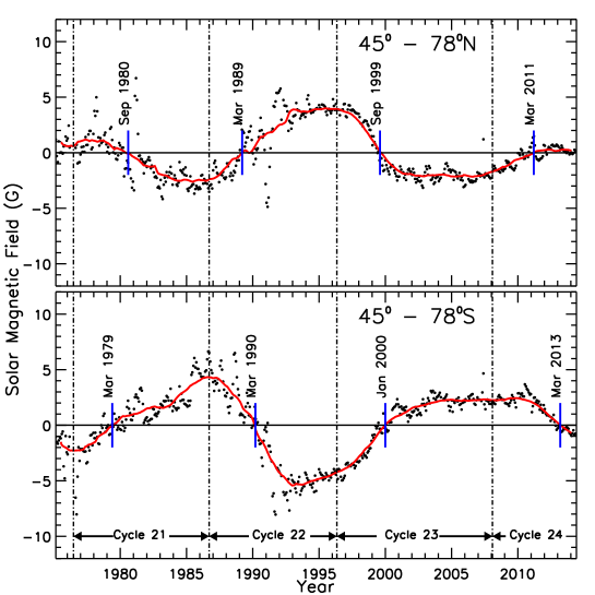
Figure 2: The signed photospheric magnetic fields in the latitude range 45^∘ to 78^∘ for the Northern (top) and Southern (bottom) hemispheres for solar cycles 21, 22, 23 and 24. The solid black dots are actual magnetic measurements from the NSO/KP magnetograms, while the solid red curve depicts the smoothed magnetic fields. The time of reversal of magnetic fields for each Solar Cycle in both the hemispheres is indicated by a small blue arrow.

For the present study, we have considered photospheric magnetic fields in the latitude range 45^∘ – 78^∘ as representative of polar fields, referred to in the rest of the paper as high-latitude fields. Using NSO/KP data, available in the public domain as described earlier, photospheric magnetic fields were estimated by a longitudinal average of the whole 360^∘ array of longitude to produce 1^∘ strips of data for each CR of 27.275 days. High-latitude fields were then computed by appropriate averaging (Janardhan et al., 2010; Bisoi et al., 2014b).

It is known that the (signed) polar field or polar flux normally reverses polarity at each solar maximum, commonly referred to as “polar field reversals or polar reversals” (Babcock, 1959, 1961). For example, if the polar field in the Northern (Southern) hemisphere has positive (negative) polarity, then after polar reversal it will have negative (positive) polarity. The solar polar fields reverse because the excess amount of trailing polarity flux from decaying sunspots move polewards, cancel the polar cap fields of opposite polarity, and impart a new polarity. It has been seen however, that the reversal is hemispherically asymmetric or in other words, occurs at different times in the Northern and Southern hemispheres (Svalgaard and Kamide, 2013). Figure 1 shows the signed polar cap fields derived from WSO data for the Northern (red) and Southern (blue) solar hemisphere with the Southern polar cap fields being inverted for ease of comparison. The hemispherical asymmetry in the polar field reversals in each solar hemisphere for solar cycles 21, 22, 23 and 24, in the latitude range 45^∘ – 78^∘, is clearly seen from Fig. 1.

The upper and lower panel of Figure 2 shows the signed value of the high-latitude fields for the solar Northern and Southern hemispheres respectively, for solar cycles 21, 22, 23, and 24. The solid black dots are actual magnetic measurements derived using NSO/KP magnetograms, while the solid red curve shows the variation of the smoothed magnetic fields. A field reversal is deemed to have taken place when the solid red curve in Fig. 2 changes sign. The small blue lines in both panels of Fig. 2 indicate the times of field reversal in each solar hemisphere. It is however difficult to define the exact moment of reversal as the timing of reversal depends on the selection of polar area (Upton and Hathaway, 2014). Both the reversal of magnetic fields, in the latitude range 45^∘ – 78^∘, and the asymmetry in the reversal between the two hemispheres is evident from Figure 2. It can be seen that the time difference in the reversal is of around one year for Cycles 21–23, while it was unusually large and around two years for Cycle 24, with the reversal in the North having occurred in March 2011, and the reversal in the South having taken place in March 2013.

The hemispheric asymmetry of polar reversal has been primarily attributed to the hemispheric asymmetry of solar activity (Svalgaard and Kamide, 2013) itself. Figure 3 shows the variation of toroidal or sunspot fields for solar cycles 21, 22, 23, and 24 in the latitude range 0^∘ – 45^∘. These fields were estimated from NSO/KP magnetograms as described by Janardhan et al. (2010). From Figure 3, it is clear that for Cycle 24, the Southern hemisphere reached its activity peak $\sim$2 years after the Northern hemisphere. This hemispheric asymmetry in solar activity has presumably led to the observed two year difference in the times of field reversals between the two solar hemispheres in Cycle 24. In addition, it may be noted that the occurrence of magnetic field reversal in both the hemispheres in Cycle 24 (see Fig. 1 and Fig. 2) indicates that the ongoing solar Cycle 24 is around or past its peak and that the declining phase of the cycle has begun.

It is clear from Figure 2 that the high latitude fields in Cycle 24 are comparatively weaker than in Cycles 22 and 23. However, it is the unsigned (absolute) high-latitude photospheric field strengths, as shown in Figure 4, which showed a remarkable and steady decrease for $\sim$20 years, starting from $\sim$1995. The small filled black circles in Fig. 4 represent the unsigned high latitude fields estimated from NSO/KP magnetograms as described by Janardhan et al. (2010). The large open blue circles in Fig. 4 are annual means of the data with 1$\sigma$ error bars. The declining trend in the field strength is seen to continue after the slight increase during the period 2010 – 2011 and the annual means for these two years have been shown by large open black circles. The vertical dotted lines in Fig. 4 are drawn at solar maximum for each of the 4 cycles 21, 22, 23 and 24. An inspection of the behaviour of the annual means in Cycles 21, 22, and 23 indicate that the field strength normally declines, as expected, after the solar maximum until the solar minimum. The fact that polar field reversals have taken place in both solar hemispheres in Cycle 24 (see Fig. 2) implies that Cycle 24 is now past its maximum and into its declining phase. As a result, the declining trend in the field strength will continue at least until 2020, the expected minimum of the current Cycle 24. The solid red line in Fig. 4 is a linear fit to the annual means for the period 1994.48  –  2014.42, while the dotted red line is a linear extrapolation of the best fit line until 2020. It must be noted that the linear fit used is a least-squares fit to the annual means (open blue and black circles in Fig.4), and not to the actual magnetic measurements (black filled circles in Fig. 4). The solid black line in Fig. 4 is a linear fit to the annual means after leaving out the two annual means (black open circles in Fig. 4) which showed a deviation from the declining trend, in 2010 and 2011. The dotted black line is a linear extrapolation to 2020, the expected minimum of the ongoing Cycle 24.

The two least square fits shown in Fig. 4 are both statistically significant with a Pearson’ correlation coefficient of r=-0.91, at a significance level of 99% (red solid line) and r = -0.98, at a significance level of 99%(black solid line). Thus, the steady decline which started in $\sim$1995 is expected to go on until 2020, (the expected minimum of Cycle 24) that is, for a period of $\sim$ 25 years starting from 1995. From the extrapolation of the two best fit lines, the expected field strength in 2020 can be determined. The field strength will drop to $\sim$1.8 $\pm$ 0.08 G by 2020 if we consider the fit, in Fig. 4, for the annual means represented by

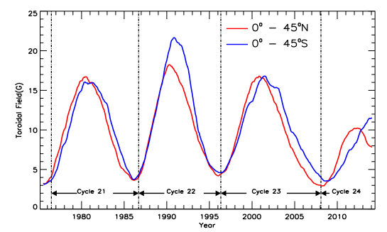
Figure 3: The toroidal field in the Northern (red) and Southern (blue) hemispheres for solar cycles 21, 22, 23 and 24, obtained using NSO/KP magnetic measurements.

the fitted red line and it will drop to $\sim$1.4 $\pm$ 0.04 G, for the annual means represented by the fitted black line. The two dashed horizontal lines in Fig. 4 are marked at 1.4 G and 1.8 G and represent respectively, the expected field strength in 2020 as derived from the linear extrapolation of the black straight line fit, which excludes the two annual means in 2010 and 2011 and the red straight line fit, which does not exclude the annual means in 2010 and 2011.

It must be noted that our study of photospheric fields, showing a steady decline in the absolute value of the field strength for $\sim$ 20 years, are confined to the high latitudes ($\geq$ 45^∘), where sunspots are not present. However, the high-latitude (polar) field and the toroidal field are strongly linked through the solar dynamo that causes the waxing and waning of the solar cycle with a period of 11 years (Charbonneau, 2010). Solar dynamo models assume that the Sun’s pre-existing poloidal field is transformed to a toroidal field within the Sun, and appear as sunspots at the start of the each new cycle. It is also known that the Sun’s polar field serves as a seed for future solar activity through their transportation by an equatorward subsurface meridional flow (Petrie, 2012) from the pole to the equator. As a result, polar fields are an important and crucial input in predicting the strength of future solar cycles (Schatten and Pesnell, 1993; Schatten, 2005; Svalgaard et al., 2005; Choudhuri et al., 2007). In the following section, we have used the high-latitude fields at the cycle minimum to predict the sunspot number at the solar maximum of the next cycle.

As mentioned earlier, since the Cycle 24 is already past its peak, the field strength is expected to decline until 2020, the minimum of Cycle 24. Such continuously weak high-latitude fields would imply that the toroidal field strengths will be also weak and produce weak sunspot fields in subsequent cycles.

4 The Heliospheric Magnetic Field

The floor level of the HMF is basically the yearly average value to which the HMF strength returns to, or approaches, at each solar minimum. A floor level of the HMF exists due to the constant baseline flux from the slow solar wind, and implies the presence of magnetized solar wind even in the absence (near-absence) of sunspot activity and polar fields. Since small-scale magnetic fields on the Sun are thought to be the source of slow solar wind flows they basically determine the floor (Cliver and Ling, 2011). In a study of heliospheric magnetic fields (HMF) from 1872 – 2004, Svalgaard and Cliver (2007) had proposed a floor level for the HMF of 4.6 nT. In subsequent studies however, measurements of the HMF at 1 AU, have shown a significant decline in their strength (Smith and Balogh, 2008; Wang et al., 2009; Connick et al., 2011; Cliver and Ling, 2011), going well below 4.6 nT during the minimum of Solar Cycle 23. Figure 5 shows (filled black circles) measurements of the 27-day averaged values of HMF and (open blue circles) annual means of HMF with 1 sigma error bars between 1975 – 2014, obtained using OMNI2 data at 1 AU. The horizontal dotted line is marked at the proposed floor value of the HMF of 4.6 nT (Svalgaard and Cliver, 2007), while the monthly averaged sunspot number, scaled down (for convenience) by a factor of 10 (SSN/10) from NOAA Geophysical Data Center is shown by the solid black curve with the smoothed value overplotted in red. The vertical grey bands demarcate 1 year intervals (Wang et al., 2009) around the minima of solar cycles 20, 21, 22 and 23 corresponding to CR1642–1654, CR1771–1783, CR1905–1917, and CR2072–2084, respectively. Average values of the high latitude (45^∘ – 78^∘) fields were computed in these 1 year intervals for the period 1975 – 2014 using NSO/KP synoptic magnetograms. The use of these averages will be described subsequently.

It is evident from Figure 5 that the HMF has declined well below the proposed floor level of 4.6 nT, and has reached $\sim$3.5 nT during the minimum of Cycle 23. Due to the decline of the HMF below 4.6 nT, Cliver and Ling (2011) used the dipole magnetic moment derived from polar magnetic field measurements of the Wilcox Solar Observatory (WSO) to revise the floor level using two independent methods. The first was by using a correlation between the dipole moment and the HMF at Cycle minimum, while the second was by using a correlation between the HMF at each Cycle minimum and the yearly sunspot number at Cycle maximum. These authors reported a revised floor level of 2.8 nT (Cliver and Ling, 2011). Using a calibrated database (data from MDI, WSO, and Mount Wilson Observatory (MWO) of polar magnetic flux and the HMF from OMNI, Muñoz-Jaramillo et al. (2012) have also reported the floor level of HMF of 2.77 nT.

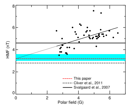
Figure 6: A plot of the polar field ($B_{p}$) as a function of the HMF for values during 1 year intervals around the minima of Cycles 20, 21, 22 and 23. A linear correlation between these two parameters, with a correlation coefficient of r=0.54, is shown and gives an intercept of 3.2 nT for $B_{r}$ when $B_{p}$ =0. The solid black and dashed black horizontal lines indicate the floor levels of the HMF of 4.6 nT, and 2.8 nT respectively, as derived by other researchers as described in the text, while dotted red line is marked at a floor of 3.2 nT derived from the present work. The blue band shows the range for our derived floor value of 3.2 nT.

We have revisited the floor level in the HMF using high latitude photospheric fields and the HMF from OMNI2 database. It is to be borne in mind that the aforementioned studies for finding the floor of HMF are based on the use of the signed polar flux (or the dipole moment estimated from the signed polar fields), while our studies have used the unsigned high-latitude fields. The high-latitude fields were computed from NSO/KP synoptic magnetograms for the period 1975.14 – 2014.42 and covering Carrington Rotations (CR) CR1625  –  CR2151. Figure 6 shows the correlation between the high-latitude or polar field ($B_{p}$) and the HMF ($B_{r}$) obtained using values for both $B_{p}$ and $B_{r}$ for 1 year intervals around the minima of cycles 20, 21, 22 and 23 (demarcated in Figure 5 by grey vertical bands).

Based on studies of correlation between polar flux and HMF at solar minimum (Cliver and Ling, 2011; Muñoz-Jaramillo et al., 2012), and the fact that the surviving polar fields actually determine the floor level of the HMF (Wang and Sheeley, 2013), we performed a linear fit to find the floor of HMF using its correlation with high-latitude fields. It is to be noted that the latter showed a significant decline over the last 20 years. A linear least square fit to the data (Pearson’s correlation coefficient of r=0.54 at a significance level of 99% and Spearman’s correlation coefficient of r=0.50 at a significance level of $\geq$99%) gave a value of the HMF of $B_{r}$ = 3.2$\pm$0.4 nT, when $B_{p}$ = 0 as shown in equation 1.

$$B_{r}=(3.2\pm 0.4)+(0.43\pm 0.09)\times B_{p}$$ (1)

This implies that even if the polar field, $B_{p}$, drops to zero or to very low values, the HMF will persist at a floor level of $\sim$3.2$\pm$0.4 nT. The solid black horizontal line in Figure 6 is drawn at 4.6 nT, the floor level of the HMF proposed by Svalgaard and Cliver (2007), the dashed black line is marked at a floor level of the HMF of 2.8 nT proposed by Cliver and Ling (2011) while the dotted red line is marked at a floor of 3.2 nT derived in the present work. The blue band shows the range for our derived floor value of 3.2 nT. From Figure 4 it can be seen that the high latitude field drops to between 1.4$\pm$0.04 G to 1.8$\pm$0.08 G in 2020, the expected minimum of Cycle 24. The linear relation obtained between the polar field and the HMF (equation 1) implies that the HMF will drop to 3.9$\pm$0.6 nT by $\sim$2020. The errors of 0.6 was estimated using standard formula for propagation of errors.

A good correlation has been reported (see Fig. 2 of Cliver and Ling (2011)) between the peak values of sunspot numbers smoothed over 13-month period ($SSN_{max}$) and the HMF at solar cycle minimum given by

$$SSN_{max}=63.4\times B_{r}-184.7$$ (2)

Using our estimates of 3.9 nT for the HMF ($B_{r}$) at 2020, the expected Cycle 24 minimum in the above linear relationship of $SSN_{max}$ and $B_{r}$ of Cliver and Ling (2011), the $SSN_{max}$ in Cycle 25 can be estimated and is likely to be $\sim$ 62 with statistical error bars of $\pm$ 12 (the estimated standard error of the mean using values of peak sunspot numbers for cycles 14–24 from Cliver and Ling (2011)) which is similar with cycle 24 within uncertainties.

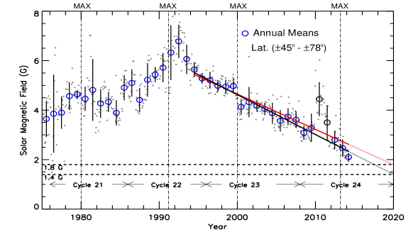
Figure 4: The photospheric magnetic fields in the latitude range 45^∘ – 78^∘, computed from the NSO/KP magnetograms, for the period of 1975.14 – 2014.42. While the solid filled dots are actual measurements of magnetic fields, the open large blue and black circles are annual means with 1$\sigma$ error bars. The solid red line is a best fit to the declining trend for all the annual means, while the solid black line is a best fit to the declining trend for the annual means after excluding the points of 2010 and 2011 (large black open circles). The dotted red and black lines are extrapolations of the two best fit lines until 2020, the expected minimum of the ongoing cycle 24. The horizontal dashed lines are marked at 1.8 G the expected field strength at 2020 from the red straight line fit and at 1.4 G, the expected field strength by 2020 from the black straight line fit. The vertical dotted lines are marked at the respective solar maximum of Cycles 21, 22, 23, and 24.

5 Solar Wind Micro-turbulence

It is known that photospheric fields during solar minimum conditions generally provide most of the heliospheric open flux (Solanki et al., 2000). At the solar minimum the high-latitude fields extend down to low latitudes into the corona and are then carried by the continuous solar wind flow to the interplanetary space to form the interplanetary magnetic field (IMF) (Schatten and Pesnell, 1993). So signatures of any change in the long term behaviour of photospheric fields are expected to be reflected in the IMF and solar wind. It has been shown (Ananthakrishnan et al., 1980) that solar wind micro-turbulence levels, as derived from IPS observations of the solar wind, are related to both rms electron density fluctuations and large-scale magnetic field

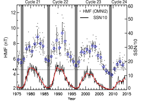
Figure 5: Measurements of the heliospheric magnetic field by solid black filled dots from OMNI2 data at 1 AU, obtained between 1975 – 2014, while open circles in blue are annual means with 1 sigma error bars. The monthly averaged sunspot number, scaled down by a factor of 10 is shown by the solid curve in black with the smoothed value overplotted in red. The horizontal line is marked at the floor level of the HMF of 4.6 nT proposed by Svalgaard et al., 2007. The vertical grey bands demarcate 1 year intervals around the minima of solar cycles 20, 21, 22 and 23.

fluctuations in fast solar wind streams. There is thus a likelihood of a definite causal relationship between the photospheric magnetic fields and micro-turbulence in the interplanetary medium thereby implying that a decrease in photospheric high-latitude fields will lead to a decrease in micro-turbulence levels in the solar wind.

IPS observations of compact extragalactic radio sources provide one with an effective and economical ground based method for probing the solar wind plasma in the inner-heliosphere both in and out of the ecliptic (Ananthakrishnan et al., 1995; Janardhan et al., 1997; Moran et al., 2000). IPS is a phenomenon in which coherent electromagnetic radiation from extragalactic radio sources passes through the turbulent, refracting solar wind, considered to be confined to a thin screen, and suffers scattering in that process. This results in random temporal variations of the signal intensity (scintillation) at the Earth (Hewish et al., 1964), which are modulated by the Fresnel filter function $\mathsf{Sin^{2}(\frac{q^{2}\lambda z}{4\pi})}$ where, q is the wave number of the irregularities, z is the distance from Earth to the screen, and $\lambda$ is the observing wavelength. Due to the action of the Fresnel filter, IPS observations are insensitive to larger scale solar wind density fluctuations caused by structures such as coronal mass ejections (CMEs). IPS observations thus enable one to probe solar wind electron density fluctuations of scale sizes from 10 to 100 km both in and out of the ecliptic (Pramesh Rao et al., 1974; Coles and Filice, 1985; Yamauchi et al., 1998; Fallows et al., 2008; Ananthakrishnan et al., 1995) and over a wide range of distances in the inner-heliosphere (Janardhan et al., 1996). In fact IPS is sensitive to very small changes in the rms electron density fluctuations ($\Delta$N) and has even been exploited to study the fine scale structure in cometary ion tails during radio source occultations by cometary tail plasma (Ananthakrishnan et al., 1975; Janardhan et al., 1991, 1992) and to study extremely low density events at 1 AU referred to as solar wind disappearance events, when the average solar wind densities at 1 AU dropped to less than 0.1 particles cm^-3 for extended periods of time (Balasubramanian et al., 2003; Janardhan et al., 2005, 2008a, 2008b).

The degree to which compact, point-like, extragalactic radio sources exhibit scintillation, as observed by ground-based radio telescopes, is quantified by the scintillation index (m) given by $\mathsf{m=\frac{{\Delta}S}{<S>}}$, where $\Delta$S is the scintillating flux and $<$S$>$ is the mean flux of the radio source being observed. For a given IPS observation, m is simply the root mean-square deviation of the signal intensity to the mean signal intensity and can be easily determined from the observed intensity fluctuations of compact extragalactic radio sources. Regular IPS observations to determine solar wind velocities and scintillation indices at 327 MHz (Kojima and Kakinuma, 1990; Asai et al., 1998) have been carried out since 1983 from the multi-station IPS observatory, at STEL, Japan.

For a typical IPS observation carried out at a wavelength $\lambda$, the line-of-sight to at extragalactic radio source passes through the solar wind at a distance ‘r’ defined as the perpendicular distance from the sun to the line-of-sight. This distance r (in AU) is given by Sin($\epsilon$) where, $\epsilon$ is the solar elongation (for a schematic of a typical IPS observation, see Figure 1 in Bisoi et al. (2014a)). Due to the movement of the Earth in its orbit by nearly one degree a day, daily observations of a given radio source over an extended period of time will therefore yield observations along different lines-of-sight at different distances from the sun thereby enabling one to probe the interplanetary medium over a large distance range r at meter wavelengths (Janardhan and Alurkar, 1993; Ananthakrishnan et al., 1995; Janardhan et al., 1996). For an ideal point-like radio source, m steadily increases with decreasing r or $\epsilon$ until it reaches a value of unity at some distance of the line-of-sight from the Sun. As r continues to decrease beyond this point, m will again drop off to values below unity. The distance beyond this ’turn-over’ can be effectively probed by IPS observations. For sources with extended angular diameters, in the range 10 to 500 milli arc second (mas), the measured m will be lower than the corresponding observation of a point source at a similar solar elongation. At an observing wavelength $\lambda$ of 92 cm or 327 MHz, r ranges from 0.2 to 0.8 AU in the inner-heliosphere and IPS is therefore an excellent, cost-effective, technique for studying the large-scale structure of the solar wind in the inner-heliosphere. In the present study, to examine the temporal evolution of m for a large number of sources, distributed around the sun both in and out of the ecliptic and observed systematically over a long period of time, it is necessary to remove both the distance dependence of m and the effect of source size to be able to intercompare observations. In brief, the distance dependence of m can be removed by dividing each observation of m, by the corresponding m of a point source observed at the same r as described in (Janardhan et al., 2011). Using many years of systematic IPS observations from the Ooty Radio Telescope (Swarup et al., 1971) at 327 MHz, Manoharan (2012) have established that the strongly scintillating radio source 1148-001 has an angular size $\sim$15 milli arc seconds (mas) while VLBI observations have reported an angular diameter of 10 mas (Venugopal et al., 1985). Thus, the radio source 1148-001 can be treated as an ideal point source and used to remove the distance dependence of m. A recent study of the temporal variations of scintillation index between 1983 – 2008, has reported a steady decline since $\sim$1995 (Janardhan et al., 2011).

Measurements of the scintillation index, m are basically a measure of the rms electron density fluctuations ($\Delta$N), or a proxy for the micro-turbulence in the solar wind. A global reduction in the long-term solar photospheric fields (Janardhan et al., 2010) would therefore reflect as a corresponding decline in the solar wind micro-turbulence levels, as inferred by these IPS measurements. Another recent study, covering the Solar Cycle 23, of the solar wind density modulation index, $\epsilon_{N}\equiv\Delta{N}/N$, where, $\Delta{N}$ is the rms electron density fluctuations in the solar wind and N is the density, reported a decline of around 8% (Bisoi et al., 2014a) from 1998 to 2008 which was attributed to the declining photospheric fields. We have therefore re-examined, using IPS observations from STEL, the solar wind micro-turbulence levels between 1983 – 2013 to see if the declining trend has been continuing after 2008.

The effect of the source size can be removed by the method as described in (Bisoi et al., 2014a). The theoretical values of m for radio sources of a given angular size as function of r can be computed using Marian’s coefficients assuming weak scattering and a power law distribution of density irregularities in the IP medium (Marians, 1975). For the observed values of m for each given source, the best fit Marians curve of a given source size was first determined. For example, the best fit Marians curve for 1148-001 corresponds to that obtained for a source size of 10 mas. The observed values of m for each source were then normalized by multiplying values of m at each r by a factor equal to the difference between the best fit Marians curve for the given source and the best fit Marians

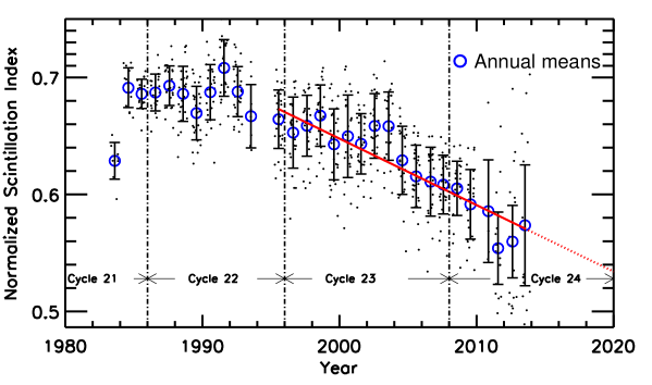
Figure 7: m as function of years for observations of 27 sources after making them both source size and distance independent. While the fine black dots show the actual measurements of m, the large blue open circles are annual means of m with 1 sigma error bars. The solid red line is a best fit to the declining trend while the dotted red line is an extrapolation of the fitted line upto 2020, indicated by a dashed vertical line.

curve for a point source at the corresponding r. Since 1148-001 is a good approximation to an ideal point source, for the present analysis, the observed m of all other sources were multiplied by a factor equal to the difference between the best fit Marians curve for the given source and the best fit Marians curve for 1148-001 (see Figure 3 in (Bisoi et al., 2014a) for full description).

After making all the observations of m both distance and source size independent, we shortlisted those sources for further analysis which had at least 400 observations distributed uniformly (with no significant data gaps) over the entire range of r spanning 0.2 to 0.8 AU. Using the criterion, we have finally shortlisted 26 sources from a group of around 200 sources. The source 1148-001 was included as the 27th source though it did not fully comply with the criterion (having few data gaps). Figure 7 shows, by fine black dots, the temporal variation of m for the 27 chosen sources with the large blue open circles representing annual means of m with 1 sigma error bars. It is evident that m continues to drop until the end of 2013. The solid red line in Fig. 7 is a best linear fit to the measurements of m for the period 1995 – 2013. Assuming that this declining trend seen in the normalized m continues, we have extrapolated the value of m until 2020, as indicated by a vertical red dashed line marked at 2020. The dotted red line is the extrapolation of the best fit line up to 2020. The steady reduction in the normalized m implies that by 2020, a 10 mas ‘point’ source like 1148-001, which is expected to show a normalized scintillation level close to unity will show the level of scintillation equivalent to that of a 160 mas source implying that that the solar wind micro-turbulence level has shown a significant reduction of approximately 30%.

6 Discussion and Conclusion

The present study, using synoptic magnetograms from the National Solar Observatory (NSO), Kitt-Peak (NSO/KP), USA, has shown a steady decline in photospheric magnetic fields at helio-latitudes ${\geq{45^{\circ}}}$, with the observed decline having begun in the mid-1990’s and continuing, to the end of the dataset through 2014. In addition, heliospheric micro-turbulence levels have also showed a steady decline in sync with the solar photospheric fields. The present, weak solar Cycle 24 coupled with the steady and continuing decline in high latitude photospheric fields, starting from $\sim$1995, therefore begs the question as to whether we are headed towards a so-called “grand minimum” (Usoskin et al., 2007) similar to the well known Maunder minimum (1645 – 1715 A.D.) when the sunspot activity was extremely low. There are studies that show that peak smoothed annual sunspot number prior to the onset of the Maunder minimum was around 50 (Eddy, 1976). A reconstruction of group sunspot numbers for the period 1392 – 1985 derived using ¹⁰Be ice core records from the North Greenland Icecore Project, reported a sunspot number, prior to the onset of the Maunder minimum, of around 60 (Inceoglu et al., 2014). Similarly, a reconstruction of decadal group sunspot numbers using ¹⁴C records from tree rings, shows a cycle averaged group sunspot number, prior to the onset of the Maunder minimum, of around 50 at 1610 A.D. (Usoskin et al., 2014). Vaquero et al. (2011) showed that the last cycle before the Maunder minimum was small, with sunspot number of about 20 suggesting for a gradual onset of the Maunder minimum.

Using ¹⁴C records from tree rings, sunspot numbers going back over the past 1000 solar cycles or $\sim$11000 years in time have been derived and 27 grand or prolonged solar minima, each lasting on average $\sim$6 – 7 solar cycles, have been identified in this data set (Usoskin et al., 2007). This implies that conditions in those, solar cycles, accounting for about 18% of the time, were such that they could force the Sun into grand minima. Choudhuri and Karak (2012) and Karak and Choudhuri (2013) gleaned very useful insights into the process of the onset of grand minima by showing how different characteristics of grand minima, seen in their $\sim$11000 year long data set, could be reproduced using a flux transport solar dynamo model. Their study has shown that gradual changes in meridional flow velocity lead to a gradual onset of grand minima while abrupt changes lead to an abrupt onset. In addition, these authors have reported that one or two solar cycles before the onset of grand minima, the cycle period tends to become longer. It is noteworthy that surface meridional flows over Cycle 23 (Hathaway and Rightmire, 2010) have shown gradual variations from 8.5 m s^-1 to 11.5 m s^-1 and 13.0 m s^-1 and Cycle 24 started $\sim$1.3 years later than expected. There is also evidence of longer cycles before the start of the Maunder and Spörer minimum (Miyahara et al., 2010). Modeling studies of the solar dynamo invoking meridional flow variations over a solar cycle have also successfully reproduced the characteristics of the unusual minimum of sunspot Cycle 23 and have shown that very deep minima are generally associated with weak polar fields (Nandy et al., 2011).

A recent analysis of yearly mean sunspot-number data covering the period 1700 to 2012 showed that it is a low-dimensional deterministic chaotic system (Zachilas and Gkana, 2015). Their model for sunspot numbers was able to successfully reconstruct the Maunder Minimum period and they were hence able to use it to make future predictions of sunspot numbers. Their study predicts that the level of future solar activity will be significantly decreased leading us to another prolonged or Maunder-like sunspot minimum that will last for several decades. Our study on the other hand, using an entirely different approach, also strongly suggests a similar long period of reduced solar activity.

Our analysis shows that both solar photospheric fields and solar wind micro-turbulence levels have been steadily declining from $\sim$1995 and that the trend will continue at least until the minimum of Cycle 24 in 2020. Based on the correlation between the high-latitude magnetic field and the HMF at the solar minima, we expect that the HMF will decline to a value of $\sim$3.9 ($\pm$0.6) nT by 2020. We also estimate that the peak 13 month smoothed sunspot number of Cycle 25 will be $\sim$62 $\pm$ 12, thereby making Cycle 25 a slightly weaker cycle than Cycle 24, and only a little stronger than the cycle preceding the Maunder Minimum and comparable to cycles in the 19th century. It may be noted that, a recent study (Zolotova and Ponyavin, 2014), reported that the solar activity in Cycle 23 and that in the current Cycle 24 is close to the activity on the eve of Dalton and Gleissberg-Gnevyshev minima, and claimed that a Grand Minimum may be in progress.

In an another study however, based on the expected behavior of the axial dipole moment after polar reversal in Cycle 24, Upton and Hathaway (2014) reported that Cycle 25 will be similar to Cycle 24. From our study, the decline in both the high-latitude fields and the micro-turbulence levels in the inner-heliosphere since 1995, which among themselves shows a great deal of similarity in their steadily declining trends, again begs the question as to whether we are headed towards a Maunder-like grand minimum beyond Cycle 25?

Regarding the floor level of the HMF, it is known that the surviving polar fields actually determine the floor level of the HMF (Wang and Sheeley, 2013). So if the high-latitude photospheric fields continue to decline in the similar manner beyond 2020 and drop to very low values, then the HMF will persist at a floor level of $\sim$3.2 nT at the expected minimum of the next Cycle 25. Continued observations through the minimum of the current cycle and beyond are therefore crucial to arrive at a decisive answer as to whether we are experiencing the onset of a grand minimum.