Breaking Dense Structures – Proving Stability of Densely Structured Hybrid Systems

Abstract

Abstraction and refinement is widely used in software development. Such techniques are valuable since they allow to handle even more complex systems. One key point is the ability to decompose a large system into subsystems, analyze those subsystems and deduce properties of the larger system. As cyber-physical systems tend to become more and more complex, such techniques become more appealing.
In 2009, Oehlerking and Theel presented a (de-)composition technique for hybrid systems. This technique is graph-based and constructs a Lyapunov function for hybrid systems having a complex discrete state space. The technique consists of (1) decomposing the underlying graph of the hybrid system into subgraphs, (2) computing multiple local Lyapunov functions for the subgraphs, and finally (3) composing the local Lyapunov functions into a piecewise Lyapunov function. A Lyapunov function can serve multiple purposes, e.g., it certifies stability or termination of a system or allows to construct invariant sets, which in turn may be used to certify safety and security.
In this paper, we propose an improvement to the decomposing technique, which relaxes the graph structure before applying the decomposition technique. Our relaxation significantly reduces the connectivity of the graph by exploiting super-dense switching. The relaxation makes the decomposition technique more efficient on one hand and on the other allows to decompose a wider range of graph structures.

1 Introduction

In this paper, we present a relaxation technique for hybrid systems exhibiting dense graph structures. It improves the (de-)compositional technique proposed by Oehlerking and Theel in [11]. The relaxation results in hybrid systems that are well suited for (de-)composition. This increases the likeliness of successfully identifying Lyapunov functions.

Throughout the paper, in order to ease readability we will simply write “decomposition” or “decompositional technique” instead of “(de-)composition” or “(de-)compositional technique”.

Stability, in general and for hybrid systems in particular, is a very desirable property, since stable systems are inherently fault-tolerant: after the occurrence of faults leading to, for example, a changed environment, the system will automatically “drive back” to the set of desired (i.e., stable) states. Stable systems are therefore particularly suited for contexts where autonomy is important such as for dependable assistance systems or in contexts where security has to be assured in an adverse environment.

Modeling such real world systems often involves the interaction of embedded systems (e.g., a controller) and its surrounding environment (e.g., a plant). Examples of such systems are automatic cruise controllers, engine control units, or unmanned powerhouses. In all these examples, an optimal operating range should be maintained. Although it is sometimes possible to discretize physical relations (using sampling) or to fluidize discrete steps (having a real-valued count of objects) it is more natural and less error-prone to use hybrid systems for modeling and verification. This is due to the fact that hybrid systems allow both: the representation of discrete and continuous behavior.

For hybrid systems with a complex discrete behavior, the technique proposed in [11] decomposes the monolithic problem of proving stability into multiple subproblems. But if a hybrid system exhibiting a complex control structure – in the sense of a dense graph structure – is decomposed, then the blow-up can be enormous. The result is a high number of subproblems that must be solved – this is not bad per se. But since the decompositional technique requires to underapproximate the feasible sets of each subproblem – when applied to often – results in the feasible set becoming empty. The relaxation technique presented in this paper reduces the number of steps required by the decomposition and, therefore, the number of underapproximations. This has two benefits: the runtime is reduced as well as the effect of underapproximations is minimized.

This paper is organized as follows. Section  2 gives a brief overview on related work. In Section  3, we define the hybrid system model, the stability property, an adaptation of the Lyapunov Theorem, and briefly sketch the idea of the decompositional proof technique. Section  4 describes our improvement to that proof scheme. In Section  5, we apply the relaxation to prove stability of three examples. The first example is the automatic cruise controller which is the motivating example for the decompositional technique. The second example is abstract and shows what happens if decomposition is applied to complete graph structures. The last example is a spidercam that exhibits a dense graph structure for which proving stability using decomposition is not possible. Finally, in Section  6, we give a short summary.

2 Related Work

In contrast to safety properties, stability has not yet received that much attention wrt. automatic proving and therefore, only a few tools are available. Indeed only the following automatic tools – each specialized for specific system classes – are known to the authors. Podelski and Wagner presented a tool in [13] which computes a sequence of snapshots and then tries to relate the snapshots in decreasing sequence. If successful, then this certifies region stability, i.e., stability with respect to a region instead of a single equilibrium point. Oehlerking et al. [10] implemented a powerful state space partitioning scheme to find Lyapunov functions for linear hybrid systems. The RSolver by Ratschan and She [19] computes Lyapunov-like functions for continuous system. Duggirala and Mitra [4] combined Lyapunov functions with searching for a well-foundedness relation for symmetric linear hybrid systems. Prabhakar and García [17] presented a technique for proving stability of hybrid systems with constant derivatives. Finally, some Matlab toolboxes (YALMIP [6], SOSTools [12]) that require a by-hand generation of constraint systems for the search of Lyapunov functions are available. These toolboxes do not automatically prove stability but assist in handling solvers.

Related theoretical works are the decompositional technique by Oehlerking and Theel [11], which we aim to improve, and the work on pre-orders for reasoning about stability in a series of papers by Prabhakar et al. [15, 14, 16] whose aim is a precise characterization of soundness of abstractions for stability properties. In contrast, our vision is an automatic computational engine for obtaining Lyapunov functions. The technique and tool presented in [17] is also based on abstractions. Unfortunately, their technique is restricted to hybrid systems whose differential equations have constant right hand sides while our technique is more general. However, the techniques are not even mutually exclusive and have the potential to be combined.

3 Preliminaries

In this section, we give the definitions of the hybrid system model, global asymptotic stability, and discontinuous Lyapunov functions. Furthermore, we sketch the decomposition technique of [11].

Definition 1.

A Hybrid Automaton $\mathcal{H}$ is a tuple $(\mathcal{V},\mathcal{M},\mathcal{T},\mathit{Flow},\mathit{Inv})$ where

• $\mathcal{V}$ is a finite set of variables and $\mathcal{S}=\mathbb{R}^{\mathopen{}\mathclose{{}\left|\mathcal{V}}\right|}$ is the corresponding continuous state space,

• $\mathcal{M}$ is a finite set of modes,

• $\mathcal{T}$ is a finite set of transitions $\mathopen{}\mathclose{{}\left(m_{1},\mathit{G},\mathit{U},m_{2}}\right)$ where

  • $m_{1},m_{2}\in\mathcal{M}$ are the source and target mode of the transition, respectively,

  • $\mathit{G}\subseteq\mathcal{S}$ is a guard which restricts the valuations of the variables for which this transition can be taken,

  • $\mathit{U}:\mathcal{S}\to\mathcal{S}$ is the update function which might update some valuations of the variables,

• $\mathit{Flow}:\mathcal{M}\to[\mathcal{S}\to\mathcal{P}\mathopen{}\mathclose{{}\left(\mathcal{S}}\right)]$ is the flow function which assigns a flow to every mode. A flow $f\subseteq\mathcal{S}\to\mathcal{P}\mathopen{}\mathclose{{}\left(\mathcal{S}}\right)$ in turn assigns a closed subset of $\mathcal{S}$ to each $\mathbf{x}\in\mathcal{S}$, which can be seen as the right hand side of a differential inclusion $\dot{\mathbf{x}}\in f(\mathbf{x})$,

• $\mathit{Inv}:\mathcal{M}\to\mathcal{P}\mathopen{}\mathclose{{}\left(\mathcal{S}}\right)$ is the invariant function which assigns a closed subset of the continuous state space to each mode $m\in\mathcal{M}$, and therefore restricts valuations of the variables for which this mode can be active.

A trajectory of $\mathcal{H}$ is an infinite solution in form of a function $\tau\mathopen{}\mathclose{{}\left(t}\right)=(\mathbf{x}\mathopen{}\mathclose{{}\left(t}\right),m\mathopen{}\mathclose{{}\left(t}\right))$ over time $t$ where $\mathbf{x}\mathopen{}\mathclose{{}\left(\cdot}\right)$ describes the evolution of the continuous variables and $m\mathopen{}\mathclose{{}\left(\cdot}\right)$ the corresponding evolution of the modes.

Roughly speaking, stability is a property basically expressing that all trajectories of the system eventually reach an equilibrium point of the sub-state space and stay in that point forever given the absence of errors. For technical reasons the equilibrium point is usually assumed to be the origin of the continuous state space, i. e. $\mathbf{0}$. This is not a restriction, since a system can always be shifted such that the equilibrium is $\mathbf{0}$ via a coordinate transformation. In the sequel, we focus on asymptotic stability which does not require the equilibrium point to be reached in finite time but only requires every trajectory to “continuously approach” it (in contrast to exponential stability where additionally the existence of an exponential rate of convergence is required).

In the following, we refer to $\mathbf{x}_{\downarrow\mathcal{V}^{\prime}}\in\mathbb{R}^{|\mathcal{V}^{\prime}|}$ as the sub-vector of a vector $\mathbf{x}\in\mathbb{R}^{\mathcal{V}}$ containing only values of variables in $\mathcal{V}^{\prime}\subseteq\mathcal{V}$.

Definition 2 (Global Asymptotic Stability with Respect to a Subset of Variables [9]).

Let $\mathcal{H}=(\mathcal{V},\mathcal{M},\mathcal{T},\linebreak[1]\mathit{Flow},\mathit{Inv})$ be a hybrid automaton, and let $\mathcal{V}^{\prime}\subseteq\mathcal{V}$ be the set of variables that are required to converge to the equilibrium point $\mathbf{0}$. A continuous-time dynamic system $\mathcal{H}$ is called Lyapunov stable (LS) with respect to $\mathcal{V}^{\prime}$ if for all functions $\mathbf{x}_{\downarrow\mathcal{V}^{\prime}}(\cdot)$,

$$\forall\epsilon\!>\!0:\>\exists\delta\!>\!0:\forall t\geq 0:\mathopen{}\mathclose{{}\left|\mathopen{}\mathclose{{}\left|\mathbf{x}(0)}\right|}\right|\!<\!\delta\Rightarrow\mathopen{}\mathclose{{}\left|\mathopen{}\mathclose{{}\left|\mathbf{x}_{\downarrow\mathcal{V}^{\prime}}(t)}\right|}\right|\!<\!\epsilon\text{.}$$

$\mathcal{H}$ is called globally attractive (GA) with respect to $\mathcal{V}^{\prime}$ if for all functions $\mathbf{x}_{\downarrow\mathcal{V}^{\prime}}(\cdot)$,

$$\lim_{t\to\infty}\mathbf{x}_{\downarrow\mathcal{V}^{\prime}}(t)=\mathbf{0}\text{, i.\,e.,}\forall\epsilon\!>\!0:\exists t_{0}\!\geq\!0:\forall t\!>\!t_{0}:\mathopen{}\mathclose{{}\left|\mathopen{}\mathclose{{}\left|\mathbf{x}_{\downarrow\mathcal{V}^{\prime}}(t)}\right|}\right|\!<\!\epsilon\text{,}$$

where $\mathbf{0}$ is the origin of $\mathbb{R}^{|\mathcal{V}^{\prime}|}$. If a system is both globally stable with respect to $\mathcal{V}^{\prime}$ and globally attractive with respect to $\mathcal{V}^{\prime}$, then it is called globally asymptotically stable (GAS) with respect to $\mathcal{V}^{\prime}$.

Intuitively, LS is a boundedness condition, i. e., each trajectory starting $\delta$-close to the origin will remain $\epsilon$-close to the origin. GA ensures progress, i. e., for each $\epsilon$-distance to the origin, there exists a point in time $t_{0}$ such that afterwards a trajectory always remains within this distance. It follows, that each trajectory is eventually always approaching the origin. This property can be proven using Lyapunov Theory [7]. Lyapunov Theory was originally restricted to continuous systems but has been lifted to hybrid systems.

Theorem 1 (Discontinuous Lyapunov Functions for a subset of variables [9]).

Let $\mathcal{H}=(\mathcal{V},\mathcal{M},\mathcal{T},\mathit{Flow},\linebreak[1]\mathit{Inv})$ be a hybrid automaton and let $\mathcal{V}^{\prime}\subseteq\mathcal{V}$ be the set of variables that are required to converge. If for each $m\in\mathcal{M}$, there exists a set of variables $\mathcal{V}_{m}$ with $\mathcal{V}^{\prime}\subseteq\mathcal{V}_{m}\subseteq\mathcal{V}$ and a continuously differentiable function $V_{m}:\mathcal{S}\to\mathbb{R}$ such that

1. for each $m\in\mathcal{M}$, there exist two class $\mathit{K}^{\infty}$ functions $\alpha$ and $\beta$ such that

   $$\forall\mathbf{x}\in\mathit{Inv}\mathopen{}\mathclose{{}\left(m}\right):\alpha\mathopen{}\mathclose{{}\left(\mathopen{}\mathclose{{}\left|\mathopen{}\mathclose{{}\left|\mathbf{x}_{\downarrow\mathcal{V}_{m}}}\right|}\right|}\right)\leq V_{m}\mathopen{}\mathclose{{}\left(\mathbf{x}}\right)\leq\beta\mathopen{}\mathclose{{}\left(\mathopen{}\mathclose{{}\left|\mathopen{}\mathclose{{}\left|\mathbf{x}_{\downarrow\mathcal{V}_{m}}}\right|}\right|}\right)\text{,}$$

2. for each $m\in\mathcal{M}$, there exists a class $\mathit{K}^{\infty}$ function $\gamma$ such that

   $$\forall\mathbf{x}\in\mathit{Inv}\mathopen{}\mathclose{{}\left(m}\right):\dot{V}_{m}\mathopen{}\mathclose{{}\left(\mathbf{x}}\right)\leq-\gamma\mathopen{}\mathclose{{}\left(\mathopen{}\mathclose{{}\left|\mathopen{}\mathclose{{}\left|\mathbf{x}_{\downarrow\mathcal{V}_{m}}}\right|}\right|}\right)$$

   for each $\dot{V}_{m}\mathopen{}\mathclose{{}\left(\mathbf{x}}\right)\in\mathopen{}\mathclose{{}\left\{\mathopen{}\mathclose{{}\left\langle\frac{dV_{m}\mathopen{}\mathclose{{}\left(\mathbf{x}}\right)}{d\mathbf{x}}\;\middle|\;f(\mathbf{x})}\right\rangle\;\middle|\;f(\mathbf{x})\in\mathit{Flow}\mathopen{}\mathclose{{}\left(m}\right)}\right\}$,

3. for each $\mathopen{}\mathclose{{}\left(m_{1},\mathit{G},\mathit{U},m_{2}}\right)\in\mathcal{T}$,

   $$\forall\mathbf{x}\in\mathit{G}:V_{m_{2}}\mathopen{}\mathclose{{}\left(\mathit{U}\mathopen{}\mathclose{{}\left(\mathbf{x}}\right)}\right)\leq V_{m_{1}}\mathopen{}\mathclose{{}\left(\mathbf{x}}\right)\text{,}$$

then $\mathcal{H}$ is globally asymptotically stable with respect to $\mathcal{V}^{\prime}$ and $V_{m}$ is called a local Lyapunov function (LLF) of $m$.

In Theorem  1, $\mathopen{}\mathclose{{}\left\langle\frac{dV\mathopen{}\mathclose{{}\left(\mathbf{x}}\right)}{d\mathbf{x}}\;\middle|\;f(\mathbf{x})}\right\rangle$ denotes the inner product between the gradient of a Lyapunov function $V$ and a flow function $f(\mathbf{x})$. Throughout the paper we denote by mode constraints the constraints of item 1 and item 2 and by transition constraints the constraints of item 3.

Decompositional Construction of Lyapunov Functions

In this section we briefly introduce the decompositional construction of Lyapunov functions for self-containment and refer to [11] for the details.

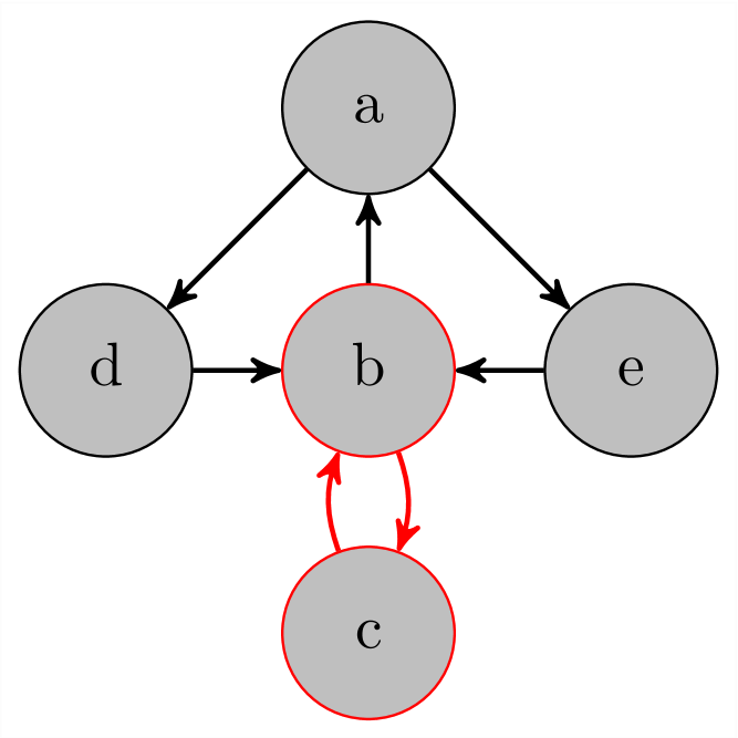
(a) Selection of a Cycle

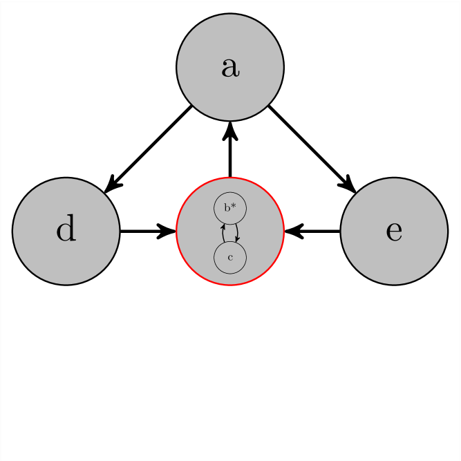
(b) After a Reduction Step

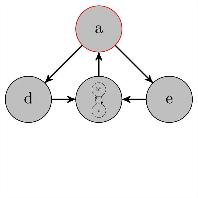
(c) Selection of a Mode to Split

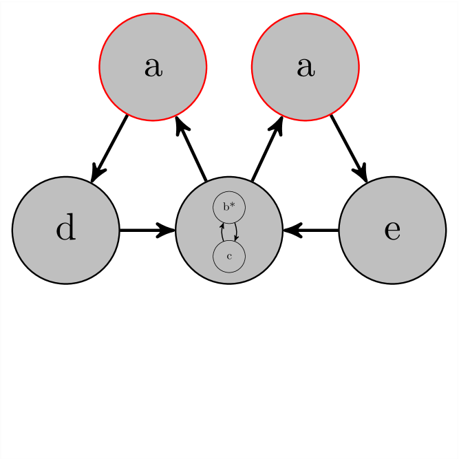
(d) After a Mode-splitting step

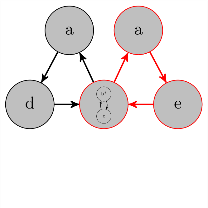
(e) Selection of a Cycle

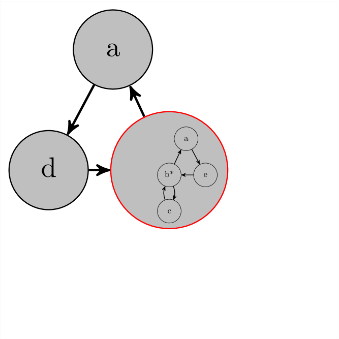
(f) After a Reduction Step

Figure 1: A Sketch of the Decomposition

The decomposition technique introduces a so-called constraint graph. In the constraint graph, vertices are labeled with mode constraints and transition constraints for self-loops, i. e., $m_{1}=m_{2}$ while edges are labeled with transition constraints for non-self-loops, i. e., $m_{1}\neq m_{2}$. Obviously, any solution to the constraint graph is a solution to Theorem  1. The graph structure is exploited in two ways:

1. The constraint graph is partitioned into finitely many strongly connected components (SCCs). A trajectory entering an SCC of the corresponding hybrid automaton may either converge to 0 within the SCC or leave the SCC in finite time. In any case, once entered, an SCC might not be entered again. This allows us to compute LLFs for each SCC separately.

2. Each SCC is further partitioned into (overlapping) cycles. LLFs for modes in a cycle can also be computed separately but compatibility – wrt. constraints on the edges – has to be assured somehow. Compatibility can be guaranteed if the cycles are examined successively in the following way: A cycle is selected and replaced by an underapproximation of the feasible set of its constraints, i. e., finitely many solutions (candidate LLFs) to the constraints of that cycle. Since the constraints describe a convex problem, conical combinations of the candidate LLFs satisfy the constraints, too. This step is called a reduction step. The reduction step collapses all vertices that lie only on that cycle and replaces references to LLFs in the constraints of adjacent edges by conical combinations of the candidate LLFs. This allows us to prove stability of each cycle separately while, cycle-by-cycle, ensuring compatibility of the feasible sets of the (overlapping) cycles.
   The reduction step is visualized in 1(a) and 1(b): In the former, a cycle is selected and in the latter, the cycle is replaced by a finite set of solutions of the corresponding optimization problem – visualized by collapsing the cycle into a single vertex.

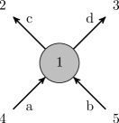
(a) Before splitting

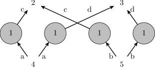
(b) After splitting

Figure 2: The Mode-Splitting Step

The reduction step is more efficient if the cycle is connected to the rest of the graph by at most one vertex. We call such a cycle an outer cycle and the vertex a border vertex. On one hand, if the graph contains an outer cycle, then the cycle can be collapsed into a single vertex which replaces the border vertex. Thus, the feasible set of the cycle’s constraints is replaced by a set of candidate LLFs. On the other hand, if the graph does not contain an outer cycle, then another step, called a mode-splitting step, is performed. In the mode-splitting step, a single vertex is replaced by a copy per pair of incoming and outgoing edges. This is visualized Figure  2. In 2(a), vertex 1 is connected to four other vertices by two incoming and two outgoing edges. In 2(b), vertex 1 is replaced by four copies, where each one is connected to exactly one incoming and one outgoing edge. Depending on the order in which vertices are chosen for mode-splitting, one can make a cycle connected to the rest of the graph by exactly one vertex and then perform a reduction step. Clearly, the order of mode-splitting and reduction steps does not only affect the termination of the procedure, but also the size of the graph and, therefore, the number of cycles that have to be reduced. With a good order of reduction and mode-splitting steps, one ends up with a single cycle for which the following holds: The successful computation of candidate LLFs implies the existence of a piecewise Lyapunov function for the whole SCC.

Continuing on the example given in Figure  1: In 1(c), there are no outer cycles, thus, a mode-splitting step is performed: the vertex a is selected, copied twice, and each path is routed through one copy. The result is shown in 1(d). Since the result contains outer cycles, we can select an outer cycle as in 1(e) and perform another reduction step resulting a single cycle being left. 1(f) shows the result.

Automatically Computing Lyapunov Functions

To compute Lyapunov functions needed for decomposition as well as for the monolithic approaches each Lyapunov function is instantiated by a template involving free parameters. Using this Lyapunov function templates a constraint system corresponding to Theorem  1 is generated. Such a constraint system is then relaxed by a series of relaxations involving 1. the so-called S-Procedure [3] which restricts the constraints to certain regions and 2. the sums-of-squares (SOS) decomposition [18] which allows us to rewrite the polynomials as linear matrix inequalities (LMI). These LMIs in turn can be solved by Semidefinite Programming (SDP) [3]. Instances of solvers are CSDP [2] and SDPA [5]. These solvers typically use some kind of interior point methods and numerically approximate a solution. While this is very fast, such numerical solvers sometimes suffer from numerical inaccuracies. Therefore, constraints may be strengthened by adding additional “gaps”. These gaps make the constraints more robust against numerical issues but sometimes result in the feasible set becoming empty.

These the gaps further limit the use of the decomposition as each reduction now “doubly” shrinks the feasible set: via gaps and via computing finitely many candidate LLFs.

4 Relaxation of the Graph Structure

In this section, we show how the decomposition can be improved by our graph structure-based relaxation. Consider the underlying digraph $\mathscr{G}=(\mathscr{V},\mathscr{E})$ of a hybrid automaton with the set of vertices $\mathscr{V}=\mathcal{M}$ and the set of edges $\mathscr{E}=\mathopen{}\mathclose{{}\left\{\mathopen{}\mathclose{{}\left(m_{1},m_{2}}\right)\;\middle|\;\exists\mathopen{}\mathclose{{}\left(m_{1},\mathit{G},\mathit{U},m_{2}}\right)\in\mathcal{T}}\right\}$. Note that the underlying graph has at most a single edge between any two vertices while the hybrid automaton might have multiple transitions between two modes. The density of the graph $\mathscr{G}$ is the fraction of the number of edges in the graph and the maximum possible number of edges in a graph of the same size, i. e., $\frac{|\mathscr{E}|}{|\mathscr{V}|(|\mathscr{V}|-1)}$.

The idea is to identify a set of modes of a hybrid automaton whose graph structure is dense. This can, for example, be done by a clique-finding or dense-subgraph-finding algorithm. A clique is a complete subgraph, i. e., having a density of $1$. Our relaxation then rewires the transitions such that the resulting automaton immediately exhibits a structure well-suited for decomposition. By “well-suited,” we mean that the graph structure contains mainly outer cycles.

The reason, that our relaxation technique plays so well with the decomposition technique, is as follows: if a hybrid system exhibits a dense graph structure, then the decomposition results in a huge blow-up. This blow-up is a result of the splitting step. The splitting step separates vertices shared between cycles, i. e., if there is more than one vertex shared between two or more cycles, then multiple copies are created. Thus, the higher the density of the graph structure is, the higher the blow-up gets. Further, if many cycles share many vertices – as in dense graphs – then whole cycles get copied and each copy requires solving an optimization problem and underapproximating the problem’s feasible set. In contrast, our relaxation overapproximates the discrete behavior by putting each vertex in its own cycle and connecting this vertex by a new “fake” vertex. This reduces the number of optimization problems to be solved and the number of feasible sets to be underapproximated.

In the following, we define the relaxation operator. Then we give an algorithm which applies the relaxation integrated with decomposition. Finally, we prove termination and implication of stability of the hybrid automaton which has been relaxed.

Definition 3.

The graph structure relaxed hybrid automaton $\mathit{Rlx}\mathopen{}\mathclose{{}\left(\mathcal{H},\mathcal{M}_{d}}\right)=(\mathcal{V}^{\sharp},\mathcal{M}^{\sharp},\mathcal{T}^{\sharp},\mathit{Flow}^{\sharp},\mathit{Inv}^{\sharp})=\mathcal{H}^{\sharp}$ of a hybrid automaton $\mathcal{H}=(\mathcal{V},\mathcal{M},\mathcal{T},\mathit{Flow},\mathit{Inv})$ wrt. the sub-component $\mathcal{M}_{d}\subseteq\mathcal{M}$ is defined as follows

$$\mathcal{V}^{\sharp}=\; \mathcal{V},$$

$$\mathcal{M}^{\sharp}=\; \mathcal{M}\mathbin{\mathaccent 0{\cdot}\cup}\{m_{c}\},$$

$$\mathcal{T}^{\sharp}=\; \mathopen{}\mathclose{{}\left\{\mathopen{}\mathclose{{}\left(m_{1},\mathit{G},\mathit{U},m_{2}}\right)\;\middle|\;\begin{matrix}\mathopen{}\mathclose{{}\left(m_{1},\mathit{G},\mathit{U},m_{2}}\right)\in\mathcal{T},\\ \{m_{1},m_{2}\}\cap\mathcal{M}_{d}=\emptyset\end{matrix}}\right\}$$

$$\bigcup\mathopen{}\mathclose{{}\left\{\begin{matrix}\mathopen{}\mathclose{{}\left(m_{1},\mathit{G},\mathrm{id},m_{c}}\right),\\ \mathopen{}\mathclose{{}\left(m_{c},\mathit{G},\mathit{U},m_{2}}\right)\end{matrix}\;\middle|\;\begin{matrix}\mathopen{}\mathclose{{}\left(m_{1},\mathit{G},\mathit{U},m_{2}}\right)\in\mathcal{T},\\ \{m_{1},m_{2}\}\cap\mathcal{M}_{d}\neq\emptyset\end{matrix}}\right\},$$

$$\mathit{Flow}^{\sharp}\mathopen{}\mathclose{{}\left(m}\right)=\; \begin{cases}\mathtt{zero}&\text{ if }m=m_{c}\\ \mathit{Flow}\mathopen{}\mathclose{{}\left(m}\right)&\text{ otherwise, }\end{cases}$$

$$\mathit{Inv}^{\sharp}\mathopen{}\mathclose{{}\left(m}\right)=\; \begin{cases}\emptyset&\text{ if }m=m_{c}\\ \mathit{Inv}\mathopen{}\mathclose{{}\left(m}\right)&\text{ otherwise, }\end{cases}$$

where $\mathtt{zero}:\mathcal{S}\to\mathcal{P}\mathopen{}\mathclose{{}\left(\mathcal{S}}\right)$ is a function assigning $\mathbf{0}$ to each $\mathbf{x}\in\mathcal{S}$, i. e., $\dot{\mathbf{x}}\in\{\mathbf{0}\}$.

In $\mathcal{T}^{\sharp}$ in Definition  3, we replace each transition $\mathopen{}\mathclose{{}\left(m_{1},\mathit{G},\mathit{U},m_{2}}\right)\in\mathcal{T}$ connected to at least one mode in $\mathcal{M}_{d}$ with two transitions: one connecting the old source mode $m_{1}$ with the new mode $m_{c}$ and the other connecting $m_{c}$ with the old target mode $m_{2}$. We call this step a transition-splitting step where the result is a pair of transitions which is called split transition and the set of all split transitions is denoted by $\mathit{ST}$.

Intuitively, the introduced mode $m_{c}$ is a dummy mode whose invariant always evaluates to false and the flow function does not change the valuations of the continuous variables. Indeed, the mode cannot be entered and thus, a trajectory taking an ingoing transition must, immediately, take an outgoing transition. The sole reason to add the mode is changing the structure of the hybrid system’s underlying graph: the new structure contains mainly cycles that are connected via $m_{c}$.

input : A hybrid automaton $\mathcal{H}$, a dense sub-component $\mathcal{M}_{d}$ of $\mathcal{H}$.

output : The relaxed version of $\mathcal{H}$, a set of split transitions $\mathit{ST}$, the central mode $m_{c}$.

1 $m_{c}\leftarrow$ newMode();

2 $\mathcal{H}.\mathcal{M}\leftarrow\mathcal{H}.\mathcal{M}\cup\{m_{c}\}$;

3 $\mathcal{H}.\mathit{Flow}\mathopen{}\mathclose{{}\left(m_{c}}\right)\leftarrow\mathtt{zero}$;

4 $\mathcal{H}.\mathit{Inv}\mathopen{}\mathclose{{}\left(m_{c}}\right)\leftarrow\emptyset$;

5 $\mathcal{T}\leftarrow\mathcal{H}.\mathcal{T}$;

6 foreach $t=\mathopen{}\mathclose{{}\left(m_{1},\mathit{G},\mathit{U},m_{2}}\right)\in\mathcal{T}$ do

7       if $\{m_{1},m_{2}\}\cap\mathcal{M}_{d}\neq\emptyset$ then

             // split the transitions into two parts

8             $t_{1}\leftarrow\mathopen{}\mathclose{{}\left(m_{1},\mathit{G},\mathrm{id},m_{c}}\right)$;

9             $t_{2}\leftarrow\mathopen{}\mathclose{{}\left(m_{c},\mathit{G},\mathit{U},m_{2}}\right)$;

             // replace the transition by the two parts

10             $\mathcal{H}.\mathcal{T}\leftarrow(\mathcal{H}.\mathcal{T}\setminus\{t\})\cup\{t_{1},t_{2}\}$;

             // keep account of split transitions

11             $\mathit{ST}\leftarrow\mathit{ST}\cup\{(t_{1},t_{2})\}$

12      

Algorithm 1 The Relaxation Function

input : A relaxed hybrid automaton $\mathcal{H}$, a set of split transitions $\mathit{ST}$, a pair of split transitions $\mathopen{}\mathclose{{}\left(t_{1},t_{2}}\right)$, where $t_{1}=\mathopen{}\mathclose{{}\left(m_{1},\mathit{G},\mathrm{id},m_{c}}\right)$, $t_{2}=\mathopen{}\mathclose{{}\left(m_{c},\mathit{G},\mathit{U},m_{2}}\right)$ and $m_{c}$ is the central mode.

output : A relaxed hybrid automaton $\mathcal{H}$ with one split transition being reconstructed, the set of split transitions $\mathit{ST}$

// reconstruct the original transition

1 $t\leftarrow\mathopen{}\mathclose{{}\left(m_{1},\mathit{G},\mathit{U},m_{2}}\right)$;

// replace the split transition $(t_{1},t_{2})$ by $t$

2 $\mathcal{H}.\mathcal{T}\leftarrow(\mathcal{H}.\mathcal{T}\setminus\{t_{1},t_{2}\})\cup\{t\}$;

// update the set of split transitions

3 $\mathit{ST}\leftarrow\mathit{ST}\setminus\{(t_{1},t_{2})\}$;

// remove $m_{c}$ iff unconnected

4 if $\mathit{ST}=\emptyset$ then

5       $\mathcal{H}.\mathcal{M}\leftarrow\mathcal{H}.\mathcal{M}\setminus\{m_{c}\}$;

6      

Algorithm 2 The Reconstruction Function

input : A hybrid automaton $\mathcal{H}$, a set of modes $\mathcal{M}_{d}$ corresponding to a dense subgraph.

output : stable if the $\mathcal{H}$ is stable and failed otherwise.

// relax the graph structure

1 $\mathcal{H},\mathit{ST},m_{c}\leftarrow$ relax($\mathcal{H},\mathcal{M}_{d}$);

2 while $\mathit{ST}\neq\emptyset$ do

       // apply decomposition

3       result $\leftarrow$ applyDecomposition($\mathcal{H}$);

4       if result is stable then

5             return stable;

6            

       // apply reconstruction

7       if $\exists(t_{1},t_{2})\in\mathit{ST}:\{t_{1},t_{2}\}\cap\textnormal{{failedSubgraph({{result}})}}\neq\emptyset$ then

8             $\mathcal{H},\mathit{ST}\leftarrow$ reconstruct($\mathcal{H},\mathit{ST},\mathopen{}\mathclose{{}\left(t_{1},t_{2}}\right),m_{c}$);

9            

10       else

11             return result;

12            

13      

// apply decomposition on the original automaton

14 result $\leftarrow$ applyDecomposition($\mathcal{H}$);

15 return result;

Algorithm 3 The Integrated Relaxation and Decomposition Algorithm

Next, we show how to integrate decomposition and relaxation. Pseudo-code of the relaxation function and a reconstruction function – which step-by-step reverts the relaxation – can be found in Algorithm  1 and Algorithm  2, respectively. Algorithm  3 gives pseudo-code of the main algorithm. The main algorithm works as follows: Step 1) The function relax relaxes the graph structure of the hybrid automaton $\mathcal{H}$ and generates the set of split transitions $\mathit{ST}$. Step 2) If the set $\mathit{ST}$ is empty, then call applyDecomposition with the original automaton and return the result – this function applies the original decompositition technique as described in Section  3. Step 3) Otherwise, apply applyDecomposition on the current relaxed form of the automaton. If the result is stable, then return the result. Otherwise, if the original decompositional technique has failed, then it returns a failed subgraph that is a subgraph for which it was unable to find Lyapunov functions. Step 4) Choose a split transition from the set $\mathit{ST}$ which also belongs to the failed subgraph. It is then used to reconstruct a transition from the original hybrid automaton. Then execution is continued with step 2. Step 5) If no such split transition exists, then the algorithm fails and returns the failed subgraph since this failing subgraph will persist in the automaton. Further reverting the relaxation cannot help because no split transition is contained in the failed subgraph.

Next, we prove termination and soundness of the algorithm. Here, soundness indicates that a Lyapunov function-based stability certificate for a relaxed automaton implies stability of the original, unmodified automaton. In particular, the local Lyapunov functions of the relaxed hybrid automaton are valid local Lyapunov functions for the original automaton.

Termination of the Integrated Algorithm

Theorem 2.

The proposed algorithm presented in Algorithm  3 terminates.

Proof.

The function relax terminates since the copy of the set of transitions of $\mathcal{H}$ is finite and is not modified in the course of the algorithm. The while-loop terminates if either an applyDecomposition is successful, no pair for reconstruction can be identified, or the set $\mathit{ST}$ is empty. In the first two cases, the algorithm terminates directly. For the last case, we assume that no call to applyDecomposition is successful and a spilt transition is always found. Then, in each iteration of the loop, one edge is removed from $\mathit{ST}$. The set $\mathit{ST}$ is finite because the relaxation function relax splits only finitely many edges. Thus, the set $\mathit{ST}$ becomes eventually empty. Therefore, the loop terminates. ∎

Preservation of Stability

Theorem 3.

For any hybrid automaton $\mathcal{H}$ and a sub-component $\mathcal{M}_{d}$, it holds: If a family of local Lyapunov functions $(V_{m})$ proving $\mathit{Rlx}\mathopen{}\mathclose{{}\left(\mathcal{H},\mathcal{M}_{d}}\right)$ to be GAS exists, then there exists a family of local Lyapunov functions for $\mathcal{H}$ proving $\mathcal{H}$ to be GAS.

Proof.

Given a hybrid automaton $\mathcal{H}=(\mathcal{V},\mathcal{M},\mathcal{T},\mathit{Flow},\mathit{Inv})$. Let $\mathit{Rlx}\mathopen{}\mathclose{{}\left(\mathcal{H},\mathcal{M}_{d}}\right)=(\mathcal{V}^{\sharp},\mathcal{M}^{\sharp},\mathcal{T}^{\sharp},\mathit{Flow}^{\sharp},\mathit{Inv}^{\sharp})\allowbreak=\mathcal{H}^{\sharp}$, be a graph structure-relaxed version of $\mathcal{H}$ where $\mathcal{M}_{d}\subseteq\mathcal{M}$ is the sub-component of $\mathcal{H}$ that has been relaxed. Further, let $(V_{m})$ be the family of local Lyapunov functions that prove stability of $\mathcal{H}^{\sharp}$ and let $\mathit{ST}$ be the set of split transitions – some transition may have been reconstructed. Now, it must be shown that $V_{m}$ are valid Lyapunov functions for $\mathcal{H}$.
The mode constraints of Theorem  1 trivially hold, since $\mathit{Rlx}$ alters neither the flow functions nor the invariants, i. e., $\forall m\in\mathcal{M}:\mathit{Flow}^{\sharp}\mathopen{}\mathclose{{}\left(m}\right)=\mathit{Flow}\mathopen{}\mathclose{{}\left(m}\right)\land\mathit{Inv}^{\sharp}\mathopen{}\mathclose{{}\left(m}\right)=\mathit{Inv}\mathopen{}\mathclose{{}\left(m}\right)$. The transition constraint also holds for all transitions that are not altered by $\mathit{Rlx}$ or have been reconstructed, i. e., $\mathcal{T}\cap\mathcal{T}^{\sharp}$. Now assume that $t\in\mathcal{T}\setminus\mathcal{T}^{\sharp}$ is an arbitrary transition for which the transition constraint does not hold. We show that this leads to a contradiction. Due to the definition of $\mathit{Rlx}$ all transition in $\mathcal{T}\setminus\mathcal{T}^{\sharp}$ are split transitions and there is a corresponding pair in $\mathit{ST}$. Let $\mathopen{}\mathclose{{}\left(t_{1},t_{2}}\right)\in\mathit{ST}$ be the pair corresponding to $t=(m_{1},\mathit{G},\mathit{U},m_{2})$. Since $(V_{m})$ is a valid family of local Lyapunov function for $\mathcal{H}^{\sharp}$, the transition constraint holds for all transitions in $\mathcal{T}^{\sharp}$. In particular, the transition constraint holds for $t_{1}=(m_{1},\mathit{G},\mathrm{id},m_{c})$ and $t_{2}=(m_{c},\mathit{G},\mathit{U},m_{2})$. Thus,

$$\forall x\in\mathit{G}:V_{m_{c}}\mathopen{}\mathclose{{}\left(\mathrm{id}\mathopen{}\mathclose{{}\left(x}\right)}\right)\leq V_{m_{1}}\mathopen{}\mathclose{{}\left(x}\right)\land\forall x\in\mathit{G}:V_{m_{2}}\mathopen{}\mathclose{{}\left(\mathit{U}\mathopen{}\mathclose{{}\left(x}\right)}\right)\leq V_{m_{c}}\mathopen{}\mathclose{{}\left(x}\right)\text{.}$$

It follows, that

$$\forall x\in\mathit{G}:V_{m_{2}}\mathopen{}\mathclose{{}\left(\mathit{U}\mathopen{}\mathclose{{}\left(x}\right)}\right)\leq V_{m_{c}}\mathopen{}\mathclose{{}\left(x}\right)\leq V_{m_{1}}\mathopen{}\mathclose{{}\left(x}\right)\text{.}$$

Therefore, the transition constraint holds for $t$. But this contradicts the assumption. $\lightning$ ∎

While Theorem  3 shows that stability of the relaxed automaton yields stability of the original automaton, the contrary is not true. Figure  3 shows a hybrid system where the relaxation renders the system unstable. This example exploits that the relaxation may introduce spurious trajectories. This happens if there are transitions with overlapping guard sets connected to the central mode $m_{c}$. A trajectory of the relaxed automaton might then take the first part of a split transition to the central mode $m_{c}$ and continues with the second part of a different split transition. A transition corresponding to this behavior might not exist in the unmodified hybrid automaton. While this does not render our approach being incorrect, it may lead to difficulties since these extra trajectories have to be GAS, too. In case of the system in Figure  3, new trajectories are introduced which allow a trajectory to jump back from the mode L to H by taking the transitions $t_{1},t_{2}$. This behavior corresponds to leaving L by the right self-loop and entering H by the left self-loop, which is obviously impossible. However, due to the update the value of $x$ might increase as $1+0.01(x-1)(x-10)>1$ for $x<1$.

In general our relaxation introduces conservatism which is again reduced step-by-step by the reconstruction. The degree of conservatism highly depends on the guards of the transitions since the central mode relates all LLFs of modes in $\mathcal{M}_{d}$. Therefore, if more guards are overlapping, more LLFs have to be compatible even if not needed in the original automaton.

One possibility to counter-act this issue is to introduce a new continuous variable in the relaxed automaton which is set to a unique value per split transition: the update function of the first part of a split transition sets the value used to guard the second part of the transition. Indeed, this trick discards any spurious trajectories for the price of an additional continuous variable. However, since the values of that variable are somewhat artificial, a Lyapunov function may not make use of that variable. Thus, this trick will not ease satisfying the conditions of the Lyapunov theorem in general.

(a) The unmodified (stable) version.

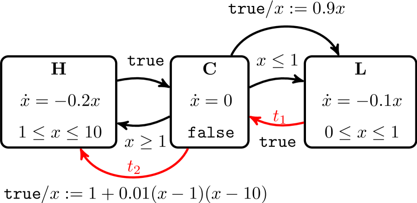
(b) The relaxed (unstable) version.

Figure 3: A Hybrid System; Unstable after Relaxation

5 Application of the Relaxation

In this section we present three examples where the graph structure-based relaxation suggested in this paper improves the application of the decomposition technique. The first example deals with the automatic cruise controller (ACC) of [9]. The second example is the fully connected digraph $K_{3}$. The $K_{3}$ does not represent a concrete hybrid automaton but a potential graph structure of a hybrid automaton. The last example is a spidercam. Here, the graph is not as fully connected as the $K_{3}$ example, but its density is already too high to apply decomposition directly.

We have implemented the decomposition and relaxation in python. Table  1 gives the graph properties and a comparison of the number of reduction steps required by the decomposition with and without relaxation (in the best case). The given data was obtained without actually computing Lyapunov functions focusing on the graph related part of the decomposition. In fact, computing Lyapunov functions for the spidercam via decomposition without our relaxation fails after 18 steps.

			Decomposition			With Relaxation
Graph Structure	Nodes ($n$)	Edges	Reductions	Mode-Splittings	Time	Reductions	Time
directed $K_{1}$	1	0	0	0	0.04s	0	0.04s
directed $K_{2}$	2	2	1	0	0.04s	2	0.04s
directed $K_{3}$	3	6	6	4	0.21s	3	0.05s
directed $K_{4}$	4	12	47	25	1.15s	4	0.05s
directed $K_{5}$	5	20	1852	352	13h22m	5	0.05s
Spidercam	9	32	753	287	1h46m	9	0.06s
Cruise Controller	6	11	7	6	0.060s	6	0.06s

Table 1: Comparison of the Decomposition with and without Relaxation

Example 1: The Automatic Cruise Controller (ACC)

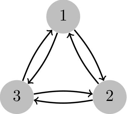
(a) original

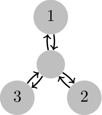
(b) relaxed

Figure 4: The $K_{3}$.

Figure 5: The Automatic Cruise Controller [9]

The automatic cruise controller (ACC) regulates the velocity of a vehicle. Figure  5 shows the controller as an automaton. The task of the controller is to approach a user-chosen velocity – indeed the variable $v$ represents the velocity relative to the desired velocity.

The ACC is globally asymptotically stable. It can be proven stable using the original decomposition technique (cf. [9, 8]). Indeed, the graph structure is sparse and thus, already well-suited for applying the decomposition technique directly. In fact, only one more cycle needs to be reduced compared to decomposition after relaxation (cf. Table  1). Even though the relaxation is not needed here, it also does not harm, though, it may be used for sparse graphs structures, too.

Example 2: The directed $K_{3}$

The directed $K_{n}$ is a fully connected digraph with $n$ nodes. The $K_{3}$ as well as a relaxed version of it is shown in Figure  5. In a fully connected digraph, there is a single edge from each node to each other node, resulting in a total number of $n(n-1)$ edges. The number of cycles, the decomposition technique has to reduce, grows very fast with $n$ which can be seen in Table  1. In comparison, the number of cycles in the relaxed version of the graph grows linearly with $n$, assuming that the edges can be concentrated. Otherwise, after the relaxation, each original node has $n-1$ incoming and $n-1$ outgoing edges where each edge connects the node with the central node $m_{c}$. Each such combination forms a cycle between $m_{c}$ and an original mode, giving a total of $n(n-1)(n-1)$ cycles in the worst case. This cubic growth is still much less than the number of reductions without relaxation.

Such a graph might not be the result of a by-hand designed system but might be the outcome of a synthesis or an automatic translation. However, the fast growth of the cycles also indicates the high number of reduction and therefore underapproximations.

Example 3: The Spidercam

A spidercam is a movable robot equipped with a camera. It is used at sport events such as a football matches. The robot is connected to four cables. Each cable is attached to a motor that is placed high above the playing field in a corner of a stadium. By winding and unwinding the cables – and thereby controlling the length of the cables, – the spidercam is able to reach nearly any position in the three-dimensional space above the playing field. Figure  6 shows a very simple model of such a spidercam in the plane. The target is to stabilize the camera at a certain position. The continuous variables $x$ and $y$ denote the distance relative to the desired position on the axis induced by the cables.

(a) unmodified

(b) relaxed

Figure 6: The Simple Planar Spidercam

In the model, we assume a high-level control of the motor engines, i. e., the movement is on axis $\dot{x}$ and $\dot{y}$ instead of a low-level control of each individual motor. The model has nine modes: one mode that controls the behavior while being close to the desired position, four modes corresponding to nearly straight movements along one of the axes and four modes cover the quadrants between the axes. The maximal velocity in the direction of each axis is limited from above by $0.6\frac{m}{s}$. Thus, in the four modes corresponding to the quadrants, the movement in each direction is at full speed. In the four modes corresponding to the axes, the movement on the particular axis is at full speed while the movement orthogonal to the axis is proportional to the distance. In the last mode, the speed in both directions is proportional to the distance.

The spidercam is globally asymptotically stable which can be proven fully automatically. However, it is not possible to obtain a piecewise Lyapunov function via decomposition without relaxation due to accumulating underapproximations of the partial solutions and the high number of cycles that have to be reduced. The reason is that each time a cycle is reduced, the feasible set of a subproblem is underapproximated by a finite set of solutions which finally results in a feasible set becoming empty and no LLFs can be found.

In contrast, relaxing the graph structure followed by applying the decomposition is successful immediately. In particular, no reconstruction step is required.

6 Summary

We have presented a relaxation technique based on the graph structure of a hybrid automaton. The relaxation exploits super-dense switching or cascaded transitions to modify the transitions of the hybrid automaton in a way that improves the decompositional proof technique of [11]. The idea is to re-route every transition through a new “fake” node. Thus, if in the original automaton a single transition is taken, then the relaxed automaton has to take the cascade of two transitions to achieve the same result. However, the relaxed automaton’s graph structure is better suited towards decomposition. Furthermore, the procedure can be automated which is very much desired as our focus is the automation of Lyapunov function-based stability proofs. Furthermore, in Section  5, we successfully employed the proposed technique in some examples.

The decompositional proof technique is particularly well-suited to prove stability of large-scale hybrid systems because it allows: 1. to decompose a monolithic proof into several smaller subproofs, 2. to reuse subproofs after modifying the hybrid system, and 3. to identify critical parts of the hybrid automaton. All these benefits are not available when the hybrid system exhibits a very dense graph structure of the automaton because that would lead to an enormous number of computational steps required in the decomposition. The proposed relaxation overcomes these matters in the best case. If the relaxation is too loose, then our technique falls back to step-by-step reconstruct the original automaton. Each step increases the effort needed for the decomposition until a proof succeeds or ultimately – in the worst case – the original automaton gets decomposed. Future research will include a tighter coupling of the decomposition and our relaxation approach. A first step will be to not discard the progress made by the decomposition but reuse the “gained knowledge”. Doing so will greatly reduce the computational effort.

References

- [1]
- [2] Brian Borchers (1999): CSDP, a C Library for Semidefinite Programming. Optim. Met. Softw. 10, pp. 613–623, 10.1080/10556789908805765.
- [3] Stephen Boyd & Lieven Vandenberghe (2004): Convex Optimization. Cambridge University Press, 10.1017/CBO9780511804441.
- [4] Parasara Sridhar Duggirala & Sayan Mitra (2012): Lyapunov abstractions for inevitability of hybrid systems. In: Proceedings of the 15th International Conference on Hybrid Systems: Computation and Control (HSCC’12), pp. 115–124, 10.1145/2185632.2185652.
- [5] Katsuki Fujisawa, Kazuhide Nakata, Makoto Yamashita & Mituhiro Fukuda (2007): SDPA Project : Solving Large-Scale Semidefinite Programs. JORSP 50(4), pp. 278–298. Available at http://ci.nii.ac.jp/naid/110006532053/en/.
- [6] J. Löfberg (2004): YALMIP : A Toolbox for Modeling and Optimization in MATLAB. In: Proceedings of the 13th Conference on Computer-Aided Control System Design (CACSD’04), Taipei, Taiwan, 10.1109/CACSD.2004.1393890.
- [7] M.A. Lyapunov (1907): Problème général de la stabilité du movement. In: Ann. Fac. Sci. Toulouse, 9, Université Paul Sabatier, pp. 203–474, 10.5802/afst.246. (Translation of a paper published in Comm. Soc. Math. Kharkow, 1893, reprinted Ann. Math. Studies No. 17, Princeton Univ. Press, 1949).
- [8] Eike Möhlmann & Oliver E. Theel (2013): Stabhyli: A Tool for Automatic Stability Verification of Non-Linear Hybrid Systems. In: Proceedings of the 16th International Conference on Hybrid Systems: Computation and Control (HSCC’13), pp. 107–112, 10.1145/2461328.2461347.
- [9] Jens Oehlerking (2011): Decomposition of Stability Proofs for Hybrid Systems. Ph.D. thesis, Carl von Ossietzky University of Oldenburg, Department of Computer Science, Oldenburg, Germany.
- [10] Jens Oehlerking, Henning Burchardt & Oliver E. Theel (2007): Fully Automated Stability Verification for Piecewise Affine Systems. In: Proceedings of the 10th international conference on Hybrid systems: computation and control (HSCC’07), pp. 741–745, 10.1007/978-3-540-71493-4_74.
- [11] Jens Oehlerking & Oliver E. Theel (2009): Decompositional Construction of Lyapunov Functions for Hybrid Systems. In: Proceedings of the 12th International Conference on Hybrid Systems: Computation and Control (HSCC’09), pp. 276–290, 10.1007/978-3-642-00602-9_20.
- [12] A. Papachristodoulou, J. Anderson, G. Valmorbida, S. Prajna, P. Seiler & P. A. Parrilo (2013): SOSTOOLS: Sum of squares optimization toolbox for MATLAB. Available at http://arxiv.org/abs/1310.4716.
- [13] Andreas Podelski & Silke Wagner (2007): Region Stability Proofs for Hybrid Systems. In: Formal Modelling and Analysis of Timed Systems (FORMATS’07), pp. 320–335, 10.1007/978-3-540-75454-1_23.
- [14] Pavithra Prabhakar (2012): Foundations for approximation based analysis of stability properties of hybrid systems. In: Proceedings of the 50th Annual Allerton Conference on Communication, Control, and Computing, pp. 1602–1609, 10.1109/Allerton.2012.6483412.
- [15] Pavithra Prabhakar, Geir E. Dullerud & Mahesh Viswanathan (2012): Pre-orders for reasoning about stability. In: Proceedings of the 15th International Conference on Hybrid Systems: Computation and Control (HSCC’12), pp. 197–206, 10.1145/2185632.2185662.
- [16] Pavithra Prabhakar, Jun Liu & Richard M. Murray (2013): Pre-orders for reasoning about stability properties with respect to input of hybrid systems. In: Proceedings of the International Conference on Embedded Software (EMSOFT’13), pp. 1–10, 10.1109/EMSOFT.2013.6658602.
- [17] Pavithra Prabhakar & Miriam Garcia Soto (2013): Abstraction Based Model-Checking of Stability of Hybrid Systems. In: Proceedings of the 25th International Conference on Computer Aided Verification (CAV’13), pp. 280–295, 10.1007/978-3-642-39799-8_20.
- [18] S. Prajna & A. Papachristodoulou (2003): Analysis of Switched and Hybrid Systems - Beyond Piecewise Quadratic Methods. In: American Control Conference, 2003. Proceedings of the 2003, 4, pp. 2779–2784 vol.4, 10.1109/ACC.2003.1243743.
- [19] Stefan Ratschan & Zhikun She (2010): Providing a Basin of Attraction to a Target Region of Polynomial Systems by Computation of Lyapunov-Like Functions. SIAM J. Control and Optimization 48(7), pp. 4377–4394, 10.1137/090749955.