Further consistency tests of the stability of fundamental couplings
Abstract
In a recent publication [Ferreira et al., Phys. Rev. D89 (2014) 083011] we tested the consistency of current astrophysical tests of the stability of the fine-structure constant and the proton-to-electron mass ratio (mostly obtained in the optical/ultraviolet) with combined measurements of , and the proton gyromagnetic ratio (mostly in the radio band). Given the significant observational progress made in the past year, we now revisit and update this analysis. We find that apparent inconsistencies, at about the two-sigma level, persist and are in some cases enhanced, especially for matter era measurements (corresponding to redshifts ). Although hidden systematics may be the more plausible explanation, we briefly highlight the importance of clarifying this issue, which is within the reach of state-of-the art observational facilities such as ALMA and ESPRESSO.
pacs:
04.50.Kd, 98.80.-kI Introduction
Tests of the stability of nature’s fundamental couplings are becoming an increasingly important probe of physics beyond the standard model Martins (2002); Uzan (2011). Very tight constraints stem from local laboratory tests using atomic clocks Rosenband et al. (2008), while astrophysical measurements allow a large lever arm which can probe the dynamics of the new degrees of freedom responsible for such putative variations, and potentially shed light on the dark energy enigma Amendola et al. (2012). There have been recent indications of possible variations Webb et al. (2011), which a dedicated Large Program at ESO’s Very Large Telescope is aiming to test Molaro et al. (2013); Rahmani et al. (2013); Evans et al. (2014).
Direct astrophysical measurements of the fine-structure constant and the proton-to-electron mass ratio are, in most cases, carried out the optical/ultraviolet (there are a few exceptions to this for the case), and up to redshifts now exceeding . On the other hand, in the radio band, and typically at lower redshifts, one can measure various combinations of , and the proton gyromagnetic ratio . In a recent work Ferreira et al. (2014) we carried out a joint statistical analysis of all existing data, in the context of a broad class of unification scenarios Coc et al. (2007), and highlighted some apparent inconsistencies which could be an indication that systematics may be affecting some of the data.
Given the significant observational progress made in the past fifteen months, both in measurements of Evans et al. (2014); Songaila and Cowie (2014) and in those of Albornoz Vásquez et al. (2014); Bagdonaite et al. (2015); Kanekar et al. (2015), in this work we will update our previous analysis. We start in Sect. II by briefly summarizing the theoretical assumptions underlying the class of unification scenarios we will assume, and then provide an up-to-date list of available measurements in Sect. III. Our consistency analysis is then presented in Sect. IV, and a brief outlook follows in Sect. V.
II Varying couplings and unification
The Standard Model (SM) of particle physics is one of the most respected buildings of modern physics. The desire to push it forward and understand its correctness at sufficiently high energy scales (the Planck mass, for instance) raises some open issues. One hint to the fact that the SM might be incomplete is the running of coupling constants with energy. These couplings are expected to meet at an energy scale of GeV. Considering this fact, it seems reasonable to think of a scenario in which all interactions stem from only one theory: a Grand Unified Theory (GUT).
In a general GUT, the symmetries of the SM—the gauge group —are unified into a larger symmetry group with only one coupling parameter at the GUT energy scale GeV. This coupling is assumed to be an independent parameter and it is allowed to vary. Assuming one such GUT, one can relate all couplings of SM interactions to only one, fundamental coupling. Since the latter can vary, all other related, lower energy, couplings must also vary and those variations should be related.
There are many models that attempt to unify the SM interactions. We will be working with a specific class of models that makes the following assumptions: the electroweak scale is derived by dimensional transmutation, all Yukawa couplings vary in the same way and the variation of the couplings is assumed to be a result of a dilaton-type scalar field. Under these assumptions it is possible to encapsulate the details of these class of theories in two parameters: and Campbell and Olive (1995); Coc et al. (2007). They are defined as proportionality factors between variations of fundamental couplings and they are highly model dependent:
| (1) |
| (2) |
where and , in which is the beta function coefficient for the SM gauge coupling () at an energy scale smaller than the unification scale, is the QCD mass scale, is the fine-structure constant, is the vacuum expectation value of the Higgs and stands for any of the Yukawa couplings (we’re assuming that all of them vary in the same way).
Using these two parameters, one can express, in a compact way, the varying-coupling character of a wide class of theories and, by constraining them, it is possible to shed some light on the specificities of a putative GUT. Hence, in what follows, we’ll use them to relate the variations of interest as Coc et al. (2007); Luo et al. (2011); Ferreira et al. (2012)
| (3) |
| (4) |
| (5) |
Note that in this class of models the proton gyromagnetic ratio is less sensitive to the parameters and than the proton-to-electron mass ratio. We will use this observation in some of our subsequent analysis. We also point out that in this class of models the behavior of the temperature-redshift relation provides a further consistency test, as first discussed in Avgoustidis et al. (2012, 2014).
III Current spectroscopic measurements
We now list the astrophysical measurements that will be used in our analysis. Unless otherwise stated, we will list them in units of parts per million (ppm). This is not meant to be an exhaustive list of all measurements. We typically use only the tightest available measurement for each astrophysical source. A few older measurements along other lines of sight have not been used, on the grounds that they would have no statistical weight in the analysis. Nevertheless, we will include some low-sensitivity but high-redshift measurements, as these are illustrative of the redshift range that may be probed by future facilities. As in Ferreira et al. (2014), whose list we update here, our two exceptions regarding measurements of the same source are
-
•
Measurements using different, independent techniques—typically this occurs with measurements of or combined measurements using different molecules, and
-
•
Measurements obtained with different spectrographs .
In these cases we do list the various available measurements.
| Object | z | Ref. | ||
| PKS1413135 | 0.247 | Kanekar et al. (2010) | ||
| PKS1413135 | 0.247 | Darling (2004) | ||
| PKS1413135 | 0.247 | Murphy et al. (2001) | ||
| B0218357 | 0.685 | Murphy et al. (2001) | ||
| J01340931 | 0.765 | Kanekar et al. (2012) | ||
| J23581020 | 1.173 | Rahmani et al. (2012) | ||
| J16230718 | 1.336 | Rahmani et al. (2012) | ||
| J23400053 | 1.361 | Rahmani et al. (2012) | ||
| J05010159 | 1.561 | Rahmani et al. (2012) | ||
| J10244709 | 2.285 | Curran et al. (2011) | ||
| J21350102 | 2.326 | Curran et al. (2011) | ||
| J16366612 | 2.517 | Curran et al. (2011) | ||
| H1413117 | 2.558 | Curran et al. (2011) | ||
| J14010252 | 2.565 | Curran et al. (2011) | ||
| J09110551 | 2.796 | Weiss et al. (2012) | ||
| J13373152 | 3.174 | Srianand et al. (2010) | ||
| APM08285255 | 3.913 | Curran et al. (2011) | ||
| MM18425938 | 3.930 | Curran et al. (2011) | ||
| PSS23221944 | 4.112 | Curran et al. (2011) | ||
| BR12020725 | 4.695 | Lentati et al. (2013) | ||
| J09185142 | 5.245 | Levshakov et al. (2012) | ||
| J11485251 | 6.420 | Lentati et al. (2013) |
Table 1 contains current joint measurements of several couplings. Compared to our earlier work we have added the measurements of Curran et al. (2011), which although not particularly sensitive complement the other measurements in terms of redshift coverage. (We thank Hugo Messias for bringing this reference to our attention.) Note that for the radio source PKS1413135 the three available measurements are sufficient to yield individual constraints on the variations of the three quantities at redshift . This analysis was done in Ferreira et al. (2013), yielding a null result at the two sigma confidence level.
| Object | z | (ppm) | Spectrograph | Ref. |
|---|---|---|---|---|
| 3 sources | 1.08 | HIRES | Songaila and Cowie (2014) | |
| HS15491919 | 1.14 | UVES/HIRES/HDS | Evans et al. (2014) | |
| HE05154414 | 1.15 | UVES | Molaro et al. (2008) | |
| HE05154414 | 1.15 | HARPS/UVES | Chand et al. (2006) | |
| HS15491919 | 1.34 | UVES/HIRES/HDS | Evans et al. (2014) | |
| HE00012340 | 1.58 | UVES | Agafonova et al. (2011) | |
| HE11041805A | 1.66 | HIRES | Songaila and Cowie (2014) | |
| HE22172818 | 1.69 | UVES | Molaro et al. (2013) | |
| HS19467658 | 1.74 | HIRES | Songaila and Cowie (2014) | |
| HS15491919 | 1.80 | UVES/HIRES/HDS | Evans et al. (2014) | |
| Q1101264 | 1.84 | UVES | Molaro et al. (2008) |
Table 2 contains individual measurements. Conservatively we only list measurements where data was acquired specifically for this purpose—but these are by now, in most cases, the ones with the smallest uncertainties. Compared to our previous analysis we have added the most recent Large Program result Evans et al. (2014) as well as the measurements of Songaila and Cowie (2014). We note that the weighted mean of the measurements on the table is
| (6) |
and thus, for the first time, the one-sigma statistical uncertainty is below ppm (although the key issue is that of possible systematics).
| Object | z | Method | Ref. | |
| B0218357 | 0.685 | // | Murphy et al. (2008) | |
| B0218357 | 0.685 | // | Kanekar (2011) | |
| PKS1830211 | 0.886 | / | Henkel et al. (2009) | |
| PKS1830211 | 0.886 | Ilyushin et al. (2012) | ||
| PKS1830211 | 0.886 | Muller et al. (2011) | ||
| PKS1830211 | 0.886 | Bagdonaite et al. (2013) | ||
| J2123005 | 2.059 | / (VLT) | van Weerdenburg et al. (2011) | |
| J2123005 | 2.059 | / (Keck) | Malec et al. (2010) | |
| HE00271836 | 2.402 | Rahmani et al. (2013) | ||
| Q2348011 | 2.426 | Bagdonaite et al. (2012) | ||
| Q0405443 | 2.597 | King et al. (2008) | ||
| J0643504 | 2.659 | Albornoz Vásquez et al. (2014) | ||
| Q0528250 | 2.811 | / | King et al. (2011) | |
| Q0347383 | 3.025 | Wendt and Reimers (2008) | ||
| J14432724 | 4.224 | Bagdonaite et al. (2015) |
Table 3 contains individual measurements. Note that several different molecules can be used, and in the case of the gravitational lens PKS1830211 several independent measurements exist. Currently ammonia is the most common at low redshift, though others such as methanol, peroxide, hydronium and methanetiol have a greater potential in the context of facilities like ALMA Kozlov and Levshakov (2013). At higher redshifts molecular hydrogen is the most common.
The tightest available constraint was obtained in PKS1830211, from observations of methanol transitions Bagdonaite et al. (2013). A recent analysis leads to a nominally tighter bound Kanekar et al. (2015), but the authors suggest caution in using that result due to possible systematics; conservatively, we have therefore kept the earlier measurement. As for measurements along the line of sight towards J0643504, we have similarly listed the more conservative one, from Albornoz Vásquez et al. (2014) on the table; for comparison Bagdonaite et al. (2014) finds ppm.
The main update to these measurements is therefore the arrival of the first direct constraint on beyond Bagdonaite et al. (2015). Calculating the weighted mean of the low and high-redshift samples ( and , respectively, we find
| (7) |
| (8) |
in both cases this is a very mild evidence for a variation, though with different signs at high and low redshifts,
IV Consistency analysis
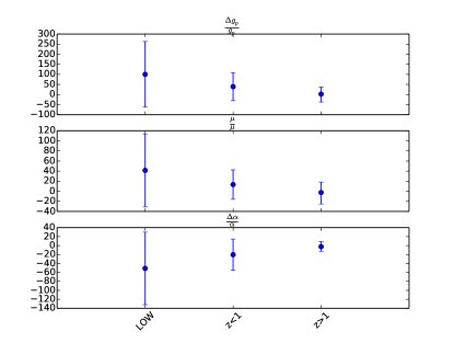
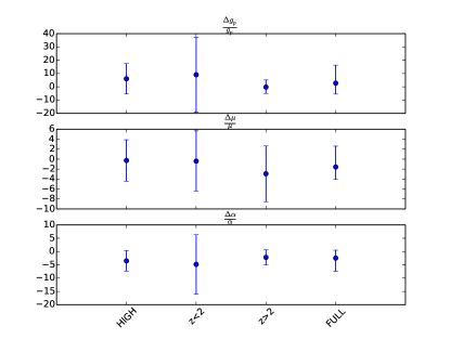
Note that the vertical scale is different in both sets of panels.
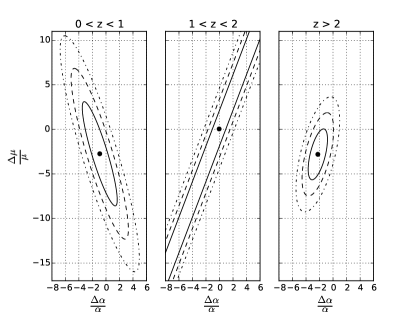
We start by determining the individual values of the three couplings that provide the best fit to the data in Table 1. The results are summarized in Fig. 1. We obtained the following one-sigma constraints for the full table
| (9) |
| (10) |
| (11) |
thus consistent with no variations. In addition to the full sample the figure also shows the results of the analysis for a few subsamples
-
•
(denoted Low in the plot, and containing only the measurements along the line-of-sight to PKS1413135 discussed in Ferreira et al. (2013)) versus (denoted High in the plot)
-
•
versus
-
•
versus
We note that the likelihood profiles are usually non-Gaussian, both here and in the analyses in the rest of this section. This explains why some of the confidence intervals are asymmetric.
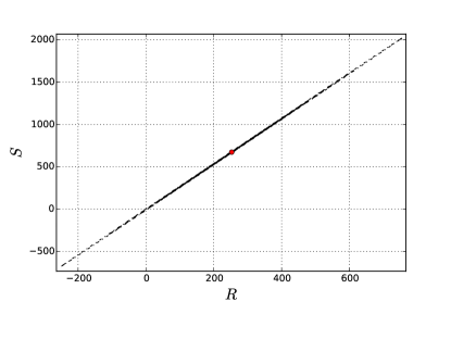
Fig. 2 shows the two-dimensional confidence levels in the plane of the unification parameters R and S discussed in Sect. II. The one dimensional marginalized likelihoods for each of them are
| (12) |
These are fully consistent with the naive expectations suggesting typical values around and Coc et al. (2007) as well as with the results of our earlier work Ferreira et al. (2014).
| Sample | ||
|---|---|---|
| Unconstrained | Unconstrained | |
| Full |
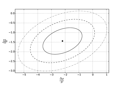
Since in this class of models the variations of are, for typical values of the parameters and , smaller than those of , it’s interesting to repeat some of the above analysis on the assumption that does not vary. These results are shown in Fig. 3, and the 1D marginalized constraints for the full sample and various subsamples are shown in Table 4.
Note that in this case there are again deviations (at up to the two sigma level) from the null result, which wasn’t the case in the full analysis where was also allowed to vary. This change stems from the reduction in uncertainties afforded by the assumption of a fixed (the shift in best-fit values is comparatively small), and is therefore not statistically significant. In the redshift range the individual values of both parameters are unconstrained by this dataset: only the combination is constrained, but this constraint does play a role in the full likelihood for this case. Finally, it’s also interesting to note that the degeneracy directions are different at high and low redshifts.
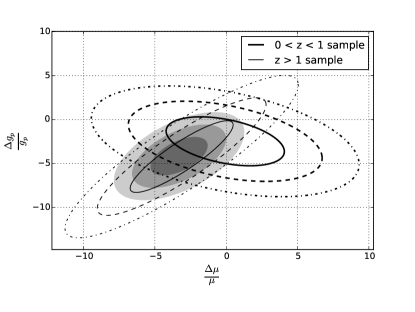
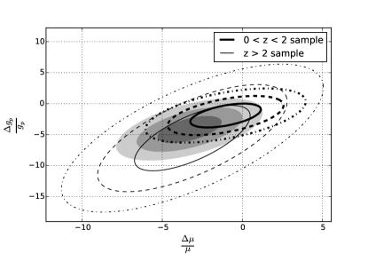
We can also reanalyze the data of Table 1 using the weighed mean value of Table 2 for (ie, Eq.6) as a prior. The results of this analysis are summarized in Fig. 4 and Table 5, both for the full sample and for high/low redshift subsamples. There is a mild (two-sigma) preference for negative variations of both quantities, which mostly stems from the higher redshift data. As before, note that the degeneracy directions change with redshift; this partly explains why the preference for negative variations is much stronger for the full sample than the subsamples. On the other hand, it could also be an indication that assuming a constant value for the parameters in this entire redshift range may be too simplistic.
| Sample | ||
|---|---|---|
| Full |
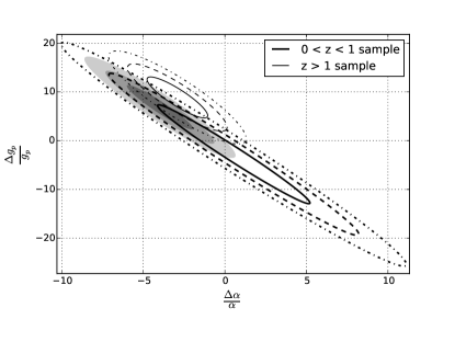
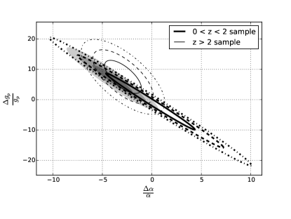
The complementary exercise can also be done: we can analyze the data of Table 1 using the weighed mean values of Table 3 for at low and high redshifts (ie, Eqs.7-8) as priors. The corresponding results are summarized in Fig. 5 and Table 6. We again considered both the full sample and high and low redshift subsamples. There is again a mild (two-sigma) preference for variations of both quantities, which again mostly stems from the higher redshift data. In this case the results are not as clear which is at least in part the result of a stronger degeneracy than in the previous case. One effect of the priors (with their slight preference for negative variations) is to lead to a preference for positive values of (while a negative value is preferred for ).
| Sample | ||
|---|---|---|
| Full |
As an additional check, if we assume that does not vary and use the weighed mean of Table 2 for as a prior for Table 1 we now find, at the two-sigma confidence level,
| (13) |
compared to the more general analysis summarized in Table 5 the central value is in good agreement, while the uncertainty is naturally reduced. Conversely, if we assume that is fixed and use the weighted mean value of Table 3 for we find, still at the two-sigma level
| (14) |
again, this is consistent with the results of Table 6, though with a significantly reduced uncertainty. Finally if we simultaneously use the weighted mean averages of Tables 2 and 3 as priors for and and use Table 1 to infer , we obtain at the two-sigma confidence level
| (15) |
V Conclusions
In this work we have fully updated an earlier analysis Ferreira et al. (2014) of the consistency of the various currently available astrophysical tests of the stability of fundamental couplings. Various combinations of , and can be measured in the radio band, while and can also be individually measured, mostly through observations in the optical/ultraviolet region. Taken together, they span very broad redshift range—approximately from to —although the sensitivity of current measurements is also quite heterogeneous: from about 0.1 ppm to more than 100 ppm.
Our results show that a joint analysis of all the combined measurements is consistent with no variations. However, joint analyses of the radio and optical/UV data tend to lead to mild evidence (specifically, at two-sigma confidence level) for variations at the few ppm level. This is especially the case at redshifts , corresponding to measurements in the matter era.
It is noteworthy that the sensitivity with which each parameter can be constrained is redshift dependent. The best direct individual constraints on (at the few ppm level) are currently in the redshift range , while those for are either at (from molecular Hydrogen measurements) or at (from measurements using other molecules, such as ammonia or methanol). Similarly, different products of , and can be constrained at different redshift. This is relevant for optimizing observational strategies and selecting targets for future facilities.
Admittedly the evidence for possible variations thus inferred is not strong, and the most likely explanation for them is that systematic errors have not been fully accounted for. In the case of the optical measurements, possible sources for these have recently been studied in some detail Molaro et al. (2013); Rahmani et al. (2013); Evans et al. (2014); Whitmore and Murphy (2015). In any case, clarifying these discrepancies is essential. Finding lines of sight where these measurements can be carried out both in the optical and in the radio bands would provide an ideal test of possible systematics, but the number of such targets is likely to be small.
A more immediate goal will be to extend the range of redshifts where sensitive measurements of and can be made. The imminent arrival of observational facilities such as ALMA and ESPRESSO will make this possible. This will signal the start of a new era of precision consistency tests of the current cosmological paradigm, which will continue with the E-ELT. A roadmap for these tests can be found in Martins (2015).
Acknowledgements.
This work was done in the context of the project PTDC/FIS/111725/2009 from FCT (Portugal). C.J.M. is also supported by an FCT Research Professorship, contract reference IF/00064/2012, funded by FCT/MCTES (Portugal) and POPH/FSE (EC).References
- Martins (2002) C. J. A. P. Martins, Phil.Trans.Roy.Soc.Lond. A360, 2681 (2002), arXiv:astro-ph/0205504 [astro-ph] .
- Uzan (2011) J.-P. Uzan, Living Rev.Rel. 14, 2 (2011), arXiv:1009.5514 [astro-ph.CO] .
- Rosenband et al. (2008) T. Rosenband, D. B. Hume, P. O. Schmidt, C. W. Chou, A. Brusch, L. Lorini, W. H. Oskay, R. E. Drullinger, T. M. Fortier, J. E. Stalnaker, S. A. Diddams, W. C. Swann, N. R. Newbury, W. M. Itano, D. J. Wineland, and J. C. Bergquist, Science 319, 1808 (2008).
- Amendola et al. (2012) L. Amendola, A. C. O. Leite, C. J. A. P. Martins, N. J. Nunes, P. O. J. Pedrosa, and A. Seganti, Phys.Rev. D86, 063515 (2012), arXiv:1109.6793 [astro-ph.CO] .
- Webb et al. (2011) J. K. Webb, J. A. King, M. T. Murphy, V. V. Flambaum, R. F. Carswell, et al., Phys.Rev.Lett. 107, 191101 (2011), arXiv:1008.3907 [astro-ph.CO] .
- Molaro et al. (2013) P. Molaro, M. Centurion, J. Whitmore, T. Evans, M. Murphy, et al., A. & A. 555, A68 (2013), arXiv:1305.1884 [astro-ph.CO] .
- Rahmani et al. (2013) H. Rahmani, M. Wendt, R. Srianand, P. Noterdaeme, P. Petitjean, P. Molaro, J. B. Whitmore, M. T. Murphy, M. Centurion, H. Fathivavsari, S. D’Odorico, T. M. Evans, S. A. Levshakov, S. Lopez, C. J. A. P. Martins, D. Reimers, and G. Vladilo, MNRAS 435, 861 (2013), arXiv:1307.5864 [astro-ph.CO] .
- Evans et al. (2014) T. M. Evans, M. T. Murphy, J. B. Whitmore, T. Misawa, M. Centurion, S. D’Odorico, S. Lopez, C. J. A. P. Martins, P. Molaro, P. Petitjean, H. Rahmani, R. Srianand, and M. Wendt, M.N.R.A.S. 445, 128 (2014).
- Ferreira et al. (2014) M. C. Ferreira, O. Frigola, C. J. A. P. Martins, A. M. R. V. L. Monteiro, and J. Solà, Phys.Rev. D89, 083011 (2014), arXiv:1405.0299 [astro-ph.CO] .
- Coc et al. (2007) A. Coc, N. J. Nunes, K. A. Olive, J.-P. Uzan, and E. Vangioni, Phys.Rev. D76, 023511 (2007), arXiv:astro-ph/0610733 [astro-ph] .
- Songaila and Cowie (2014) A. Songaila and L. Cowie, Astrophys.J. 793, 103 (2014), arXiv:1406.3628 [astro-ph.CO] .
- Albornoz Vásquez et al. (2014) D. Albornoz Vásquez, H. Rahmani, P. Noterdaeme, P. Petitjean, R. Srianand, and C. Ledoux, A. & A. 562, A88 (2014).
- Bagdonaite et al. (2015) J. Bagdonaite, W. Ubachs, M. Murphy, and J. Whitmore, Phys.Rev.Lett. 114, 071301 (2015), arXiv:1501.05533 [astro-ph.CO] .
- Kanekar et al. (2015) N. Kanekar, W. Ubachs, K. Menten, J. Bagdonaite, A. Brunthaler, et al., Mon.Not.Roy.Astron.Soc. 448, L104 (2015), arXiv:1412.7757 [astro-ph.CO] .
- Campbell and Olive (1995) B. A. Campbell and K. A. Olive, Phys.Lett. B345, 429 (1995), arXiv:hep-ph/9411272 [hep-ph] .
- Luo et al. (2011) F. Luo, K. A. Olive, and J.-P. Uzan, Phys.Rev. D84, 096004 (2011), arXiv:1107.4154 [hep-ph] .
- Ferreira et al. (2012) M. C. Ferreira, M. D. Julião, C. J. A. P. Martins, and A. M. R. V. L. Monteiro, Phys.Rev. D86, 125025 (2012), arXiv:1212.4164 [hep-ph] .
- Avgoustidis et al. (2012) A. Avgoustidis, G. Luzzi, C. J. A. P. Martins, and A. M. R. V. L. Monteiro, JCAP 1202, 013 (2012), arXiv:1112.1862 [astro-ph.CO] .
- Avgoustidis et al. (2014) A. Avgoustidis, C. J. A. P. Martins, A. M. R. V. L. Monteiro, P. E. Vielzeuf, and G. Luzzi, JCAP 1406, 062 (2014), arXiv:1305.7031 [astro-ph.CO] .
- Kanekar et al. (2010) N. Kanekar, J. N. Chengalur, and T. Ghosh, Ap.J.Lett. 716, L23 (2010), arXiv:1004.5383 [astro-ph.CO] .
- Darling (2004) J. Darling, Astrophys.J. 612, 58 (2004), arXiv:astro-ph/0405240 [astro-ph] .
- Murphy et al. (2001) M. Murphy, J. Webb, V. Flambaum, M. Drinkwater, F. Combes, et al., Mon.Not.Roy.Astron.Soc. 327, 1244 (2001), arXiv:astro-ph/0101519 [astro-ph] .
- Kanekar et al. (2012) N. Kanekar, G. I. Langston, J. T. Stocke, C. L. Carilli, and K. M. Menten, Ap.J.Lett. 746, L16 (2012), arXiv:1201.3372 [astro-ph.CO] .
- Rahmani et al. (2012) H. Rahmani, R. Srianand, N. Gupta, P. Petitjean, P. Noterdaeme, and D. A. Vásquez, MNRAS 425, 556 (2012), arXiv:1206.2653 [astro-ph.CO] .
- Curran et al. (2011) S. Curran, A. Tanna, F. Koch, J. Berengut, J. Webb, et al., Astron.Astrophys. 533, A55 (2011), arXiv:1108.0976 [astro-ph.CO] .
- Weiss et al. (2012) A. Weiss, F. Walter, D. Downes, C. Carrili, C. Henkel, et al., Astrophys.J. 753, 102 (2012), arXiv:1204.5614 [astro-ph.CO] .
- Srianand et al. (2010) R. Srianand, N. Gupta, P. Petitjean, P. Noterdaeme, and C. Ledoux, MNRAS 405, 1888 (2010), arXiv:1002.4620 [astro-ph.CO] .
- Lentati et al. (2013) L. Lentati, C. Carilli, P. Alexander, R. Maiolino, R. Wang, P. Cox, D. Downes, R. McMahon, K. M. Menten, R. Neri, D. Riechers, J. Wagg, F. Walter, and A. Wolfe, MNRAS , 721 (2013), arXiv:1211.3316 [astro-ph.CO] .
- Levshakov et al. (2012) S. A. Levshakov, F. Combes, F. Boone, I. I. Agafonova, D. Reimers, and M. G. Kozlov, A. & A. 540, L9 (2012), arXiv:1203.3649 [astro-ph.CO] .
- Ferreira et al. (2013) M. C. Ferreira, M. D. Julião, C. J. A. P. Martins, and A. M. R. V. L. Monteiro, Phys.Lett. B724, 1 (2013), arXiv:1305.7515 [astro-ph.CO] .
- Molaro et al. (2008) P. Molaro, D. Reimers, I. I. Agafonova, and S. A. Levshakov, European Physical Journal Special Topics 163, 173 (2008), arXiv:0712.4380 .
- Chand et al. (2006) H. Chand, R. Srianand, P. Petitjean, B. Aracil, R. Quast, and D. Reimers, A. & A. 451, 45 (2006), arXiv:astro-ph/0601194 .
- Agafonova et al. (2011) I. I. Agafonova, P. Molaro, S. A. Levshakov, and J. L. Hou, A. & A. 529, A28 (2011), arXiv:1102.2967 [astro-ph.CO] .
- Murphy et al. (2008) M. T. Murphy, V. V. Flambaum, S. Muller, and C. Henkel, Science 320, 1611 (2008), arXiv:0806.3081 [astro-ph] .
- Kanekar (2011) N. Kanekar, Astrophys.J. 728, L12 (2011), arXiv:1101.4029 [astro-ph.CO] .
- Henkel et al. (2009) C. Henkel, K. M. Menten, M. T. Murphy, N. Jethava, V. V. Flambaum, J. A. Braatz, S. Muller, J. Ott, and R. Q. Mao, A. & A. 500, 725 (2009), arXiv:0904.3081 [astro-ph.CO] .
- Ilyushin et al. (2012) V. V. Ilyushin, P. Jansen, M. G. Kozlov, S. A. Levshakov, I. Kleiner, W. Ubachs, and H. L. Bethlem, Phys.Rev. A85, 032505 (2012), arXiv:1201.2090 [chem-ph] .
- Muller et al. (2011) S. Muller, A. Beelen, M. Guélin, S. Aalto, J. H. Black, F. Combes, S. J. Curran, P. Theule, and S. N. Longmore, A. & A. 535, A103 (2011), arXiv:1104.3361 [astro-ph.CO] .
- Bagdonaite et al. (2013) J. Bagdonaite, M. Daprà, P. Jansen, H. L. Bethlem, W. Ubachs, et al., Phys.Rev.Lett. 111, 231101 (2013), arXiv:1311.3438 [astro-ph.CO] .
- van Weerdenburg et al. (2011) F. van Weerdenburg, M. Murphy, A. Malec, L. Kaper, and W. Ubachs, Phys.Rev.Lett. 106, 180802 (2011), arXiv:1104.2969 [astro-ph.CO] .
- Malec et al. (2010) A. L. Malec, R. Buning, M. T. Murphy, N. Milutinovic, S. L. Ellison, J. X. Prochaska, L. Kaper, J. Tumlinson, R. F. Carswell, and W. Ubachs, MNRAS 403, 1541 (2010), arXiv:1001.4078 [astro-ph.CO] .
- Bagdonaite et al. (2012) J. Bagdonaite, M. T. Murphy, L. Kaper, and W. Ubachs, MNRAS 421, 419 (2012), arXiv:1112.0428 [astro-ph.CO] .
- King et al. (2008) J. A. King, J. K. Webb, M. T. Murphy, and R. F. Carswell, Phys. Rev. Lett. 101, 251304 (2008), arXiv:0807.4366 [astro-ph] .
- King et al. (2011) J. A. King, M. T. Murphy, W. Ubachs, and J. K. Webb, MNRAS 417, 3010 (2011), arXiv:1106.5786 [astro-ph.CO] .
- Wendt and Reimers (2008) M. Wendt and D. Reimers, Eur.Phys.J.ST 163, 197 (2008), arXiv:0802.1160 [astro-ph] .
- Kozlov and Levshakov (2013) M. Kozlov and S. Levshakov, Annalen Phys. 525, 452 (2013), arXiv:1304.4510 [physics.atom-ph] .
- Bagdonaite et al. (2014) J. Bagdonaite, W. Ubachs, M. T. Murphy, and J. B. Whitmore, Astrophys.J. 782, 10 (2014), arXiv:1308.1330 [astro-ph.CO] .
- Whitmore and Murphy (2015) J. B. Whitmore and M. T. Murphy, Mon.Not.Roy.Astron.Soc. 447, 446 (2015), arXiv:1409.4467 [astro-ph.IM] .
- Martins (2015) C. J. A. P. Martins, Gen.Rel.Grav. 47, 1843 (2015), arXiv:1412.0108 [astro-ph.CO] .